Statistical fluctuations of correlators
in the Color Glass Condensate

Abstract

In the McLerran-Venugopalan model, correlators of Wilson lines are given by an average over a Gaussian ensemble of random color sources. In numerical implementations, these averages are approximated by a Monte-Carlo sampling. In this paper, we study the statistical error made with such a sampling, with emphasis on the momentum dependence of this error. Using the example of the dipole amplitude, we consider various approximants that are all equivalent in the limit of infinite statistics but differ with finite statistics and compare their statistical errors. For correlation functions that are translation invariant, we show that averaging over the barycenter coordinate drastically reduces the statistical error and more importantly modifies its momentum dependence.

• Institut de Physique Théorique, Université Paris-Saclay
  CEA, CNRS, F-91191 Gif-sur-Yvette, France

• European Centre for Theoretical Studies in Nuclear Physics
  and Related Areas (ECT*) and Fondazione Bruno Kessler
  Strada delle Tabarelle 286, I-38123 Villazzano, Italy

1 Introduction

In the Color Glass Condensate (CGC) effective theory [1, 2, 3, 4], the degrees of freedom internal to a high energy hadron or nucleus are split into two categories depending on their longitudinal momentum in the observer’s frame. The dynamical evolution of the fast modes is slowed down by time dilation, and therefore they are approximated as static constituents that carry a color current. The slow modes cannot be approximated in this way. Instead, they are treated as usual gauge fields, eikonally coupled to the color current produced by the fast modes. In this approximation, the evaluation of scattering amplitudes involving one or more high energy hadrons in the initial state can be formulated in terms of a Yang-Mills theory coupled to an external color current. However, it is important to realize that this current has event-by-event fluctuations. Indeed, this current reflects the precise configuration of the fast partons of the projectile at the time of the collision, which of course differs from one event to the next one.

A simple and popular model for the fluctuations of this color current is the McLerran-Venugopalan (MV) model [5, 6], which states that for a large enough projectile the fluctuations are Gaussian (one may view this as a consequence of the central limit theorem). More precisely, in the MV model, the color current of a high energy projectile moving in the $+z$ direction is parameterized as follows,

$$J^{\mu}_{a}(x)=\delta^{\mu+}\rho_{a}(x^{-},{\bm{x}}_{\perp}),$$

$$\big{<}\rho_{a}(x^{-},{\bm{x}}_{\perp})\big{>}=0,$$

$$\big{<}\rho_{a}(x^{-},{\bm{x}}_{\perp})\rho_{b}(y^{-},{\bm{y}}_{\perp})\big{>}=\mu^{2}(x^{-})\,\delta_{ab}\delta(x^{-}-y^{-})\delta({\bm{x}}_{\perp}-{\bm{y}}_{\perp})\;.$$ (1)

where $\rho_{a}$ is a function that describes the space-time distribution of the color charges that carry this current. For a projectile moving in the $+z$ direction, as is the case in this example, this distribution is independent of $x^{+}$ thanks to the large Lorentz boost factor affecting the projectile: in the frame of an observer, the internal dynamics of the projectile appears completely frozen –and thus $x^{+}$ independent– on the timescales of the collision itself. The second equation states that the color charge density is zero on average, and the third one defines the variance of its (Gaussian) fluctuations. The MV model further assumes that the correlations among the color charges are local both in $x^{-}$ and ${\bm{x}}_{\perp}$. Although it is now understood that these correlations evolve with the energy of the projectile according to the JIMWLK equation [7, 8, 9, 10], leading to non-Gaussiannities at higher energies, Gaussian models such as the MV model remain at the center of most of the CGC phenomenology.

In this framework, any observable may be viewed as a functional of the source $\rho_{a}$, and its expectation value is obtained by a Gaussian average based on eq. (1). For simple observables, this Gaussian average may be performed analytically. However, there are many situations where the dependence of the observable on $\rho_{a}$ can only be obtained numerically (for instance, the inclusive spectrum of gluons produced in nucleus-nucleus collisions depends on solutions of the classical Yang-Mills equations in the strong field regime, that are not known analytically [11, 12, 13]), which implies that the average over the color sources must be performed numerically as well, by a Monte-Carlo sampling of the ensemble of sources. In this case, it is important to estimate the statistical errors made in this sampling (assuming that the algorithm that gives the observable in terms of $\rho_{a}$ has negligible errors). More specifically, one would like to know

• How do the statistical errors depend on the number of samples used in the average?

• How do the statistical errors depend on momentum? In particular, is the relative error uniform over the entire parameter space?

The goal of this paper is to address these questions, by using the dipole amplitude (defined below) as an example. Although we use this explicit example as the support of our discussion, our results concerning the statistical errors in the MV model remain qualitatively true in general.

Our paper is organized as follows. In the section 2, we define the dipole amplitude, both in the continuum and in a lattice discretization. In the section 3, we consider several “naive” ways of evaluating this observable by Monte-Carlo and study the associated statistical errors. In the section 4, we consider an improvement that exploits the translation invariance in the transverse plane, consisting in integrating over the barycenter of the transverse coordinates. We show that this modification leads to much better numerical results, and we explain analytically why this change modifies the momentum dependence of the statistical error. Finally, the section 5 contains a summary and conclusions.

2 Setup of a simple example

2.1 Continuous formulation

The dipole amplitude is the simplest observable that one encounters in the CGC framework. It appears for instance in the scattering cross-section of a quark off a dense nuclear target [14, 15]. In coordinate space, it is a two-point function made with the trace of two Wilson lines in the light-cone direction,

$$C({\bm{x}}_{\perp},{\bm{y}}_{\perp})\equiv\frac{1}{N_{c}}\,\Big{<}{\rm tr}\,\left(U({\bm{x}}_{\perp})U^{\dagger}({\bm{y}}_{\perp})\right)\Big{>},$$

$$U({\bm{x}}_{\perp})\equiv{\rm P}\,\exp\Big{\{}ig\int_{-\infty}^{+\infty}dx^{-}\;A_{a}^{+}(x^{-},{\bm{x}}_{\perp})t^{a}\Big{\}},$$ (2)

where $g$ is the strong coupling constant, ${\rm P}$ denotes an operator ordering in the $x^{-}$ direction and $A_{a}^{+}$ is the $+$ component of the target color field in Lorenz gauge. The latter is related to the configuration $\rho_{a}$ of the color charges in the nucleus by

$$-{\bm{\nabla}}_{\perp}^{2}\,A_{a}^{+}(x^{-},{\bm{x}}_{\perp})=\rho_{a}(x^{-},{\bm{x}}_{\perp}).$$ (3)

In eqs. (2), the brackets $\big{<}\cdots\big{>}$ denote a Gaussian average over the $\rho_{a}$’s. Note that if we assume that the quantity $\mu^{2}(x^{-})$ in eq. (1) does not depend on the transverse position, then the system is invariant under translations in the transverse plane, and $C({\bm{x}}_{\perp},{\bm{y}}_{\perp})$ depends only on the difference of coordinates ${\bm{x}}_{\perp}-{\bm{y}}_{\perp}$. The quantity that we shall discuss mostly in this paper is the Fourier transform of the $2$-point function $C({\bm{x}}_{\perp},{\bm{y}}_{\perp})$ with respect to ${\bm{x}}_{\perp}-{\bm{y}}_{\perp}$,

$$C({\bm{p}}_{\perp})\equiv\int d^{2}{\bm{x}}_{\perp}\;e^{i{\bm{p}}_{\perp}\cdot{\bm{x}}_{\perp}}\,C({\bm{x}}_{\perp},0).$$ (4)

In this definition, we have fixed the second coordinate to be at the origin of the transverse plane, but we could also use translation invariance and write this as

$$C({\bm{p}}_{\perp})\equiv\int\frac{d^{2}{\bm{x}}_{\perp}d^{2}{\bm{y}}_{\perp}}{{\cal S}_{\perp}}\;e^{i{\bm{p}}_{\perp}\cdot({\bm{x}}_{\perp}-{\bm{y}}_{\perp})}\,C({\bm{x}}_{\perp},{\bm{y}}_{\perp}),$$ (5)

where ${\cal S}_{\perp}$ is the (assumed large) transverse area of the target. The first definition is closer to what one would do in a situation without translation invariance in the transverse plane – indeed, in that case, the Fourier transform with respect to the coordinate difference ${\bm{x}}_{\perp}-{\bm{y}}_{\perp}$ yields a result that still depends on the barycenter coordinate $({\bm{x}}_{\perp}+{\bm{y}}_{\perp})/2$. In contrast, the second definition also averages over the barycenter coordinate in addition to the Fourier transform.

The Gaussian average over the ensemble of sources described in eq. (1) can be performed analytically [14] and leads to

$$\frac{1}{N_{c}}\,\Big{<}{\rm tr}\,\left(U({\bm{x}}_{\perp})U^{\dagger}(0_{\perp})\right)\Big{>}=\exp\Big{\{}-C_{{}_{F}}Q_{s}^{2}\int\frac{d^{2}{\bm{p}}_{\perp}}{(2\pi)^{2}}\;\frac{1-e^{i{\bm{p}}_{\perp}\cdot{\bm{x}}_{\perp}}}{p_{\perp}^{4}}\Big{\}},$$ (6)

where $C_{{}_{F}}\equiv\tfrac{N_{c}}{2}-\tfrac{1}{2N_{c}}$ is the quadratic Casimir operator in the fundamental representation and $Q_{s}^{2}$ denotes

$$Q_{s}^{2}\equiv g^{2}\int dx^{-}\;\mu^{2}(x^{-}).$$ (7)

In the right hand side of eq. (6), the integral over ${\bm{p}}_{\perp}$ has an infrared divergence, that originates from the logarithmic long distance behavior of solutions of the Poisson equation in two dimensions. Since the matters discussed in this paper are unrelated with this issue, we simply regularize this divergence by introducing a small mass in the transverse Laplacian of eq. (3), $-{\bm{\nabla}}_{\perp}^{2}\to-{\bm{\nabla}}_{\perp}^{2}+m^{2}$, which amounts to replacing the denominator $p^{4}$ by $(p_{\perp}^{2}+m^{2})^{2}$ in eq. (6). Another important property of eq. (6) is that the resulting correlation function is invariant when we change ${\bm{x}}_{\perp}\to-{\bm{x}}_{\perp}$. Therefore, its Fourier transform is real. From eq. (6), it is also easy to derive the following large momentum behavior for $C({\bm{p}}_{\perp})$,

$$C({\bm{p}}_{\perp})\approx\frac{C_{{}_{F}}Q_{s}^{2}}{p_{\perp}^{4}}+{\cal O}\left(p_{\perp}^{-6}\right).$$ (8)

2.2 Lattice formulation

In most numerical implementations of CGC calculations, it is necessary to discretize the transverse plane on a lattice. On a $N_{\perp}\times N_{\perp}$ square lattice with spacing $a$ between neighboring sites, we write

$$x=ia,\quad y=ja\quad(0\leq i,j<N_{\perp}).$$ (9)

A function $F({\bm{x}}_{\perp})$ of the transverse coordinates is then represented by a set of number $F_{ij}$, and its Fourier transform $\widetilde{F}({\bm{p}}_{\perp})$ becomes a discrete Fourier transform,

$$\widetilde{F}_{kl}\equiv a^{2}\sum_{i,j}F_{ij}\,e^{2i\pi\tfrac{ik+jl}{N_{\perp}}},$$ (10)

and the reverse transform reads

$${F}_{ij}\equiv\frac{1}{(aN_{\perp})^{2}}\sum_{k,l}\widetilde{F}_{kl}\,e^{-2i\pi\tfrac{ik+jl}{N_{\perp}}}.$$ (11)

The correspondence between the continuum momentum $p_{\perp}$ and the discrete labels $k,l$ is given by the following formula

$$p_{\perp}^{2}\Big{|}_{\rm lattice}=\frac{2}{a^{2}}\Big{(}2-\cos\big{(}\tfrac{2\pi k}{N_{\perp}}\big{)}-\cos\big{(}\tfrac{2\pi l}{N_{\perp}}\big{)}\Big{)}=\frac{4}{a^{2}}\Big{(}\sin^{2}\big{(}\tfrac{\pi k}{N_{\perp}}\big{)}+\sin^{2}\big{(}\tfrac{\pi l}{N_{\perp}}\big{)}\Big{)}.$$ (12)

(This is obtained from the eigenvalues of the discrete Laplacian.)

In the Wilson lines, the support in $x^{-}$ of the target field $A^{+}_{a}(x^{-},{\bm{x}}_{\perp})$ is a small interval $[0,x^{-}_{\rm max}]$ where $x^{-}_{\rm max}$ is inversely proportional to the collision energy. In order to account for the path ordering of the Wilson line, this longitudinal interval must also be discretized [16]. This amounts to approximating Wilson lines by a product of ordinary exponentials. Indeed, when the elementary intervals in the $x^{-}$ direction are small, we may disregard the non-commutativity of the $SU(N_{c})$ elements within a slice and replace the path ordered exponential for that slice by an ordinary exponential (with the Baker-Campbell-Haussdorf formula, one may show that the commutators produce terms of higher order in the slice thickness $\epsilon$). With $L$ intervals of length $\epsilon$ (such that $L\epsilon=x^{-}_{\rm max}$), the discrete representation of a Wilson line is

$$U({\bm{x}}_{\perp})\mathrel{\mathop{\kern 0.0pt=}\limits_{L\to\infty}}e^{ig\epsilon A_{a}^{+}(L\epsilon,{\bm{x}}_{\perp})t^{a}}\,e^{ig\epsilon A_{a}^{+}((L-1)\epsilon,{\bm{x}}_{\perp})t^{a}}\cdots e^{ig\epsilon A_{a}^{+}(\epsilon,{\bm{x}}_{\perp})t^{a}},$$ (13)

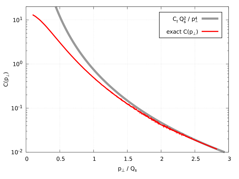
where $A_{a}^{+}(l\epsilon,{\bm{x}}_{\perp})$ is the solution of the discretized Poisson equation (3) in the slice $l$. In the rest of this paper, we use a square transverse lattice of size $N_{\perp}=64$ with spacing $Q_{s}a=1$, and $L=20$ slices in the $x^{-}$ direction. Furthermore, we consider $N_{c}=2$ just for simplicity of numerical calculations. In the figure 1, we show the result of evaluating the Fourier transform of the dipole amplitude in this setup, starting from a discrete version of eq. (2) (this result will later be referred to as “exact”, since the ensemble average is performed analytically), and we compare it to the asymptotic form (8).

Figure 1: Plot of the function $C(p_{\perp})$. Thin red line: based on a discrete version of eq. (6), on a $64\times 64\times 20$ lattice. The mass used in the infrared regularization is $m^{2}=0.2\,Q_{s}^{2}$. Thick gray band: asymptotic behavior $C_{{}_{F}}Q_{s}^{2}/p_{\perp}^{4}$.

3 Monte-Carlo evaluation without barycenter averaging

For the sake of the discussion, let us now assume that we do not know the analytical expression of eq. (6). Instead, we wish to obtain the 2-point function by a Monte-Carlo sampling of the Gaussian distribution of the sources $\rho_{a}$. In this section, we first consider numerical estimates of the dipole amplitude that evaluate the two-point function with one coordinate fixed at the origin of the transverse lattice, as defined in eq. (4).

3.1 Definition and basic properties

We draw randomly (within the statistical ensemble defined by eqs. (1)) $N$ configurations $\rho_{i,a}$ ($1\leq i\leq N$) of the source, and the exact analytical formula (6) and its Fourier transform are replaced by

$$C_{{}_{N}}({\bm{x}}_{\perp},0)\equiv\frac{1}{N}\sum_{i=1}^{N}{\frac{1}{N_{c}}\;{\rm tr}\,\left(U_{i}({\bm{x}}_{\perp})U^{\dagger}_{i}(0_{\perp})\right)}$$

$$C_{{}_{N}}({\bm{p}}_{\perp})\equiv\int d^{2}{\bm{x}}_{\perp}\;e^{i{\bm{p}}_{\perp}\cdot{\bm{x}}_{\perp}}\;C_{{}_{N}}({\bm{x}}_{\perp},0)\;,$$ (14)

where $U_{i}({\bm{x}}_{\perp})$ is a Wilson line calculated with the source $\rho_{i,a}$. (We use continuous notations for the Fourier transform for simplicity, but all the plots shown in the paper use a lattice discretization and a discrete Fourier transform, as explained in the previous section.) In the following, we will call $C_{{}_{N}}({\bm{p}}_{\perp})$ a measurement of $C({\bm{p}}_{\perp})$ with statistics $N$.

$C_{{}_{N}}({\bm{p}}_{\perp})$ is itself a random quantity, since it is obtained from a finite number $N$ of samples of the random source $\rho_{a}$. However, if we repeat many times the measurement defined in eq. (14), the mean value of the quantity $C_{{}_{N}}({\bm{p}}_{\perp})$ is the expected correlator $C({\bm{p}}_{\perp})$:

$$\left<C_{{}_{N}}({\bm{p}}_{\perp})\right>=C({\bm{p}}_{\perp}).$$ (15)

In this equation and in the following, the angle brackets $\langle\cdots\rangle$ indicate a statistical average over repeated measurements of the quantity contained between the brackets. This indicates that $C_{{}_{N}}({\bm{p}}_{\perp})$ fluctuates around the exact result $C({\bm{p}}_{\perp})$. Furthermore, when $N\to\infty$, these fluctuations should decrease thanks to the property

$$\lim_{N\to\infty}C_{{}_{N}}({\bm{p}}_{\perp})=C({\bm{p}}_{\perp}).$$ (16)

In other words, a single measurement with infinitely large statistics should also yield the exact answer.

In the previous section, we have mentioned the fact that exact correlation function $C({\bm{p}}_{\perp})$ is real valued thanks to the symmetry of the ensemble of color sources under ${\bm{x}}_{\perp}\to-{\bm{x}}_{\perp}$. However, this symmetry is not true event by event, and therefore measurements $C_{{}_{N}}({\bm{p}}_{\perp})$ with finite statistics are complex valued. In the limit of a large number of samples, $N\to\infty$, we have the following results,

$$\lim_{N\to\infty}C_{{}_{N}}({\bm{p}}_{\perp}) =C({\bm{p}}_{\perp}),$$

$$\lim_{N\to\infty}{\rm Re}\,C_{{}_{N}}({\bm{p}}_{\perp}) =C({\bm{p}}_{\perp}),$$

$$\lim_{N\to\infty}{\rm Im}\,C_{{}_{N}}({\bm{p}}_{\perp}) =0,$$

$$\lim_{N\to\infty}\big{|}C_{{}_{N}}({\bm{p}}_{\perp})\big{|} =C({\bm{p}}_{\perp}).$$ (17)

Therefore, we may use any of $C_{{}_{N}}$, ${\rm Re}\,C_{{}_{N}}$ or $\big{|}C_{{}_{N}}\big{|}$ as Monte-Carlo approximations of the exact result $C$. If we insist on a real-valued approximation, then ${\rm Re}\,C_{{}_{N}}$ or $\big{|}C_{{}_{N}}\big{|}$ should be considered.

Moreover, the ensemble of sources defined by eqs. (1) is invariant under rotations in the transverse plane, implying that the exact correlation function $C({\bm{p}}_{\perp})$ in fact depends only on the norm of the transverse momentum $p_{\perp}\equiv|{\bm{p}}_{\perp}|$. Again, this is a symmetry which is not realized event-by-event and therefore the above Monte-Carlo measurements are not rotationally invariant. We may enforce a rotationally invariant result by performing in addition an average over the orientation of ${\bm{p}}_{\perp}$ in the transverse plane, by using one of the following definitions

$$\big{(}{\rm Re}\,C_{{}_{N}}({\bm{p}}_{\perp})\big{)}_{\theta} \equiv\int\frac{d\theta}{2\pi}\;{\rm Re}\,C_{{}_{N}}({\bm{p}}_{\perp}),$$

$$\big{(}\big{|}C_{{}_{N}}({\bm{p}}_{\perp})\big{|}\big{)}_{\theta} \equiv\int\frac{d\theta}{2\pi}\;\big{|}C_{{}_{N}}({\bm{p}}_{\perp})\big{|},$$

$$\big{(}\big{|}C_{{}_{N}}({\bm{p}}_{\perp})\big{|}^{2}\big{)}_{\theta}^{1/2} \equiv\Big{[}\int\frac{d\theta}{2\pi}\;\big{|}C_{{}_{N}}({\bm{p}}_{\perp})\big{|}^{2}\Big{]}^{1/2}.$$ (18)

(Here also, we use a continuous notation for the integration over $\theta$, but in the lattice implementation this average is in fact a sum over the finite set of momenta that have a common norm (12).) When considering the angular average of the modulus, two definitions are possible, corresponding to the second or third of eqs. (18). In the rest of this paper, we are using the third equation, but we have checked that both definitions behave very similarly. Note also that this angular averaging eliminates the imaginary part of $C_{{}_{N}}({\bm{p}}_{\perp})$. Indeed, this average restores the symmetry ${\bm{x}}_{\perp}\to-{\bm{x}}_{\perp}$ even for a finite number of samples, leading to

$$\big{(}{\rm Im}\,C_{{}_{N}}({\bm{p}}_{\perp})\big{)}_{\theta}=0,\quad\big{(}{\rm Re}\,C_{{}_{N}}({\bm{p}}_{\perp})\big{)}_{\theta}=\big{(}C_{{}_{N}}({\bm{p}}_{\perp})\big{)}_{\theta}.$$ (19)

In the figure 2, we show the angular averaged values of $C_{{}_{N}}({\bm{p}}_{\perp})$, as well as the third of eqs. (18), with $N=10^{3}$. Although this is not shown in the plot in order to reduce clutter, we have checked that the angular averaging has only a mild effect in reducing the dispersion of the displayed quantities (expect of course for the imaginary part of $C_{{}_{N}}$, which is totally canceled by the averaging).

Figure 2: Angular averaged values of a measurement $C_{{}_{N}}({\bm{p}}_{\perp})$ for $N=10^{3}$ (circles), on a $64\times 64$ lattice. Triangles: values of $\big{(}\big{|}C_{{}_{N}}({\bm{p}}_{\perp})\big{|}^{2}\big{)}_{\theta}^{1/2}$, for the same number of samples. Solid line: exact value of $C({\bm{p}}_{\perp})$ on the same lattice.

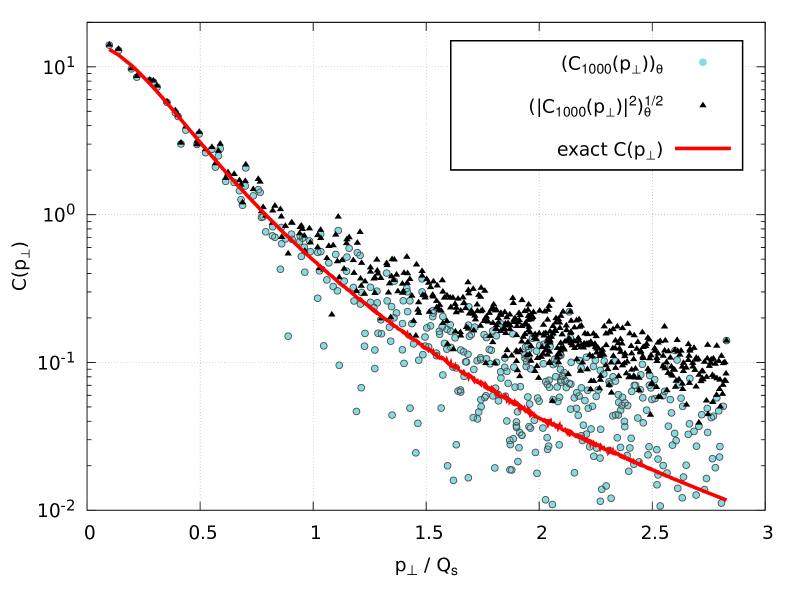
The first observation one may draw from this plot is the large scatter of the values of $\big{(}C_{{}_{N}}({\bm{p}}_{\perp})\big{)}_{\theta}$, despite the large number of samples used in the measurement. Another striking aspect is that the dispersion of the points increases relatively to the magnitude of the exact result as the momentum increases. In fact, at large momentum, this dispersion is so large that even the order of magnitude of the Monte-Carlo estimate is poorly controlled.

Consider now the triangles, that show the values of $\big{(}\big{|}C_{{}_{N}}({\bm{p}}_{\perp})\big{|}^{2}\big{)}_{\theta}^{1/2}$. At first sight, they appear to have a significantly lower dispersion compared to $\big{(}C_{{}_{N}}({\bm{p}}_{\perp})\big{)}_{\theta}$. If we did not know the exact answer, this might mislead us into thinking that $\big{(}\big{|}C_{{}_{N}}({\bm{p}}_{\perp})\big{|}^{2}\big{)}_{\theta}^{1/2}$ ought to provide a better approximation. However, since in this example we also know the exact result, the comparison quickly dissipates this hope: indeed, the plot readily shows that $\big{(}\big{|}C_{{}_{N}}({\bm{p}}_{\perp})\big{|}^{2}\big{)}_{\theta}^{1/2}$ fluctuates around a mean value that differ significantly from the exact result (in fact, it even has a tail that behaves as a different power of momentum).

In the rest of this section, we explain these observations by studying the statistical distribution of the values of $C_{{}_{N}}({\bm{p}}_{\perp})$ and $\big{|}C_{{}_{N}}({\bm{p}}_{\perp})\big{|}^{2}$.

3.2 Statistical fluctuations of $C_{{}_{N}}({\bm{p}}_{\perp})$

In order to estimate the statistical error made when we replace $C({\bm{p}}_{\perp})$ by a single measurement $C_{{}_{N}}({\bm{p}}_{\perp})$, let us consider the following variance

$$\sigma_{{}_{N}}^{2}({\bm{p}}_{\perp})\equiv\big{<}\big{|}C_{{}_{N}}({\bm{p}}_{\perp})-C({\bm{p}}_{\perp})\big{|}^{2}\big{>}=\big{<}\big{|}C_{{}_{N}}({\bm{p}}_{\perp})\big{|}^{2}\big{>}-C^{2}({\bm{p}}_{\perp}).$$ (20)

(We use the squared modulus $(C_{{}_{N}}-C)(C_{{}_{N}}-C)^{*}$ in order to have a real positive definite result despite the fact that $C_{{}_{N}}$ is complex-valued.) This quantity can also be written as

$$\sigma_{{}_{N}}^{2}({\bm{p}}_{\perp})=\big{<}\big{(}{\rm Re}\,C_{{}_{N}}({\bm{p}}_{\perp})\big{)}^{2}\big{>}-\big{<}{\rm Re}\,C_{{}_{N}}({\bm{p}}_{\perp})\big{>}^{2}+\big{<}\big{(}{\rm Im}\,C_{{}_{N}}({\bm{p}}_{\perp})\big{)}^{2}\big{>}-{\underbrace{\big{<}{\rm Im}\,C_{{}_{N}}({\bm{p}}_{\perp})\big{>}}_{0}}^{2}.$$ (21)

In other words, this quantity is the sum of the variances of the real part and of the imaginary part of $C_{{}_{N}}({\bm{p}}_{\perp})$. Note also that we have not included an angular average in the definition of this variance, for simplicity (the quantity defined in eq. (20) can be evaluated analytically). It nevertheless provides a good estimate of the fluctuations of $\big{(}C_{{}_{N}}({\bm{p}}_{\perp})\big{)}_{\theta}$, as we shall see shortly.

Let us first rewrite this variance in terms of correlators in coordinate space,

$$\sigma_{{}_{N}}^{2}({\bm{p}}_{\perp})=\int d^{2}{\bm{x}}_{\perp}d^{2}{\bm{y}}_{\perp}\;e^{i{\bm{p}}_{\perp}\cdot({\bm{x}}_{\perp}-{\bm{y}}_{\perp})}\;\Big{[}\big{<}C_{{}_{N}}({\bm{x}}_{\perp})C_{{}_{N}}^{*}({\bm{y}}_{\perp})\big{>}-\big{<}C_{{}_{N}}({\bm{x}}_{\perp})\big{>}\big{<}C_{{}_{N}}^{*}({\bm{y}}_{\perp})\big{>}\Big{]}.$$ (22)

In order to evaluate the ensemble average of $C_{{}_{N}}({\bm{x}}_{\perp})C_{{}_{N}}^{*}({\bm{y}}_{\perp})$, we first need to generalize the third of eqs. (1) into

$$\big{<}\rho_{i,a}(x^{-},{\bm{x}}_{\perp})\rho_{j,b}(y^{-},{\bm{y}}_{\perp})\big{>}=\mu^{2}(x^{-})\,\delta_{ij}\,\delta_{ab}\delta(x^{-}-y^{-})\delta({\bm{x}}_{\perp}-{\bm{y}}_{\perp}).$$ (23)

In other words, two configurations $i$ and $j$ of the source are not correlated if $i\not=j$, and if $i=j$ they are correlated as per the usual CGC prescription. Then, we have

$$\left<C_{{}_{N}}({\bm{x}}_{\perp})C_{{}_{N}}^{*}({\bm{y}}_{\perp})\right> =\frac{1}{N^{2}}\sum_{i,j}\frac{1}{N_{c}^{2}}\big{<}{\rm tr}\,(U_{i}({\bm{x}}_{\perp})U^{\dagger}_{i}(0_{\perp}))\;{\rm tr}\,(U^{\dagger}_{j}({\bm{y}}_{\perp})U_{j}(0_{\perp}))\big{>}$$

$$=\frac{1}{N^{2}}\!\!\sum_{i\not=j}\frac{1}{N_{c}^{2}}\big{<}{\rm tr}\,(U_{i}({\bm{x}}_{\perp})U^{\dagger}_{i}(0_{\perp}))\big{>}\big{<}{\rm tr}\,(U^{\dagger}_{j}({\bm{y}}_{\perp})U_{j}(0_{\perp}))\big{>}$$

$$+\frac{1}{N^{2}}\sum_{i}\frac{1}{N_{c}^{2}}\big{<}{\rm tr}\,(U_{i}({\bm{x}}_{\perp})U^{\dagger}_{i}(0_{\perp}))\;{\rm tr}\,(U^{\dagger}_{i}({\bm{y}}_{\perp})U_{i}(0_{\perp}))\big{>}$$

$$=\left(1-\frac{1}{N}\right)\,C({\bm{x}}_{\perp})\,C({\bm{y}}_{\perp})+\frac{1}{N}\,{\bm{\Sigma}}_{4}({\bm{x}}_{\perp},{\bm{y}}_{\perp}),$$ (24)

where we have defined

$${\bm{\Sigma}}_{4}({\bm{x}}_{\perp},{\bm{y}}_{\perp})\equiv\frac{1}{N_{c}^{2}}\big{<}{\rm tr}\,(U({\bm{x}}_{\perp})U^{\dagger}(0_{\perp}))\;{\rm tr}\,(U^{\dagger}({\bm{y}}_{\perp})U(0_{\perp}))\big{>}.$$ (25)

The variance $\sigma_{{}_{N}}^{2}({\bm{p}}_{\perp})$ thus reads

$$\sigma_{{}_{N}}^{2}({\bm{p}}_{\perp})=\frac{1}{N}\int d^{2}{\bm{x}}_{\perp}d^{2}{\bm{y}}_{\perp}\;e^{i{\bm{p}}_{\perp}\cdot({\bm{x}}_{\perp}-{\bm{y}}_{\perp})}\;\Big{[}{\bm{\Sigma}}_{4}({\bm{x}}_{\perp},{\bm{y}}_{\perp})-C({\bm{x}}_{\perp})C({\bm{y}}_{\perp})\Big{]},$$ (26)

and unsurprisingly it decreases as $1/N$ when the number of samples increases.

A general method for evaluating this type of correlation function in the MV model can be found in the appendix A of ref. [17]. When applied to eq. (25), this method leads to the following expression

$${\bm{\Sigma}}_{4}({\bm{x}}_{\perp},{\bm{y}}_{\perp})=\left(1-\frac{1}{N_{c}^{2}}\right)\;e^{\lambda_{+}}+\frac{1}{N_{c}^{2}}\;e^{\lambda_{-}},$$ (27)

with

$$\lambda_{+}\equiv\frac{N_{c}\,(\ell_{x0}+\ell_{0y})}{2}-\frac{\ell_{xy}}{2N_{c}},\quad\lambda_{-}\equiv C_{{}_{F}}\,\ell_{xy},$$

$$\mbox{and}\quad\ell_{xy}\equiv Q_{s}^{2}\int\frac{d^{2}{\bm{p}}_{\perp}}{(2\pi)^{2}}\;\frac{e^{i{\bm{p}}_{\perp}\cdot({\bm{x}}_{\perp}-{\bm{y}}_{\perp})}-1}{p_{\perp}^{4}}.$$ (28)

Note that these formulas are considerably simpler than those for a completely general 4-point correlator of Wilson lines (see the subsection 4.2 for the general case), thanks to the fact that two of the points in eq. (25) coincide.

3.2.1 Large $N_{c}$ limit

In the limit of a large number of colors, we can neglect all the terms that are suppressed by inverse powers of $N_{c}$, which leads to

$${\bm{\Sigma}}_{4}({\bm{x}}_{\perp},{\bm{y}}_{\perp})\mathrel{\mathop{\kern 0.0pt\approx}\limits_{N_{c}\gg 1}}e^{\lambda_{+}}$$

$$\lambda_{+}\mathrel{\mathop{\kern 0.0pt\approx}\limits_{N_{c}\gg 1}}\frac{N_{c}\,(\ell_{x0}+\ell_{0y})}{2}\;.$$ (29)

In this limit, ${\bm{\Sigma}}_{4}({\bm{x}}_{\perp},{\bm{y}}_{\perp})$ factorizes into the product of a function of ${\bm{x}}_{\perp}$ and a function of ${\bm{y}}_{\perp}$,

$${\bm{\Sigma}}_{4}({\bm{x}}_{\perp},{\bm{y}}_{\perp})\mathrel{\mathop{\kern 0.0pt\approx}\limits_{N_{c}\gg 1}}C({\bm{x}}_{\perp})C({\bm{y}}_{\perp})\;,$$ (30)

and the variance $\sigma_{{}_{N}}({\bm{p}}_{\perp})$ vanishes in the large $N_{c}$ limit. In other words, in the limit of a large number of colors, a single configuration of the source $\rho_{a}$ is sufficient in order to obtain the correct average over the sources. This is not surprising since there are no correlations between different colors in the MV ensemble: generating a single $\rho_{a}$ with many color components has the same effect as generating many configurations at finite $N_{c}$.

3.2.2 Finite $N_{c}$

The second term of eq. (27) is particularly interesting because it couples in a simple way the points ${\bm{x}}_{\perp}$ and ${\bm{y}}_{\perp}$. After Fourier transform, this term gives the following contribution to $\sigma_{{}_{N}}^{2}({\bm{p}}_{\perp})$,

$$\frac{1}{N\,N_{c}^{2}}\;{\cal S}_{\perp}\;C({\bm{p}}_{\perp}),$$ (31)

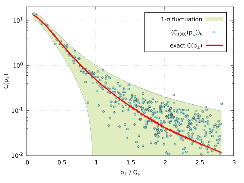
where ${\cal S}_{\perp}$ is the transverse area of the system under consideration (in order to see this, one should rewrite the integrals over ${\bm{x}}_{\perp},{\bm{y}}_{\perp}$ as integrals over the difference ${\bm{x}}_{\perp}-{\bm{y}}_{\perp}$ and barycenter $({\bm{x}}_{\perp}+{\bm{y}}_{\perp})/2$ – it is the latter that gives the factor ${\cal S}_{\perp}$). A crucial property of this term is that its behavior at large ${\bm{p}}_{\perp}$ ($\sim p_{\perp}^{-4}$) differs from that of the squared exact result $C^{2}({\bm{p}}_{\perp})\sim p_{\perp}^{-8}$. Therefore, the statistical errors are comparatively very large in the tail of the function $C({\bm{p}}_{\perp})$, to a point that makes this Monte-Carlo evaluation worthless with any reasonable number of samples. To illustrate this discussion, we show again in the figure 3 the estimate of $C({\bm{p}}_{\perp})$ from one measurement $\big{(}C_{{}_{N}}({\bm{p}}_{\perp})\big{)}_{\theta}$ with $N=10^{3}$, superimposed over a band whose boundaries are $C({\bm{p}}_{\perp})\pm\sigma_{{}_{N}}({\bm{p}}_{\perp})$ (with $\sigma_{{}_{N}}({\bm{p}}_{\perp})$ evaluated numerically from eqs. (26), (27) and (28)).

Figure 3: Monte-Carlo evaluation of the function $C(p_{\perp})$ from $\big{(}C_{{}_{N}}({\bm{p}}_{\perp})\big{)}_{\theta}$. Shaded band: one-sigma statistical fluctuation of $C_{{}_{N}}({\bm{p}}_{\perp})$ obtained form eqs. (26), (27) and (28). Solid line: exact result based on eq. (6). Circles: result of a single measurement of $\big{(}C_{{}_{N}}({\bm{p}}_{\perp})\big{)}_{\theta}$ with $N=10^{3}$ configurations.

3.3 Statistical fluctuations of $\big{(}|C_{{}_{N}}|^{2}\big{)}_{\theta}^{1/2}$

In the figure 4, we show the result of a single measurement of $\big{(}|C_{{}_{N}}|^{2}\big{)}_{\theta}^{1/2}$ with $N=10^{3}$ configurations of the sources $\rho_{a}$. As already mentioned, this quantity appears much less noisy than the estimate based on $\big{(}C_{{}_{N}}({\bm{p}}_{\perp})\big{)}_{\theta}$ shown in the previous figures. This can be understood from the variance of $\big{(}|C_{{}_{N}}|^{2}\big{)}_{\theta}^{1/2}$

$$\big{<}\big{(}|C_{{}_{N}}|^{2}\big{)}_{\theta}\big{>}-\big{<}\big{(}|C_{{}_{N}}|^{2}\big{)}_{\theta}^{1/2}\big{>}^{2},$$ (32)

that we have indicated in the figure 4 by a shaded area. Here, we have estimated eq. (32) by a Monte-Carlo sampling, i.e. by performing $M\gg 1$ (in the figure, we have used $M=2000$) successive measurements of the quantity $\big{(}|C_{{}_{N}}|^{2}\big{)}_{\theta}^{1/2}$. These $M$ measurements have also been used to compute the mean value of $\big{(}|C_{{}_{N}}|^{2}\big{)}_{\theta}^{1/2}$, shown by the orange points in the figure.

This variance clearly confirms that $\big{(}|C_{{}_{N}}|^{2}\big{)}_{\theta}^{1/2}$ provides an estimate of the 2-point correlator that fluctuates much less than those based on $\big{(}C_{{}_{N}}\big{)}_{\theta}$ itself. However, the figure also shows clearly that the mean value of $\big{(}|C_{{}_{N}}|^{2}\big{)}_{\theta}^{1/2}$ differs substantially from the exact value, and in particular exhibits a different power law of momentum in the tail. This can be understood from eqs. (24), (27), (28) and (31).

Figure 4: Monte-Carlo evaluation of the function $C(p_{\perp})$ from $\big{(}|C_{{}_{N}}|^{2}\big{)}_{\theta}^{1/2}$. Shaded band: Monte-Carlo estimate of the one-sigma fluctuation of $\big{(}|C_{{}_{N}}|^{2}\big{)}_{\theta}^{1/2}$. Solid line: exact result based on eq. (6). Triangles: result of a single measurement of $\big{(}|C_{{}_{N}}|^{2}\big{)}_{\theta}^{1/2}$ with $N=10^{3}$ configurations. Orange dots: mean value of these measurements.

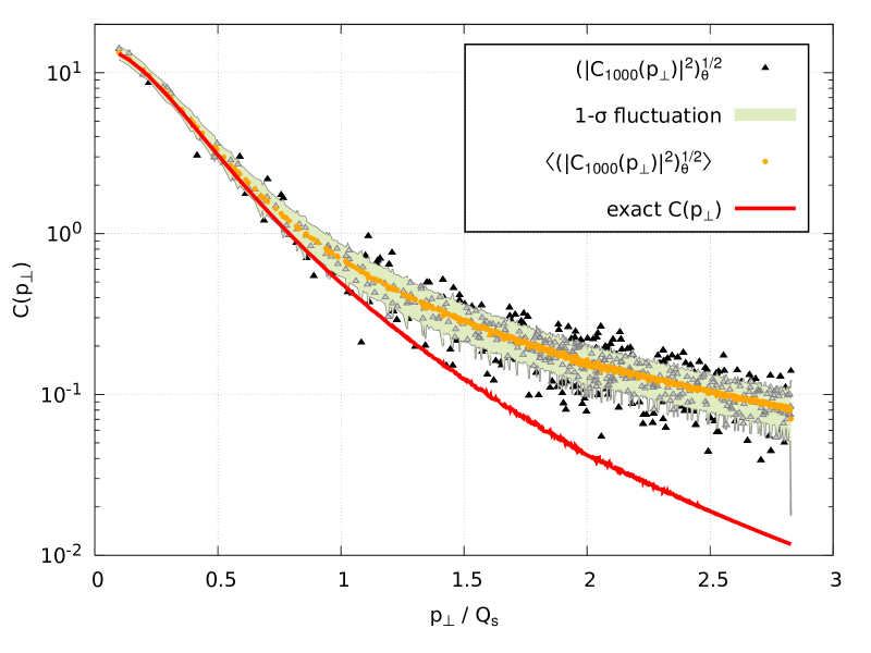
Indeed, these equations indicate that the mean value of $\big{|}C_{{}_{N}}({\bm{p}}_{\perp})\big{|}^{2}$ (this is not exactly the same quantity as the $\big{(}|C_{{}_{N}}|^{2}\big{)}_{\theta}$ considered in this subsection, but their tails have the same asymptotic behavior) contains a term in $N^{-1}p_{\perp}^{-4}$, while the exact answer for $C^{2}({\bm{p}}_{\perp})$ has a tail in $p_{\perp}^{-8}$. The measurement of $\big{(}|C_{{}_{N}}|^{2}\big{)}_{\theta}^{1/2}$ contains a contamination at large momentum that goes away rather slowly (like $N^{-1}$) with the number $N$ of source configurations used in each measurement. In other words, the comparatively small fluctuation of $\big{(}|C_{{}_{N}}|^{2}\big{)}_{\theta}^{1/2}$ is rather misleading, because it is not an indicator of its proximity with the correct value $C({\bm{p}}_{\perp})$.

4 Improvement by averaging over the barycenter

4.1 Definition

In the definition (4) of the 2-point function that we have used as example, one of the two points is fixed at the origin of the transverse plane. In this section, we shall discuss the improvement achieved by letting this point free and integrating it out, i.e. by generalizing the definition of the correlation function as follows

$$C({\bm{p}}_{\perp})\equiv\frac{1}{N_{c}}\frac{1}{{\cal S}_{\perp}}\int d^{2}{\bm{x}}_{\perp}d^{2}{\bm{y}}_{\perp}\;e^{i{\bm{p}}_{\perp}\cdot({\bm{x}}_{\perp}-{\bm{y}}_{\perp})}\;\left<{\rm tr}\,\left(U({\bm{x}}_{\perp})U^{\dagger}({\bm{y}}_{\perp})\right)\right>.$$ (33)

The two definitions are equivalent for a system invariant by translation. However, in a Monte-Carlo evaluation, they may differ with finite statistics since individual configurations of the sources are not translation invariant.

Interestingly, this averaging over the barycenter eliminates the imaginary part of Monte-Carlo estimates, even when the correlator is evaluated with a finite number of samples. Indeed, the complex conjugate of $C_{{}_{N}}({\bm{p}}_{\perp})$ reads

$$C_{{}_{N}}^{*}({\bm{p}}_{\perp}) =\frac{1}{NN_{c}{\cal S}_{\perp}}\sum_{i}\int d^{2}{\bm{x}}_{\perp}d^{2}{\bm{y}}_{\perp}\;e^{-i{\bm{p}}_{\perp}\cdot({\bm{x}}_{\perp}-{\bm{y}}_{\perp})}\;{\rm tr}\,\left((U_{i}({\bm{x}}_{\perp})U^{\dagger}_{i}({\bm{y}}_{\perp}))^{\dagger}\right)$$

$$=\frac{1}{NN_{c}{\cal S}_{\perp}}\sum_{i}\int d^{2}{\bm{x}}_{\perp}d^{2}{\bm{y}}_{\perp}\;e^{-i{\bm{p}}_{\perp}\cdot({\bm{x}}_{\perp}-{\bm{y}}_{\perp})}\;{\rm tr}\,\left(U_{i}({\bm{y}}_{\perp})U^{\dagger}_{i}({\bm{x}}_{\perp})\right)$$

$$=\frac{1}{NN_{c}{\cal S}_{\perp}}\sum_{i}\int d^{2}{\bm{x}}_{\perp}d^{2}{\bm{y}}_{\perp}\;e^{i{\bm{p}}_{\perp}\cdot({\bm{x}}_{\perp}-{\bm{y}}_{\perp})}\;{\rm tr}\,\left(U_{i}({\bm{x}}_{\perp})U^{\dagger}_{i}({\bm{y}}_{\perp})\right)$$

$$=C_{{}_{N}}({\bm{p}}_{\perp})\;.$$ (34)

Note that the manipulations performed here are only possible because we are integrating on both ${\bm{x}}_{\perp}$ and ${\bm{y}}_{\perp}$.

Figure 5: Monte-Carlo evaluation of the function $C(p_{\perp})$ from $\big{(}C_{{}_{N}}({\bm{p}}_{\perp})\big{)}_{\theta}$, with barycenter and angular averaging. Solid line: exact result based on eq. (6). Circles: result of a single measurement of $C_{{}_{N}}({\bm{p}}_{\perp})$ with only ten ($N=10$) configurations.

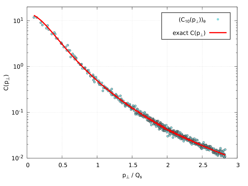
In the figure 5, we show the estimate of $C({\bm{p}}_{\perp})$ from the value of $\big{(}C_{{}_{N}}({\bm{p}}_{\perp})\big{)}_{\theta}$, for $N=10$, using the barycenter averaging described in this section. One can see that despite the small number of configurations used in this computation, this estimate tracks remarkably well the exact result. Naturally, one naively expects that the barycenter averaging roughly amounts to increasing the statistics by a factor equal to the number of lattice sites, i.e. by a factor $64\times 64=4096$ in the present case. But the figure also suggests that the momentum dependence of the fluctuations has changed, in such a way that the relative error is now independent of momentum.

4.2 Statistical fluctuations

4.2.1 Analytical expression

The momentum dependence of the fluctuations in measurements using barycenter averaging can be understood by calculating the corresponding variance. With barycenter averaging, the mean value of $C_{{}_{N}}^{2}({\bm{p}}_{\perp})$ reads

$$\big{<}C_{{}_{N}}^{2}({\bm{p}}_{\perp})\big{>}=\left(1-\frac{1}{N}\right)\,C^{2}({\bm{p}}_{\perp})+\frac{1}{N}\,{\bm{\Sigma}}_{4}({\bm{p}}_{\perp}),$$ (35)

where we have defined

$${\bm{\Sigma}}_{4}({\bm{p}}_{\perp}) \equiv\frac{1}{{\cal S}_{\perp}^{2}}\int d^{2}{\bm{x}}_{\perp}d^{2}{\bm{y}}_{\perp}d^{2}{\bm{u}}_{\perp}d^{2}{\bm{v}}_{\perp}\;e^{i{\bm{p}}_{\perp}\cdot({\bm{x}}_{\perp}-{\bm{y}}_{\perp})}e^{i{\bm{p}}_{\perp}\cdot({\bm{u}}_{\perp}-{\bm{v}}_{\perp})}$$

$$\qquad\qquad\qquad\times\underbrace{\tfrac{1}{N_{c}^{2}}\left<{\rm tr}\,\big{(}U({\bm{x}}_{\perp})U^{\dagger}({\bm{y}}_{\perp})\big{)}\;{\rm tr}\,\big{(}U({\bm{u}}_{\perp})U^{\dagger}({\bm{v}}_{\perp})\big{)}\right>}_{{\bm{\Sigma}}_{4}({\bm{x}}_{\perp}{\bm{y}}_{\perp};{\bm{u}}_{\perp}{\bm{v}}_{\perp})}.$$ (36)

Using the method described in the appendix A of ref. [17], we obtain

$${\bm{\Sigma}}_{4}({\bm{x}}_{\perp}{\bm{y}}_{\perp};{\bm{u}}_{\perp}{\bm{v}}_{\perp})=A_{+}\;e^{\lambda_{+}}+A_{-}\;e^{\lambda_{-}}\;,$$ (37)

with

$$A_{\pm} \equiv\frac{1}{2}\pm\frac{1}{\sqrt{\Delta}}\left(\frac{N_{c}(\alpha-\beta)}{2}+\frac{\beta-\gamma}{N_{c}}\right)$$

$$\lambda_{\pm} \equiv\frac{N_{c}(\alpha+\beta)}{4}+\frac{\gamma-\alpha-\beta}{2N_{c}}\pm\frac{\sqrt{\Delta}}{4}$$

$$\Delta \equiv N_{c}^{2}(\alpha-\beta)^{2}+4(\alpha-\gamma)(\beta-\gamma)$$

$$\alpha \equiv\ell_{xy}+\ell_{uv}\;,\quad\beta\equiv\ell_{xv}+\ell_{yu}\;,\quad\gamma\equiv\ell_{xu}+\ell_{yv},$$ (38)

and $\ell_{xy}$ is the quantity defined in eq. (28).

4.2.2 Large $N_{c}$ limit

In the large $N_{c}$ limit, we have

$$\lambda_{+}\approx\frac{N_{c}}{2}\,{\rm max}\,(\alpha,\beta)\;,\quad\lambda_{-}\approx\frac{N_{c}}{2}\,{\rm min}\,(\alpha,\beta)$$

$$A_{\pm}\approx\frac{1}{2}(1\pm{\rm sign}\,(\alpha-\beta)),$$ (39)

and as a consequence we obtain

$${\bm{\Sigma}}_{4}({\bm{x}}_{\perp}{\bm{y}}_{\perp};{\bm{u}}_{\perp}{\bm{v}}_{\perp})\approx e^{\tfrac{Q_{s}^{2}N_{c}}{2}(\ell_{xy}+\ell_{uv})}\;.$$ (40)

After performing the Fourier transforms and inserting into eq. (35), this leads to a vanishing variance

$$\big{<}C_{{}_{N}}^{2}({\bm{p}}_{\perp})\big{>}-C^{2}({\bm{p}}_{\perp})\approx 0\;.$$ (41)

In other words, the fluctuations of $C_{{}_{N}}$ are suppressed by inverse powers of the number of colors, as was already the case when we did not perform any barycenter averaging.

4.2.3 Finite $N_{c}$

We thus need to keep $N_{c}$ finite in order to obtain a non trivial result for the variance. If we expand to order $N_{c}^{-2}$ the coefficients $A_{\pm}$, while keeping only the leading $N_{c}$ term in the eigenvalues $\lambda_{\pm}$, we obtain

$${\bm{\Sigma}}_{4}({\bm{x}}_{\perp}{\bm{y}}_{\perp};{\bm{u}}_{\perp}{\bm{v}}_{\perp})\approx e^{\tfrac{Q_{s}^{2}N_{c}}{2}(\ell_{xy}+\ell_{uv})}$$

$$\quad+\frac{1}{N_{c}^{2}}\left(\frac{\ell_{xv}+\ell_{yu}-\ell_{xu}-\ell_{yv}}{\ell_{xv}+\ell_{yu}-\ell_{xy}-\ell_{uv}}\right)^{2}\left(e^{\tfrac{N_{c}}{2}(\ell_{xv}+\ell_{yu})}-e^{\tfrac{N_{c}}{2}(\ell_{xy}+\ell_{uv})}\right),$$ (42)

so that the variance can be approximated by

$$\!\!\big{<}C_{{}_{N}}^{2}({\bm{p}}_{\perp})\big{>}-C^{2}({\bm{p}}_{\perp})\approx\frac{1}{NN_{c}^{2}}\int\frac{d^{2}{\bm{x}}_{\perp}d^{2}{\bm{y}}_{\perp}d^{2}{\bm{u}}_{\perp}d^{2}{\bm{v}}_{\perp}}{{\cal S}_{\perp}^{2}}\;e^{i{\bm{p}}_{\perp}\cdot({\bm{x}}_{\perp}-{\bm{y}}_{\perp}+{\bm{u}}_{\perp}-{\bm{v}}_{\perp})}$$

$$\qquad\quad\times\left(\frac{\ell_{xv}+\ell_{yu}-\ell_{xu}-\ell_{yv}}{\ell_{xv}+\ell_{yu}-\ell_{xy}-\ell_{uv}}\right)^{2}\left(e^{\tfrac{N_{c}}{2}(\ell_{xv}+\ell_{yu})}-e^{\tfrac{N_{c}}{2}(\ell_{xy}+\ell_{uv})}\right).$$ (43)

From this formula, one can understand the different behaviors of the variance with and without barycenter averaging. The integral in this formula depends on the transverse area ${\cal S}_{\perp}$, on the saturation momentum $Q_{s}$ and on the transverse momentum $p_{\perp}$, combined in such a way to give a result of mass dimension $-4$. The momentum ${\bm{p}}_{\perp}$ is the Fourier conjugate of the coordinate differences ${\bm{x}}_{\perp}-{\bm{y}}_{\perp}$ and ${\bm{u}}_{\perp}-{\bm{v}}_{\perp}$, or of ${\bm{x}}_{\perp}-{\bm{v}}_{\perp}$ and ${\bm{u}}_{\perp}-{\bm{y}}_{\perp}$. In this discussion, one can use the following approximation for the function $\ell_{xy}$,

$$\ell_{xy}\approx-\frac{Q_{s}^{2}({\bm{x}}_{\perp}-{\bm{y}}_{\perp})^{2}}{8\pi}\,\ln\left(\frac{a_{{}_{\rm IR}}}{|{\bm{x}}_{\perp}-{\bm{y}}_{\perp}|}\right)\;,$$ (44)

where $a_{{}_{\rm IR}}$ is an infrared cutoff (here introduced in the form of a distance such that $Q_{s}a_{{}_{\rm IR}}\gg 1$). For the sake of this argument, one can ignore the first factor in the second line of eq. (43), because its dependence on the coordinates is a rational fraction, while the second factor has an exponential dependence. For momenta $p_{\perp}\gtrsim Q_{s}$, the Fourier transform of $\exp(N_{c}\ell_{xy}/2)$ behaves as

$$\int d^{2}({\bm{x}}_{\perp}-{\bm{y}}_{\perp})\;e^{i{\bm{p}}_{\perp}\cdot({\bm{x}}_{\perp}-{\bm{y}}_{\perp})}\;e^{\tfrac{N_{c}}{2}\ell_{xy}}\sim\frac{Q_{s}^{2}}{p_{\perp}^{4}}\;.$$ (45)

Therefore, at large momentum, $Q_{s}^{2}/p_{\perp}^{4}$ is the only combination by which $Q_{s}$ and $p_{\perp}$ can enter in the variance. One should therefore count how many of these factors can arise (1 or 2), and add the appropriate factors of ${\cal S}_{\perp}$ to reach the dimension $-4$. In eq. (43), we see that there are two Fourier integrals with respect to coordinate differences, each of which brings a factor $Q_{s}^{2}/p_{\perp}^{4}$. The remaining two integrations are over the “barycenter” coordinates. Each of them brings a factor ${\cal S}_{\perp}$, and they cancel the factor ${\cal S}_{\perp}^{-2}$. Therefore, the formula (43) behaves as follows

$$\sqrt{\big{<}C_{{}_{N}}^{2}({\bm{p}}_{\perp})\big{>}-C^{2}({\bm{p}}_{\perp})}\sim\frac{1}{N_{c}\sqrt{N}}\;\frac{Q_{s}^{2}}{p_{\perp}^{4}}.$$ (46)

This explain why in the figure 5 the dispersion of the points appears to be a roughly constant fraction of the central value, since

$$\left.\frac{\sqrt{\big{<}C_{{}_{N}}^{2}({\bm{p}}_{\perp})\big{>}-C^{2}({\bm{p}}_{\perp})}}{C({\bm{p}}_{\perp})}\right|_{{\rm with\ barycenter}\atop{\rm averaging}}\sim\frac{1}{N_{c}\sqrt{N}}.$$ (47)

From the same starting point, eq. (43), it is easy to see what changes if we do not use barycenter averaging. In this case, the coordinates ${\bm{y}}_{\perp}$ and ${\bm{u}}_{\perp}$ are not integrated out but instead fixed to ${\bm{y}}_{\perp}={\bm{u}}_{\perp}=0_{\perp}$ (the denominator ${\cal S}_{\perp}^{2}$ also disappears if we do this). Therefore, we have $\ell_{yu}\equiv 0$, and one of the Fourier integrals disappears in the first term, which means that we get a single factor $Q_{s}^{2}/p_{\perp}^{4}$ and a factor ${\cal S}_{\perp}$ to make up for the correct dimension. In the end, we now get

$$\left.\frac{\sqrt{\big{<}C_{{}_{N}}^{2}({\bm{p}}_{\perp})\big{>}-C^{2}({\bm{p}}_{\perp})}}{C({\bm{p}}_{\perp})}\right|_{{\rm without\ barycenter}\atop{\rm averaging}}\sim\frac{1}{N_{c}\sqrt{N}}\;\sqrt{\frac{{\cal S}_{\perp}p_{\perp}^{4}}{Q_{s}^{2}}},$$ (48)

and the variance is increased by a (large) factor $\sqrt{{\cal S}_{\perp}}$. The absence of this factor ${\cal S}_{\perp}$ in eq. (47) is the reason why this procedure is called barycenter averaging (or self-averaging): the same configuration of sources provides an effective statistics enhanced by the number of lattice sites if we also average over the mid-point in the 2-point correlation function. But more importantly, if we do not perform this barycenter averaging, the momentum dependence of the variance differs from that of the mean value $C(p_{\perp})$ (it has a large momentum tail that decreases much slower), which leads to very important relative errors at large momentum.

5 Summary and conclusions

In this paper, we have studied the statistical errors encountered in the Monte-Carlo evaluation of the expectation value of correlation functions in the Color Glass Condensate, on the simple example of the dipole amplitude. Assuming a uniform saturation momentum, this correlator is invariant by translation in the transverse plane.

In a first series of Monte-Carlo estimates, we do not exploit the translation invariance and instead we pin one of the two coordinates to the origin of the transverse plane. A first “measurement” we have considered is simply to compute the correlator with $N$ samples of the color sources. We observed that this leads to a very noisy result –even with a rather large value of $N$– at high momentum, only marginally improved by averaging over the orientations of the transverse momentum. More importantly, the relative error appears to increase dramatically with momentum. This behavior was then explained by calculating the variance of such measurements.

More unexpected was the behavior of statistical fluctuations in the case of the modulus of the above Monte-Carlo estimate (still with one point at a fixed location on the lattice). With the same number $N$ of samples, it appears to be considerably less noisy, but also rather far from the exact answer – and with a relative discrepancy that increases with momentum. The calculation of the mean value of this measurement indicates that it indeed differs from the exact answer by a term of order $N^{-1}$, that dominates the large momentum tail.

Then, we turned to a measurement in which one also averages over the barycenter of the two points. In this case, the statistical errors are much lower even with a small number of samples, and in addition they appear to scale proportionally to the magnitude of the exact result – unlike the error encountered when one point of the correlator was held fixed. This improvement due to the averaging over the barycenter could be explained by studying the variance of these measurements.

Our study was centered on a very simple example, in order to have an exact answer to compare with and to be able to discuss semi-analytically the variance of the Monte-Carlo measurements. However, we expect our observations to be valid for any translation invariant CGC correlator, namely that the barycenter averaging reduces the relative statistical error of Monte-Carlo measurements by a factor $(Q_{s}^{2}/{\cal S}_{\perp}p_{\perp}^{4})^{1/2}$, where $p_{\perp}$ denotes generically the Fourier conjugate variable to a difference of coordinates. Therefore, our study should be viewed as a call for caution in the numerical evaluation of correlation functions in the CGC framework. The first message is that pinning a point of the correlator at a fixed location generally leads to significantly larger errors, especially at large momentum. In most of these measurements, the large statistical errors will be strikingly visible in the form of a very noisy output, as in the figure 3. But we also would like to warn the reader about the existence of alternate measurements –also without barycenter averaging–, where the statistical fluctuations appear to be much smaller and yet the result is equally incorrect, as in the figure 4. In other words, the “noisiness” of the results is not always a good measure of the error. In order to avoid these problems, the only safe way to limit the statistical errors in this type of measurement is to average the correlator over the barycenter of the points it involves.

References

- [1] Edmond Iancu, Andrei Leonidov, and Larry McLerran. The Color glass condensate: An Introduction. In QCD perspectives on hot and dense matter. Proceedings, NATO Advanced Study Institute, Summer School, Cargese, France, August 6-18, 2001, pages 73–145, 2002.
- [2] Heribert Weigert. Evolution at small x(bj): The Color glass condensate. Prog. Part. Nucl. Phys., 55:461–565, 2005.
- [3] Francois Gelis, Edmond Iancu, Jamal Jalilian-Marian, and Raju Venugopalan. The Color Glass Condensate. Ann. Rev. Nucl. Part. Sci., 60:463–489, 2010.
- [4] F. Gelis. Color Glass Condensate and Glasma. Int. J. Mod. Phys., A28:1330001, 2013.
- [5] Larry D. McLerran and Raju Venugopalan. Computing quark and gluon distribution functions for very large nuclei. Phys. Rev., D49:2233–2241, 1994.
- [6] Larry D. McLerran and Raju Venugopalan. Gluon distribution functions for very large nuclei at small transverse momentum. Phys. Rev., D49:3352–3355, 1994.
- [7] Jamal Jalilian-Marian, Alex Kovner, Andrei Leonidov, and Heribert Weigert. The BFKL equation from the Wilson renormalization group. Nucl. Phys., B504:415–431, 1997.
- [8] Jamal Jalilian-Marian, Alex Kovner, Andrei Leonidov, and Heribert Weigert. The Wilson renormalization group for low x physics: Towards the high density regime. Phys. Rev., D59:014014, 1998.
- [9] Edmond Iancu, Andrei Leonidov, and Larry D. McLerran. Nonlinear gluon evolution in the color glass condensate. 1. Nucl. Phys., A692:583–645, 2001.
- [10] Elena Ferreiro, Edmond Iancu, Andrei Leonidov, and Larry McLerran. Nonlinear gluon evolution in the color glass condensate. 2. Nucl. Phys., A703:489–538, 2002.
- [11] Alex Krasnitz and Raju Venugopalan. The Initial gluon multiplicity in heavy ion collisions. Phys. Rev. Lett., 86:1717–1720, 2001.
- [12] Alex Krasnitz, Yasushi Nara, and Raju Venugopalan. Coherent gluon production in very high-energy heavy ion collisions. Phys. Rev. Lett., 87:192302, 2001.
- [13] T. Lappi. Production of gluons in the classical field model for heavy ion collisions. Phys. Rev., C67:054903, 2003.
- [14] F. Gelis and A. Peshier. Probing colored glass via q anti-q photoproduction. Nucl. Phys., A697:879–901, 2002.
- [15] Francois Gelis and Jamal Jalilian-Marian. Photon production in high-energy proton nucleus collisions. Phys. Rev., D66:014021, 2002.
- [16] Kenji Fukushima. Randomness in infinitesimal extent in the McLerran-Venugopalan model. Phys. Rev., D77:074005, 2008.
- [17] Jean Paul Blaizot, Francois Gelis, and Raju Venugopalan. High-energy pA collisions in the color glass condensate approach. 2. Quark production. Nucl. Phys., A743:57–91, 2004.