A Structure-Preserving One-Sided Jacobi Method for Computing the SVD of a Quaternion Matrix

Ru-Ru Ma School of Mathematical Sciences, Xiamen University, Xiamen 361005, People’s Republic of China (maruru7271@126.com). The research of this author is partially supported by the Fundamental Research Funds for the Central Universities (No. 20720180008).    Zheng-Jian Bai Corresponding author. School of Mathematical Sciences and Fujian Provincial Key Laboratory on Mathematical Modeling & High Performance Scientific Computing, Xiamen University, Xiamen 361005, People’s Republic of China (zjbai@xmu.edu.cn). The research of this author is partially supported by the National Natural Science Foundation of China (No. 11671337), the Natural Science Foundation of Fujian Province of China (No. 2016J01035), and the Fundamental Research Funds for the Central Universities (No. 20720180008).
Abstract

In this paper, we provide a structure-preserving one-sided cyclic Jacobi method for computing the singular value decomposition of a quaternion matrix. In this method, the columns of the quaternion matrix are orthogonalized in pairs by using a sequence of orthogonal JRS-symplectic Jacobi matrices to its real counterpart. The quadratic convergence is also established under some mild conditions. Numerical tests are reported to illustrate the efficiency of the proposed method.

Keywords. Quaternion matrix; singular value decomposition; one-sided cyclic Jacobi method; Color image compression

AMS subject classifications. 65F18, 65F15, 15A18, 65K05, 90C26, 90C48

1 Introduction

The concept of quaternions was originally introduced by Hamilton [10]. Quaternions and quaternion matrices arise in various applications in applied science such as quaternionic quantum mechanics [1, 2, 6], color image processing [32] and field theory [19], etc. The quaternion matrix singular value decomposition (QSVD) was studied theoretically in 1997 by Zhang [35]. Recently, the QSVD has been an important tool in many applications such as color image processing [7, 17, 22, 24], signal processing [16, 33], and electroencephalography [5], etc.

Various numerical methods have been proposed for computing the QSVD. In [15, 16, 24], some algorithms were provided to calculate the singular value decomposition (SVD) of a quaternion matrix via utilizing its equivalent complex matrix. In [27], Sangwine and Le Bihan proposed a method for computing the QSVD based on bidiagonalization via quaternionic Householder transformations. In [18], Le Bihan and Sangwine gave an implicit Jacobi algorithm for computing the QSVD where the quaternion arithmetic is employed instead of a complex equivalent representation. In [3], Doukhnitch and Ozen presented a coordinate rotation digital computer algorithm for computing the QSVD.

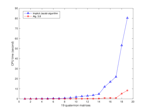
In this paper, we propose a structure-preserving one-sided cyclic Jacobi method for computing the QSVD. This is motivated by the recent structure-preserving methods related to quaternion matrices. In particular, Jia et al. designed a real structure-preserving method for quaternion Hermitian eigenvalue problems by using the structure-preserving tridiagonalization of the real counterpart for quaternion Hermitian matrices [11]. Li et al. presented a structure-preserving algorithm for computing the QSVD, which uses the structure-preserving bidiagonalization of the real counterpart of quaternion matrices via Householder-based transformations [20, 21]. Ma et al. proposed a structure-preserving Jacobi algorithm for quaternion Hermitian eigenvalue problems [23]. In this paper, the columns of a rectangle quaternion matrix are orthogonalized in pairs by using a sequence of orthogonal JRS-symplectic Jacobi matrices to its real counterpart. When the updated quaternion matrix has sufficiently orthogonal columns, the SVD is obtained by column scaling. Numerical experiments show that our method is more efficient than the implicit Jacobi algorithm in [18] and gives almost the same singular values as the solver in quaternion toolbox for MATLAB [26].

The rest of this paper is organized as follows. In section 2 we give necessary preliminaries used in this paper. In section 3 a structure-preserving one-sided cyclic Jacobi algorithm is provided for computing the QSVD and the quadratic convergence is established under some assumptions. In section 4 we report some numerical experiments to indicate the efficiency of our algorithm and apply it to color image compression. Finally, some concluding remarks are given in section 5.

2 Preliminaries

In this section, we briefly review some necessary definitions and properties of quaternions and quaternion matrices. Quaternions were originally introduced by Hamilton in 1843 [9]. For more information on quaternions, one may refer to [13, 35] and references therein.

Throughout this paper, we need the following notation. Let {\mathbb{R}} and m×nsuperscript𝑚𝑛{\mathbb{R}}^{m\times n} be the set of all real numbers and the set of all m×n𝑚𝑛m\times n real matrices respectively. Let \mathbb{H} and m×nsuperscript𝑚𝑛\mathbb{H}^{m\times n} be the set of all quaternions and the set of all m×n𝑚𝑛m\times n quaternion matrices respectively. Let Insubscript𝐼𝑛I_{n} be the identity matrix of order n𝑛n. Let AT,A¯superscript𝐴𝑇¯𝐴A^{T},\bar{A} and Asuperscript𝐴A^{*} stand for the transpose, conjugate and conjugate transpose of a matrix A𝐴A accordingly. F\|\cdot\|_{F} means the Frobenius matrix norm. For any n×n𝑛𝑛n\times n square matrix A=(apq)𝐴subscript𝑎𝑝𝑞A=(a_{pq}), we define

off(A):=p=1nq=1qpn|apq|2,assignoff𝐴superscriptsubscript𝑝1𝑛superscriptsubscript𝑞1𝑞𝑝𝑛superscriptsubscript𝑎𝑝𝑞2{\rm off}(A):=\sqrt{\sum\limits_{p=1}^{n}\sum\limits_{\begin{subarray}{c}q=1\\ q\neq p\end{subarray}}^{n}|a_{pq}|^{2}},

where |apq|subscript𝑎𝑝𝑞|a_{pq}| denotes the absolute value of apqsubscript𝑎𝑝𝑞a_{pq}.

A quaternion a𝑎a\in\mathbb{H} takes the form of

a=a0+a1i+a2j+a3k,𝑎subscript𝑎0subscript𝑎1𝑖subscript𝑎2𝑗subscript𝑎3𝑘a=a_{0}+a_{1}i+a_{2}j+a_{3}k,

where a0,a1,a2,a3subscript𝑎0subscript𝑎1subscript𝑎2subscript𝑎3a_{0},a_{1},a_{2},a_{3}\in\mathbb{R} and the quaternion units i,j,k𝑖𝑗𝑘i,j,k satisfy the following rules

i2=j2=k2=1,jk=kj=i,ki=ik=j,ij=ji=k.formulae-sequencesuperscript𝑖2superscript𝑗2superscript𝑘21𝑗𝑘𝑘𝑗𝑖𝑘𝑖𝑖𝑘𝑗𝑖𝑗𝑗𝑖𝑘i^{2}=j^{2}=k^{2}=-1,\quad jk=-kj=i,\quad ki=-ik=j,\quad ij=-ji=k.

The conjugate of a𝑎a\in\mathbb{H} is given by a¯=a=a0a1ia2ja3k¯𝑎superscript𝑎subscript𝑎0subscript𝑎1𝑖subscript𝑎2𝑗subscript𝑎3𝑘\bar{a}=a^{*}=a_{0}-a_{1}i-a_{2}j-a_{3}k. For two quaternions a=a0+a1i+a2j+a3k𝑎subscript𝑎0subscript𝑎1𝑖subscript𝑎2𝑗subscript𝑎3𝑘a=a_{0}+a_{1}i+a_{2}j+a_{3}k\in\mathbb{H} and b=b0+b1i+b2j+b3k𝑏subscript𝑏0subscript𝑏1𝑖subscript𝑏2𝑗subscript𝑏3𝑘b=b_{0}+b_{1}i+b_{2}j+b_{3}k\in\mathbb{H}, their product (i.e., the Hamilton product) is given by

ab𝑎𝑏\displaystyle ab =\displaystyle= a0b0a1b1a2b2a3b3subscript𝑎0subscript𝑏0subscript𝑎1subscript𝑏1subscript𝑎2subscript𝑏2subscript𝑎3subscript𝑏3\displaystyle a_{0}b_{0}-a_{1}b_{1}-a_{2}b_{2}-a_{3}b_{3}
+(a0b1+a1b0+a2b3a3b2)isubscript𝑎0subscript𝑏1subscript𝑎1subscript𝑏0subscript𝑎2subscript𝑏3subscript𝑎3subscript𝑏2𝑖\displaystyle+(a_{0}b_{1}+a_{1}b_{0}+a_{2}b_{3}-a_{3}b_{2})i
+(a0b2a1b3+a2b0+a3b1)jsubscript𝑎0subscript𝑏2subscript𝑎1subscript𝑏3subscript𝑎2subscript𝑏0subscript𝑎3subscript𝑏1𝑗\displaystyle+(a_{0}b_{2}-a_{1}b_{3}+a_{2}b_{0}+a_{3}b_{1})j
+(a0b3+a1b2a2b1+a3b0)k.subscript𝑎0subscript𝑏3subscript𝑎1subscript𝑏2subscript𝑎2subscript𝑏1subscript𝑎3subscript𝑏0𝑘\displaystyle+(a_{0}b_{3}+a_{1}b_{2}-a_{2}b_{1}+a_{3}b_{0})k.

The absolute value |a|𝑎|a| of a=a0+a1i+a2j+a3k𝑎subscript𝑎0subscript𝑎1𝑖subscript𝑎2𝑗subscript𝑎3𝑘a=a_{0}+a_{1}i+a_{2}j+a_{3}k\in\mathbb{H} is defined by

|a|=a02+a12+a22+a32=aa¯=a¯a.𝑎superscriptsubscript𝑎02superscriptsubscript𝑎12superscriptsubscript𝑎22superscriptsubscript𝑎32𝑎¯𝑎¯𝑎𝑎|a|=\sqrt{a_{0}^{2}+a_{1}^{2}+a_{2}^{2}+a_{3}^{2}}=\sqrt{a\bar{a}}=\sqrt{\bar{a}a}.

The multiplicative inverse of any nonzero quaternion 0a0𝑎0\neq a\in\mathbb{H} is given by a1=a¯/|a|2superscript𝑎1¯𝑎superscript𝑎2a^{-1}=\bar{a}/|a|^{2}. The Hamilton product is not commutative but associative and thus \mathbb{H} is an associative division algebra over \mathbb{R}.

Suppose A=A0+A1i+A2j+A3km×n𝐴subscript𝐴0subscript𝐴1𝑖subscript𝐴2𝑗subscript𝐴3𝑘superscript𝑚𝑛A=A_{0}+A_{1}i+A_{2}j+A_{3}k\in\mathbb{H}^{m\times n} is a quaternion matrix, where A0,A1,A2,A3m×nsubscript𝐴0subscript𝐴1subscript𝐴2subscript𝐴3superscript𝑚𝑛A_{0},A_{1},A_{2},A_{3}\in\mathbb{R}^{m\times n}. A real counterpart of A𝐴A is defined by

ΓA=[A0A2A1A3A2A0A3A1A1A3A0A2A3A1A2A0].subscriptΓ𝐴delimited-[]subscript𝐴0subscript𝐴2subscript𝐴1subscript𝐴3subscript𝐴2subscript𝐴0subscript𝐴3subscript𝐴1subscript𝐴1subscript𝐴3subscript𝐴0subscript𝐴2subscript𝐴3subscript𝐴1subscript𝐴2subscript𝐴0\Gamma_{A}=\left[\begin{array}[]{rrrr}A_{0}&A_{2}&A_{1}&A_{3}\\ -A_{2}&A_{0}&A_{3}&-A_{1}\\ -A_{1}&-A_{3}&A_{0}&A_{2}\\ -A_{3}&A_{1}&-A_{2}&A_{0}\\ \end{array}\right]. (2.1)

Next, we recall the definitions of JRS-symmetry and JRS-symplecticity [11]. Let

Jn=[00In0000InIn0000In00],Rn=[0In00In000000In00In0],Sn=[000In00In00In00In000].formulae-sequencesubscript𝐽𝑛delimited-[]00subscript𝐼𝑛0000subscript𝐼𝑛subscript𝐼𝑛0000subscript𝐼𝑛00formulae-sequencesubscript𝑅𝑛delimited-[]0subscript𝐼𝑛00subscript𝐼𝑛000000subscript𝐼𝑛00subscript𝐼𝑛0subscript𝑆𝑛delimited-[]000subscript𝐼𝑛00subscript𝐼𝑛00subscript𝐼𝑛00subscript𝐼𝑛000J_{n}=\left[\begin{array}[]{rrrr}0&0&-I_{n}&0\\ 0&0&0&-I_{n}\\ I_{n}&0&0&0\\ 0&I_{n}&0&0\end{array}\right],\;R_{n}=\left[\begin{array}[]{rrrr}0&-I_{n}&0&0\\ I_{n}&0&0&0\\ 0&0&0&I_{n}\\ 0&0&-I_{n}&0\end{array}\right],\;S_{n}=\left[\begin{array}[]{rrrr}0&0&0&-I_{n}\\ 0&0&I_{n}&0\\ 0&-I_{n}&0&0\\ I_{n}&0&0&0\end{array}\right].

A matrix Ω4n×4nΩsuperscript4𝑛4𝑛\Omega\in\mathbb{R}^{4n\times 4n} is called JRS-symmetric if JnΩJnT=Ωsubscript𝐽𝑛Ωsuperscriptsubscript𝐽𝑛𝑇ΩJ_{n}\Omega J_{n}^{T}=\Omega, RnΩRnT=Ωsubscript𝑅𝑛Ωsuperscriptsubscript𝑅𝑛𝑇ΩR_{n}\Omega R_{n}^{T}=\Omega and SnΩSnT=Ωsubscript𝑆𝑛Ωsuperscriptsubscript𝑆𝑛𝑇ΩS_{n}\Omega S_{n}^{T}=\Omega. A matrix Ω4n×4nΩsuperscript4𝑛4𝑛\Omega\in\mathbb{R}^{4n\times 4n} is called JRS-symplectic if ΩJnΩT=Jn,ΩRnΩT=Rnformulae-sequenceΩsubscript𝐽𝑛superscriptΩ𝑇subscript𝐽𝑛Ωsubscript𝑅𝑛superscriptΩ𝑇subscript𝑅𝑛\Omega J_{n}\Omega^{T}=J_{n},\Omega R_{n}\Omega^{T}=R_{n} and ΩSnΩT=SnΩsubscript𝑆𝑛superscriptΩ𝑇subscript𝑆𝑛\Omega S_{n}\Omega^{T}=S_{n}. A matrix Ω4n×4nΩsuperscript4𝑛4𝑛\Omega\in\mathbb{R}^{4n\times 4n} is called orthogonal JRS-symplectic if it is orthogonal and JRS-symplectic.

In the rest of this section, we recall some basic results on the relationship between a quaternion matrix and its real counterpart. First, we have the following properties of the real counterparts of quaternion matrices [11, 12, 29].

Lemma 2.1

Let F,Gm×n𝐹𝐺superscript𝑚𝑛F,G\in\mathbb{H}^{m\times n}, Hn×s𝐻superscript𝑛𝑠H\in\mathbb{H}^{n\times s}, Wn×n𝑊superscript𝑛𝑛W\in\mathbb{H}^{n\times n}, α𝛼\alpha\in\mathbb{R}. Then

  • (1)

    ΓF+G=ΓF+ΓGsubscriptΓ𝐹𝐺subscriptΓ𝐹subscriptΓ𝐺\Gamma_{F+G}=\Gamma_{F}+\Gamma_{G}; ΓαG=αΓGsubscriptΓ𝛼𝐺𝛼subscriptΓ𝐺\Gamma_{\alpha G}=\alpha\Gamma_{G}; ΓGH=ΓGΓHsubscriptΓ𝐺𝐻subscriptΓ𝐺subscriptΓ𝐻\Gamma_{GH}=\Gamma_{G}\Gamma_{H}.

  • (2)

    ΓG=ΓGTsubscriptΓsuperscript𝐺superscriptsubscriptΓ𝐺𝑇\Gamma_{G^{*}}=\Gamma_{G}^{T}.

  • (3)

    ΓWsubscriptΓ𝑊\Gamma_{W} is JRS-symmetric.

  • (4)

    W𝑊W is unitary if ΓWsubscriptΓ𝑊\Gamma_{W} is orthogonal.

  • (5)

    If ΓGsubscriptΓ𝐺\Gamma_{G} is orthogonal, then it is also orthogonal JRS-symplectic.

On the SVD of a quaternion matrix, we have the following result [35, Theorem 7.2].

Lemma 2.2

Let Am×n𝐴superscript𝑚𝑛A\in\mathbb{H}^{m\times n} be a quaternion matrix with rank(A)=rrank𝐴𝑟{\rm rank}(A)=r. Then there exist unitary quaternion matrices Um×m𝑈superscript𝑚𝑚U\in\mathbb{H}^{m\times m} and Vn×n𝑉superscript𝑛𝑛V\in\mathbb{H}^{n\times n} such that

UAV=[Σr000],superscript𝑈𝐴𝑉delimited-[]subscriptΣ𝑟000U^{*}AV=\left[\begin{array}[]{rr}\Sigma_{r}&0\\ 0&0\\ \end{array}\right], (2.2)

where Σr=diag(σ1,σ2,,σr)subscriptΣ𝑟diagsubscript𝜎1subscript𝜎2subscript𝜎𝑟\Sigma_{r}={\rm diag}(\sigma_{1},\sigma_{2},\ldots,\sigma_{r}) and {σw}w=1rsuperscriptsubscriptsubscript𝜎𝑤𝑤1𝑟\{\sigma_{w}\}_{w=1}^{r} are the positive singular values of A𝐴A.

Finally, we have the following result on the equivalence between the eigenvalue problem of a quaternion matrix and the eigenvalue problem of its real counterpart [11].

Lemma 2.3

Let A=X+Yj𝐴𝑋𝑌𝑗A=X+Yj be a quaternion matrix, where X=A0+A1i𝑋subscript𝐴0subscript𝐴1𝑖X=A_{0}+A_{1}i and Y=A2+A3i𝑌subscript𝐴2subscript𝐴3𝑖Y=A_{2}+A_{3}i with A0,A1,A2,A3n×nsubscript𝐴0subscript𝐴1subscript𝐴2subscript𝐴3superscript𝑛𝑛A_{0},A_{1},A_{2},A_{3}\in\mathbb{R}^{n\times n}. Then there exists a unitary quaternion matrix

Q=12[InjIniInkInInjIniInkInInjIniInkInInjIniInkIn]𝑄12delimited-[]subscript𝐼𝑛𝑗subscript𝐼𝑛𝑖subscript𝐼𝑛𝑘subscript𝐼𝑛subscript𝐼𝑛𝑗subscript𝐼𝑛𝑖subscript𝐼𝑛𝑘subscript𝐼𝑛subscript𝐼𝑛𝑗subscript𝐼𝑛𝑖subscript𝐼𝑛𝑘subscript𝐼𝑛subscript𝐼𝑛𝑗subscript𝐼𝑛𝑖subscript𝐼𝑛𝑘subscript𝐼𝑛Q=\frac{1}{2}\left[\begin{array}[]{cccc}I_{n}&-jI_{n}&-iI_{n}&-kI_{n}\\ I_{n}&jI_{n}&-iI_{n}&kI_{n}\\ I_{n}&-jI_{n}&iI_{n}&kI_{n}\\ I_{n}&jI_{n}&iI_{n}&-kI_{n}\\ \end{array}\right]

such that

ΓA=Q[X+Yj0000XYj0000X¯+Y¯j0000X¯Y¯j]Q.subscriptΓ𝐴superscript𝑄delimited-[]𝑋𝑌𝑗0000𝑋𝑌𝑗0000¯𝑋¯𝑌𝑗0000¯𝑋¯𝑌𝑗𝑄\Gamma_{A}=Q^{*}\left[\begin{array}[]{cccc}X+Yj&0&0&0\\ 0&X-Yj&0&0\\ 0&0&\bar{X}+\bar{Y}j&0\\ 0&0&0&\bar{X}-\bar{Y}j\\ \end{array}\right]Q. (2.3)

3 Structure-preserving one-sided cyclic Jacobi algorithm

In this section, we present a structure-preserving one-sided cyclic Jacobi algorithm for computing the SVD of a quaternion matrix A=A0+A1i+A2j+A3km×n𝐴subscript𝐴0subscript𝐴1𝑖subscript𝐴2𝑗subscript𝐴3𝑘superscript𝑚𝑛A=A_{0}+A_{1}i+A_{2}j+A_{3}k\in\mathbb{H}^{m\times n}, where A0,A1,A2,A3m×nsubscript𝐴0subscript𝐴1subscript𝐴2subscript𝐴3superscript𝑚𝑛A_{0},A_{1},A_{2},A_{3}\in\mathbb{R}^{m\times n}. The proposed structure-preserving one-sided cyclic Jacobi algorithm involves a sequence of orthogonal JRS-symplectic transformations ΓAΓAΓGsubscriptΓ𝐴subscriptΓ𝐴subscriptΓ𝐺\Gamma_{A}\leftarrow\Gamma_{A}\Gamma_{G} such that the updated ΓAsubscriptΓ𝐴\Gamma_{A} is closer to a column-orthogonal matrix than its predecessor. When the updated ΓAsubscriptΓ𝐴\Gamma_{A} has sufficiently orthogonal columns, the column scaling of the updated A𝐴A leads to the SVD of A𝐴A.

For simplicity, we assume that mn𝑚𝑛m\geq n. The real counterpart ΓAsubscriptΓ𝐴\Gamma_{A} of A𝐴A is defined by (2.1)2.1(\ref{A:rc}). A one-sided cyclic Jacobi algorithm includes (a) choosing an index pair (p,q)𝑝𝑞(p,q) such that 1p<qn1𝑝𝑞𝑛1\leq p<q\leq n, (b) computing a cosine-sine group (cr,s0,s1,s2,s3)subscript𝑐𝑟subscript𝑠0subscript𝑠1subscript𝑠2subscript𝑠3(c_{r},s_{0},s_{1},s_{2},s_{3}) such that

G(p,q,θ)=In+[𝐞p,𝐞q][cr1ss¯cr1][𝐞pT𝐞qT]n×n𝐺𝑝𝑞𝜃subscript𝐼𝑛subscript𝐞𝑝subscript𝐞𝑞delimited-[]subscript𝑐𝑟1𝑠¯𝑠subscript𝑐𝑟1delimited-[]superscriptsubscript𝐞𝑝𝑇superscriptsubscript𝐞𝑞𝑇superscript𝑛𝑛G(p,q,\theta)=I_{n}+[{\bf e}_{p},{\bf e}_{q}]\left[\begin{array}[]{cc}c_{r}-1&s\\ -\bar{s}&c_{r}-1\\ \end{array}\right]\left[\begin{array}[]{c}{\bf e}_{p}^{T}\\ {\bf e}_{q}^{T}\\ \end{array}\right]\in\mathbb{H}^{n\times n} (3.1)

is a unitary quaternion matrix and the p𝑝p-th and q𝑞q-th columns of AG(p,q,θ)𝐴𝐺𝑝𝑞𝜃AG(p,q,\theta) are orthogonal, where 𝐞tsubscript𝐞𝑡{\bf e}_{t} is the t𝑡t-th unit vector and s=s0+s1i+s2j+s3k𝑠subscript𝑠0subscript𝑠1𝑖subscript𝑠2𝑗subscript𝑠3𝑘s=s_{0}+s_{1}i+s_{2}j+s_{3}k\in\mathbb{H} with cr2+|s|2=1superscriptsubscript𝑐𝑟2superscript𝑠21c_{r}^{2}+|s|^{2}=1 (In fact, this corresponds zeroing the (p,q)𝑝𝑞(p,q) and (q,p)𝑞𝑝(q,p) entries of AAsuperscript𝐴𝐴A^{*}A by using G(p,q,θ)AAG(p,q,θ)𝐺superscript𝑝𝑞𝜃superscript𝐴𝐴𝐺𝑝𝑞𝜃G(p,q,\theta)^{*}A^{*}AG(p,q,\theta)), and (c) overwriting A𝐴A with AG(p,q,θ)𝐴𝐺𝑝𝑞𝜃AG(p,q,\theta).

Our structure-preserving one-sided cyclic Jacobi algorithm aims to determine a sequence of orthogonal JRS-symplectic Jacobi matrices {ΓG()4n×4n}=1ηsuperscriptsubscriptsubscriptΓsuperscript𝐺superscript4𝑛4𝑛1𝜂\{\Gamma_{G^{(\ell)}}\in\mathbb{R}^{4n\times 4n}\}_{\ell=1}^{\eta} such that ΓA~=ΓAΓG(1)ΓG(2)subscriptΓ~𝐴subscriptΓ𝐴subscriptΓsuperscript𝐺1subscriptΓsuperscript𝐺2\Gamma_{\widetilde{A}}=\Gamma_{A}\Gamma_{G^{(1)}}\Gamma_{G^{(2)}}\cdots ΓG(η)subscriptΓsuperscript𝐺𝜂\Gamma_{G^{(\eta)}} has sufficiently orthogonal columns, which corresponds the off-diagonal entries of ΓA~TΓA~=ΓG(η)TΓG(2)TΓG(1)TΓATΓAΓG(1)ΓG(2)ΓG(η)superscriptsubscriptΓ~𝐴𝑇subscriptΓ~𝐴superscriptsubscriptΓsuperscript𝐺𝜂𝑇superscriptsubscriptΓsuperscript𝐺2𝑇superscriptsubscriptΓsuperscript𝐺1𝑇superscriptsubscriptΓ𝐴𝑇subscriptΓ𝐴subscriptΓsuperscript𝐺1subscriptΓsuperscript𝐺2subscriptΓsuperscript𝐺𝜂\Gamma_{\widetilde{A}}^{T}\Gamma_{\widetilde{A}}=\Gamma_{G^{(\eta)}}^{T}\cdots\Gamma_{G^{(2)}}^{T}\Gamma_{G^{(1)}}^{T}\Gamma_{A}^{T}\Gamma_{A}\Gamma_{G^{(1)}}\Gamma_{G^{(2)}}\cdots\Gamma_{G^{(\eta)}} are sufficiently close to zeros. Then, by extracting the first row partitions of ΓA~subscriptΓ~𝐴\Gamma_{\widetilde{A}}, i.e.,

[A~0,A~2,A~1,A~3],A~wm×nw=0,1,2,3,formulae-sequencesubscript~𝐴0subscript~𝐴2subscript~𝐴1subscript~𝐴3subscript~𝐴𝑤superscript𝑚𝑛𝑤0123[\widetilde{A}_{0},\widetilde{A}_{2},\widetilde{A}_{1},\widetilde{A}_{3}],\quad\widetilde{A}_{w}\in\mathbb{R}^{m\times n}\quad w=0,1,2,3,

we get the updated quaternion matrix A~=A~0+A~1i+A~2j+A~3k=AV~𝐴subscript~𝐴0subscript~𝐴1𝑖subscript~𝐴2𝑗subscript~𝐴3𝑘𝐴𝑉\widetilde{A}=\widetilde{A}_{0}+\widetilde{A}_{1}i+\widetilde{A}_{2}j+\widetilde{A}_{3}k=AV, where V=G(1)G(2)𝑉superscript𝐺1superscript𝐺2V=G^{(1)}G^{(2)}\cdots G(η)superscript𝐺𝜂G^{(\eta)} is an n×n𝑛𝑛n\times n unitary quaternion matrix. Finally, the column scaling of A~~𝐴\widetilde{A} yields the SVD of A𝐴A:

AV=A~=UΣ,𝐴𝑉~𝐴𝑈ΣAV=\widetilde{A}=U\Sigma, (3.2)

where Σ=diag(σ1,σ2,,σn)Σdiagsubscript𝜎1subscript𝜎2subscript𝜎𝑛\Sigma={\rm diag}(\sigma_{1},\sigma_{2},\ldots,\sigma_{n}) with σw0subscript𝜎𝑤0\sigma_{w}\geq 0 for w=1,,n𝑤1𝑛w=1,\ldots,n and Um×n𝑈superscript𝑚𝑛U\in\mathbb{H}^{m\times n} satisfies UU=Insuperscript𝑈𝑈subscript𝐼𝑛U^{*}U=I_{n}.

The following theorem presents the orthogonalization of any two columns of an m×n𝑚𝑛m\times n quaternion matrix.

Theorem 3.1

Let A(p,q)=[𝐚p,𝐚q]𝐴𝑝𝑞subscript𝐚𝑝subscript𝐚𝑞A(p,q)=\left[{\bf a}_{p},{\bf a}_{q}\right], where 𝐚w=𝐚w0+𝐚w1i+𝐚w2j+𝐚w3kmsubscript𝐚𝑤subscript𝐚𝑤0subscript𝐚𝑤1𝑖subscript𝐚𝑤2𝑗subscript𝐚𝑤3𝑘superscript𝑚{\bf a}_{w}={\bf a}_{w0}+{\bf a}_{w1}i+{\bf a}_{w2}j+{\bf a}_{w3}k\in\mathbb{H}^{m} is the w𝑤w-th column of an m×n𝑚𝑛m\times n quaternion matrix A𝐴A for w=p,q𝑤𝑝𝑞w=p,q. If 𝐚p𝐚q0superscriptsubscript𝐚𝑝subscript𝐚𝑞0{\bf a}_{p}^{*}{\bf a}_{q}\neq 0, then there exists a 222-by-222 unitary quaternion matrix given by

G(p,q;θ)=[crss¯cr]𝐺𝑝𝑞𝜃delimited-[]subscript𝑐𝑟𝑠¯𝑠subscript𝑐𝑟G(p,q;\theta)=\left[\begin{array}[]{cc}c_{r}&s\\ -\bar{s}&c_{r}\end{array}\right]

such that A~(p,q):=A(p,q)G(p,q;θ)assign~𝐴𝑝𝑞𝐴𝑝𝑞𝐺𝑝𝑞𝜃\widetilde{A}(p,q):=A(p,q)G(p,q;\theta) has orthogonal columns, where cr=cos(θ)subscript𝑐𝑟𝜃c_{r}=\cos(\theta)\in\mathbb{R} and s=s0+s1i+s2j+s3k𝑠subscript𝑠0subscript𝑠1𝑖subscript𝑠2𝑗subscript𝑠3𝑘s=s_{0}+s_{1}i+s_{2}j+s_{3}k\in\mathbb{H} with cr2+|s|2=1superscriptsubscript𝑐𝑟2superscript𝑠21c_{r}^{2}+|s|^{2}=1.

Proof. Note that

A~(p,q)~𝐴𝑝𝑞\displaystyle\widetilde{A}(p,q) =\displaystyle= A(p,q)G(p,q;θ)𝐴𝑝𝑞𝐺𝑝𝑞𝜃\displaystyle A(p,q)G(p,q;\theta)
=\displaystyle= [𝐚p,𝐚q][crss¯cr]subscript𝐚𝑝subscript𝐚𝑞delimited-[]subscript𝑐𝑟𝑠¯𝑠subscript𝑐𝑟\displaystyle\left[{\bf a}_{p},{\bf a}_{q}\right]\left[\begin{array}[]{rr}c_{r}&s\\ -\overline{s}&c_{r}\end{array}\right]
=\displaystyle= [cr𝐚p𝐚qs¯,𝐚ps+cr𝐚q]subscript𝑐𝑟subscript𝐚𝑝subscript𝐚𝑞¯𝑠subscript𝐚𝑝𝑠subscript𝑐𝑟subscript𝐚𝑞\displaystyle\left[c_{r}{\bf a}_{p}-{\bf a}_{q}\overline{s},{\bf a}_{p}s+c_{r}{\bf a}_{q}\right]
:=assign\displaystyle:= [𝐚~p,𝐚~q].subscript~𝐚𝑝subscript~𝐚𝑞\displaystyle\left[\widetilde{{\bf a}}_{p},\widetilde{{\bf a}}_{q}\right]. (3.6)

By hypothesis 𝐚p𝐚q0superscriptsubscript𝐚𝑝subscript𝐚𝑞0{\bf a}_{p}^{*}{\bf a}_{q}\neq 0 and thus |𝐚p𝐚q|>0superscriptsubscript𝐚𝑝subscript𝐚𝑞0|{\bf a}_{p}^{*}{\bf a}_{q}|>0. Define crsubscript𝑐𝑟c_{r}\in\mathbb{R} and s=s0+s1i+s2j+s3k𝑠subscript𝑠0subscript𝑠1𝑖subscript𝑠2𝑗subscript𝑠3𝑘s=s_{0}+s_{1}i+s_{2}j+s_{3}k\in\mathbb{H} by

{s0=sin(θ)|𝐚p𝐚q|apq0,s1=sin(θ)|𝐚p𝐚q|apq1,s2=sin(θ)|𝐚p𝐚q|apq2,s3=sin(θ)|𝐚p𝐚q|apq3,sin(θ)=tcr,cr=cos(θ)=11+t2,|s|=|t|1+t2,t={1τ+1+τ2,if τ01τ1+τ2,if τ<0,τ=𝐚q𝐚q𝐚p𝐚p2|𝐚p𝐚q|,casesformulae-sequencesubscript𝑠0𝜃superscriptsubscript𝐚𝑝subscript𝐚𝑞subscript𝑎𝑝𝑞0formulae-sequencesubscript𝑠1𝜃superscriptsubscript𝐚𝑝subscript𝐚𝑞subscript𝑎𝑝𝑞1formulae-sequencesubscript𝑠2𝜃superscriptsubscript𝐚𝑝subscript𝐚𝑞subscript𝑎𝑝𝑞2formulae-sequencesubscript𝑠3𝜃superscriptsubscript𝐚𝑝subscript𝐚𝑞subscript𝑎𝑝𝑞3𝜃𝑡subscript𝑐𝑟formulae-sequencesubscript𝑐𝑟𝜃11superscript𝑡2formulae-sequence𝑠𝑡1superscript𝑡2formulae-sequence𝑡cases1𝜏1superscript𝜏2if τ01𝜏1superscript𝜏2if τ<0𝜏superscriptsubscript𝐚𝑞subscript𝐚𝑞superscriptsubscript𝐚𝑝subscript𝐚𝑝2superscriptsubscript𝐚𝑝subscript𝐚𝑞\left\{\begin{array}[]{c}s_{0}=\frac{\sin(\theta)}{|{\bf a}_{p}^{*}{\bf a}_{q}|}a_{pq0},\quad s_{1}=\frac{\sin(\theta)}{|{\bf a}_{p}^{*}{\bf a}_{q}|}a_{pq1},\quad s_{2}=\frac{\sin(\theta)}{|{\bf a}_{p}^{*}{\bf a}_{q}|}a_{pq2},\quad s_{3}=\frac{\sin(\theta)}{|{\bf a}_{p}^{*}{\bf a}_{q}|}a_{pq3},\quad\sin(\theta)=tc_{r},\\[8.53581pt] c_{r}=\cos(\theta)=\frac{1}{\sqrt{1+t^{2}}},\quad|s|=\frac{|t|}{\sqrt{1+t^{2}}},\quad t=\left\{\begin{array}[]{ll}\frac{1}{\tau+\sqrt{1+\tau^{2}}},&\mbox{if $\tau\geq 0$}\\[5.69054pt] \frac{1}{\tau-\sqrt{1+\tau^{2}}},&\mbox{if $\tau<0$}\end{array}\right.,\quad\tau=\frac{{\bf a}_{q}^{*}{\bf a}_{q}-{\bf a}_{p}^{*}{\bf a}_{p}}{{2|{\bf a}_{p}^{*}{\bf a}_{q}|}},\end{array}\right. (3.7)

where 𝐚p𝐚q:=apq0+apq1i+apq2j+apq3kassignsuperscriptsubscript𝐚𝑝subscript𝐚𝑞subscript𝑎𝑝𝑞0subscript𝑎𝑝𝑞1𝑖subscript𝑎𝑝𝑞2𝑗subscript𝑎𝑝𝑞3𝑘{\bf a}_{p}^{*}{\bf a}_{q}:=a_{pq0}+a_{pq1}i+a_{pq2}j+a_{pq3}k with

{apq0=𝐚p0T𝐚q0+𝐚p1T𝐚q1+𝐚p2T𝐚q2+𝐚p3T𝐚q3,apq1=𝐚p0T𝐚q1𝐚p1T𝐚q0𝐚p2T𝐚q3+𝐚p3T𝐚q2,apq2=𝐚p0T𝐚q2+𝐚p1T𝐚q3𝐚p2T𝐚q0𝐚p3T𝐚q1,apq3=𝐚p0T𝐚q3𝐚p1T𝐚q2+𝐚p2T𝐚q1𝐚p3T𝐚q0.casessubscript𝑎𝑝𝑞0superscriptsubscript𝐚𝑝0𝑇subscript𝐚𝑞0superscriptsubscript𝐚𝑝1𝑇subscript𝐚𝑞1superscriptsubscript𝐚𝑝2𝑇subscript𝐚𝑞2superscriptsubscript𝐚𝑝3𝑇subscript𝐚𝑞3subscript𝑎𝑝𝑞1superscriptsubscript𝐚𝑝0𝑇subscript𝐚𝑞1superscriptsubscript𝐚𝑝1𝑇subscript𝐚𝑞0superscriptsubscript𝐚𝑝2𝑇subscript𝐚𝑞3superscriptsubscript𝐚𝑝3𝑇subscript𝐚𝑞2subscript𝑎𝑝𝑞2superscriptsubscript𝐚𝑝0𝑇subscript𝐚𝑞2superscriptsubscript𝐚𝑝1𝑇subscript𝐚𝑞3superscriptsubscript𝐚𝑝2𝑇subscript𝐚𝑞0superscriptsubscript𝐚𝑝3𝑇subscript𝐚𝑞1subscript𝑎𝑝𝑞3superscriptsubscript𝐚𝑝0𝑇subscript𝐚subscript𝑞3superscriptsubscript𝐚𝑝1𝑇subscript𝐚𝑞2superscriptsubscript𝐚𝑝2𝑇subscript𝐚𝑞1superscriptsubscript𝐚𝑝3𝑇subscript𝐚𝑞0\left\{\begin{array}[]{lcl}a_{pq0}&=&{\bf a}_{p0}^{T}{\bf a}_{q0}+{\bf a}_{p1}^{T}{\bf a}_{q1}+{\bf a}_{p2}^{T}{\bf a}_{q2}+{\bf a}_{p3}^{T}{\bf a}_{q3},\\ a_{pq1}&=&{\bf a}_{p0}^{T}{\bf a}_{q1}-{\bf a}_{p1}^{T}{\bf a}_{q0}-{\bf a}_{p2}^{T}{\bf a}_{q3}+{\bf a}_{p3}^{T}{\bf a}_{q2},\\ a_{pq2}&=&{\bf a}_{p0}^{T}{\bf a}_{q2}+{\bf a}_{p1}^{T}{\bf a}_{q3}-{\bf a}_{p2}^{T}{\bf a}_{q0}-{\bf a}_{p3}^{T}{\bf a}_{q1},\\ a_{pq3}&=&{\bf a}_{p0}^{T}{\bf a}_{q_{3}}-{\bf a}_{p1}^{T}{\bf a}_{q2}+{\bf a}_{p2}^{T}{\bf a}_{q1}-{\bf a}_{p3}^{T}{\bf a}_{q0}.\end{array}\right.

It is easy to see that G(p,q;θ)𝐺𝑝𝑞𝜃G(p,q;\theta) is unitary and

s=tcr|𝐚p𝐚q|×𝐚p𝐚qandt2+2τt1=0.formulae-sequence𝑠𝑡subscript𝑐𝑟superscriptsubscript𝐚𝑝subscript𝐚𝑞superscriptsubscript𝐚𝑝subscript𝐚𝑞andsuperscript𝑡22𝜏𝑡10s=\frac{tc_{r}}{|{\bf a}_{p}^{*}{\bf a}_{q}|}\times{\bf a}_{p}^{*}{\bf a}_{q}\quad\mbox{and}\quad t^{2}+2\tau t-1=0.

Thus,

𝐚~p𝐚~qsuperscriptsubscript~𝐚𝑝subscript~𝐚𝑞\displaystyle\widetilde{{\bf a}}_{p}^{*}\widetilde{{\bf a}}_{q} =\displaystyle= (cr𝐚p𝐚qs¯)(𝐚ps+cr𝐚q)superscriptsubscript𝑐𝑟subscript𝐚𝑝subscript𝐚𝑞¯𝑠subscript𝐚𝑝𝑠subscript𝑐𝑟subscript𝐚𝑞\displaystyle(c_{r}{\bf a}_{p}-{\bf a}_{q}\overline{s})^{*}({\bf a}_{p}s+c_{r}{\bf a}_{q}) (3.8)
=\displaystyle= cr𝐚p𝐚ps+cr2𝐚p𝐚qs𝐚q𝐚pscr𝐚q𝐚qssubscript𝑐𝑟superscriptsubscript𝐚𝑝subscript𝐚𝑝𝑠superscriptsubscript𝑐𝑟2superscriptsubscript𝐚𝑝subscript𝐚𝑞𝑠superscriptsubscript𝐚𝑞subscript𝐚𝑝𝑠subscript𝑐𝑟superscriptsubscript𝐚𝑞subscript𝐚𝑞𝑠\displaystyle c_{r}{\bf a}_{p}^{*}{\bf a}_{p}s+c_{r}^{2}{\bf a}_{p}^{*}{\bf a}_{q}-s{\bf a}_{q}^{*}{\bf a}_{p}s-c_{r}{\bf a}_{q}^{*}{\bf a}_{q}s
=\displaystyle= cr×𝐚p𝐚p×tcr|𝐚p𝐚q|×𝐚p𝐚q+cr2×𝐚p𝐚qcr×𝐚q𝐚q×tcr|𝐚p𝐚q|×𝐚p𝐚qsubscript𝑐𝑟superscriptsubscript𝐚𝑝subscript𝐚𝑝𝑡subscript𝑐𝑟superscriptsubscript𝐚𝑝subscript𝐚𝑞superscriptsubscript𝐚𝑝subscript𝐚𝑞superscriptsubscript𝑐𝑟2superscriptsubscript𝐚𝑝subscript𝐚𝑞subscript𝑐𝑟superscriptsubscript𝐚𝑞subscript𝐚𝑞𝑡subscript𝑐𝑟superscriptsubscript𝐚𝑝subscript𝐚𝑞superscriptsubscript𝐚𝑝subscript𝐚𝑞\displaystyle c_{r}\times{\bf a}_{p}^{*}{\bf a}_{p}\times\frac{tc_{r}}{|{\bf a}_{p}^{*}{\bf a}_{q}|}\times{\bf a}_{p}^{*}{\bf a}_{q}+c_{r}^{2}\times{\bf a}_{p}^{*}{\bf a}_{q}-c_{r}\times{\bf a}_{q}^{*}{\bf a}_{q}\times\frac{tc_{r}}{|{\bf a}_{p}^{*}{\bf a}_{q}|}\times{\bf a}_{p}^{*}{\bf a}_{q}
tcr|𝐚p𝐚q|×𝐚p𝐚q×𝐚q𝐚p×tcr|𝐚p𝐚q|×𝐚p𝐚q𝑡subscript𝑐𝑟superscriptsubscript𝐚𝑝subscript𝐚𝑞superscriptsubscript𝐚𝑝subscript𝐚𝑞superscriptsubscript𝐚𝑞subscript𝐚𝑝𝑡subscript𝑐𝑟superscriptsubscript𝐚𝑝subscript𝐚𝑞superscriptsubscript𝐚𝑝subscript𝐚𝑞\displaystyle-\frac{tc_{r}}{|{\bf a}_{p}^{*}{\bf a}_{q}|}\times{\bf a}_{p}^{*}{\bf a}_{q}\times{\bf a}_{q}^{*}{\bf a}_{p}\times\frac{tc_{r}}{|{\bf a}_{p}^{*}{\bf a}_{q}|}\times{\bf a}_{p}^{*}{\bf a}_{q}
=\displaystyle= cr2×𝐚p𝐚q×(t2+𝐚q𝐚q𝐚p𝐚p|𝐚p𝐚q|t1)superscriptsubscript𝑐𝑟2superscriptsubscript𝐚𝑝subscript𝐚𝑞superscript𝑡2superscriptsubscript𝐚𝑞subscript𝐚𝑞superscriptsubscript𝐚𝑝subscript𝐚𝑝superscriptsubscript𝐚𝑝subscript𝐚𝑞𝑡1\displaystyle-c_{r}^{2}\times{\bf a}_{p}^{*}{\bf a}_{q}\times\big{(}t^{2}+\frac{{\bf a}_{q}^{*}{\bf a}_{q}-{\bf a}_{p}^{*}{\bf a}_{p}}{|{\bf a}_{p}^{*}{\bf a}_{q}|}t-1\big{)}
=\displaystyle= cr2×𝐚p𝐚q×(t2+2τt1)superscriptsubscript𝑐𝑟2superscriptsubscript𝐚𝑝subscript𝐚𝑞superscript𝑡22𝜏𝑡1\displaystyle-c_{r}^{2}\times{\bf a}_{p}^{*}{\bf a}_{q}\times(t^{2}+2\tau t-1)
=\displaystyle= 0.0\displaystyle 0.

Corollary 3.2

If the assumptions in Theorem 3.1 hold, then there exists a 222-by-222 unitary quaternion matrix

G(p,q;θ)=[crss¯cr], cr=cos(θ) and s=s0+s1i+s2j+s3k𝐺𝑝𝑞𝜃delimited-[]subscript𝑐𝑟𝑠¯𝑠subscript𝑐𝑟 cr=cos(θ) and s=s0+s1i+s2j+s3kG(p,q;\theta)=\left[\begin{array}[]{cc}c_{r}&s\\ -\bar{s}&c_{r}\end{array}\right],\quad\mbox{ $c_{r}=\cos(\theta)\in\mathbb{R}$ and $s=s_{0}+s_{1}i+s_{2}j+s_{3}k\in\mathbb{H}$}

such that

ΓG(p,q;θ)TΓA(p,q)TΓA(p,q)ΓG(p,q;θ)=B~(p,q;p,q)B~(p,q;p,q)B~(p,q;p,q)B~(p,q;p,q)superscriptsubscriptΓ𝐺𝑝𝑞𝜃𝑇superscriptsubscriptΓ𝐴𝑝𝑞𝑇subscriptΓ𝐴𝑝𝑞subscriptΓ𝐺𝑝𝑞𝜃direct-sum~𝐵𝑝𝑞𝑝𝑞~𝐵𝑝𝑞𝑝𝑞~𝐵𝑝𝑞𝑝𝑞~𝐵𝑝𝑞𝑝𝑞\Gamma_{G(p,q;\theta)}^{T}\Gamma_{A(p,q)}^{T}\Gamma_{A(p,q)}\Gamma_{G(p,q;\theta)}=\widetilde{B}(p,q;p,q)\oplus\widetilde{B}(p,q;p,q)\oplus\widetilde{B}(p,q;p,q)\oplus\widetilde{B}(p,q;p,q)

for some

B~(p,q;p,q)=[bpp00bqq].~𝐵𝑝𝑞𝑝𝑞delimited-[]subscript𝑏𝑝𝑝00subscript𝑏𝑞𝑞\widetilde{B}(p,q;p,q)=\left[\begin{array}[]{cc}b_{pp}&0\\ 0&b_{qq}\end{array}\right].

Proof. By Theorem 3.1 we know that A~(p,q)=A(p,q)G(p,q;θ)~𝐴𝑝𝑞𝐴𝑝𝑞𝐺𝑝𝑞𝜃\widetilde{A}(p,q)=A(p,q)G(p,q;\theta) has orthogonal columns for G(p,q;θ)𝐺𝑝𝑞𝜃G(p,q;\theta) with crsubscript𝑐𝑟c_{r} and s𝑠s defined as in (3.7). From (3) and (3.8) we have

B~(p,q;p,q):=A~(p,q)A~(p,q)=[𝐚~p𝐚~p𝐚~p𝐚~q𝐚~q𝐚~p𝐚~q𝐚~q]=[𝐚~p𝐚~p00𝐚~q𝐚~q].assign~𝐵𝑝𝑞𝑝𝑞superscript~𝐴𝑝𝑞~𝐴𝑝𝑞delimited-[]superscriptsubscript~𝐚𝑝subscript~𝐚𝑝superscriptsubscript~𝐚𝑝subscript~𝐚𝑞superscriptsubscript~𝐚𝑞subscript~𝐚𝑝superscriptsubscript~𝐚𝑞subscript~𝐚𝑞delimited-[]superscriptsubscript~𝐚𝑝subscript~𝐚𝑝00superscriptsubscript~𝐚𝑞subscript~𝐚𝑞\widetilde{B}(p,q;p,q):=\widetilde{A}^{*}(p,q)\widetilde{A}(p,q)=\left[\begin{array}[]{rr}\widetilde{{\bf a}}_{p}^{*}\widetilde{{\bf a}}_{p}&\widetilde{{\bf a}}_{p}^{*}\widetilde{{\bf a}}_{q}\\ \widetilde{{\bf a}}_{q}^{*}\widetilde{{\bf a}}_{p}&\widetilde{{\bf a}}_{q}^{*}\widetilde{{\bf a}}_{q}\end{array}\right]=\left[\begin{array}[]{rr}\widetilde{{\bf a}}_{p}^{*}\widetilde{{\bf a}}_{p}&0\\ 0&\widetilde{{\bf a}}_{q}^{*}\widetilde{{\bf a}}_{q}\end{array}\right]. (3.9)

This shows that B~(p,q;p,q)~𝐵𝑝𝑞𝑝𝑞\widetilde{B}(p,q;p,q) is a real diagonal matrix, where 𝐚~p=cr𝐚p𝐚qs¯subscript~𝐚𝑝subscript𝑐𝑟subscript𝐚𝑝subscript𝐚𝑞¯𝑠\widetilde{{\bf a}}_{p}=c_{r}{\bf a}_{p}-{\bf a}_{q}\overline{s} and 𝐚~q=𝐚ps+cr𝐚qsubscript~𝐚𝑞subscript𝐚𝑝𝑠subscript𝑐𝑟subscript𝐚𝑞\widetilde{{\bf a}}_{q}={\bf a}_{p}s+c_{r}{\bf a}_{q} with crsubscript𝑐𝑟c_{r} and s𝑠s being defined in (3.7). Using Lemma 2.1 and (3.9) we find

ΓG(p,q;θ)TΓA(p,q)TΓA(p,q)ΓG(p,q;θ)superscriptsubscriptΓ𝐺𝑝𝑞𝜃𝑇superscriptsubscriptΓ𝐴𝑝𝑞𝑇subscriptΓ𝐴𝑝𝑞subscriptΓ𝐺𝑝𝑞𝜃\displaystyle\Gamma_{G(p,q;\theta)}^{T}\Gamma_{A(p,q)}^{T}\Gamma_{A(p,q)}\Gamma_{G(p,q;\theta)}
=\displaystyle= ΓA~(p,q)ΓA~(p,q)=ΓA~(p,q)A~(p,q)=ΓB~(p,q;p,q)subscriptΓsuperscript~𝐴𝑝𝑞subscriptΓ~𝐴𝑝𝑞subscriptΓsuperscript~𝐴𝑝𝑞~𝐴𝑝𝑞subscriptΓ~𝐵𝑝𝑞𝑝𝑞\displaystyle\Gamma_{\widetilde{A}^{*}(p,q)}\Gamma_{\widetilde{A}(p,q)}=\Gamma_{\widetilde{A}^{*}(p,q)\widetilde{A}(p,q)}=\Gamma_{\widetilde{B}(p,q;p,q)}
=\displaystyle= B~(p,q;p,q)B~(p,q;p,q)B~(p,q;p,q)B~(p,q;p,q),direct-sum~𝐵𝑝𝑞𝑝𝑞~𝐵𝑝𝑞𝑝𝑞~𝐵𝑝𝑞𝑝𝑞~𝐵𝑝𝑞𝑝𝑞\displaystyle\widetilde{B}(p,q;p,q)\oplus\widetilde{B}(p,q;p,q)\oplus\widetilde{B}(p,q;p,q)\oplus\widetilde{B}(p,q;p,q),

where bpp=𝐚~p𝐚~psubscript𝑏𝑝𝑝superscriptsubscript~𝐚𝑝subscript~𝐚𝑝b_{pp}=\widetilde{{\bf a}}_{p}^{*}\widetilde{{\bf a}}_{p} and bqq=𝐚~q𝐚~qsubscript𝑏𝑞𝑞superscriptsubscript~𝐚𝑞subscript~𝐚𝑞b_{qq}=\widetilde{{\bf a}}_{q}^{*}\widetilde{{\bf a}}_{q}.

Remark 3.3

For t𝑡t defined in (3.7), we see that the rotation angle satisfies |θ|π/4𝜃𝜋4|\theta|\leq\pi/4. Also, from (3) and (3.9) we have

[𝐚~p𝐚~p00𝐚~q𝐚~q]delimited-[]superscriptsubscript~𝐚𝑝subscript~𝐚𝑝00superscriptsubscript~𝐚𝑞subscript~𝐚𝑞\displaystyle\left[\begin{array}[]{rr}\widetilde{{\bf a}}_{p}^{*}\widetilde{{\bf a}}_{p}&0\\ 0&\widetilde{{\bf a}}_{q}^{*}\widetilde{{\bf a}}_{q}\end{array}\right] =\displaystyle= A~(p,q)A~(p,q)superscript~𝐴𝑝𝑞~𝐴𝑝𝑞\displaystyle\widetilde{A}^{*}(p,q)\widetilde{A}(p,q)
=\displaystyle= G(p,q;θ)A(p,q)A(p,q)G(p,q;θ)superscript𝐺𝑝𝑞𝜃superscript𝐴𝑝𝑞𝐴𝑝𝑞𝐺𝑝𝑞𝜃\displaystyle G^{*}(p,q;\theta)A^{*}(p,q)A(p,q)G(p,q;\theta)
=\displaystyle= [crss¯cr][𝐚p𝐚p𝐚p𝐚q𝐚q𝐚p𝐚q𝐚q][crss¯cr].superscriptdelimited-[]subscript𝑐𝑟𝑠¯𝑠subscript𝑐𝑟delimited-[]superscriptsubscript𝐚𝑝subscript𝐚𝑝superscriptsubscript𝐚𝑝subscript𝐚𝑞superscriptsubscript𝐚𝑞subscript𝐚𝑝superscriptsubscript𝐚𝑞subscript𝐚𝑞delimited-[]subscript𝑐𝑟𝑠¯𝑠subscript𝑐𝑟\displaystyle\left[\begin{array}[]{rr}c_{r}&s\\ -\overline{s}&c_{r}\end{array}\right]^{*}\left[\begin{array}[]{rr}{\bf a}_{p}^{*}{\bf a}_{p}&{\bf a}_{p}^{*}{\bf a}_{q}\\ {\bf a}_{q}^{*}{\bf a}_{p}&{\bf a}_{q}^{*}{\bf a}_{q}\end{array}\right]\left[\begin{array}[]{rr}c_{r}&s\\ -\overline{s}&c_{r}\end{array}\right].

Since the Frobenius norm is unitary invariant we obtain

(𝐚~p𝐚~p)2+(𝐚~q𝐚~q)2=(𝐚p𝐚p)2+2|𝐚p𝐚q|2+(𝐚q𝐚q)2.superscriptsuperscriptsubscript~𝐚𝑝subscript~𝐚𝑝2superscriptsuperscriptsubscript~𝐚𝑞subscript~𝐚𝑞2superscriptsuperscriptsubscript𝐚𝑝subscript𝐚𝑝22superscriptsuperscriptsubscript𝐚𝑝subscript𝐚𝑞2superscriptsuperscriptsubscript𝐚𝑞subscript𝐚𝑞2(\widetilde{{\bf a}}_{p}^{*}\widetilde{{\bf a}}_{p})^{2}+(\widetilde{{\bf a}}_{q}^{*}\widetilde{{\bf a}}_{q})^{2}=({\bf a}_{p}^{*}{\bf a}_{p})^{2}+2|{\bf a}_{p}^{*}{\bf a}_{q}|^{2}+({\bf a}_{q}^{*}{\bf a}_{q})^{2}. (3.12)
Remark 3.4

We observe from Theorem 3.1 that the matrix A~A~superscript~𝐴~𝐴\widetilde{A}^{*}\widetilde{A} agrees with AAsuperscript𝐴𝐴A^{*}A except in the p𝑝p-th and q𝑞q-th rows and the p𝑝p-th and q𝑞q-th columns. Let A=[𝐚1,𝐚2,,𝐚n]𝐴subscript𝐚1subscript𝐚2subscript𝐚𝑛A=\left[{\bf a}_{1},{\bf a}_{2},\ldots,{\bf a}_{n}\right] and A~=[𝐚~1,𝐚~2,,𝐚~n]~𝐴subscript~𝐚1subscript~𝐚2subscript~𝐚𝑛\widetilde{A}=\left[\widetilde{{\bf a}}_{1},\widetilde{{\bf a}}_{2},\ldots,\widetilde{{\bf a}}_{n}\right]. Using (3.12) we have

off(A~A~)2offsuperscriptsuperscript~𝐴~𝐴2\displaystyle{\rm off}(\widetilde{A}^{*}\widetilde{A})^{2} =\displaystyle= A~A~F2t=1n(𝐚~t𝐚~t)2superscriptsubscriptnormsuperscript~𝐴~𝐴𝐹2superscriptsubscript𝑡1𝑛superscriptsuperscriptsubscript~𝐚𝑡subscript~𝐚𝑡2\displaystyle\|\widetilde{A}^{*}\widetilde{A}\|_{F}^{2}-\sum\limits_{t=1}^{n}(\widetilde{{\bf a}}_{t}^{*}\widetilde{{\bf a}}_{t})^{2} (3.13)
=\displaystyle= AAF2t=1n(𝐚t𝐚t)2+((𝐚p𝐚p)2+(𝐚q𝐚q)2(𝐚~p𝐚~p)2(𝐚~q𝐚~q)2)superscriptsubscriptnormsuperscript𝐴𝐴𝐹2superscriptsubscript𝑡1𝑛superscriptsuperscriptsubscript𝐚𝑡subscript𝐚𝑡2superscriptsuperscriptsubscript𝐚𝑝subscript𝐚𝑝2superscriptsuperscriptsubscript𝐚𝑞subscript𝐚𝑞2superscriptsuperscriptsubscript~𝐚𝑝subscript~𝐚𝑝2superscriptsuperscriptsubscript~𝐚𝑞subscript~𝐚𝑞2\displaystyle\|A^{*}A\|_{F}^{2}-\sum\limits_{t=1}^{n}({\bf a}_{t}^{*}{\bf a}_{t})^{2}+\big{(}({\bf a}_{p}^{*}{\bf a}_{p})^{2}+({\bf a}_{q}^{*}{\bf a}_{q})^{2}-(\widetilde{{\bf a}}_{p}^{*}\widetilde{{\bf a}}_{p})^{2}-(\widetilde{{\bf a}}_{q}^{*}\widetilde{{\bf a}}_{q})^{2}\big{)}
=\displaystyle= off(AA)22|𝐚p𝐚q|2.offsuperscriptsuperscript𝐴𝐴22superscriptsuperscriptsubscript𝐚𝑝subscript𝐚𝑞2\displaystyle{\rm off}(A^{*}A)^{2}-2|{\bf a}_{p}^{*}{\bf a}_{q}|^{2}.

Since ΓATΓAF2=4AAF2superscriptsubscriptnormsuperscriptsubscriptΓ𝐴𝑇subscriptΓ𝐴𝐹24superscriptsubscriptnormsuperscript𝐴𝐴𝐹2\|\Gamma_{A}^{T}\Gamma_{A}\|_{F}^{2}=4\|A^{*}A\|_{F}^{2}, we know that off(ΓATΓA)2=4off(AA)2offsuperscriptsuperscriptsubscriptΓ𝐴𝑇subscriptΓ𝐴24offsuperscriptsuperscript𝐴𝐴2{\rm off}(\Gamma_{A}^{T}\Gamma_{A})^{2}=4{\rm off}(A^{*}A)^{2}. Using (3.13), this implies that ΓATΓAsuperscriptsubscriptΓ𝐴𝑇subscriptΓ𝐴\Gamma_{A}^{T}\Gamma_{A} is closer to a diagonal matrix with each orthogonal JRS-symplectic Jacobi rotation.

Based on Theorem 3.1 and Corollary 3.2, we present the following algorithm for generating a 222-by-222 unitary quaternion Jacobi matrix for orthogonalizing any two columns of an m×n𝑚𝑛m\times n quaternion matrix. This algorithm needs 96m+3096𝑚3096m+30 operations.

Algorithm 3.5

Given A(p,q)=[𝐚p,𝐚q]𝐴𝑝𝑞subscript𝐚𝑝subscript𝐚𝑞A(p,q)=\left[{\bf a}_{p},{\bf a}_{q}\right], where 𝐚w=𝐚w0+𝐚w1i+𝐚w2j+𝐚w3kmsubscript𝐚𝑤subscript𝐚𝑤0subscript𝐚𝑤1𝑖subscript𝐚𝑤2𝑗subscript𝐚𝑤3𝑘superscript𝑚{\bf a}_{w}={\bf a}_{w0}+{\bf a}_{w1}i+{\bf a}_{w2}j+{\bf a}_{w3}k\in\mathbb{H}^{m} is the w𝑤w-th column of an m×n𝑚𝑛m\times n quaternion matrix A𝐴A for w=p,q𝑤𝑝𝑞w=p,q, this algorithm computes a cosine-sine group (cr,s0,s1,s2,s3)subscript𝑐𝑟subscript𝑠0subscript𝑠1subscript𝑠2subscript𝑠3(c_{r},s_{0},s_{1},s_{2},s_{3}) such that A~(p,q)=A(p,q)G(p,q;θ)~𝐴𝑝𝑞𝐴𝑝𝑞𝐺𝑝𝑞𝜃\widetilde{A}(p,q)=A(p,q)G(p,q;\theta) has two orthogonal columns.

function  (cr,s0,s1,s2,s3)=𝐆𝐉𝐒𝐉𝐑(𝐚p0,𝐚p1,𝐚p2,𝐚p3,𝐚q0,𝐚q1,𝐚q2,𝐚q3)subscript𝑐𝑟subscript𝑠0subscript𝑠1subscript𝑠2subscript𝑠3𝐆𝐉𝐒𝐉𝐑subscript𝐚𝑝0subscript𝐚𝑝1subscript𝐚𝑝2subscript𝐚𝑝3subscript𝐚𝑞0subscript𝐚𝑞1subscript𝐚𝑞2subscript𝐚𝑞3(c_{r},s_{0},s_{1},s_{2},s_{3})={\bf GJSJR}({\bf a}_{p0},{\bf a}_{p1},{\bf a}_{p2},{\bf a}_{p3},{\bf a}_{q0},{\bf a}_{q1},{\bf a}_{q2},{\bf a}_{q3})

app0=𝐚p0T𝐚p0+𝐚p1T𝐚p1+𝐚p2T𝐚p2+𝐚p3T𝐚p3subscript𝑎𝑝𝑝0superscriptsubscript𝐚𝑝0𝑇subscript𝐚𝑝0superscriptsubscript𝐚𝑝1𝑇subscript𝐚𝑝1superscriptsubscript𝐚𝑝2𝑇subscript𝐚𝑝2superscriptsubscript𝐚𝑝3𝑇subscript𝐚𝑝3a_{pp0}={\bf a}_{p0}^{T}{\bf a}_{p0}+{\bf a}_{p1}^{T}{\bf a}_{p1}+{\bf a}_{p2}^{T}{\bf a}_{p2}+{\bf a}_{p3}^{T}{\bf a}_{p3}, app1=𝐚p0T𝐚p1𝐚p1T𝐚p0𝐚p2T𝐚p3+𝐚p3T𝐚p2subscript𝑎𝑝𝑝1superscriptsubscript𝐚𝑝0𝑇subscript𝐚𝑝1superscriptsubscript𝐚𝑝1𝑇subscript𝐚𝑝0superscriptsubscript𝐚𝑝2𝑇subscript𝐚𝑝3superscriptsubscript𝐚𝑝3𝑇subscript𝐚𝑝2a_{pp1}={\bf a}_{p0}^{T}{\bf a}_{p1}-{\bf a}_{p1}^{T}{\bf a}_{p0}-{\bf a}_{p2}^{T}{\bf a}_{p3}+{\bf a}_{p3}^{T}{\bf a}_{p2}

app2=𝐚p0T𝐚p2+𝐚p1T𝐚p3𝐚p2T𝐚p0𝐚p3T𝐚p1subscript𝑎𝑝𝑝2superscriptsubscript𝐚𝑝0𝑇subscript𝐚𝑝2superscriptsubscript𝐚𝑝1𝑇subscript𝐚𝑝3superscriptsubscript𝐚𝑝2𝑇subscript𝐚𝑝0superscriptsubscript𝐚𝑝3𝑇subscript𝐚𝑝1a_{pp2}={\bf a}_{p0}^{T}{\bf a}_{p2}+{\bf a}_{p1}^{T}{\bf a}_{p3}-{\bf a}_{p2}^{T}{\bf a}_{p0}-{\bf a}_{p3}^{T}{\bf a}_{p1}, app3=𝐚p0T𝐚p3𝐚p1T𝐚p2+𝐚p2T𝐚p1𝐚p3T𝐚p0subscript𝑎𝑝𝑝3superscriptsubscript𝐚𝑝0𝑇subscript𝐚𝑝3superscriptsubscript𝐚𝑝1𝑇subscript𝐚𝑝2superscriptsubscript𝐚𝑝2𝑇subscript𝐚𝑝1superscriptsubscript𝐚𝑝3𝑇subscript𝐚𝑝0a_{pp3}={\bf a}_{p0}^{T}{\bf a}_{p3}-{\bf a}_{p1}^{T}{\bf a}_{p2}+{\bf a}_{p2}^{T}{\bf a}_{p1}-{\bf a}_{p3}^{T}{\bf a}_{p0}

app=app02+app12+app22+app32subscript𝑎𝑝𝑝superscriptsubscript𝑎𝑝𝑝02superscriptsubscript𝑎𝑝𝑝12superscriptsubscript𝑎𝑝𝑝22superscriptsubscript𝑎𝑝𝑝32a_{pp}=\sqrt{a_{pp0}^{2}+a_{pp1}^{2}+a_{pp2}^{2}+a_{pp3}^{2}}

aqq0=𝐚q0T𝐚q0+𝐚q1T𝐚q1+𝐚q2T𝐚q2+𝐚q3T𝐚q3subscript𝑎𝑞𝑞0superscriptsubscript𝐚𝑞0𝑇subscript𝐚𝑞0superscriptsubscript𝐚𝑞1𝑇subscript𝐚𝑞1superscriptsubscript𝐚𝑞2𝑇subscript𝐚𝑞2superscriptsubscript𝐚𝑞3𝑇subscript𝐚𝑞3a_{qq0}={\bf a}_{q0}^{T}{\bf a}_{q0}+{\bf a}_{q1}^{T}{\bf a}_{q1}+{\bf a}_{q2}^{T}{\bf a}_{q2}+{\bf a}_{q3}^{T}{\bf a}_{q3}, aqq1=𝐚q0T𝐚q1𝐚q1T𝐚q0𝐚q2T𝐚q3+𝐚q3T𝐚q2subscript𝑎𝑞𝑞1superscriptsubscript𝐚𝑞0𝑇subscript𝐚𝑞1superscriptsubscript𝐚𝑞1𝑇subscript𝐚𝑞0superscriptsubscript𝐚𝑞2𝑇subscript𝐚𝑞3superscriptsubscript𝐚𝑞3𝑇subscript𝐚𝑞2a_{qq1}={\bf a}_{q0}^{T}{\bf a}_{q1}-{\bf a}_{q1}^{T}{\bf a}_{q0}-{\bf a}_{q2}^{T}{\bf a}_{q3}+{\bf a}_{q3}^{T}{\bf a}_{q2}

aqq2=𝐚q0T𝐚q2+𝐚q1T𝐚q3𝐚q2T𝐚q0𝐚q3T𝐚q1subscript𝑎𝑞𝑞2superscriptsubscript𝐚𝑞0𝑇subscript𝐚𝑞2superscriptsubscript𝐚𝑞1𝑇subscript𝐚𝑞3superscriptsubscript𝐚𝑞2𝑇subscript𝐚𝑞0superscriptsubscript𝐚𝑞3𝑇subscript𝐚𝑞1a_{qq2}={\bf a}_{q0}^{T}{\bf a}_{q2}+{\bf a}_{q1}^{T}{\bf a}_{q3}-{\bf a}_{q2}^{T}{\bf a}_{q0}-{\bf a}_{q3}^{T}{\bf a}_{q1}, aqq3=𝐚q0T𝐚q3𝐚q1T𝐚q2+𝐚q2T𝐚q1𝐚q3T𝐚q0subscript𝑎𝑞𝑞3superscriptsubscript𝐚𝑞0𝑇subscript𝐚subscript𝑞3superscriptsubscript𝐚𝑞1𝑇subscript𝐚𝑞2superscriptsubscript𝐚𝑞2𝑇subscript𝐚𝑞1superscriptsubscript𝐚𝑞3𝑇subscript𝐚𝑞0a_{qq3}={\bf a}_{q0}^{T}{\bf a}_{q_{3}}-{\bf a}_{q1}^{T}{\bf a}_{q2}+{\bf a}_{q2}^{T}{\bf a}_{q1}-{\bf a}_{q3}^{T}{\bf a}_{q0}

aqq=aqq02+aqq12+aqq22+aqq32subscript𝑎𝑞𝑞superscriptsubscript𝑎𝑞𝑞02superscriptsubscript𝑎𝑞𝑞12superscriptsubscript𝑎𝑞𝑞22superscriptsubscript𝑎𝑞𝑞32a_{qq}=\sqrt{a_{qq0}^{2}+a_{qq1}^{2}+a_{qq2}^{2}+a_{qq3}^{2}}

apq0=𝐚p0T𝐚q0+𝐚p1T𝐚q1+𝐚p2T𝐚q2+𝐚p3T𝐚q3subscript𝑎𝑝𝑞0superscriptsubscript𝐚𝑝0𝑇subscript𝐚𝑞0superscriptsubscript𝐚𝑝1𝑇subscript𝐚𝑞1superscriptsubscript𝐚𝑝2𝑇subscript𝐚𝑞2superscriptsubscript𝐚𝑝3𝑇subscript𝐚𝑞3a_{pq0}={\bf a}_{p0}^{T}{\bf a}_{q0}+{\bf a}_{p1}^{T}{\bf a}_{q1}+{\bf a}_{p2}^{T}{\bf a}_{q2}+{\bf a}_{p3}^{T}{\bf a}_{q3}, apq1=𝐚p0T𝐚q1𝐚p1T𝐚q0𝐚p2T𝐚q3+𝐚p3T𝐚q2subscript𝑎𝑝𝑞1superscriptsubscript𝐚𝑝0𝑇subscript𝐚𝑞1superscriptsubscript𝐚𝑝1𝑇subscript𝐚𝑞0superscriptsubscript𝐚𝑝2𝑇subscript𝐚𝑞3superscriptsubscript𝐚𝑝3𝑇subscript𝐚𝑞2a_{pq1}={\bf a}_{p0}^{T}{\bf a}_{q1}-{\bf a}_{p1}^{T}{\bf a}_{q0}-{\bf a}_{p2}^{T}{\bf a}_{q3}+{\bf a}_{p3}^{T}{\bf a}_{q2}

apq2=𝐚p0T𝐚q2+𝐚p1T𝐚q3𝐚p2T𝐚q0𝐚p3T𝐚q1subscript𝑎𝑝𝑞2superscriptsubscript𝐚𝑝0𝑇subscript𝐚𝑞2superscriptsubscript𝐚𝑝1𝑇subscript𝐚𝑞3superscriptsubscript𝐚𝑝2𝑇subscript𝐚𝑞0superscriptsubscript𝐚𝑝3𝑇subscript𝐚𝑞1a_{pq2}={\bf a}_{p0}^{T}{\bf a}_{q2}+{\bf a}_{p1}^{T}{\bf a}_{q3}-{\bf a}_{p2}^{T}{\bf a}_{q0}-{\bf a}_{p3}^{T}{\bf a}_{q1}, apq3=𝐚p0T𝐚q3𝐚p1T𝐚q2+𝐚p2T𝐚q1𝐚p3T𝐚q0subscript𝑎𝑝𝑞3superscriptsubscript𝐚𝑝0𝑇subscript𝐚subscript𝑞3superscriptsubscript𝐚𝑝1𝑇subscript𝐚𝑞2superscriptsubscript𝐚𝑝2𝑇subscript𝐚𝑞1superscriptsubscript𝐚𝑝3𝑇subscript𝐚𝑞0a_{pq3}={\bf a}_{p0}^{T}{\bf a}_{q_{3}}-{\bf a}_{p1}^{T}{\bf a}_{q2}+{\bf a}_{p2}^{T}{\bf a}_{q1}-{\bf a}_{p3}^{T}{\bf a}_{q0}

apq=apq02+apq12+apq22+apq32subscript𝑎𝑝𝑞superscriptsubscript𝑎𝑝𝑞02superscriptsubscript𝑎𝑝𝑞12superscriptsubscript𝑎𝑝𝑞22superscriptsubscript𝑎𝑝𝑞32a_{pq}=\sqrt{a_{pq0}^{2}+a_{pq1}^{2}+a_{pq2}^{2}+a_{pq3}^{2}}

if apq=0subscript𝑎𝑝𝑞0a_{pq}=0

cr=1subscript𝑐𝑟1c_{r}=1, s0=s1=s2=s3=0subscript𝑠0subscript𝑠1subscript𝑠2subscript𝑠30s_{0}=s_{1}=s_{2}=s_{3}=0

else
       τ=(aqqapp)/(2apq)𝜏subscript𝑎𝑞𝑞subscript𝑎𝑝𝑝2subscript𝑎𝑝𝑞\tau=(a_{qq}-a_{pp})/(2a_{pq})

if τ0𝜏0\tau\geq 0

t=1/(τ+1+τ2)𝑡1𝜏1superscript𝜏2t=1/(\tau+\sqrt{1+\tau^{2}})

else
          t=1/(τ1+τ2)𝑡1𝜏1superscript𝜏2t=1/(\tau-\sqrt{1+\tau^{2}})

end
      cr=1/1+t2subscript𝑐𝑟11superscript𝑡2c_{r}=1/\sqrt{1+t^{2}}, δ=tcr/apq𝛿𝑡subscript𝑐𝑟subscript𝑎𝑝𝑞\delta=tc_{r}/a_{pq}, s0=δapq0subscript𝑠0𝛿subscript𝑎𝑝𝑞0s_{0}=\delta a_{pq0}, s1=δapq1subscript𝑠1𝛿subscript𝑎𝑝𝑞1s_{1}=\delta a_{pq1}, s2=δapq2subscript𝑠2𝛿subscript𝑎𝑝𝑞2s_{2}=\delta a_{pq2}, s3=δapq3subscript𝑠3𝛿subscript𝑎𝑝𝑞3s_{3}=\delta a_{pq3}

end

Algorithm 3.5 gives a scheme for orthogonalizing columns p𝑝p and q𝑞q of an m×n𝑚𝑛m\times n quaternion matrix A=[𝐚1,𝐚2,,𝐚n]𝐴subscript𝐚1subscript𝐚2subscript𝐚𝑛A=\left[{\bf a}_{1},{\bf a}_{2},\ldots,{\bf a}_{n}\right]. One may choose p𝑝p and q𝑞q such that |𝐚p𝐚q|superscriptsubscript𝐚𝑝subscript𝐚𝑞|{\bf a}_{p}^{*}{\bf a}_{q}| is maximal as the classical Jacobi algorithm [8, Algorithm 8.4.2].

The following algorithm describes a structure-preserving one-sided classical Jacobi algorithm, which is such that a quaternion matrix has sufficiently orthogonal columns.

Algorithm 3.6

Given an m×n𝑚𝑛m\times n quaternion matrix A=A0+A1i+A2j+A3km×n𝐴subscript𝐴0subscript𝐴1𝑖subscript𝐴2𝑗subscript𝐴3𝑘superscript𝑚𝑛A=A_{0}+A_{1}i+A_{2}j+A_{3}k\in\mathbb{H}^{m\times n} and a tolerance 𝚝𝚘𝚕>0𝚝𝚘𝚕0{\tt tol}>0, this algorithm overlaps the real counterpart ΓAsubscriptΓ𝐴\Gamma_{A} by ΓAV~subscriptΓ𝐴~𝑉\Gamma_{A}\widetilde{V}, where V~~𝑉\widetilde{V} is orthogonal and off(V~TΓATΓAV~)𝚝𝚘𝚕ΓATΓAFoffsuperscript~𝑉𝑇superscriptsubscriptΓ𝐴𝑇subscriptΓ𝐴~𝑉𝚝𝚘𝚕subscriptnormsuperscriptsubscriptΓ𝐴𝑇subscriptΓ𝐴𝐹{\rm off}(\widetilde{V}^{T}\Gamma_{A}^{T}\Gamma_{A}\widetilde{V})\leq{\tt tol}\cdot\|\Gamma_{A}^{T}\Gamma_{A}\|_{F}.

V~=ΓIn~𝑉subscriptΓsubscript𝐼𝑛\widetilde{V}=\Gamma_{I_{n}}, ζ=𝚝𝚘𝚕ΓATΓAF𝜁𝚝𝚘𝚕subscriptnormsuperscriptsubscriptΓ𝐴𝑇subscriptΓ𝐴𝐹\zeta={\tt tol}\cdot\|\Gamma_{A}^{T}\Gamma_{A}\|_{F}

while  off(ΓATΓA)>ζoffsuperscriptsubscriptΓ𝐴𝑇subscriptΓ𝐴𝜁{\rm off}(\Gamma_{A}^{T}\Gamma_{A})>\zeta

Choose (p,q)𝑝𝑞(p,q) so |𝐚p𝐚q|=maxuv|𝐚u𝐚v|superscriptsubscript𝐚𝑝subscript𝐚𝑞subscript𝑢𝑣superscriptsubscript𝐚𝑢subscript𝐚𝑣|{\bf a}_{p}^{*}{\bf a}_{q}|=\max_{u\neq v}|{\bf a}_{u}^{*}{\bf a}_{v}|
       𝐚p0=A0(:,p)subscript𝐚𝑝0subscript𝐴0:𝑝{\bf a}_{p0}=A_{0}(:,p), 𝐚p1=A1(:,p)subscript𝐚𝑝1subscript𝐴1:𝑝{\bf a}_{p1}=A_{1}(:,p), 𝐚p2=A2(:,p)subscript𝐚𝑝2subscript𝐴2:𝑝{\bf a}_{p2}=A_{2}(:,p), 𝐚p3=A3(:,p)subscript𝐚𝑝3subscript𝐴3:𝑝{\bf a}_{p3}=A_{3}(:,p)

𝐚q0=A0(:,q)subscript𝐚𝑞0subscript𝐴0:𝑞{\bf a}_{q0}=A_{0}(:,q), 𝐚q1=A1(:,q)subscript𝐚𝑞1subscript𝐴1:𝑞{\bf a}_{q1}=A_{1}(:,q), 𝐚q2=A2(:,q)subscript𝐚𝑞2subscript𝐴2:𝑞{\bf a}_{q2}=A_{2}(:,q), 𝐚q3=A3(:,q)subscript𝐚𝑞3subscript𝐴3:𝑞{\bf a}_{q3}=A_{3}(:,q)

(cr,s0,s1,s2,s3)=𝐆𝐉𝐒𝐉𝐑(𝐚p0,𝐚p1,𝐚p2,𝐚p3,𝐚q0,𝐚q1,𝐚q2,𝐚q3)subscript𝑐𝑟subscript𝑠0subscript𝑠1subscript𝑠2subscript𝑠3𝐆𝐉𝐒𝐉𝐑subscript𝐚𝑝0subscript𝐚𝑝1subscript𝐚𝑝2subscript𝐚𝑝3subscript𝐚𝑞0subscript𝐚𝑞1subscript𝐚𝑞2subscript𝐚𝑞3(c_{r},s_{0},s_{1},s_{2},s_{3})={\bf GJSJR}({\bf a}_{p0},{\bf a}_{p1},{\bf a}_{p2},{\bf a}_{p3},{\bf a}_{q0},{\bf a}_{q1},{\bf a}_{q2},{\bf a}_{q3})

ΓA=ΓAΓG(p,q,θ)subscriptΓ𝐴subscriptΓ𝐴subscriptΓ𝐺𝑝𝑞𝜃\Gamma_{A}=\Gamma_{A}\Gamma_{G(p,q,\theta)}

V~=V~ΓG(p,q,θ)~𝑉~𝑉subscriptΓ𝐺𝑝𝑞𝜃\widetilde{V}=\widetilde{V}\Gamma_{G(p,q,\theta)}

end

Algorithm 3.6 gives the following basic iterative scheme:

ΓA(+1)=ΓA()ΓG(),=0,1,2,,formulae-sequencesubscriptΓsuperscript𝐴1subscriptΓsuperscript𝐴subscriptΓsuperscript𝐺012\Gamma_{A^{(\ell+1)}}=\Gamma_{A^{(\ell)}}\Gamma_{G^{(\ell)}},\quad\ell=0,1,2,\ldots, (3.14)

where A(0)=Asuperscript𝐴0𝐴A^{(0)}=A and G()n×nsuperscript𝐺superscript𝑛𝑛G^{(\ell)}\in\mathbb{H}^{n\times n} is a unitary quaternion matrix defined in (3.1) with the cosine-sine group (cr,s0,s1,s2,s3)subscript𝑐𝑟subscript𝑠0subscript𝑠1subscript𝑠2subscript𝑠3(c_{r},s_{0},s_{1},s_{2},s_{3}) being generated by Algorithm 3.5. Algorithm 3.6 may be seen as a structure-preserving Jacobi algorithm for solving the eigenvalue problem of an n×n𝑛𝑛n\times n quaternion Hermitian matrix B:=AAassign𝐵superscript𝐴𝐴B:=A^{*}A as in [23]:

ΓB(+1)subscriptΓsuperscript𝐵1\displaystyle\Gamma_{B^{(\ell+1)}} =\displaystyle= ΓA(+1)TΓA(+1)=ΓG()TΓA()TΓA()ΓG()superscriptsubscriptΓsuperscript𝐴1𝑇subscriptΓsuperscript𝐴1superscriptsubscriptΓsuperscript𝐺𝑇superscriptsubscriptΓsuperscript𝐴𝑇subscriptΓsuperscript𝐴subscriptΓsuperscript𝐺\displaystyle\Gamma_{A^{(\ell+1)}}^{T}\Gamma_{A^{(\ell+1)}}=\Gamma_{G^{(\ell)}}^{T}\Gamma_{A^{(\ell)}}^{T}\Gamma_{A^{(\ell)}}\Gamma_{G^{(\ell)}}
=\displaystyle= ΓG()TΓ(A())A()ΓG()=ΓG()TΓB())ΓG(),=0,1,2,,\displaystyle\Gamma_{G^{(\ell)}}^{T}\Gamma_{(A^{(\ell)})^{*}A^{(\ell)}}\Gamma_{G^{(\ell)}}=\Gamma_{G^{(\ell)}}^{T}\Gamma_{B^{(\ell)})}\Gamma_{G^{(\ell)}},\quad\ell=0,1,2,\ldots,

where B(0)=AAsuperscript𝐵0superscript𝐴𝐴B^{(0)}=A^{*}A. Let

A():=[𝐚1(),,𝐚p(),,𝐚q(),,𝐚n()].assignsuperscript𝐴superscriptsubscript𝐚1superscriptsubscript𝐚𝑝superscriptsubscript𝐚𝑞superscriptsubscript𝐚𝑛A^{(\ell)}:=[{\bf a}_{1}^{(\ell)},\ldots,{\bf a}_{p}^{(\ell)},\ldots,{\bf a}_{q}^{(\ell)},\ldots,{\bf a}_{n}^{(\ell)}].

Then

B()superscript𝐵\displaystyle B^{(\ell)} :=assign\displaystyle:= (A())A()superscriptsuperscript𝐴superscript𝐴\displaystyle(A^{(\ell)})^{*}A^{(\ell)} (3.22)
=\displaystyle= [(𝐚1())𝐚1()(𝐚1())𝐚p()(𝐚1())𝐚q()(𝐚1())𝐚n()(𝐚p())𝐚1()(𝐚p())𝐚p()(𝐚p())𝐚q()(𝐚p())𝐚n()(𝐚q())𝐚1()(𝐚q())𝐚p()(𝐚q())𝐚q()(𝐚q())𝐚n()(𝐚n())𝐚1()(𝐚n())𝐚p()(𝐚n())𝐚q()(𝐚n())𝐚n()].delimited-[]superscriptsuperscriptsubscript𝐚1superscriptsubscript𝐚1superscriptsuperscriptsubscript𝐚1superscriptsubscript𝐚𝑝superscriptsuperscriptsubscript𝐚1superscriptsubscript𝐚𝑞superscriptsuperscriptsubscript𝐚1superscriptsubscript𝐚𝑛superscriptsuperscriptsubscript𝐚𝑝superscriptsubscript𝐚1superscriptsuperscriptsubscript𝐚𝑝superscriptsubscript𝐚𝑝superscriptsuperscriptsubscript𝐚𝑝superscriptsubscript𝐚𝑞superscriptsuperscriptsubscript𝐚𝑝superscriptsubscript𝐚𝑛superscriptsuperscriptsubscript𝐚𝑞superscriptsubscript𝐚1superscriptsuperscriptsubscript𝐚𝑞superscriptsubscript𝐚𝑝superscriptsuperscriptsubscript𝐚𝑞superscriptsubscript𝐚𝑞superscriptsuperscriptsubscript𝐚𝑞superscriptsubscript𝐚𝑛superscriptsuperscriptsubscript𝐚𝑛superscriptsubscript𝐚1superscriptsuperscriptsubscript𝐚𝑛superscriptsubscript𝐚𝑝superscriptsuperscriptsubscript𝐚𝑛superscriptsubscript𝐚𝑞superscriptsuperscriptsubscript𝐚𝑛superscriptsubscript𝐚𝑛\displaystyle\left[\begin{array}[]{ccccccc}({\bf a}_{1}^{(\ell)})^{*}{\bf a}_{1}^{(\ell)}&\cdots&({\bf a}_{1}^{(\ell)})^{*}{\bf a}_{p}^{(\ell)}&\cdots&({\bf a}_{1}^{(\ell)})^{*}{\bf a}_{q}^{(\ell)}&\cdots&({\bf a}_{1}^{(\ell)})^{*}{\bf a}_{n}^{(\ell)}\\ \vdots&\ddots&\vdots&\ddots&\vdots&\ddots&\vdots\\ ({\bf a}_{p}^{(\ell)})^{*}{\bf a}_{1}^{(\ell)}&\cdots&({\bf a}_{p}^{(\ell)})^{*}{\bf a}_{p}^{(\ell)}&\cdots&({\bf a}_{p}^{(\ell)})^{*}{\bf a}_{q}^{(\ell)}&\cdots&({\bf a}_{p}^{(\ell)})^{*}{\bf a}_{n}^{(\ell)}\\ \vdots&\ddots&\vdots&\ddots&\vdots&\ddots&\vdots\\ ({\bf a}_{q}^{(\ell)})^{*}{\bf a}_{1}^{(\ell)}&\cdots&({\bf a}_{q}^{(\ell)})^{*}{\bf a}_{p}^{(\ell)}&\cdots&({\bf a}_{q}^{(\ell)})^{*}{\bf a}_{q}^{(\ell)}&\cdots&({\bf a}_{q}^{(\ell)})^{*}{\bf a}_{n}^{(\ell)}\\ \vdots&\ddots&\vdots&\ddots&\vdots&\ddots&\vdots\\ ({\bf a}_{n}^{(\ell)})^{*}{\bf a}_{1}^{(\ell)}&\cdots&({\bf a}_{n}^{(\ell)})^{*}{\bf a}_{p}^{(\ell)}&\cdots&({\bf a}_{n}^{(\ell)})^{*}{\bf a}_{q}^{(\ell)}&\cdots&({\bf a}_{n}^{(\ell)})^{*}{\bf a}_{n}^{(\ell)}\end{array}\right].

From Remark 3.4 we have

off(B())2=B()F2u=1n(buu())2offsuperscriptsuperscript𝐵2superscriptsubscriptnormsuperscript𝐵𝐹2superscriptsubscript𝑢1𝑛superscriptsubscriptsuperscript𝑏𝑢𝑢2\displaystyle{\rm off}(B^{(\ell)})^{2}=\|B^{(\ell)}\|_{F}^{2}-\sum_{u=1}^{n}{({b}^{(\ell)}_{uu}})^{2}
=\displaystyle= (A())A()F2u=1n(buu())2superscriptsubscriptnormsuperscriptsuperscript𝐴superscript𝐴𝐹2superscriptsubscript𝑢1𝑛superscriptsubscriptsuperscript𝑏𝑢𝑢2\displaystyle\|(A^{(\ell)})^{*}A^{(\ell)}\|_{F}^{2}-\sum_{u=1}^{n}{({b}^{(\ell)}_{uu}})^{2}
=\displaystyle= (G(1))B(1)G(1)F2(u=1n(buu(1))2(bpp(1))2(bqq(1))2+(bpp())2+(bqq())2)superscriptsubscriptnormsuperscriptsuperscript𝐺1superscript𝐵1superscript𝐺1𝐹2superscriptsubscript𝑢1𝑛superscriptsubscriptsuperscript𝑏1𝑢𝑢2superscriptsuperscriptsubscript𝑏𝑝𝑝12superscriptsuperscriptsubscript𝑏𝑞𝑞12superscriptsuperscriptsubscript𝑏𝑝𝑝2superscriptsuperscriptsubscript𝑏𝑞𝑞2\displaystyle\|{(G^{(\ell-1)})}^{*}B^{(\ell-1)}G^{(\ell-1)}\|_{F}^{2}-\Big{(}\sum_{u=1}^{n}({b^{{(\ell-1)}}_{uu}})^{2}-(b_{pp}^{(\ell-1)})^{2}-(b_{qq}^{(\ell-1)})^{2}+(b_{pp}^{(\ell)})^{2}+(b_{qq}^{(\ell)})^{2}\Big{)}
=\displaystyle= B(1)F2u=1n(buu(1))2+((bpp(1))2+(bqq(1))2(bpp())2(bqq())2)superscriptsubscriptnormsuperscript𝐵1𝐹2superscriptsubscript𝑢1𝑛superscriptsubscriptsuperscript𝑏1𝑢𝑢2superscriptsuperscriptsubscript𝑏𝑝𝑝12superscriptsuperscriptsubscript𝑏𝑞𝑞12superscriptsuperscriptsubscript𝑏𝑝𝑝2superscriptsuperscriptsubscript𝑏𝑞𝑞2\displaystyle\|B^{(\ell-1)}\|_{F}^{2}-\sum_{u=1}^{n}({b^{{(\ell-1)}}_{uu}})^{2}+\big{(}(b_{pp}^{(\ell-1)})^{2}+(b_{qq}^{(\ell-1)})^{2}-(b_{pp}^{(\ell)})^{2}-(b_{qq}^{(\ell)})^{2}\big{)}
=\displaystyle= off(B(1))22|bpq(1)|2.offsuperscriptsuperscript𝐵122superscriptsuperscriptsubscript𝑏𝑝𝑞12\displaystyle\texttt{off}(B^{(\ell-1)})^{2}-2|b_{pq}^{(\ell-1)}|^{2}.

We see that ΓB()F2=4B()F2superscriptsubscriptnormsubscriptΓsuperscript𝐵𝐹24superscriptsubscriptnormsuperscript𝐵𝐹2\|\Gamma_{B^{(\ell)}}\|_{F}^{2}=4\|B^{(\ell)}\|_{F}^{2}. Hence, off(ΓB())2=4off(B())2offsuperscriptsubscriptΓsuperscript𝐵24offsuperscriptsuperscript𝐵2\texttt{off}(\Gamma_{B^{(\ell)}})^{2}=4\texttt{off}({B^{(\ell)}})^{2}.

We have the following result on the linear convergence of Algorithm 3.6. The proof follows from [23, Theorem 3.3] and thus we omit it here.

Theorem 3.7

Let {σw}w=1nsuperscriptsubscriptsubscript𝜎𝑤𝑤1𝑛\{\sigma_{w}\}_{w=1}^{n} be the n𝑛n singular values of A𝐴A and ΓA()subscriptΓsuperscript𝐴\Gamma_{A^{(\ell)}} be the matrix after \ell orthogonal JRS-symplectic Jacobi updates generated by Algorithm 3.6. Then there exists a permutation {φ1,φ2,,φn}subscript𝜑1subscript𝜑2subscript𝜑𝑛\{\varphi_{1},\varphi_{2},\ldots,\varphi_{n}\} of {1,2,,n}12𝑛\{1,2,\ldots,n\} such that

limΓA()TΓA()=diag(σφ12,,σφn2,σφ12,,σφn2,σφ12,,σφn2,σφ12,,σφn2).subscriptsuperscriptsubscriptΓsuperscript𝐴𝑇subscriptΓsuperscript𝐴diagsuperscriptsubscript𝜎subscript𝜑12superscriptsubscript𝜎subscript𝜑𝑛2superscriptsubscript𝜎subscript𝜑12superscriptsubscript𝜎subscript𝜑𝑛2superscriptsubscript𝜎subscript𝜑12superscriptsubscript𝜎subscript𝜑𝑛2superscriptsubscript𝜎subscript𝜑12superscriptsubscript𝜎subscript𝜑𝑛2\lim_{\ell\to\infty}\Gamma_{A^{(\ell)}}^{T}\Gamma_{A^{(\ell)}}={\rm diag}(\sigma_{\varphi_{1}}^{2},\ldots,\sigma_{\varphi_{n}}^{2},\sigma_{\varphi_{1}}^{2},\ldots,\sigma_{\varphi_{n}}^{2},\sigma_{\varphi_{1}}^{2},\ldots,\sigma_{\varphi_{n}}^{2},\sigma_{\varphi_{1}}^{2},\ldots,\sigma_{\varphi_{n}}^{2}).

Moreover,

off(ΓA()TΓA())(11N)off(ΓA(0)TΓA(0)),N:=12n(n1).formulae-sequenceoffsubscriptsuperscriptΓ𝑇superscript𝐴subscriptΓsuperscript𝐴superscript11𝑁offsubscriptsuperscriptΓ𝑇superscript𝐴0subscriptΓsuperscript𝐴0assign𝑁12𝑛𝑛1{\rm off}(\Gamma^{T}_{A^{(\ell)}}\Gamma_{A^{(\ell)}})\leq\Big{(}1-\frac{1}{N}\Big{)}^{\ell}{\rm off}(\Gamma^{T}_{A^{(0)}}\Gamma_{A^{(0)}}),\quad N:=\frac{1}{2}n(n-1).

However, in Algorithm 3.6, the search for the optimal columns p𝑝p and q𝑞q needs O(n2)𝑂superscript𝑛2O(n^{2}). To reduce the cost, one may adopt the scheme of cyclic-by-column as the cyclic Jacobi algorithm [8, Algorithm 8.4.3]. In the following procedure, we provide a structure-preserving one-sided cyclic Jacobi algorithm for orthogonalizing the columns of an m×n𝑚𝑛m\times n quaternion matrix A𝐴A.

Algorithm 3.8

Given an m×n𝑚𝑛m\times n quaternion matrix A=A0+A1i+A2j+A3km×n𝐴subscript𝐴0subscript𝐴1𝑖subscript𝐴2𝑗subscript𝐴3𝑘superscript𝑚𝑛A=A_{0}+A_{1}i+A_{2}j+A_{3}k\in\mathbb{H}^{m\times n} and a tolerance 𝚝𝚘𝚕>0𝚝𝚘𝚕0{\tt tol}>0, this algorithm overlaps the real counterpart ΓAsubscriptΓ𝐴\Gamma_{A} by ΓAV~subscriptΓ𝐴~𝑉\Gamma_{A}\widetilde{V}, where V~~𝑉\widetilde{V} is orthogonal and off(V~TΓATΓAV~)𝚝𝚘𝚕ΓATΓAFoffsuperscript~𝑉𝑇superscriptsubscriptΓ𝐴𝑇subscriptΓ𝐴~𝑉𝚝𝚘𝚕subscriptnormsuperscriptsubscriptΓ𝐴𝑇subscriptΓ𝐴𝐹{\rm off}(\widetilde{V}^{T}\Gamma_{A}^{T}\Gamma_{A}\widetilde{V})\leq{\tt tol}\cdot\|\Gamma_{A}^{T}\Gamma_{A}\|_{F}.

V~=ΓIn~𝑉subscriptΓsubscript𝐼𝑛\widetilde{V}=\Gamma_{I_{n}}, ζ=𝚝𝚘𝚕ΓATΓAF𝜁𝚝𝚘𝚕subscriptnormsuperscriptsubscriptΓ𝐴𝑇subscriptΓ𝐴𝐹\zeta={\tt tol}\cdot\|\Gamma_{A}^{T}\Gamma_{A}\|_{F}

while  off(ΓATΓA)>ζoffsuperscriptsubscriptΓ𝐴𝑇subscriptΓ𝐴𝜁{\rm off}(\Gamma_{A}^{T}\Gamma_{A})>\zeta

for p=1:n1:𝑝1𝑛1p=1:n-1

for q=p+1:n:𝑞𝑝1𝑛q=p+1:n

𝐚p0=A0(:,p)subscript𝐚𝑝0subscript𝐴0:𝑝{\bf a}_{p0}=A_{0}(:,p), 𝐚p1=A1(:,p)subscript𝐚𝑝1subscript𝐴1:𝑝{\bf a}_{p1}=A_{1}(:,p), 𝐚p2=A2(:,p)subscript𝐚𝑝2subscript𝐴2:𝑝{\bf a}_{p2}=A_{2}(:,p), 𝐚p3=A3(:,p)subscript𝐚𝑝3subscript𝐴3:𝑝{\bf a}_{p3}=A_{3}(:,p)

𝐚q0=A0(:,q)subscript𝐚𝑞0subscript𝐴0:𝑞{\bf a}_{q0}=A_{0}(:,q), 𝐚q1=A1(:,q)subscript𝐚𝑞1subscript𝐴1:𝑞{\bf a}_{q1}=A_{1}(:,q), 𝐚q2=A2(:,q)subscript𝐚𝑞2subscript𝐴2:𝑞{\bf a}_{q2}=A_{2}(:,q), 𝐚q3=A3(:,q)subscript𝐚𝑞3subscript𝐴3:𝑞{\bf a}_{q3}=A_{3}(:,q)

(cr,s0,s1,s2,s3)=𝐆𝐉𝐒𝐉𝐑(𝐚p0,𝐚p1,𝐚p2,𝐚p3,𝐚q0,𝐚q1,𝐚q2,𝐚q3)subscript𝑐𝑟subscript𝑠0subscript𝑠1subscript𝑠2subscript𝑠3𝐆𝐉𝐒𝐉𝐑subscript𝐚𝑝0subscript𝐚𝑝1subscript𝐚𝑝2subscript𝐚𝑝3subscript𝐚𝑞0subscript𝐚𝑞1subscript𝐚𝑞2subscript𝐚𝑞3(c_{r},s_{0},s_{1},s_{2},s_{3})={\bf GJSJR}({\bf a}_{p0},{\bf a}_{p1},{\bf a}_{p2},{\bf a}_{p3},{\bf a}_{q0},{\bf a}_{q1},{\bf a}_{q2},{\bf a}_{q3})

ΓA=ΓAΓG(p,q,θ)subscriptΓ𝐴subscriptΓ𝐴subscriptΓ𝐺𝑝𝑞𝜃\Gamma_{A}=\Gamma_{A}\Gamma_{G(p,q,\theta)}

V~=V~ΓG(p,q,θ)~𝑉~𝑉subscriptΓ𝐺𝑝𝑞𝜃\widetilde{V}=\widetilde{V}\Gamma_{G(p,q,\theta)}

end
   end
end

Remark 3.9

In Algorithm 3.8, we only need to store the first m𝑚m rows of ΓAsubscriptΓ𝐴\Gamma_{A}, which reduce the total storage. The later numerical tests show that Algorithm 3.8 works much better than the implicit Jacobi algorithm in [18].

We now give the quadratic convergence analysis of Algorithm 3.8. Algorithm 3.8 gives the following iterative scheme:

ΓA(+1)=ΓA()ΓG(),=0,1,2,,formulae-sequencesubscriptΓsuperscript𝐴1subscriptΓsuperscript𝐴subscriptΓsuperscript𝐺012\Gamma_{A^{(\ell+1)}}=\Gamma_{A^{(\ell)}}\Gamma_{G^{(\ell)}},\quad\ell=0,1,2,\ldots,

where A(0)=Asuperscript𝐴0𝐴A^{(0)}=A and G()n×nsuperscript𝐺superscript𝑛𝑛G^{(\ell)}\in\mathbb{H}^{n\times n} is a unitary quaternion matrix defined in (3.1) with the cosine-sine group (cr,s0,s1,s2,s3)subscript𝑐𝑟subscript𝑠0subscript𝑠1subscript𝑠2subscript𝑠3(c_{r},s_{0},s_{1},s_{2},s_{3}) being generated by Algorithm 3.5. In fact, Algorithm 3.8 can be seen as a structure-preserving cyclic Jacobi algorithm for ΓATΓAsuperscriptsubscriptΓ𝐴𝑇subscriptΓ𝐴\Gamma_{A}^{T}\Gamma_{A}.

We have the following theorem on the quadratic convergence of Algorithm 3.8. The proof can be seen as a generalization of [28, 30].

Theorem 3.10

Let {σw}w=1nsuperscriptsubscriptsubscript𝜎𝑤𝑤1𝑛\{\sigma_{w}\}_{w=1}^{n} be the n𝑛n singular values of A𝐴A and ΓA()subscriptΓsuperscript𝐴\Gamma_{A^{(\ell)}} be the matrix after \ell orthogonal JRS-symplectic Jacobi updates generated by Algorithm 3.8. If off(ΓA(d)TΓA(d))<δ/2offsubscriptsuperscriptΓ𝑇superscript𝐴𝑑subscriptΓsuperscript𝐴𝑑𝛿2{\rm off}(\Gamma^{T}_{A^{(d)}}\Gamma_{A^{(d)}})<\delta/2 for some d1𝑑1d\geq 1 where 0<2δminσuσv|σu2σv2|02𝛿subscriptsubscript𝜎𝑢subscript𝜎𝑣superscriptsubscript𝜎𝑢2superscriptsubscript𝜎𝑣20<2\delta\leq\min_{\sigma_{u}\neq\sigma_{v}}|\sigma_{u}^{2}-\sigma_{v}^{2}|, then

off(ΓA(d+N)TΓA(d+N))2572off(ΓA(d)TΓA(d))2δ.offsubscriptsuperscriptΓ𝑇superscript𝐴𝑑𝑁subscriptΓsuperscript𝐴𝑑𝑁2572offsuperscriptsubscriptsuperscriptΓ𝑇superscript𝐴𝑑subscriptΓsuperscript𝐴𝑑2𝛿{\rm off}(\Gamma^{T}_{A^{(d+N)}}\Gamma_{A^{(d+N)}})\leq\sqrt{\frac{25}{72}}\cdot\frac{{\rm off}(\Gamma^{T}_{A^{(d)}}\Gamma_{A^{(d)}})^{2}}{\delta}.

Proof. Write S(d):=ΓA(d)TΓA(d)=D(d)+E(d)+(E(d))Tassignsuperscript𝑆𝑑superscriptsubscriptΓsuperscript𝐴𝑑𝑇subscriptΓsuperscript𝐴𝑑superscript𝐷𝑑superscript𝐸𝑑superscriptsuperscript𝐸𝑑𝑇S^{(d)}:=\Gamma_{A^{(d)}}^{T}\Gamma_{A^{(d)}}=D^{(d)}+E^{(d)}+(E^{(d)})^{T}, where D(d)superscript𝐷𝑑D^{(d)} and E(d)superscript𝐸𝑑E^{(d)} are diagonal and strictly upper triangular, respectively. By using Theorem 3.7 and the Wielandt-Hoffman theorem ([8, Theorem 8.1.4]) we have

|sww(d)σφw2|D(d)S(d)F<δ2,1wn.formulae-sequencesuperscriptsubscript𝑠𝑤𝑤𝑑superscriptsubscript𝜎subscript𝜑𝑤2subscriptnormsuperscript𝐷𝑑superscript𝑆𝑑𝐹𝛿21𝑤𝑛|s_{ww}^{(d)}-\sigma_{\varphi_{w}}^{2}|\leq\|D^{(d)}-S^{(d)}\|_{F}<\frac{\delta}{2},\quad 1\leq w\leq n. (3.23)

Thus we have for two distinct eigenvalues σφu2superscriptsubscript𝜎subscript𝜑𝑢2\sigma_{\varphi_{u}}^{2} and σφv2superscriptsubscript𝜎subscript𝜑𝑣2\sigma_{\varphi_{v}}^{2},

|suu(d)svv(d)|superscriptsubscript𝑠𝑢𝑢𝑑superscriptsubscript𝑠𝑣𝑣𝑑\displaystyle|s_{uu}^{(d)}-s_{vv}^{(d)}| =\displaystyle= |(suu(d)σφu2)(svv(d)σφv2)+(σφu2σφv2)|superscriptsubscript𝑠𝑢𝑢𝑑superscriptsubscript𝜎subscript𝜑𝑢2superscriptsubscript𝑠𝑣𝑣𝑑superscriptsubscript𝜎subscript𝜑𝑣2superscriptsubscript𝜎subscript𝜑𝑢2superscriptsubscript𝜎subscript𝜑𝑣2\displaystyle|(s_{uu}^{(d)}-\sigma_{\varphi_{u}}^{2})-(s_{vv}^{(d)}-\sigma_{\varphi_{v}}^{2})+(\sigma_{\varphi_{u}}^{2}-\sigma_{\varphi_{v}}^{2})| (3.24)
\displaystyle\geq |σφu2σφv2||suu(d)σφu2||svv(d)σφv2|superscriptsubscript𝜎subscript𝜑𝑢2superscriptsubscript𝜎subscript𝜑𝑣2superscriptsubscript𝑠𝑢𝑢𝑑superscriptsubscript𝜎subscript𝜑𝑢2superscriptsubscript𝑠𝑣𝑣𝑑superscriptsubscript𝜎subscript𝜑𝑣2\displaystyle|\sigma_{\varphi_{u}}^{2}-\sigma_{\varphi_{v}}^{2}|-|s_{uu}^{(d)}-\sigma_{\varphi_{u}}^{2}|-|s_{vv}^{(d)}-\sigma_{\varphi_{v}}^{2}|
>\displaystyle> 2δδ2δ2=δ.2𝛿𝛿2𝛿2𝛿\displaystyle 2\delta-\frac{\delta}{2}-\frac{\delta}{2}=\delta.

Since off(ΓA()TΓA())offsubscriptsuperscriptΓ𝑇superscript𝐴subscriptΓsuperscript𝐴{\rm off}(\Gamma^{T}_{A^{(\ell)}}\Gamma_{A^{(\ell)}}) is decreasing, we know that off(ΓA()TΓA())<δ/2offsubscriptsuperscriptΓ𝑇superscript𝐴subscriptΓsuperscript𝐴𝛿2{\rm off}(\Gamma^{T}_{A^{(\ell)}}\Gamma_{A^{(\ell)}})<\delta/2 and (3.24) hold for >d𝑑\ell>d.

We show the quadratic convergence of Algorithm 3.8. We first consider the case of one multiple singular value. Assume without loss of generality that only σφ1subscript𝜎subscript𝜑1\sigma_{\varphi_{1}} is a multiple singular value of A()superscript𝐴A^{(\ell)} (>d)𝑑(\ell>d) and the diagonal entries s11(),s22(),,sn1n1()superscriptsubscript𝑠11superscriptsubscript𝑠22superscriptsubscript𝑠subscript𝑛1subscript𝑛1s_{11}^{(\ell)},s_{22}^{(\ell)},\ldots,s_{n_{1}n_{1}}^{(\ell)} of S():=ΓA()TΓA()assignsuperscript𝑆subscriptsuperscriptΓ𝑇superscript𝐴subscriptΓsuperscript𝐴S^{(\ell)}:=\Gamma^{T}_{A^{(\ell)}}\Gamma_{A^{(\ell)}} converge to σφ12superscriptsubscript𝜎subscript𝜑12\sigma_{\varphi_{1}}^{2}. Then, by appropriate row and column interchanges, we get a permutation matrix P𝑃P such that

S^()=PTS()P=[S^11()S^12()S^21()S^22()],superscript^𝑆superscript𝑃𝑇superscript𝑆𝑃delimited-[]superscriptsubscript^𝑆11superscriptsubscript^𝑆12superscriptsubscript^𝑆21superscriptsubscript^𝑆22\widehat{S}^{(\ell)}=P^{T}S^{(\ell)}P=\left[\begin{array}[]{cc}\widehat{S}_{11}^{(\ell)}&\widehat{S}_{12}^{(\ell)}\\ \widehat{S}_{21}^{(\ell)}&\widehat{S}_{22}^{(\ell)}\end{array}\right],

where S^11()4n1×4n1superscriptsubscript^𝑆11superscript4subscript𝑛14subscript𝑛1\widehat{S}_{11}^{(\ell)}\in\mathbb{R}^{4n_{1}\times 4n_{1}} with diagonal entries converging to σφ12superscriptsubscript𝜎subscript𝜑12\sigma_{\varphi_{1}}^{2}.

We provide an upper bound for the quantity

Φ1():=1pq4n1(s^pq())2.assignsuperscriptsubscriptΦ1subscript1𝑝𝑞4subscript𝑛1superscriptsuperscriptsubscript^𝑠𝑝𝑞2\Phi_{1}^{(\ell)}:=\sqrt{\sum_{1\leq p\neq q\leq 4n_{1}}(\hat{s}_{pq}^{(\ell)})^{2}}.

As in [31], it is easy to see that

T()superscript𝑇\displaystyle T^{(\ell)} =\displaystyle= [I4n1S^12()(S^22()σφ12I4n4n1)10I4n4n1][S^11()σφ12I4n1S^12()S^21()S^22()σφ12I4n4n1]delimited-[]subscript𝐼4subscript𝑛1superscriptsubscript^𝑆12superscriptsuperscriptsubscript^𝑆22superscriptsubscript𝜎subscript𝜑12subscript𝐼4𝑛4subscript𝑛110subscript𝐼4𝑛4subscript𝑛1delimited-[]superscriptsubscript^𝑆11superscriptsubscript𝜎subscript𝜑12subscript𝐼4subscript𝑛1superscriptsubscript^𝑆12superscriptsubscript^𝑆21superscriptsubscript^𝑆22superscriptsubscript𝜎subscript𝜑12subscript𝐼4𝑛4subscript𝑛1\displaystyle\left[\begin{array}[]{cc}I_{4n_{1}}&-\widehat{S}_{12}^{(\ell)}(\widehat{S}_{22}^{(\ell)}-\sigma_{\varphi_{1}}^{2}I_{4n-4n_{1}})^{-1}\\ 0&I_{4n-4n_{1}}\end{array}\right]\left[\begin{array}[]{cc}\widehat{S}_{11}^{(\ell)}-\sigma_{\varphi_{1}}^{2}I_{4n_{1}}&\widehat{S}_{12}^{(\ell)}\\ \widehat{S}_{21}^{(\ell)}&\widehat{S}_{22}^{(\ell)}-\sigma_{\varphi_{1}}^{2}I_{4n-4n_{1}}\end{array}\right] (3.29)
=\displaystyle= [S^11()σφ12I4n1S^12()(S^22()σφ12I4n4n1)1S^21()0S^21()S^22()σφ12I4n4n1]delimited-[]superscriptsubscript^𝑆11superscriptsubscript𝜎subscript𝜑12subscript𝐼4subscript𝑛1superscriptsubscript^𝑆12superscriptsuperscriptsubscript^𝑆22superscriptsubscript𝜎subscript𝜑12subscript𝐼4𝑛4subscript𝑛11superscriptsubscript^𝑆210superscriptsubscript^𝑆21superscriptsubscript^𝑆22superscriptsubscript𝜎subscript𝜑12subscript𝐼4𝑛4subscript𝑛1\displaystyle\left[\begin{array}[]{cc}\widehat{S}_{11}^{(\ell)}-\sigma_{\varphi_{1}}^{2}I_{4n_{1}}-\widehat{S}_{12}^{(\ell)}(\widehat{S}_{22}^{(\ell)}-\sigma_{\varphi_{1}}^{2}I_{4n-4n_{1}})^{-1}\widehat{S}_{21}^{(\ell)}&0\\ \widehat{S}_{21}^{(\ell)}&\widehat{S}_{22}^{(\ell)}-\sigma_{\varphi_{1}}^{2}I_{4n-4n_{1}}\end{array}\right] (3.32)

and the rank of T()superscript𝑇T^{(\ell)} is the same as S^()σφ12I4nsuperscript^𝑆superscriptsubscript𝜎subscript𝜑12subscript𝐼4𝑛\widehat{S}^{(\ell)}-\sigma_{\varphi_{1}}^{2}I_{4n}, which implies that

S^11()σφ12I4n1=S^12()(S^22()σφ12I4n4n1)1S^21().superscriptsubscript^𝑆11superscriptsubscript𝜎subscript𝜑12subscript𝐼4subscript𝑛1superscriptsubscript^𝑆12superscriptsuperscriptsubscript^𝑆22superscriptsubscript𝜎subscript𝜑12subscript𝐼4𝑛4subscript𝑛11superscriptsubscript^𝑆21\widehat{S}_{11}^{(\ell)}-\sigma_{\varphi_{1}}^{2}I_{4n_{1}}=\widehat{S}_{12}^{(\ell)}(\widehat{S}_{22}^{(\ell)}-\sigma_{\varphi_{1}}^{2}I_{4n-4n_{1}})^{-1}\widehat{S}_{21}^{(\ell)}. (3.33)

Let σ~φw2superscriptsubscript~𝜎subscript𝜑𝑤2\widetilde{\sigma}_{\varphi_{w}}^{2} be the eigenvalues of S^22()superscriptsubscript^𝑆22\widehat{S}_{22}^{(\ell)}. Note that

|σφw2σ~φw2|S^()[Σ11()00S^22()]Foff(S^())=off(S())δ2,superscriptsubscript𝜎subscript𝜑𝑤2superscriptsubscript~𝜎subscript𝜑𝑤2subscriptnormsuperscript^𝑆delimited-[]superscriptsubscriptΣ1100superscriptsubscript^𝑆22𝐹offsuperscript^𝑆offsuperscript𝑆𝛿2|\sigma_{\varphi_{w}}^{2}-\widetilde{\sigma}_{\varphi_{w}}^{2}|\leq\left\|\widehat{S}^{(\ell)}-\left[\begin{array}[]{cc}\Sigma_{11}^{(\ell)}&0\\ 0&\widehat{S}_{22}^{(\ell)}\end{array}\right]\right\|_{F}\leq{\rm off}(\widehat{S}^{(\ell)})={\rm off}(S^{(\ell)})\leq\frac{\delta}{2},

where Σ11()=diag(s^11(),s^22(),,s^4n1,4n1())superscriptsubscriptΣ11diagsuperscriptsubscript^𝑠11superscriptsubscript^𝑠22superscriptsubscript^𝑠4subscript𝑛14subscript𝑛1\Sigma_{11}^{(\ell)}={\rm diag}(\hat{s}_{11}^{(\ell)},\hat{s}_{22}^{(\ell)},\ldots,\hat{s}_{4n_{1},4n_{1}}^{(\ell)}) with s^ww()superscriptsubscript^𝑠𝑤𝑤\hat{s}_{ww}^{(\ell)} being the (w,w)𝑤𝑤(w,w) entry of S^11()superscriptsubscript^𝑆11\widehat{S}_{11}^{(\ell)}. Thus,

|σφ12σ~φw2||σφ12σφw2||σφw2σ~φw2|2δδ2=3δ2.superscriptsubscript𝜎subscript𝜑12superscriptsubscript~𝜎subscript𝜑𝑤2superscriptsubscript𝜎subscript𝜑12superscriptsubscript𝜎subscript𝜑𝑤2superscriptsubscript𝜎subscript𝜑𝑤2superscriptsubscript~𝜎subscript𝜑𝑤22𝛿𝛿23𝛿2|\sigma_{\varphi_{1}}^{2}-\widetilde{\sigma}_{\varphi_{w}}^{2}|\geq|\sigma_{\varphi_{1}}^{2}-\sigma_{\varphi_{w}}^{2}|-|\sigma_{\varphi_{w}}^{2}-\widetilde{\sigma}_{\varphi_{w}}^{2}|\geq 2\delta-\frac{\delta}{2}=\frac{3\delta}{2}.

This, together with (3.33), yields

(Φ1())2superscriptsuperscriptsubscriptΦ12\displaystyle(\Phi_{1}^{(\ell)})^{2} =\displaystyle= off(S^11())2S^11()σφ12I4n1F2S^12()F4minσ~φw2σφ12|σφ12σ~φw2|2offsuperscriptsuperscriptsubscript^𝑆112superscriptsubscriptnormsuperscriptsubscript^𝑆11superscriptsubscript𝜎subscript𝜑12subscript𝐼4subscript𝑛1𝐹2superscriptsubscriptnormsuperscriptsubscript^𝑆12𝐹4subscriptsuperscriptsubscript~𝜎subscript𝜑𝑤2superscriptsubscript𝜎subscript𝜑12superscriptsuperscriptsubscript𝜎subscript𝜑12superscriptsubscript~𝜎subscript𝜑𝑤22\displaystyle{\rm off}(\widehat{S}_{11}^{(\ell)})^{2}\leq\|\widehat{S}_{11}^{(\ell)}-\sigma_{\varphi_{1}}^{2}I_{4n_{1}}\|_{F}^{2}\leq\frac{\|\widehat{S}_{12}^{(\ell)}\|_{F}^{4}}{\min_{\widetilde{\sigma}_{\varphi_{w}}^{2}\neq\sigma_{\varphi_{1}}^{2}}|\sigma_{\varphi_{1}}^{2}-\widetilde{\sigma}_{\varphi_{w}}^{2}|^{2}} (3.34a)
\displaystyle\leq 2off(S())29δ2S^12()F22off(S(d))29δ2S^12()F22offsuperscriptsuperscript𝑆29superscript𝛿2superscriptsubscriptnormsuperscriptsubscript^𝑆12𝐹22offsuperscriptsuperscript𝑆𝑑29superscript𝛿2superscriptsubscriptnormsuperscriptsubscript^𝑆12𝐹2\displaystyle\frac{2{\rm off}(S^{(\ell)})^{2}}{9\delta^{2}}\|\widehat{S}_{12}^{(\ell)}\|_{F}^{2}\leq\frac{2{\rm off}(S^{(d)})^{2}}{9\delta^{2}}\|\widehat{S}_{12}^{(\ell)}\|_{F}^{2}
\displaystyle\leq off(S(d))49δ2offsuperscriptsuperscript𝑆𝑑49superscript𝛿2\displaystyle\frac{{\rm off}(S^{(d)})^{4}}{9\delta^{2}} (3.34b)

since S^12()F21/2off(S^())2=1/2off(S())21/2off(S(d))2superscriptsubscriptnormsuperscriptsubscript^𝑆12𝐹212offsuperscriptsuperscript^𝑆212offsuperscriptsuperscript𝑆212offsuperscriptsuperscript𝑆𝑑2\|\widehat{S}_{12}^{(\ell)}\|_{F}^{2}\leq 1/2\;{\rm off}(\widehat{S}^{(\ell)})^{2}=1/2\;{\rm off}(S^{(\ell)})^{2}\leq 1/2{\rm off}(S^{(d)})^{2}. The estimates in (3.34) is crucial for proving the quadratic convergence of the structure-preserving one-sided cyclic Jacobi algorithm.

As in (3.7), the rotation angle θsubscript𝜃\theta_{\ell} is chosen such that |θ|π/4subscript𝜃𝜋4|\theta_{\ell}|\leq\pi/4. Using (3.22), (3.24) and S()=ΓB()superscript𝑆subscriptΓsuperscript𝐵S^{(\ell)}=\Gamma_{B^{(\ell)}} we have

|sinθ|12|tan2θ|=|bpq(1)||bqq(1)bpp(1)||bpq(1)|δ.subscript𝜃122subscript𝜃superscriptsubscript𝑏𝑝𝑞1superscriptsubscript𝑏𝑞𝑞1superscriptsubscript𝑏𝑝𝑝1superscriptsubscript𝑏𝑝𝑞1𝛿|\sin\theta_{\ell}|\leq\frac{1}{2}|\tan 2\theta_{\ell}|=\frac{|b_{pq}^{(\ell-1)}|}{|b_{qq}^{(\ell-1)}-b_{pp}^{(\ell-1)}|}\leq\frac{|b_{pq}^{(\ell-1)}|}{\delta}. (3.35)

This, together with 12off(B(1))212off(B())2=|bpq(1)|212offsuperscriptsuperscript𝐵1212offsuperscriptsuperscript𝐵2superscriptsuperscriptsubscript𝑏𝑝𝑞12\frac{1}{2}{\rm off}(B^{(\ell-1)})^{2}-\frac{1}{2}{\rm off}(B^{(\ell)})^{2}=|b_{pq}^{(\ell-1)}|^{2}, yields

off(B(d))22=d+1d+N|bpq(1)|2=off(B(d+N))20.offsuperscriptsuperscript𝐵𝑑22superscriptsubscript𝑑1𝑑𝑁superscriptsuperscriptsubscript𝑏𝑝𝑞12offsuperscriptsuperscript𝐵𝑑𝑁20{\rm off}(B^{(d)})^{2}-2\sum_{\ell=d+1}^{d+N}|b_{pq}^{(\ell-1)}|^{2}={\rm off}(B^{(d+N)})^{2}\geq 0.

Using (3.35) we have

^sin2θ|bpq(1)|2δ2off(B(d))22δ2.^superscript2subscript𝜃superscriptsuperscriptsubscript𝑏𝑝𝑞12superscript𝛿2offsuperscriptsuperscript𝐵𝑑22superscript𝛿2\widehat{\sum}\sin^{2}\theta_{\ell}\leq\frac{\sum|b_{pq}^{(\ell-1)}|^{2}}{\delta^{2}}\leq\frac{{\rm off}(B^{(d)})^{2}}{2\delta^{2}}. (3.36)

where ^^\widehat{\sum} means that we include in the sum only rotations of entries outside the first n1subscript𝑛1n_{1} rows and the first n1subscript𝑛1n_{1} columns of B()superscript𝐵B^{(\ell)}.

We now show the quadratic convergence of Algorithm 3.8 for the case of one multiple singular value. As in [30], for example, we take an m×5𝑚5m\times 5 quaternion matrix A𝐴A. In this case, B(0)=AA5×5superscript𝐵0superscript𝐴𝐴superscript55B^{(0)}=A^{*}A\in\mathbb{H}^{5\times 5}. In the following, we show the effect of annihilating the entries in the first row and column of B(d)superscript𝐵𝑑B^{(d)}. Since we are only interested in the off diagonal entries, which is updated when these entries are affected by the current rotations, the diagonal entries are all denoted by ``×"``"``\times".

B(d)superscript𝐵𝑑\displaystyle B^{(d)} :=assign\displaystyle:= [×b12(d)b13(d)b14(d)b15(d)b21(d)×b23(d)b24(d)b25(d)b31(d)b32(d)×b34(d)b35(d)b41(d)b42(d)b43(d)×b45(d)b51(d)b52(d)b53(d)b54(d)×]G(1,2;θd)[×0b13(d+1)b14(d+1)b15(d+1)0×b23(d+1)b24(d+1)b25(d+1)b31(d+1)b32(d+1)×b34(d)b35(d)b41(d+1)b42(d+1)b43(d)×b45(d)b51(d+1)b52(d+1)b53(d)b54(d)×]𝐺12subscript𝜃𝑑delimited-[]superscriptsubscript𝑏12𝑑superscriptsubscript𝑏13𝑑superscriptsubscript𝑏14𝑑superscriptsubscript𝑏15𝑑superscriptsubscript𝑏21𝑑superscriptsubscript𝑏23𝑑superscriptsubscript𝑏24𝑑superscriptsubscript𝑏25𝑑superscriptsubscript𝑏31𝑑superscriptsubscript𝑏32𝑑superscriptsubscript𝑏34𝑑superscriptsubscript𝑏35𝑑superscriptsubscript𝑏41𝑑superscriptsubscript𝑏42𝑑superscriptsubscript𝑏43𝑑superscriptsubscript𝑏45𝑑superscriptsubscript𝑏51𝑑superscriptsubscript𝑏52𝑑superscriptsubscript𝑏53𝑑superscriptsubscript𝑏54𝑑delimited-[]0superscriptsubscript𝑏13𝑑1superscriptsubscript𝑏14𝑑1superscriptsubscript𝑏15𝑑10superscriptsubscript𝑏23𝑑1superscriptsubscript𝑏24𝑑1superscriptsubscript𝑏25𝑑1superscriptsubscript𝑏31𝑑1superscriptsubscript𝑏32𝑑1superscriptsubscript𝑏34𝑑superscriptsubscript𝑏35𝑑superscriptsubscript𝑏41𝑑1superscriptsubscript𝑏42𝑑1superscriptsubscript𝑏43𝑑superscriptsubscript𝑏45𝑑superscriptsubscript𝑏51𝑑1superscriptsubscript𝑏52𝑑1superscriptsubscript𝑏53𝑑superscriptsubscript𝑏54𝑑\displaystyle\left[\begin{array}[]{ccccc}\times&b_{12}^{(d)}&b_{13}^{(d)}&b_{14}^{(d)}&b_{15}^{(d)}\\ b_{21}^{(d)}&\times&b_{23}^{(d)}&b_{24}^{(d)}&b_{25}^{(d)}\\ b_{31}^{(d)}&b_{32}^{(d)}&\times&b_{34}^{(d)}&b_{35}^{(d)}\\ b_{41}^{(d)}&b_{42}^{(d)}&b_{43}^{(d)}&\times&b_{45}^{(d)}\\ b_{51}^{(d)}&b_{52}^{(d)}&b_{53}^{(d)}&b_{54}^{(d)}&\times\\ \end{array}\right]\xrightarrow[]{G(1,2;\theta_{d})}\left[\begin{array}[]{ccccc}\times&0&b_{13}^{(d+1)}&b_{14}^{(d+1)}&b_{15}^{(d+1)}\\ 0&\times&b_{23}^{(d+1)}&b_{24}^{(d+1)}&b_{25}^{(d+1)}\\ b_{31}^{(d+1)}&b_{32}^{(d+1)}&\times&b_{34}^{(d)}&b_{35}^{(d)}\\ b_{41}^{(d+1)}&b_{42}^{(d+1)}&b_{43}^{(d)}&\times&b_{45}^{(d)}\\ b_{51}^{(d+1)}&b_{52}^{(d+1)}&b_{53}^{(d)}&b_{54}^{(d)}&\times\\ \end{array}\right] (3.65)
G(1,3;θd+1)[×b12(d+2)0b14(d+2)b15(d+2)b21(d+2)×b23(d+2)b24(d+1)b25(d+1)0b32(d+2)×b34(d+2)b35(d+2)b41(d+2)b42(d+1)b43(d+2)×b45(d)b51(d+2)b52(d+1)b53(d+2)b54(d)×]𝐺13subscript𝜃𝑑1absentdelimited-[]superscriptsubscript𝑏12𝑑20superscriptsubscript𝑏14𝑑2superscriptsubscript𝑏15𝑑2superscriptsubscript𝑏21𝑑2superscriptsubscript𝑏23𝑑2superscriptsubscript𝑏24𝑑1superscriptsubscript𝑏25𝑑10superscriptsubscript𝑏32𝑑2superscriptsubscript𝑏34𝑑2superscriptsubscript𝑏35𝑑2superscriptsubscript𝑏41𝑑2superscriptsubscript𝑏42𝑑1superscriptsubscript𝑏43𝑑2superscriptsubscript𝑏45𝑑superscriptsubscript𝑏51𝑑2superscriptsubscript𝑏52𝑑1superscriptsubscript𝑏53𝑑2superscriptsubscript𝑏54𝑑\displaystyle\xrightarrow[]{G(1,3;\theta_{d+1})}\left[\begin{array}[]{ccccc}\times&b_{12}^{(d+2)}&0&b_{14}^{(d+2)}&b_{15}^{(d+2)}\\ b_{21}^{(d+2)}&\times&b_{23}^{(d+2)}&b_{24}^{(d+1)}&b_{25}^{(d+1)}\\ 0&b_{32}^{(d+2)}&\times&b_{34}^{(d+2)}&b_{35}^{(d+2)}\\ b_{41}^{(d+2)}&b_{42}^{(d+1)}&b_{43}^{(d+2)}&\times&b_{45}^{(d)}\\ b_{51}^{(d+2)}&b_{52}^{(d+1)}&b_{53}^{(d+2)}&b_{54}^{(d)}&\times\\ \end{array}\right]
G(1,4;θd+2)[×b12(d+3)b13(d+3)0b15(d+3)b21(d+3)×b23(d+2)b24(d+3)b25(d+1)b31(d+3)b32(d+2)×b34(d+3)b35(d+2)0b42(d+3)b43(d+3)×b45(d+3)b51(d+3)b52(d+1)b53(d+2)b54(d+3)×]𝐺14subscript𝜃𝑑2absentdelimited-[]superscriptsubscript𝑏12𝑑3superscriptsubscript𝑏13𝑑30superscriptsubscript𝑏15𝑑3superscriptsubscript𝑏21𝑑3superscriptsubscript𝑏23𝑑2superscriptsubscript𝑏24𝑑3superscriptsubscript𝑏25𝑑1superscriptsubscript𝑏31𝑑3superscriptsubscript𝑏32𝑑2superscriptsubscript𝑏34𝑑3superscriptsubscript𝑏35𝑑20superscriptsubscript𝑏42𝑑3superscriptsubscript𝑏43𝑑3superscriptsubscript𝑏45𝑑3superscriptsubscript𝑏51𝑑3superscriptsubscript𝑏52𝑑1superscriptsubscript𝑏53𝑑2superscriptsubscript𝑏54𝑑3\displaystyle\xrightarrow[]{G(1,4;\theta_{d+2})}\left[\begin{array}[]{ccccc}\times&b_{12}^{(d+3)}&b_{13}^{(d+3)}&0&b_{15}^{(d+3)}\\ b_{21}^{(d+3)}&\times&b_{23}^{(d+2)}&b_{24}^{(d+3)}&b_{25}^{(d+1)}\\ b_{31}^{(d+3)}&b_{32}^{(d+2)}&\times&b_{34}^{(d+3)}&b_{35}^{(d+2)}\\ 0&b_{42}^{(d+3)}&b_{43}^{(d+3)}&\times&b_{45}^{(d+3)}\\ b_{51}^{(d+3)}&b_{52}^{(d+1)}&b_{53}^{(d+2)}&b_{54}^{(d+3)}&\times\\ \end{array}\right]
G(1,5;θd+3)[×b12(d+4)b13(d+4)b14(d+4)0b21(d+4)×b23(d+2)b24(d+3)b25(d+4)b31(d+4)b32(d+2)×b34(d+3)b35(d+4)b41(d+4)b42(d+3)b43(d+3)×b45(d+4)0b52(d+4)b53(d+4)b54(d+4)×].𝐺15subscript𝜃𝑑3absentdelimited-[]superscriptsubscript𝑏12𝑑4superscriptsubscript𝑏13𝑑4superscriptsubscript𝑏14𝑑40superscriptsubscript𝑏21𝑑4superscriptsubscript𝑏23𝑑2superscriptsubscript𝑏24𝑑3superscriptsubscript𝑏25𝑑4superscriptsubscript𝑏31𝑑4superscriptsubscript𝑏32𝑑2superscriptsubscript𝑏34𝑑3superscriptsubscript𝑏35𝑑4superscriptsubscript𝑏41𝑑4superscriptsubscript𝑏42𝑑3superscriptsubscript𝑏43𝑑3superscriptsubscript𝑏45𝑑40superscriptsubscript𝑏52𝑑4superscriptsubscript𝑏53𝑑4superscriptsubscript𝑏54𝑑4\displaystyle\xrightarrow[]{G(1,5;\theta_{d+3})}\left[\begin{array}[]{ccccc}\times&b_{12}^{(d+4)}&b_{13}^{(d+4)}&b_{14}^{(d+4)}&0\\ b_{21}^{(d+4)}&\times&b_{23}^{(d+2)}&b_{24}^{(d+3)}&b_{25}^{(d+4)}\\ b_{31}^{(d+4)}&b_{32}^{(d+2)}&\times&b_{34}^{(d+3)}&b_{35}^{(d+4)}\\ b_{41}^{(d+4)}&b_{42}^{(d+3)}&b_{43}^{(d+3)}&\times&b_{45}^{(d+4)}\\ 0&b_{52}^{(d+4)}&b_{53}^{(d+4)}&b_{54}^{(d+4)}&\times\\ \end{array}\right].

For the entries of the first row of B(d+4)superscript𝐵𝑑4B^{(d+4)}, we have the following inequalities

{|b14(d+4)||b54(d+3)||sinθd+3|,|b13(d+4)||b43(d+2)||sinθd+2|+|b53(d+2)||sinθd+3|,|b12(d+4)||b32(d+1)||sinθd+1|+|b42(d+1)||sinθd+2|+|b52(d+1)||sinθd+3|.casessuperscriptsubscript𝑏14𝑑4superscriptsubscript𝑏54𝑑3subscript𝜃𝑑3superscriptsubscript𝑏13𝑑4superscriptsubscript𝑏43𝑑2subscript𝜃𝑑2superscriptsubscript𝑏53𝑑2subscript𝜃𝑑3superscriptsubscript𝑏12𝑑4superscriptsubscript𝑏32𝑑1subscript𝜃𝑑1superscriptsubscript𝑏42𝑑1subscript𝜃𝑑2superscriptsubscript𝑏52𝑑1subscript𝜃𝑑3\left\{\begin{array}[]{l}|b_{14}^{(d+4)}|\leq|b_{54}^{(d+3)}||\sin\theta_{d+3}|,\\[5.69054pt] |b_{13}^{(d+4)}|\leq|b_{43}^{(d+2)}||\sin\theta_{d+2}|+|b_{53}^{(d+2)}||\sin\theta_{d+3}|,\\[5.69054pt] |b_{12}^{(d+4)}|\leq|b_{32}^{(d+1)}||\sin\theta_{d+1}|+|b_{42}^{(d+1)}||\sin\theta_{d+2}|+|b_{52}^{(d+1)}||\sin\theta_{d+3}|.\end{array}\right. (3.66)

Thus,

|b12(d+4)|2+|b13(d+4)|2+|b14(d+4)|2superscriptsuperscriptsubscript𝑏12𝑑42superscriptsuperscriptsubscript𝑏13𝑑42superscriptsuperscriptsubscript𝑏14𝑑42\displaystyle|b_{12}^{(d+4)}|^{2}+|b_{13}^{(d+4)}|^{2}+|b_{14}^{(d+4)}|^{2}
\displaystyle\leq (|b32(d+1)|2+|b42(d+1)|2+|b52(d+1)|2)(sin2θd+1+sin2θd+2+sin2θd+3)superscriptsuperscriptsubscript𝑏32𝑑12superscriptsuperscriptsubscript𝑏42𝑑12superscriptsuperscriptsubscript𝑏52𝑑12superscript2subscript𝜃𝑑1superscript2subscript𝜃𝑑2superscript2subscript𝜃𝑑3\displaystyle(|b_{32}^{(d+1)}|^{2}+|b_{42}^{(d+1)}|^{2}+|b_{52}^{(d+1)}|^{2})(\sin^{2}\theta_{d+1}+\sin^{2}\theta_{d+2}+\sin^{2}\theta_{d+3})
+(|b43(d+2)|2+|b53(d+2)|2)(sin2θd+2+sin2θd+3)+|b54(d+3)|2sin2θd+3superscriptsuperscriptsubscript𝑏43𝑑22superscriptsuperscriptsubscript𝑏53𝑑22superscript2subscript𝜃𝑑2superscript2subscript𝜃𝑑3superscriptsuperscriptsubscript𝑏54𝑑32superscript2subscript𝜃𝑑3\displaystyle+(|b_{43}^{(d+2)}|^{2}+|b_{53}^{(d+2)}|^{2})(\sin^{2}\theta_{d+2}+\sin^{2}\theta_{d+3})+|b_{54}^{(d+3)}|^{2}\sin^{2}\theta_{d+3}
\displaystyle\leq (|b32(d+1)|2+|b42(d+1)|2+|b52(d+1)|2+|b43(d+2)|2+|b53(d+2)|2+|b54(d+3)|2)superscriptsuperscriptsubscript𝑏32𝑑12superscriptsuperscriptsubscript𝑏42𝑑12superscriptsuperscriptsubscript𝑏52𝑑12superscriptsuperscriptsubscript𝑏43𝑑22superscriptsuperscriptsubscript𝑏53𝑑22superscriptsuperscriptsubscript𝑏54𝑑32\displaystyle(|b_{32}^{(d+1)}|^{2}+|b_{42}^{(d+1)}|^{2}+|b_{52}^{(d+1)}|^{2}+|b_{43}^{(d+2)}|^{2}+|b_{53}^{(d+2)}|^{2}+|b_{54}^{(d+3)}|^{2})
×(sin2θd+1+sin2θd+2+sin2θd+3).absentsuperscript2subscript𝜃𝑑1superscript2subscript𝜃𝑑2superscript2subscript𝜃𝑑3\displaystyle\times(\sin^{2}\theta_{d+1}+\sin^{2}\theta_{d+2}+\sin^{2}\theta_{d+3}).

Since each rotation affects only two entries in each of the related columns or rows while the sum of the squares of their absolute values is kept unchanged we have

|b15(d+3)|2+|b25(d+1)|2+|b35(d+2)|2+|b45(d+3)|2superscriptsuperscriptsubscript𝑏15𝑑32superscriptsuperscriptsubscript𝑏25𝑑12superscriptsuperscriptsubscript𝑏35𝑑22superscriptsuperscriptsubscript𝑏45𝑑32\displaystyle|b_{15}^{(d+3)}|^{2}+|b_{25}^{(d+1)}|^{2}+|b_{35}^{(d+2)}|^{2}+|b_{45}^{(d+3)}|^{2} =\displaystyle= |b15(d)|2+|b25(d)|2+|b35(d)|2+|b45(d)|2,superscriptsuperscriptsubscript𝑏15𝑑2superscriptsuperscriptsubscript𝑏25𝑑2superscriptsuperscriptsubscript𝑏35𝑑2superscriptsuperscriptsubscript𝑏45𝑑2\displaystyle|b_{15}^{(d)}|^{2}+|b_{25}^{(d)}|^{2}+|b_{35}^{(d)}|^{2}+|b_{45}^{(d)}|^{2},
|b14(d+2)|2+|b24(d+1)|2+|b34(d+2)|2superscriptsuperscriptsubscript𝑏14𝑑22superscriptsuperscriptsubscript𝑏24𝑑12superscriptsuperscriptsubscript𝑏34𝑑22\displaystyle|b_{14}^{(d+2)}|^{2}+|b_{24}^{(d+1)}|^{2}+|b_{34}^{(d+2)}|^{2} =\displaystyle= |b14(d)|2+|b24(d)|2+|b34(d)|2,superscriptsuperscriptsubscript𝑏14𝑑2superscriptsuperscriptsubscript𝑏24𝑑2superscriptsuperscriptsubscript𝑏34𝑑2\displaystyle|b_{14}^{(d)}|^{2}+|b_{24}^{(d)}|^{2}+|b_{34}^{(d)}|^{2},
|b13(d+1)|2+|b23(d+1)|2superscriptsuperscriptsubscript𝑏13𝑑12superscriptsuperscriptsubscript𝑏23𝑑12\displaystyle|b_{13}^{(d+1)}|^{2}+|b_{23}^{(d+1)}|^{2} =\displaystyle= |b13(d)|2+|b23(d)|2.superscriptsuperscriptsubscript𝑏13𝑑2superscriptsuperscriptsubscript𝑏23𝑑2\displaystyle|b_{13}^{(d)}|^{2}+|b_{23}^{(d)}|^{2}.

Thus

|b12(d+4)|2+|b13(d+4)|2+|b14(d+4)|2superscriptsuperscriptsubscript𝑏12𝑑42superscriptsuperscriptsubscript𝑏13𝑑42superscriptsuperscriptsubscript𝑏14𝑑42\displaystyle|b_{12}^{(d+4)}|^{2}+|b_{13}^{(d+4)}|^{2}+|b_{14}^{(d+4)}|^{2} (3.67)
\displaystyle\leq (|b13(d)|2+|b23(d)|2+|b14(d)|2+|b24(d)|2+|b34(d)|2+|b15(d)|2+|b25(d)|2+|b35(d)|2+|b45(d)|2)superscriptsuperscriptsubscript𝑏13𝑑2superscriptsuperscriptsubscript𝑏23𝑑2superscriptsuperscriptsubscript𝑏14𝑑2superscriptsuperscriptsubscript𝑏24𝑑2superscriptsuperscriptsubscript𝑏34𝑑2superscriptsuperscriptsubscript𝑏15𝑑2superscriptsuperscriptsubscript𝑏25𝑑2superscriptsuperscriptsubscript𝑏35𝑑2superscriptsuperscriptsubscript𝑏45𝑑2\displaystyle(|b_{13}^{(d)}|^{2}+|b_{23}^{(d)}|^{2}+|b_{14}^{(d)}|^{2}+|b_{24}^{(d)}|^{2}+|b_{34}^{(d)}|^{2}+|b_{15}^{(d)}|^{2}+|b_{25}^{(d)}|^{2}+|b_{35}^{(d)}|^{2}+|b_{45}^{(d)}|^{2})
×(sin2θd+1+sin2θd+2+sin2θd+3)absentsuperscript2subscript𝜃𝑑1superscript2subscript𝜃𝑑2superscript2subscript𝜃𝑑3\displaystyle\times(\sin^{2}\theta_{d+1}+\sin^{2}\theta_{d+2}+\sin^{2}\theta_{d+3})
\displaystyle\leq 12off(B(d))2(sin2θd+1+sin2θd+2+sin2θd+3).12offsuperscriptsuperscript𝐵𝑑2superscript2subscript𝜃𝑑1superscript2subscript𝜃𝑑2superscript2subscript𝜃𝑑3\displaystyle\frac{1}{2}{\rm off}(B^{(d)})^{2}(\sin^{2}\theta_{d+1}+\sin^{2}\theta_{d+2}+\sin^{2}\theta_{d+3}).

Moreover, the sum of the squares of the absolute values of these entries in the first row remains unchanged in the subsequent rotations.

Similarly, we have after successively annihilating the entries in the second row

|b23(d+7)|2+|b24(d+7)|2superscriptsuperscriptsubscript𝑏23𝑑72superscriptsuperscriptsubscript𝑏24𝑑72\displaystyle|b_{23}^{(d+7)}|^{2}+|b_{24}^{(d+7)}|^{2} \displaystyle\leq 12off(B(d+4))2(sin2θd+5+sin2θd+6)12offsuperscriptsuperscript𝐵𝑑42superscript2subscript𝜃𝑑5superscript2subscript𝜃𝑑6\displaystyle\frac{1}{2}{\rm off}(B^{(d+4)})^{2}(\sin^{2}\theta_{d+5}+\sin^{2}\theta_{d+6}) (3.68)
\displaystyle\leq 12off(B(d))2(sin2θd+5+sin2θd+6).12offsuperscriptsuperscript𝐵𝑑2superscript2subscript𝜃𝑑5superscript2subscript𝜃𝑑6\displaystyle\frac{1}{2}{\rm off}(B^{(d)})^{2}(\sin^{2}\theta_{d+5}+\sin^{2}\theta_{d+6}).

Furthermore, for the third row we have

|b34(d+9)|212off(B(d+7))2sin2θd+812off(B(d))2sin2θd+8.superscriptsuperscriptsubscript𝑏34𝑑9212offsuperscriptsuperscript𝐵𝑑72superscript2subscript𝜃𝑑812offsuperscriptsuperscript𝐵𝑑2superscript2subscript𝜃𝑑8\displaystyle|b_{34}^{(d+9)}|^{2}\leq\frac{1}{2}{\rm off}(B^{(d+7)})^{2}\sin^{2}\theta_{d+8}\leq\frac{1}{2}{\rm off}(B^{(d)})^{2}\sin^{2}\theta_{d+8}. (3.69)

Finally, the fourth row above the diagonal is annihilated. From (3.67), (3.68) and (3.69) we obtain

off(B(d+10))2off(B(d))2t=09sin2θd+toff(B(d))2off(B(d))22δ2=off(B(d))42δ2,offsuperscriptsuperscript𝐵𝑑102offsuperscriptsuperscript𝐵𝑑2superscriptsubscript𝑡09superscript2subscript𝜃𝑑𝑡offsuperscriptsuperscript𝐵𝑑2offsuperscriptsuperscript𝐵𝑑22superscript𝛿2offsuperscriptsuperscript𝐵𝑑42superscript𝛿2\displaystyle{\rm off}(B^{(d+10)})^{2}\leq{\rm off}(B^{(d)})^{2}\sum_{t=0}^{9}\sin^{2}\theta_{d+t}\leq{\rm off}(B^{(d)})^{2}\frac{{\rm off}(B^{(d)})^{2}}{2\delta^{2}}=\frac{{\rm off}(B^{(d)})^{4}}{2\delta^{2}}, (3.70)

where the second inequality follows from (3.36).

Analogously to the proof of (3.70), using the equality off(S(d))2=4off(B(d))2offsuperscriptsuperscript𝑆𝑑24offsuperscriptsuperscript𝐵𝑑2{\rm off}(S^{(d)})^{2}=4{\rm off}(B^{(d)})^{2}, (3.34b) and (3.36) we have

off(S(d+N))2offsuperscriptsuperscript𝑆𝑑𝑁2\displaystyle{\rm off}(S^{(d+N)})^{2} =\displaystyle= 4off(B(d+N))24offsuperscriptsuperscript𝐵𝑑𝑁2\displaystyle 4{\rm off}(B^{(d+N)})^{2}
=\displaystyle= 41pqn1|bpq(d+N)|2+8p<q,q>n1|bpq(d+N)|24subscript1𝑝𝑞subscript𝑛1superscriptsuperscriptsubscript𝑏𝑝𝑞𝑑𝑁28subscriptformulae-sequence𝑝𝑞𝑞subscript𝑛1superscriptsuperscriptsubscript𝑏𝑝𝑞𝑑𝑁2\displaystyle 4\sum_{1\leq p\neq q\leq n_{1}}|b_{pq}^{(d+N)}|^{2}+8\sum_{p<q,q>n_{1}}|b_{pq}^{(d+N)}|^{2}
\displaystyle\leq off(S^11(d+N))2+4off(B(d))2(^sin2θ)offsuperscriptsuperscriptsubscript^𝑆11𝑑𝑁24offsuperscriptsuperscript𝐵𝑑2^superscript2subscript𝜃\displaystyle{\rm off}(\widehat{S}_{11}^{(d+N)})^{2}+4{\rm off}(B^{(d)})^{2}\Big{(}\widehat{\sum}\sin^{2}\theta_{\ell}\Big{)}
\displaystyle\leq off(S^11(d+N))2+4off(B(d))2off(B(d))22δ2offsuperscriptsuperscriptsubscript^𝑆11𝑑𝑁24offsuperscriptsuperscript𝐵𝑑2offsuperscriptsuperscript𝐵𝑑22superscript𝛿2\displaystyle{\rm off}(\widehat{S}_{11}^{(d+N)})^{2}+4{\rm off}(B^{(d)})^{2}\frac{{\rm off}(B^{(d)})^{2}}{2\delta^{2}}
\displaystyle\leq off(S(d))49δ2+off(S(d))48δ2.offsuperscriptsuperscript𝑆𝑑49superscript𝛿2offsuperscriptsuperscript𝑆𝑑48superscript𝛿2\displaystyle\frac{{\rm off}(S^{(d)})^{4}}{9\delta^{2}}+\frac{{\rm off}(S^{(d)})^{4}}{8\delta^{2}}.

This shows that Algorithm 3.8 converges quadratically when there is only one multiple singular value.

Next, we show the quadratic convergence of Algorithm 3.8 for the case of more than one multiple singular values. If there exist l𝑙l multiple singular values, then we have

off(S(d+N))29+8l72δ2off(S(d))4.offsuperscriptsuperscript𝑆𝑑𝑁298𝑙72superscript𝛿2offsuperscriptsuperscript𝑆𝑑4\displaystyle{\rm off}(S^{(d+N)})^{2}\leq\frac{9+8l}{72\delta^{2}}{\rm off}(S^{(d)})^{4}. (3.71)

In the following we decrease the factor 9+8l7298𝑙72\frac{9+8l}{72}. Assume that σφwsubscript𝜎subscript𝜑𝑤\sigma_{\varphi_{w}} is a multiple singular value of A()superscript𝐴A^{(\ell)} with multiplicity nwsubscript𝑛𝑤n_{w} for w=1,,l𝑤1𝑙w=1,\ldots,l and s11(),,sn1n1()superscriptsubscript𝑠11superscriptsubscript𝑠subscript𝑛1subscript𝑛1s_{11}^{(\ell)},\ldots,s_{n_{1}n_{1}}^{(\ell)}, sn1+1,n1+1(),,sn1+n2,n1+n2()superscriptsubscript𝑠subscript𝑛11subscript𝑛11superscriptsubscript𝑠subscript𝑛1subscript𝑛2subscript𝑛1subscript𝑛2s_{n_{1}+1,n_{1}+1}^{(\ell)},\ldots,s_{n_{1}+n_{2},n_{1}+n_{2}}^{(\ell)}, ,\ldots, sn1++nl1+1,n1++nl1+1(),,sn1++nl,n1++nl()superscriptsubscript𝑠subscript𝑛1subscript𝑛𝑙11subscript𝑛1subscript𝑛𝑙11superscriptsubscript𝑠subscript𝑛1subscript𝑛𝑙subscript𝑛1subscript𝑛𝑙s_{n_{1}+\cdots+n_{l-1}+1,n_{1}+\cdots+n_{l-1}+1}^{(\ell)},\ldots,s_{n_{1}+\cdots+n_{l},n_{1}+\cdots+n_{l}}^{(\ell)} converge to σφ12superscriptsubscript𝜎subscript𝜑12\sigma_{\varphi_{1}}^{2}, σφ22superscriptsubscript𝜎subscript𝜑22\sigma_{\varphi_{2}}^{2}, \ldots , σφl2superscriptsubscript𝜎subscript𝜑𝑙2\sigma_{\varphi_{l}}^{2} accordingly. Then, by appropriate row and column interchanges, we get a permutation matrix P𝑃P such that

S^()=PTS()P=[S^11()S^12()S^1l()S^1,l+1()S^21()S^22()S^2l()S^2,l+1()S^l1()S^l2()S^ll()S^l,l+1()S^l+1,1()S^l+1,2()S^l+1,l()S^l+1,l+1()],superscript^𝑆superscript𝑃𝑇superscript𝑆𝑃delimited-[]superscriptsubscript^𝑆11superscriptsubscript^𝑆12superscriptsubscript^𝑆1𝑙superscriptsubscript^𝑆1𝑙1superscriptsubscript^𝑆21superscriptsubscript^𝑆22superscriptsubscript^𝑆2𝑙superscriptsubscript^𝑆2𝑙1superscriptsubscript^𝑆𝑙1superscriptsubscript^𝑆𝑙2superscriptsubscript^𝑆𝑙𝑙superscriptsubscript^𝑆𝑙𝑙1superscriptsubscript^𝑆𝑙11superscriptsubscript^𝑆𝑙12superscriptsubscript^𝑆𝑙1𝑙superscriptsubscript^𝑆𝑙1𝑙1\widehat{S}^{(\ell)}=P^{T}S^{(\ell)}P=\left[\begin{array}[]{ccccc}\widehat{S}_{11}^{(\ell)}&\widehat{S}_{12}^{(\ell)}&\cdots&\widehat{S}_{1l}^{(\ell)}&\widehat{S}_{1,l+1}^{(\ell)}\\ \widehat{S}_{21}^{(\ell)}&\widehat{S}_{22}^{(\ell)}&\cdots&\widehat{S}_{2l}^{(\ell)}&\widehat{S}_{2,l+1}^{(\ell)}\\ \vdots&\vdots&\ddots&\vdots&\vdots\\ \widehat{S}_{l1}^{(\ell)}&\widehat{S}_{l2}^{(\ell)}&\cdots&\widehat{S}_{ll}^{(\ell)}&\widehat{S}_{l,l+1}^{(\ell)}\\ \widehat{S}_{l+1,1}^{(\ell)}&\widehat{S}_{l+1,2}^{(\ell)}&\cdots&\widehat{S}_{l+1,l}^{(\ell)}&\widehat{S}_{l+1,l+1}^{(\ell)}\\ \end{array}\right],

where S^ww()4nw×4nwsuperscriptsubscript^𝑆𝑤𝑤superscript4subscript𝑛𝑤4subscript𝑛𝑤\widehat{S}_{ww}^{(\ell)}\in\mathbb{R}^{4n_{w}\times 4n_{w}} with diagonal entries converging to σφw2superscriptsubscript𝜎subscript𝜑𝑤2\sigma_{\varphi_{w}}^{2} for w=1,,l𝑤1𝑙w=1,\ldots,l.

Define the quantities

Φw():=u=0w14nu+1pqu=0w4nu(s^p,q())2,w=1,,l,formulae-sequenceassignsuperscriptsubscriptΦ𝑤subscriptsuperscriptsubscript𝑢0𝑤14subscript𝑛𝑢1𝑝𝑞superscriptsubscript𝑢0𝑤4subscript𝑛𝑢superscriptsuperscriptsubscript^𝑠𝑝𝑞2𝑤1𝑙\Phi_{w}^{(\ell)}:=\sqrt{\sum_{\sum_{u=0}^{w-1}4n_{u}+1\leq p\neq q\leq\sum_{u=0}^{w}4n_{u}}\left(\hat{s}_{p,q}^{(\ell)}\right)^{2}},\quad w=1,\ldots,l,

where n0=0subscript𝑛00n_{0}=0.

Analogous to the proof of (3.34a) we have

(Φw())22off(S())29δ2u=1,uwl+1S^wu()F2.superscriptsuperscriptsubscriptΦ𝑤22offsuperscriptsuperscript𝑆29superscript𝛿2superscriptsubscriptformulae-sequence𝑢1𝑢𝑤𝑙1superscriptsubscriptnormsuperscriptsubscript^𝑆𝑤𝑢𝐹2\displaystyle(\Phi_{w}^{(\ell)})^{2}\leq\frac{2{\rm off}(S^{(\ell)})^{2}}{9\delta^{2}}\sum_{u=1,u\neq w}^{l+1}\|\widehat{S}_{wu}^{(\ell)}\|_{F}^{2}.

We note that

w=1l(u=1,uwl+1S^wu()F2)1pq4n(s^pq())2=off(S^())2=off(S())2.superscriptsubscript𝑤1𝑙superscriptsubscriptformulae-sequence𝑢1𝑢𝑤𝑙1superscriptsubscriptnormsuperscriptsubscript^𝑆𝑤𝑢𝐹2subscript1𝑝𝑞4𝑛superscriptsuperscriptsubscript^𝑠𝑝𝑞2offsuperscriptsuperscript^𝑆2offsuperscriptsuperscript𝑆2\sum_{w=1}^{l}\Big{(}\sum_{u=1,u\neq w}^{l+1}\|\widehat{S}_{wu}^{(\ell)}\|_{F}^{2}\Big{)}\leq\sum_{1\leq p\neq q\leq 4n}(\hat{s}_{pq}^{(\ell)})^{2}={\rm off}(\widehat{S}^{(\ell)})^{2}={\rm off}(S^{(\ell)})^{2}.

Hence,

w=1l(Φw())2superscriptsubscript𝑤1𝑙superscriptsuperscriptsubscriptΦ𝑤2\displaystyle\sum_{w=1}^{l}(\Phi_{w}^{(\ell)})^{2} \displaystyle\leq 2off(S())29δ2w=1l(u=1,uwl+1S^wu()F2)2off(S())49δ22off(S(d))49δ2.2offsuperscriptsuperscript𝑆29superscript𝛿2superscriptsubscript𝑤1𝑙superscriptsubscriptformulae-sequence𝑢1𝑢𝑤𝑙1superscriptsubscriptnormsuperscriptsubscript^𝑆𝑤𝑢𝐹22offsuperscriptsuperscript𝑆49superscript𝛿22offsuperscriptsuperscript𝑆𝑑49superscript𝛿2\displaystyle\frac{2{\rm off}(S^{(\ell)})^{2}}{9\delta^{2}}\sum_{w=1}^{l}\Big{(}\sum_{u=1,u\neq w}^{l+1}\|\widehat{S}_{wu}^{(\ell)}\|_{F}^{2}\Big{)}\leq\frac{2{\rm off}(S^{(\ell)})^{4}}{9\delta^{2}}\leq\frac{2{\rm off}(S^{(d)})^{4}}{9\delta^{2}}.

Therefore, (3.71) is reduced to

off(S(d+N))2offsuperscriptsuperscript𝑆𝑑𝑁2\displaystyle{\rm off}(S^{(d+N)})^{2} \displaystyle\leq t=1l(Φt(d+N))2+off(B(d))2(^sin2θ)superscriptsubscript𝑡1𝑙superscriptsuperscriptsubscriptΦ𝑡𝑑𝑁2offsuperscriptsuperscript𝐵𝑑2^superscript2subscript𝜃\displaystyle\sum_{t=1}^{l}(\Phi_{t}^{(d+N)})^{2}+{\rm off}(B^{(d)})^{2}\Big{(}\widehat{\sum}\sin^{2}\theta_{\ell}\Big{)} (3.72)
\displaystyle\leq 2off(S(d))49δ2+off(S(d))48δ22offsuperscriptsuperscript𝑆𝑑49superscript𝛿2offsuperscriptsuperscript𝑆𝑑48superscript𝛿2\displaystyle\frac{2{\rm off}(S^{(d)})^{4}}{9\delta^{2}}+\frac{{\rm off}(S^{(d)})^{4}}{8\delta^{2}}
\displaystyle\leq 2572off(S(d))4δ2.2572offsuperscriptsuperscript𝑆𝑑4superscript𝛿2\displaystyle\frac{25}{72}\cdot\frac{{\rm off}(S^{(d)})^{4}}{\delta^{2}}.

That is,

off(ΓA(d+N)TΓA(d+N))2572off(ΓA(d)TΓA(d))2δ,offsubscriptsuperscriptΓ𝑇superscript𝐴𝑑𝑁subscriptΓsuperscript𝐴𝑑𝑁2572offsuperscriptsubscriptsuperscriptΓ𝑇superscript𝐴𝑑subscriptΓsuperscript𝐴𝑑2𝛿{\rm off}(\Gamma^{T}_{A^{(d+N)}}\Gamma_{A^{(d+N)}})\leq\sqrt{\frac{25}{72}}\cdot\frac{{\rm off}(\Gamma^{T}_{A^{(d)}}\Gamma_{A^{(d)}})^{2}}{\delta},

which shows that Algorithm 3.8 is quadratically convergent when there exist more than one multiple singular values.

Finally, we point out that, for an m×n𝑚𝑛m\times n quaternion matrix A=A0+A1i+A2j+A3km×n𝐴subscript𝐴0subscript𝐴1𝑖subscript𝐴2𝑗subscript𝐴3𝑘superscript𝑚𝑛A=A_{0}+A_{1}i+A_{2}j+A_{3}k\in\mathbb{H}^{m\times n}, Algorithm 3.8 generates a matrix ΓA(Θ)subscriptΓsuperscript𝐴Θ\Gamma_{A^{(\Theta)}} after ΘΘ\Theta orthogonal JRS-symplectic Jacobi updates such that A(Θ)=AV(Θ)superscript𝐴Θ𝐴superscript𝑉ΘA^{(\Theta)}=AV^{(\Theta)} has sufficiently orthogonal columns (which is measured by off(ΓA(Θ)TΓA(Θ))𝚝𝚘𝚕ΓATΓAFoffsuperscriptsubscriptΓsuperscript𝐴Θ𝑇subscriptΓsuperscript𝐴Θ𝚝𝚘𝚕subscriptnormsuperscriptsubscriptΓ𝐴𝑇subscriptΓ𝐴𝐹{\rm off}(\Gamma_{A^{(\Theta)}}^{T}\Gamma_{A^{(\Theta)}})\leq{\tt tol}\cdot\|\Gamma_{A}^{T}\Gamma_{A}\|_{F} for a prescribed tolerance 𝚝𝚘𝚕>0𝚝𝚘𝚕0{\tt tol}>0), where V(Θ)=G(0)G(1)G(Θ)n×nsuperscript𝑉Θsuperscript𝐺0superscript𝐺1superscript𝐺Θsuperscript𝑛𝑛V^{(\Theta)}=G^{(0)}G^{(1)}\cdots G^{(\Theta)}\in\mathbb{H}^{n\times n} is a unitary matrix. Then the SVD of A𝐴A follows from column scaling of A(Θ)=AV(Θ)superscript𝐴Θ𝐴superscript𝑉ΘA^{(\Theta)}=AV^{(\Theta)}, i.e.,

A(Θ)=AV(Θ)=U(Θ)Σ(Θ),superscript𝐴Θ𝐴superscript𝑉Θsuperscript𝑈ΘsuperscriptΣΘA^{(\Theta)}=AV^{(\Theta)}=U^{(\Theta)}\Sigma^{(\Theta)}, (3.73)

where Σ(Θ)=diag(σφ1(Θ),σφ2(Θ),,σφn(Θ))superscriptΣΘdiagsuperscriptsubscript𝜎subscript𝜑1Θsuperscriptsubscript𝜎subscript𝜑2Θsuperscriptsubscript𝜎subscript𝜑𝑛Θ\Sigma^{(\Theta)}={\rm diag}(\sigma_{\varphi_{1}}^{(\Theta)},\sigma_{\varphi_{2}}^{(\Theta)},\ldots,\sigma_{\varphi_{n}}^{(\Theta)}) with σφw(Θ)0superscriptsubscript𝜎subscript𝜑𝑤Θ0\sigma_{\varphi_{w}}^{(\Theta)}\geq 0 for w=1,,n𝑤1𝑛w=1,\ldots,n and U(Θ)m×nsuperscript𝑈Θsuperscript𝑚𝑛U^{(\Theta)}\in\mathbb{H}^{m\times n} is such that (U(Θ))U(Θ)=Insuperscriptsuperscript𝑈Θsuperscript𝑈Θsubscript𝐼𝑛(U^{(\Theta)})^{*}U^{(\Theta)}=I_{n}.

4 Numerical Experiments

In this section, we present some numerical experiments to illustrate the effectiveness of Algorithm 3.8 for computing the SVD of a rectangle quaternion matrix and compare it with the quaternion toolbox for MATLAB [26] and the implicit Jacobi algorithm in [18]. We also apply the proposed algorithm to color image compression. All the numerical tests were carried out in MATLAB R2016a running on a laptop of 2.00 GHz CPU and 4GB of RAM.

Example 4.1

In this example we compute the SVD of 19 m×n𝑚𝑛m\times n random quaternion matrices, where m𝑚m ranges from 10 to 100 with increment of 5 and n=m/5𝑛𝑚5n=m/5.

Figures 2 and 2 show, respectively, the CPU time and the residual AV(Θ)U(Θ)Σ(Θ)Fsubscriptnorm𝐴superscript𝑉Θsuperscript𝑈ΘsuperscriptΣΘ𝐹\|AV^{(\Theta)}-U^{(\Theta)}\Sigma^{(\Theta)}\|_{F} at the final iterate of the corresponding algorithms for different quaternion matrix sizes.

We can see from Figure 2 that Algorithm 3.8 is more efficient than the implicit Jacobi algorithm in [18] as the matrix size becomes larger. We also observe from Figure 2 that both two algorithms obtain almost the same calculation accuracy.

Refer to caption
Figure 1: Numerical results for Ex. 4.1.
Refer to caption
Figure 2: Numerical results for Ex. 4.1.

To further illustrate the effectiveness of Algorithm 3.8, Figure 3 depicts the computed singular values of a 100×2010020100\times 20 quaternion matrix by using Algorithm 3.8 and the svd function in the quaternion toolbox for MATLAB [26]. We see from Figure 3 that both algorithms obtain almost the same singular values.

Refer to caption
Figure 3: Computed singular values for one of the test quaternion matrices.
Example 4.2

In this example, we apply Algorithm 3.8 to image compression. We know a color image can be represented by a pure quaternion matrix A=(aij)m×n=Ri+Gj+Bk𝐴subscriptsubscript𝑎𝑖𝑗𝑚𝑛𝑅𝑖𝐺𝑗𝐵𝑘A=(a_{ij})_{m\times n}=Ri+Gj+Bk, where R𝑅R, G𝐺G, B𝐵B represent the red, green, blue parts of the color image. We use Algorithm 3.8 to get the SVD of the color image without separating the color image into three channel images.

For demonstration purpose, in Example 4.2, we take the color images Snowberg, Rabbit and Eiffel Tower (Eiffel), whose sizes are 50×50505050\times 50, 50×50505050\times 50 and 50×1005010050\times 100 accordingly. Figure 4 shows the singular values of the original three color images. We can see that the singular values of these images decay very fast. One may use Algorithm 3.8 to compute the SVD of a color image A𝐴A such that AV(Θ)=U(Θ)Σ(Θ)𝐴superscript𝑉Θsuperscript𝑈ΘsuperscriptΣΘAV^{(\Theta)}=U^{(\Theta)}\Sigma^{(\Theta)}, where U(Θ)superscript𝑈ΘU^{(\Theta)}, Σ(Θ)superscriptΣΘ\Sigma^{(\Theta)}, and V(Θ)superscript𝑉ΘV^{(\Theta)} are given by (3.73). Then we can compress an image by a lower-rank matrix approximation:

AS=w=1Sσw(Θ)𝐮w(Θ)(𝐯w(Θ)),subscript𝐴𝑆superscriptsubscript𝑤1𝑆superscriptsubscript𝜎𝑤Θsuperscriptsubscript𝐮𝑤Θsuperscriptsuperscriptsubscript𝐯𝑤ΘA_{S}=\sum_{w=1}^{S}\sigma_{w}^{(\Theta)}{{\bf u}}_{w}^{(\Theta)}({{\bf v}}_{w}^{(\Theta)})^{*}, (4.1)

where {σw(Θ)}w=1Ssuperscriptsubscriptsuperscriptsubscript𝜎𝑤Θ𝑤1𝑆\{\sigma_{w}^{(\Theta)}\}_{w=1}^{S} are the S𝑆S largest singular values of A𝐴A, 𝐮w(Θ)superscriptsubscript𝐮𝑤Θ{{\bf u}}_{w}^{(\Theta)} and 𝐯w(Θ)superscriptsubscript𝐯𝑤Θ{{\bf v}}_{w}^{(\Theta)} are the left and right singular vectors of A𝐴A corresponding to σw(Θ)superscriptsubscript𝜎𝑤Θ\sigma_{w}^{(\Theta)} for w=1,,S𝑤1𝑆w=1,\ldots,S.

Refer to caption
Figure 4: Singular values of three original color images.

Figure 5 displays the original image and four estimated images with S=10,20,30𝑆102030S=10,20,30 and 404040. We observe from Figure 5 that small S𝑆S already provides a good estimation of the original color image. Meanwhile, the storage requirements drop from 3mn3𝑚𝑛3mn to S(4m+4n+1)𝑆4𝑚4𝑛1S(4m+4n+1). The peak signal-to-noise ratios (PSNRs) of the four estimated images are also listed in Table 1. The PSNR between the original image f𝑓f and a test image g𝑔g, both of size m×n𝑚𝑛m\times n, is defined by

PSNR(f,g)=10log10(2552MSE(f,g)),𝑃𝑆𝑁𝑅𝑓𝑔10subscript10superscript2552𝑀𝑆𝐸𝑓𝑔PSNR(f,g)=10\log_{10}\left(\frac{255^{2}}{MSE(f,g)}\right),

where MSE means the mean squared error defined by

MSE(f,g)=1mni=1mj=1n(fijgij)2.𝑀𝑆𝐸𝑓𝑔1𝑚𝑛superscriptsubscript𝑖1𝑚superscriptsubscript𝑗1𝑛superscriptsubscript𝑓𝑖𝑗subscript𝑔𝑖𝑗2MSE(f,g)=\frac{1}{mn}\sum_{i=1}^{m}\sum_{j=1}^{n}(f_{ij}-g_{ij})^{2}.

From Table 1, we see that a lower-rank matrix approximation may provide a good image compression, where the needed singular values and associated left and right singular vectors can be obtained by our algorithm.

Refer to captionRefer to captionRefer to caption
(a) original
Refer to captionRefer to captionRefer to caption
(b) S=10
Refer to captionRefer to captionRefer to caption
(c) S=20
Refer to captionRefer to captionRefer to caption
(d) S=30
Refer to captionRefer to captionRefer to caption
(e) S=40
Figure 5: Original and estimated images.
S 10 20 30 40
Snowberg 34.7060 35.9495 36.1030 36.1010
Rabbit 30.1050 33.8167 35.4383 35.6440
Eiffel 24.6439 25.4894 25.7858 25.8698
Table 1: PSNR of the estimated color images.

5 Conclusions

In this paper, we have proposed a real structure-preserving one-sided cyclic Jacobi algorithm for computing the QSVD. This algorithm involves a sequence of column orthogonalizations in pairs via a sequence of orthogonal JRS-symplectic Jacobi rotations to the real counterpart of a quaternion matrix. The quadratic convergence is established under some assumptions. Finally, we report some numerical experiments to illustrate the efficiency of our algorithm. We also point out that the proposed algorithm can be used for many practical applications such as the pseudoinverse of a quaternion matrix and color image processing (e.g., image compression, image enhancement, and image denoising).

References

  • [1] A. I. Arbab, The quaternionic quantum mechanics, Applied Physics Research 3 (2011) 160–170.
  • [2] A. J. Davies and B. H. J. Mckellar, Observability of quaternionic quantum-mechanics, Phys. Rev. A 46 (1992) 3671–3675.
  • [3] E. Doukhnitch and E. Ozen, Hardware-oriented algorithm for quaternion-valued matrix decomposition, IEEE Transactions on Circuits and Systems–II: Express Briefs 58 (2011) 225–229.
  • [4] S. G. Eltaweel, Colour image compression, 2011 Seventh International Computer Engineering Conference (ICENCO), Giza, IEEE, December 2011.
  • [5] S. Enshaeifar, S. Kouchaki, C. C. Took, and S. Sanei, Quaternion singular spectrum analysis of electroencephalogram with application in sleep analysis, IEEE Transactions on Neural Systems and Rehabilitation Engineering 24 (2016) 57–67.
  • [6] D. Finkelstein, J. M. Jauch, and D. Speiser, Notes on quaternion quantum mechanics (CERN, Report 59-7), Logico-Algebraic Approach to Quantum Mechanics II: (1979) 367–421.
  • [7] S. Gai, G. W. Yang, M. H. Wan, and L. Wang, Denoising color images by reduced quaternion matrix singular value decomposition, Multidim. Syst. Sign. Process. 26 (2015) 307–320.
  • [8] G. H. Golub and C. F. Van Loan, Matrix Computations, 3rd ed., The Johns Hopkins University Press, Baltimore, 1996.
  • [9] W. R. Hamilton, On quaternions, Proceeding of the Royal Irish Academy, November 11, 1844.
  • [10] W. R. Hamilton. Elements of quaternions. Longmans, Green and Co., London, 1866.
  • [11] Z. G. Jia , M. S. Wei, S. T. Ling, A new structure-preserving method for quaternion Hermitian eigenvalue problems, J. Comput. Appl. Math. 239 (2013) 12–24.
  • [12] T. Jiang, Algebraic methods for diagonalization of a quaternion matrix in quaternionic quantum theory, J. Math. Phys. 46 (2005) 052106–052108.
  • [13] I. L. Kantor, A. S. Solodovnikov, Hypercomplex Numbers, An Elementary Introduction to Algebras, Springer, Berlin, 1989.
  • [14] C. L. Lawson and R. J. Hanson, Solving Least Squares Problems, Prentice-Hall Series in Automatic Computation, Englewood Cliffs: Prentice-Hall, 1974.
  • [15] N. Le Bihan, Traitement algébrique des signaux vectoriels. Application en séparation d’ondes sismiques, PhD Thesis, INPG, 2001.
  • [16] N. Le Bihan and J. Mars, Singular value decomposition of matrices of quaternions: A new tool for vector-sensor signal processing, Signal Process. 84 (2004) 1177–1199.
  • [17] N. Le Bihan and S. J. Sangwine, Quaternion principal component analysis of color images, in: Proc. Int. Conf. Image Process. (ICIP 2003), vol. 1, pp. I-809-1–I-809-12 (2003).
  • [18] N. Le Bihan and S. J. Sangwine, Jacobi method for quaternion matrix singular value decomposition, Appl. Math. Comp. 187 (2007) 1265–1271.
  • [19] S. D. Leo, P. Rotelli, Quaternion scalar field, Phys. Rev. D 45 (1992) 575–579.
  • [20] Y. Li , M. S. Wei, F. X. Zhang, J. L. Zhao, A fast structure-preserving method for computing the singular value decomposition of quaternion matrices, Appl. Math. Comp. 235 (2014) 157–167.
  • [21] Y. Li , M. S. Wei, F. X. Zhang, J. L. Zhao, Real structure-preserving algorithms of Householder based transformations for quaternion matrices, J. Comput. Appl. Math. 305 (2016) 82–91.
  • [22] F. Liu, L. H. Ma, C. Liu, and Z. M. Lu, Optimal blind watermarking for color images based on the U matrix of quaternion singular value decomposition, Multimed Tools Appl. 77 (2018) 23483–23500.
  • [23] R.-R. Ma, Z. G. Jia and Z.-J. Bai, A Structure-preserving Jacobi algorithm for quaternion hermitian eigenvalue problems, Comput. Math. Appl. 75 (2018) 809–820.
  • [24] S. C. Pei, J. H. Cheng, and J. J. Ding, Quaternion matrix singular value decomposition and its applications for color image processing, In: Proc. 2003 Int. Conf. Image Processing (ICIP 2003), vol. 1, pp. 805–808 (2003).
  • [25] K. N. Plataniotis, A.N. Venetsanopoulos, (2000) Color Image Compression. In: Color Image Processing and Applications. Digital Signal Processing. Springer, Berlin, Heidelberg.
  • [26] S. J. Sangwine and N. L. Bihan, Quaternion toolbox for Matlab, [online], Software library. Available: http://qtfm.sourceforge.net/.
  • [27] S. J. Sangwine and N. Le Bihan, Quaternion singular value decomposition based on bidiagonalization to a real or complex matrix using quaternion Householder transformations, Appl. Math. Comput. 182 (2006) 727–738.
  • [28] H. P. M. van Kempen, On the quadratic convergence of the special cyclic Jacobi method, Numer. Math. 9 (1966) 19–22.
  • [29] M. H. Wang, M. S. Wei, Y. Feng, An iterative algorithm for least squares problem in quaternionic quanrum theory, Compu. Phys. Commun. 179 (2008) 203–207.
  • [30] J. H. Wilkinson, Note on the quadratic convergence of the cyclic Jacobi process, Numer. Math. 4 (1962) 296–300.
  • [31] J. H. Wilkinson, The QR algorithm for real symmetric matrices with multiple eigenvalues, The Computer J. 8, (1965) 85–87 .
  • [32] Y. Xu, L. Yu, H. Xu, and T. Nguyen, Vector sparse representation of color image using quaternion matrix analysis, IEEE Transactions on Image Processing 24 (2015) 1315–1329.
  • [33] C. C. Yi, Y. Lv, Z. Dang, H. Xiao, and X. Yu, Quaternion singular spectrum analysis using convex optimization and its application to fault diagnosis of rolling bearing, Measurement 103 (2017) 321–332.
  • [34] B. B. Zhou and R. P. Brent, On the parallel implementations of the one-sided Jacobi algorithm for singular value decompositions. Proc. of 3rd Euromicro Workshop on Parallel and Distributed Processing. San Remo, Italy, Jan. (1995)401–408.
  • [35] F. Z. Zhang, Quaternions and matrices of quaternions, Linear Algebra Appl. 251 (1997) 21–57.