The value of forecasts: Quantifying the economic gains of accurate quarter-hourly electricity price forecasts

Abstract

We propose a multivariate elastic net regression forecast model for German quarter-hourly electricity spot markets. While the literature is diverse on day-ahead prediction approaches, both the intraday continuous and intraday call-auction prices have not been studied intensively with a clear focus on predictive power. Besides electricity price forecasting, we check for the impact of early day-ahead (DA) EXAA prices on intraday forecasts. Another novelty of this paper is the complementary discussion of economic benefits. A precise estimation is worthless if it cannot be utilized. We elaborate possible trading decisions based upon our forecasting scheme and analyze their monetary effects. We find that even simple electricity trading strategies can lead to substantial economic impact if combined with a decent forecasting technique.

1 Introduction

Germany is an outstanding example of massive renewable integration within the European energy market. Politically induced, renewable generation capacities were expanded and their marketing subsidized. This not only affected the German day-ahead bid-stack but also caused exchanges and market participants likewise to set the focus on quarter-hourly (QH) considerations for their optimization procedures due to the increasing residual volumes after hourly day-ahead bidding. For more information on the described renewables impact, the interested reader might refer to Hirth (2013); Paraschiv et al. (2014); Ketterer (2014); Würzburg et al. (2013). As a result of this ongoing trend, marketplaces have adapted their products so that the German market features another unique characteristic. While other countries such as the Netherlands or Belgium do not offer any possibility to trade QH products at the time of the writing of this paper, Germany has three independent exchanges that allow trading on an early day-ahead basis up to half an hour before physical delivery. The opportunity to enter QH trades started in December 2011 with the first 15-minute contracts in continuous intraday markets and was consequently expanded in September and December 2014 by EXAA quarter-hourly day-ahead products and the EPEX intraday call auction. A more thorough discussion of the German spot market is provided by Viehmann (2017).
     Unfortunately, academic attention is only recently focused on lower time intervals. Discussions of quarter-hourly German spot markets are rare. A good starting point is provided by Kiesel & Paraschiv (2017) who discuss the econometric characteristics of quarter-hourly EPEX intraday (ID) time series and provide an analytical model approach. Märkle-Huß et al. (2018) evaluate market impacts of the introduction of 15-minute contracts and report price reductions in correlated hourly spot markets. However, the current literature lacks a decent discussion of forecasting QH prices. Quarter-hourly trading appears to be crucial, but there is no particular forecasting model available. This statement equally counts for QH auctions as well as continuous intraday trading. We aim to fill this gap by providing precise price estimations for both of these markets. To achieve this, we will consider the most current input factors in German spot trading together with the status quo in forecasting techniques.
     Another aspect that must not be ignored in this context is the economic effect of an estimation scheme. On the one hand, many forecasting models exist, at least for hourly day-ahead applications (see Weron (2014) for a broader discussion), on the other hand, the majority of these limit their scope to the evaluation of accuracy but neglect the aspect of economic benefits. Even the most accurate prediction has no practical value if done in a market or at a point in time where no possibility of a utilization exists. Therefore, our second contribution shall be a quantification of attainable gains through precise forecasts in QH spot markets.
     The rest of this paper is divided into the following sub-sections: Section 2 introduces available German QH spot markets and highlights their peculiarities, followed by section 3 discussing the connected forecast methodology. This comprises the model input parameters, necessary data transformations and the overall estimation algorithm. Section 4 addresses the forecast performance in our empirical study and the associated economic effects of our price predictions followed by a conclusion and a short outlook on further expansions in section 5.

2 Quarter-hourly trading and its relevance in Germany

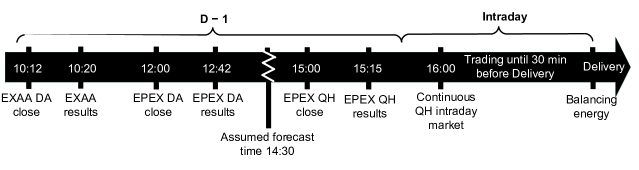
Figure 1: Spot trading timeline and its connected trading venues. All mentioned deadlines are assuming usual circumstances with no delayed results, technical problems and a market clearing price determined in the first run of the underlying algorithm. Please note that the intraday lead time of 30 minutes applies for cross-grid trades and local trades within the same grid area are allowed until 5 minutes before delivery.

Germany offers a wide variety of possible trading venues for market participants. Other countries usually exhibit a day-ahead spot exchange and continuous intraday trading platforms. These are also to be found for the four German grid areas, but besides them, there are two other auctions, as depicted in Figure 1. Spot trading ideally starts with the EXAA (Energy Exchange Austria) at 10:12am for final bid submission. Only 8 minutes later, the EXAA publishes the first day-ahead exchange traded quotation for the German delivery area. Although an Austrian exchange, EXAA results can easily be delivered into German market areas. However, we must acknowledge that this situation could be of temporary character with ongoing talks about splitting the German-Austrian bidding zone. As a result, EXAA volumes might only be transferred with explicitly sold cross-border capacities or are implicitly regarded by exchange auctions. One feature only available with EXAA is post-trading. The exchange platform allows for a second bidding round with known prices to market a surplus on either the buy or sell side. EXAA trading only occurs on non-holiday weekdays. All weekend or holiday prices are determined in advance on the last weekday before the holiday or weekend. Therefore, we already have a QH indication for delivery date Sunday on Friday, for instance. The next and

Exchange	traded volume [TWh]
	2015	2016	2017
EPEX DA auction	264	235	233
EXAA DA auction	8.2	8.0	5.4
EPEX QH auction	3.9	4.6	5.2
EPEX QH ID	3.9	3.6	4.9

Table 1: Yearly volumes of hourly and quarter-hourly German spot exchanges. All intraday figures only entail data on Germany, while the day-ahead auction includes Austria and Luxembourg.

presumably most important trading opportunity is provided by the German EPEX day-ahead (DA) auction. A single bidding round with results available at 12:42am marks the primarily traded market quotation in the day-ahead market. At the time of writing, the term ’EPEX day-ahead’ correctly specifies the German hourly day-ahead exchange. Still, the other exchanges, EXAA and Nord Pool Spot, are expanding their activities to the German day-ahead market. It is planned to unbundle the pricing algorithm from EPEX such that three independent exchanges offer access to the price that is hereinafter referred to as ’EPEX day-ahead’. We stick to that notation to be in line with other literature and due to the fact that these changes are planned but have not been implemented yet.
     Due to rising renewables infeed and the necessity to balance quarter-hourly deviations, EPEX launched a second auction for quarter-hours in December 2014. Strictly chronologically speaking it takes place day-ahead, nevertheless it is referred to as an intraday call auction because the day-ahead market window ends at d-1, 14:30pm for grid operators, as depicted by the white lines in Figure 1. While all prior marketplaces allow entering a single round of bids determining the price level in a closed-form auction, our last trading opportunity, the EPEX intraday market, is a continuous one that is tradable up to 30 minutes before delivery. This lead time was changed per July 2015 from 45 to 30 minutes. We will consider the volume weighted average price (VWAP) of all transactions for the specific delivery quarter-hour since continuous trading activities are difficult to quantify otherwise. Last but not least, all open positions will be settled by the grid operators in the course of balancing energy at the grid area independent imbalance tariff (reBAP). Since it is strictly forbidden by regulators to enter imbalance positions intentionally, this market is not a trading alternative and is just mentioned for the sake of comparability.
     Table 1 hints at the relevance of the different exchanges. The allocation of volumes points towards the immense importance of the hourly EPEX DA auction. It outruns the QH trading venues by far. This phenomenon might be explained by their purposes. As a result of missing liquidity, market players are more likely trading residual positions in QH markets. The majority, i.e., the hourly demand and generation will be bid in the day-ahead exchange for which reason QH liquidity only accounts for 2% of the DA liquidity. Unfortunately, EXAA volumes are reported in an aggregated form without any separation into hourly or quarter-hourly amounts. Hence, the mentioned trading volumes only allow for a rough evaluation of importance. The low volumes suggest that the EPEX markets are more momentous when German spot trading is concerned. Whenever liquidity is limited, this could elicit high volatility and price spikes. To detect such occurrences, we have plotted the price series in Figure 2. Both the QH auction and the ongoing QH intraday trading can be highly volatile with prices under 0€/MWh or above 100€/MWh. While, in general, both time series appear to follow similar trends, the intraday equivalent seems to feature more spikes. However, this effect is not predominant. The overall picture reflects two resemblant price quotations.

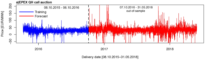
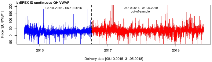
Figure 2: Price plot of the EPEX intraday QH auction and EPEX intraday continuous price regime separated into training and forecast sections. The blue partition marks the initial training and parameterization period that is consequently shifted with each iteration of the rolling estimation. The red line depicts the out-of-sample data that our prediction models try to forecast.

3 Forecast methodology

3.1 Data transformation and input parameters

The price plots reveal price spikes and the occurrence of negative prices. This is not a general problem but would usually require either an explicit modeling of spikes by means of a price spike component, a spike-robust model or a transformation to stabilize the variance of the time series (Uniejewski et al. (2018)). We have decided on the latter as we do not want to give up the feature selection abilities of our models discussed later. Once transformed, one can use a wider set of algorithms without taking greater care of price spikes. We firstly transform and then inverse the data such that the output of our models still appears in a realistic format. The transformation mainly supports the algorithms by providing a more stable variance but does not change any crucial information.
     A usual way to transform price series is the logarithm. While a simple logarithmic transformation works in many different scenarios, our time series with negative values necessitates a transformation method that can handle negative values. We stick to current literature findings to identify the best transformation for our needs. In a large empirical study, Uniejewski et al. (2018) report superior RMSE-related performance for a newly proposed transformation called ’mlog’, which we utilize for this paper. The authors especially propose the transformation for the spike sensitive measure RMSE (root-mean-square-error) which makes sense to apply to highly volatile time series such as our intraday one. The mlog transformation showed constant results across all markets, which is why we decided to use it for our time series and markets. Before its actual processing, the data requires normalization. Hence, the original time series $x_{qh,t}$ is adjusted to $z_{qh,t}=\frac{1}{MAD}(x_{qh,t}-median)$ in which MAD describes the median absolute deviation (MAD). Both MAD and median are calculated for $x_{qh,t}$ over the entire period. We purposely introduce a neutral time series notation $x_{qh,t}$ since the transformation procedure is not only executed on prices but on also other external factors like load or wind. Once the data is normalized, its transformation $y_{qh,t}$ is given by (taken from Uniejewski et al. (2018))

$$y_{qh,t}=sgn(z_{qh,t})\left[\mathrm{log}(\left|z_{qh,t}\right|+\frac{1}{c})+\mathrm{log}(c)\right],$$ (1)

and its inverse function

$$z_{qh,t}=sgn(y_{qh,t})\left[e^{\left|z_{qh,t}\right|-log(c)}-\frac{1}{c}\right],$$ (2)

with $c=\frac{1}{3}$. This parameter was likewise used by Uniejewski et al. (2018) and yielded good results across several markets.
     The time series is a quarter-hourly one which renders a slight transformation necessary. Daylight saving time causes one duplicate hour as well as a missing value. We follow Weron (2007) and average the duplicative hour. Its omitted equivalent is calculated using multiple imputations as presented in Buuren & Groothuis-Oudshoorn (2011) so that every day in the empirical test consists of 96 QHs. We also apply this approach to all other gaps in the time series. Apart from that, no more pre-processing is carried out. We neglect all outlier effects in our estimation scenario and leave extreme values untouched. Our empirical sample ranges from 08.10.2015 to 31.05.2018. Instructions on how to obtain the different data series are provided in Table 2. A solely autoregressive approach is not desirable as many papers suggest the influence that external factors have.

Figure 3: Averaged photovoltaics (PV) production forecast for Germany based on the publicly available TSO PV forecast. Please note that we have considered our entire time series from 01.10.2015 to 31.05.2018 and averaged across all 24 delivery hours in order to analyze any day and night effects.

We aim to keep the model simple and easily reproducible and only consider the most common publicly available external parameters like the quarter-hourly ENTSO-E load forecast (e.g. used in Kiesel & Paraschiv (2017)) or wind power reported by the EEX transparency platform (see Pape et al. (2016); Aïd et al. (2016); Garnier & Madlener (2015) for models that include wind infeed). The two input factors are fundamentally driven and might feature ramping effects. For instance, morning times when industrial shifts begin and people are waking up cause the grid load to quickly increase, whereas its level is more likely to be stable around noon. We embrace these effects for wind power production and load by regarding not only the load or wind infeed forecast for a specific hour but also the forecast from one hour previous. Strong differences between the two values might indicate ramping effects and can contain valuable information for our prediction model. Connected to these inputs is the concern over hourly data. Some prices and the wind data are present in hourly formats only. They are transformed rather modestly by assuming the hourly values for every quarter-hour without any further processing. Since we do not know anything about the quarter-hourly allocations, this seems to be the most unbiased way to capture these effects. As for wind, one might also find quarter-hourly forecasts by professional providers. We have deliberately chosen the hourly TSO data to ensure high reproducibility, but need to concede that designated vendor data increases forecast accuracy since it provides more accurate QH weather data.
     Speaking of weather data, one must not forget the other crucial component of the German fuel mix: Photovoltaics (PV) generation. A clear sign of its importance is that even the exchange itself mentions PV infeed as one of the major reasons for the introduction of the QH auction in 2013 (see EPEX (2013) for the press release). Märkle-Huß et al. (2018) support this assessment of importance by stating that QH trading is mostly driven by PV ramp-ups or -downs, i.e., times when PV production quickly increases or decreases. However, a forecaster needs to be careful with PV data. During the night, the time series features a constant zero due to no production which might cause problems with prediction models. Figure 3 illustrates how this effect is allocated over an entire day. The averaged PV production only starts to remarkably differ from zero in a time frame between hours 8 and 19. We have made the expert decision to add PV production data to all QH prediction models from quarter-hours 29 to 76 and ignore PV entirely in case of all other quarter-hours. We also want to capture ramping effects as in wind and load forecasts and consider the official TSO PV infeed forecast for the relevant hour together with its equivalent prediction one period before. Hence, our prediction approach accounts for ramp-ups or ramp-downs in PV production.
     Figure 1 is not strictly limited to quarter-hourly markets, but if we do so, three trading opportunities remain: the EPEX QH auction, continuous intraday trading and the EXAA auction which publishes results at 10:20am a day ahead. Therefore, the first quarter-hourly price information is delivered by EXAA prices. Its information might be incorporated into a forecasting scheme for the EPEX markets (see Ziel (2017) for this thought).

Determinant	Unit/granularity	Description	Data source	Transformation
EPEX day-ahead auction price	EUR/MWh, hourly	Market clearing price of the EPEX day-ahead auction, physical delivery into German or Austrian grid possible	European Power Exchange (EPEX), https://www.epexspot.com/en/	mlog, hourly value for all QHs
EPEX intraday auction price	EUR/MWh, quarter-hourly	Market clearing price of the EPEX intraday auction, physical delivery into German grid	European Power Exchange (EPEX), https://www.epexspot.com/en/	mlog
EPEX intraday VWAP	EUR/MWh, quarter-hourly	Volume weighted average of all transactions for specific QH, physical delivery into German grid	European Power Exchange (EPEX), https://www.epexspot.com/en/	mlog
EXAA day-ahead auction price	EUR/MWh, quarter-hourly	Market clearing price of the EXAA day-ahead auction, physical delivery into German and Austrian grid possible	Energy Exchange Austria (EXAA), http://www.exaa.at/en	mlog
ENTSO-E load forecast	MW, quarter-hourly	Vertical system load for bidding zone Germany/Austria, published around 10:00 d-1	European Network of Transmission System Operators (ENTSO-E), https://transparency.entsoe.eu/	mlog
TSO PV forecast	MW, hourly	Photovoltaics infeed forecast for Germany published by transmission system operators (TSO) at 8:00 d-1	European Energy Exchange (EEX), https://www.eex-transparency.com/	mlog, hourly value for all QHs
TSO wind forecast	MW, hourly	Wind infeed forecast for Germany published by transmission system operators (TSO) at 8:00 d-1	European Energy Exchange (EEX), https://www.eex-transparency.com/	mlog, hourly value for all QHs

Table 2: Overview of applied explanatory variables, their characteristics and how to obtain them for the sake of reproducibility.

Volume analysis has shown the importance of EPEX hourly auction prices. Around noon, these prices mark the benchmark for any spot trading activities. They provide an essential price indication for day-ahead trading. Possible impacts on this market are expected to have a partial influence on the intraday market as well.
     All external determinants and their data sources are summarized in Table 2. The calculations are made separately for every quarter-hour of the day. Such a method shrinks the size of all matrices in the calculation by 96 and reduces the computational effort immensely. On the other hand, quarter-hourly interdependencies evoked by ramping costs or similar load events are lost. Traditional thermal power plants have boundaries like start-up times. These might cause one quarter-hour to be profoundly affected by the preceding one. A principal component analysis (PCA) acknowledges these effects in

$$y_{h,t-1}\backsim\mathbf{\mathbf{\Lambda_{\mathrm{l,t}}}F_{\mathrm{l,t}}},$$ (3)

where $\mathbf{\Lambda_{l,t}}$ are the load factors and $\mathbf{F_{l,t}}$ the principal components of all 96 prices of today’s EXAA results, today’s EPEX day-ahead result and yesterday’s lagged prices of the market to be predicted. The components shall comprise all daily price information and are determined using all 96 quarter-hours. Please note that $l=1,...,96$ because 96 quarter-hours yield 96 components. We run the PCA over the EXAA and EPEX day-ahead prices since they are already available around 10:21 and 12:42 the day ahead and might give a good indication of the most current price interdependencies. In case of EPEX intraday continuous forecasts, we add a PCA on EPEX QH prices based on the same argument and data availability. In addition, a forth PCA on lagged prices tries to capture intraday dependencies in the markets we aim to predict. As with conventional PCA, the first few factors comprise sufficient information to be included. In our case, three components are utilized.
     While the ENTSO-E load forecast itself is already expected to contain a good portion of price information, its connected historical time series could deliver additional hints. Suppose that a specific load profile determines the shape of quarter-hourly demand. If we can identify days with a similar load curve, their observable prices provide valuable input for our forecasts. This idea was used in a comparable pre-filtering set-up by Maciejowska et al. (2016), one of the winning teams in a price forecasting challenge. We will likewise exploit this thought and aim to locate a similar load day from which to extract prices. The identified price will serve as another input feature. We aim to extract a vector out of our feature matrix that best approximates the day to be predicted with regards to its Euclidean distance. In other words, the Euclidean distance between the current day and all historical load observations is measured, and the minimum is determined. Once found, the prices of the most similar load scenario are plugged into the model assuming that they inherit crucial information about upcoming price developments.
     Regarding timing, we do not use any updated forecast data, i.e., intraday predictions are made at the same point in time that the QH auction prices are being estimated even though their computation is not restricted to fixed auction times. This is essential because we want to derive a coinstantaneous trading decision from the predictions, i.e., enter positions in both markets at the same time. However, it leads to a situation in which we use the most current data only for the QH auction. It is a trade-off for the sake of publicly available data and simultaneous applications of both forecasts to capture economic benefits.

3.2 Prediction model

The aim is to predict both the EPEX quarter-hourly intraday auction and the intraday continuous market price of the next day. An equivalent model is utilized for both markets which is why the following notations have a general character and are not restricted to one of the exchanges. Our deliberations start with a plain benchmark model, denoted as Naive_EXAA in the rest of this paper. Whilst in other market regimes the best naive guess is provided by yesterday’s price, the German market offers an idiosyncrasy in the form of the EXAA auction and its first indication for later auctions and continuous trading to follow. We exploit the EXAA results and expect them to be the best estimator for the other markets such that $\hat{y}_{qh,t}=y_{\mathrm{EXAA},qh,t}$. This model shall serve as an accuracy baseline for the other forecast approaches.
     Linear concepts tend to show convincing results in energy forecasting (see Maciejowska & Nowotarski (2016) for an example), which is why this paper sets the technical focus on them. Of course we could have used other predictors, like non-linear ones, but have decided to thoroughly introduce the overall model architecture instead of applying a wider set of models. For more information on other common forecasting approaches and their accuracy one might refer to Gürtler & Paulsen (2018). With reference to the described input factors, we introduce two general regression approaches that serve as a basis for all upcoming models. Our first input set, denoted by the prefix Expert_, takes expert decisions on weekly dummies and lags and is described in the following simplified form exemplarily for $y_{qh,t}$= EPEX quarter-hourly auction quotation

$$y_{qh,t} =\beta_{qh,0}+\sum_{\begin{subarray}{c}j\in\{1,2,7\}\\ i=(1,...,3)\end{subarray}}\underbrace{\beta_{qh,i}y_{qh,t-j}}_{\mathrm{\textrm{AR-terms}}}+\underbrace{\beta_{qh,4}\mathrm{\phi_{\mathit{1,qh,t}}}}_{\mathrm{\textrm{EEX wind}}}$$ (4)

$$+\underbrace{\beta_{qh,5}\mathrm{\phi_{\mathit{2,qh-1,t}}}}_{\mathrm{\textrm{EEX wind}lag}}+\mathbbm{1}_{(29,...,76)}(qh)\underbrace{(\beta_{qh,6}\mathrm{\phi_{\mathit{3,qh,t}}}}_{\mathrm{\textrm{EEX PV}}}+\underbrace{\beta_{qh,7}\mathrm{\phi_{\mathit{4,qh-1,t}}})}_{\mathrm{\textrm{EEX PV lag}}}$$

$$+\sum_{\begin{subarray}{c}k\in\{0,1,2,7\}\\ i=(1,...,4)\end{subarray}}\underbrace{\beta_{qh,7+i}y_{\mathrm{DA},qh,t-k}}_{\mathrm{\textrm{EPEX DA lags}}}+\sum_{\begin{subarray}{c}k\in\{0,1,2,7\}\\ i=(1,...,4)\end{subarray}}\underbrace{\beta_{qh,11+i}y_{\mathrm{EXAA},qh,t-k}}_{\mathrm{\textrm{EXAA QH lags}}}$$

$$+\underbrace{\beta_{qh,16}y_{\min,t-1}+\beta_{qh,17}y_{\textrm{max},t-1}}_{\mathrm{\textrm{non-linear\,effects}}}+\underbrace{\beta_{qh,18}\mathrm{\phi_{\mathit{5,qh,t}}}}_{\mathrm{\textrm{ENTSO load}}}+\underbrace{\beta_{qh,19}\mathrm{\phi_{\mathit{6,qh-1,t}}}}_{\mathrm{\textrm{ENTSO load lag}}}$$

$$+\sum_{\begin{subarray}{c}l=(1,...,3)\\ i=(1,...,3)\end{subarray}}\underbrace{\beta_{qh,19+i}\textrm{PC}\textrm{A}_{\mathrm{EXAA,}l}}_{\mathrm{\textrm{daily PCA factors}}}+\sum_{\begin{subarray}{c}l=(1,...,3)\\ i=(1,...,3)\end{subarray}}\underbrace{\beta_{qh,22+i}\textrm{PC}\textrm{A}_{\mathrm{EPEX\,DA,}l}}_{\mathrm{\textrm{daily PCA factors}}}$$

$$+\sum_{\begin{subarray}{c}l=(1,...,3)\\ i=(1,...,3)\end{subarray}}\underbrace{\beta_{qh,25+i}\textrm{PC}\textrm{A}_{\mathrm{EPEX\,QH,}l}}_{\mathrm{\textrm{daily PCA factors}}}+\sum_{\begin{subarray}{c}m=\{1,6,7\}\\ i=(1,...,3)\end{subarray}}\underbrace{\beta_{qh,29+i}D_{m}}_{\mathrm{\textrm{daily dummies}}}$$

$$+\underbrace{\beta_{qh,30}\mathrm{y_{similiar\mathit{,qh,t}}}}_{\mathrm{\textrm{similar load day}}}+\varepsilon_{qh,t},$$

with $y_{qh,t-k}$ being the mlog prices of the identical quarter-hour one, two and seven days ago and $y_{EXAA,qh}$, $y_{DA,qh}$ its equivalent lags for the EXAA and EPEX day-ahead market. Obviously, the AR-term changes with the market to be predicted. The terms $y_{\min,t-1}$ and $y_{\textrm{max},t-1}$ refer to yesterday’s minimum and maximum mlog price and are supposed to reflect the non-linear interdependency between the daily price regimes, while $\phi_{\mathit{1,qh,t}},...,\phi_{\mathit{6,qh,t}}$ are the wind, PV and load forecasts for the respective delivery day and its lagged values. We use the previous hours’ lagged values to capture ramp-up effects of our fundamental variables. The notation $y_{\mathrm{similar},qh,t}$ describes prices of the minimum Euclidean distance load scenario as mentioned in the previous sub-chapter, i.e., prices of a day that feature a similar load profile with regards to the Euclidean distance between the current load forecast and all historical ones.
     The term $D_{k}$ is a dummy variable (i.e., taking a value of 1 in case of occurrence) to capture the intra-week term structure with $m=1,6,7$ for Monday, Saturday and Sunday. Weekly seasonality is a crucial factor for spot electricity prices like the ones present (see also Weron & Misiorek (2008) for an example on three weekly dummies). Saturday and Sunday differ from the rest of the week due to their weekend characteristics, with less traders being active and lower load and energy production levels. Our markets might be traded day-ahead, so even Monday could differ from typical weekdays due to the fact that quantities were traded on a Sunday. The argument certainly holds true for the day-ahead traded QH auction and intraday continuous markets are at least partially traded one day in advance. We therefore apply the set-up on both markets. The notation $\textrm{PC}\textrm{A}_{\mathrm{EXAA},l}$ defines the $l-\mathrm{th}$ principal component of the EXAA QH prices. Besides EXAA, we include PCA’s for EPEX QH and EPEX day-ahead prices. The error term $\varepsilon_{h,t}$ is assumed to be independent and identically distributed (iid) with $\varepsilon_{h,t}\sim N(0,\sigma_{qh}^{2})$. In case of EPEX intraday continuous prices we slightly expand Eq. (4) by adding its relevant auto-regressive lags, the current EPEX QH auction price as well as a PCA on the intraday continuous prices. They are available before the continuous trading window starts so it makes sense to exploit them for forecasting models. Please note that our model in Eq. (4) is a multivariate one meaning that we have an independent estimation per quarter-hour or, in other words, 96 autarkic models.
Using expert decisions inevitably means subjectivity and leaves room for criticism. We include a second input set called Full_ that overcomes all concerns over possible bias. Instead of weekdays for Monday, Saturday and Sunday the full model implements dummies for every day of the week (such that $m=1,...,7)$ in equation (4). It also includes all 7 lags for every quarter-hourly price compared to the expert model only using lag 1,2 and 7. Lastly the full model replaces all PCA’s with 96 prices per quarter-hour for EXAA, EPEX QH, EPEX day-ahead and -in case of the intraday continuous prices to be predicted- for EPEX intraday. This expansion causes the model structure to be much more complex than before. The full model features 254 predictors in case of QH auction predictions and over 300 for intraday continuous forecasts. Such an expansive model might serve as a sensitivity check. If our expert decisions are correct, than the models shall result in similar accuracy.
     The $\beta_{qh,1,...,30}$ parameters in Eq. (4) are determined by the well-known ordinary least squares (OLS) optimization in our first model, leading to the estimator called LM hereinafter. One of the key points of this paper is an evaluation of the ideas in Ziel et al. (2015) and Ziel (2017). Does the EXAA price add accuracy gains in QH markets? We introduce a second model, LM_EXAA, with one slight difference to Eq. (4). All parameters remain unchanged for the prediction of both intraday and auction markets, but we add the EXAA quarter-hourly auction results as another explanatory variable. The sources above found evidence for accuracy gains once EXAA prices were included, which is why we expect them to enhance our models in a similar fashion.
     Another concern indirectly arises from Eq. (4). We use a large set of input factors where many features are assumed to be correlated. We apply a PCA but include a selection of lagged values which are again inputs for the PCA. Hence, high correlation in our predictors needs to be taken into account together with the fact that too many variables could cause overfitting. A second linear prediction model, denoted as EN, shall overcome this limitation. Introduced in Zou & Hastie (2005), elastic nets (EN) balance between linear and quadratic penalty factors or between lasso and ridge regression. Its great advantage is that it combines aspects out of the latter two algorithms, such that elastic nets can automatically remove unneeded variables entirely from the model while also being more robust to correlation than the lasso. We simplify the model in Eq. (4) to the regression form

$$y_{qh,t}=\sum_{j=1}^{p}\beta_{qh,t,j}x_{qh,t,j}+\varepsilon_{qh,t}.$$ (5)

The OLS optimization aims to minimize the residual sum of squares (RSS). The elastic net estimator expands this approach by adding a linear penalty factor $\lambda_{qh}\geq 0$ in

$$\hat{\mathbf{\mathbf{\mathrm{\boldsymbol{\beta}}}}}_{\mathbf{EN}}=\operatorname*{arg\,min}_{\mathbf{\boldsymbol{\beta}}_{\mathit{\mathbf{qh}}}}\left\{RSS+\underbrace{\lambda_{qh}\left(\frac{1-\alpha}{2}\sum_{j=1}^{p}\beta_{qh,j}^{2}+\alpha\sum_{j=1}^{p}\left|\beta_{qh,j}\right|\right)}_{\mathrm{\textrm{Penalty Term}}}\right\},$$ (6)

$$\mathrm{where\;RSS}=\sum_{t=1}^{T}(y_{qh,t}-\sum_{j=1}^{p}\beta_{qh,j}x_{qh,t,j})^{2}.$$

In case of $\lambda_{qh}=0$ we obtain the same results as for the OLS-based LM model. The other extreme case $\lambda_{qh}\rightarrow\infty$ causes all variables to be shrunken to zero, i.e., removed from the model or tending to zero depending on the weighting between lasso and ridge regression. The allocation between ridge and lasso is described by the parameter $\alpha\text{$\in$}\text{[0,1]}.$ We follow the findings of an empirical study in Uniejewski et al. (2016) and set $\alpha=0.5$ as subjective expert decision, that is justified by good predictive performance reported in the literature. The optimization itself might be seen as a trade-off between minimizing the RSS and simplifying the model structure. Besides, an elastic net is a form of variable selection due to its ability to cancel out entire input factors. A regularization method such as the elastic net urgently necessitates normalization and standardization to yield valid results. The penalty term works by both scale and magnitude of the variables while we desire a sparse solution based solely on the individual magnitude. However, the topic of standardization is of no concern in our context since the mlog transformation explicitly regards this aspect. Please note that in case of standardization there is no necessity for an intercept anymore which is why there is none in Eq. (4).
     Equation (6) leaves an optimization problem to be solved. We compute a solution using R’s glmnet package by Friedman et al. (2010). The optimization computation requires a measure to be minimized, and in our case that is the mean squared error (MSE). Based on a user-specified number of 1,000 different steps for $\lambda_{qh}$, glmnet automatically creates an exponential grid starting from $\lambda=0.001$ to a data-derived maximum per each quarter-hour and determines the best value based on a 10-fold cross-validation. Despite being more time intensive than a simple optimization, our cross-validation set-up provides generalization with regards to the selected $\lambda_{qh}$. Just like the previous OLS model, a second predictor EN_EXAA comprises the quarter-hourly EXAA quotations of the delivery date.

4 Back-test results

4.1 Point forecast performance

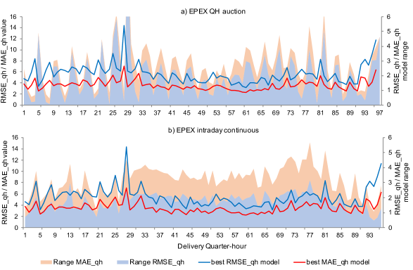
Figure 4: Quarter-hourly model fit metrics MAE_qh and RMSE_qh and range of MAE_qh and RMSE_qh between best and worst model. The plot is limited to the best performing model per market, in case of the QH auction that is Full_EN and for the intraday continuous market it is Expert_EN. Please note that we have excluded Full_LM and Full_LM_EXAA from the plot due to its unreasonably high error metrics.

Before turning the attention to economic gains stemming from accurate forecasts, the predictive performance of our models in question requires discussion. Rolling estimations assure realistic simulation results. Hence, every model is iteratively fitted and predicts on new data, while afterward the entire data matrix is shifted by 96 quarter-hours. This modus operandi ensures that all predictions are made on out-of-sample data and reflects realistic behavior in practical applications. We train our model with nearly one year of data so that a period spanning from 08.10.2015 to 06.10.2016 is utilized for the initial training. From 07.10.2016 to 31.05.2017 all values are predicted in an out-of-sample manner such that we have 57,714 individually estimated quarter-hours to be evaluated in all upcoming tests. Given this vast amount of data, we believe the test results to be sound.
     We report two commonly used measures, the root-mean-square-error (RMSE) and mean-absolute-error (MAE), given by

$$\mathrm{RMSE}=\sqrt{\frac{1}{96T}\sum_{t=1}^{T}\sum_{qh=1}^{96}(y_{qh,t}-\hat{y}_{qh,t})^{2},}$$ (7)

$$\mathrm{MAE}=\frac{1}{96T}\sum_{t=1}^{T}\sum_{qh=1}^{96}(\left|y_{qh,t}-\hat{y}_{qh,t}\right|),$$ (8)

where $T$ describes the number of days, $y_{qh,t}$ the observed prices and $\hat{y}_{qh,t}$ its predicted counterpart. All results are reported in Table 3.

Table 3: Error measures root-mean-square-error (RMSE) and mean-absolute-error (MAE) for applied forecast models.

They suggest that the quarter-hourly auction indeed benefits from forecasts based on external factors since the difference between the benchmark model and the best performing EN estimator is more than 20% in the RMSE case. The LM model is better than the naive benchmark, and the elastic net approach tops that by roughly the same accuracy gain that separated the LM and the naive model for both RMSE and MAE. Given our range of auction data, advanced linear modeling seems to add a crucial portion of performance. Interestingly, our choice of expert decision was not entirely correct since the full models feature lower MAE and RMSE values. However, this is not the case with LM models. As expected, they cannot handle the massive set of inputs and feature the highest RMSE and MAE results when enriched with all inputs.
     At the same time, the EXAA as a model input leaves the impression of minor importance. EXAA-enriched EN models outperform their rivals by around 3% for the QH auction if we consider the RMSE. Still, this effect has been expected to be higher and is only limited to the elastic net that can handle numerous input factors. The common OLS-based LM model rather seems to suffer from more inputs. The EXAA provides a quarter-hourly quotation for the same delivery date but only slightly improves the models. This could either be caused by the time lag from result publication at 10am to EPEX bidding at 3pm or the different intraday characteristics respectively. Indeed, one might argue that 5 or more hours could lead to new wind forecasts and changed QH bids. Another thought is connected to the hourly day-ahead auction. Presumably, market participants wait for the most important German spot auction until they actively trade-out their quarter-hourly shapes. Thus, the EXAA auction could be characterized by different market players and changing bidding behavior. However, these thoughts require quantitative backing in further research.
     The picture changes with the EPEX continuous intraday market. The performance is almost two times worse than QH auction results in case of EN predictions. Both MAE and RMSE are considerably higher for intraday estimations. An initial guess might be that this observation is associated with even more substantial intra-model deviations. However, the results suggest a different outcome. The linear models only slightly increase the performance in comparison with the usage of plain EXAA prices as a prediction model input. Whereas elastic net outperforms the OLS-based predictor in QH auctions, its performance gain is only marginal in the intraday regime. Our empirical test suggests the same results for the question of EXAA influences on performance. An accuracy increase of around 1% does not support the argument of strong EXAA implications in continuous intraday markets. The market itself features an entirely different pricing regime which tends to either be more complicated in prediction or influenced by other parameters. Besides that, the timing aspect also matters. All intraday forecasts exploit the same fundamental data that was used for the QH auction. Updated wind or load data could boost accuracy. In terms of input factors our expert models are comparable to the full models with one exception; while the linear model was already struggling for QH auction data, the intraday continuous trading proves it to be unsuitable for large numbers of regressors. Its error measures clearly indicate a model issue and unreasonable point forecasts.
     Figure 4 provides a graphical representation of the model fit. Please note that we change eq. (7) and (8) to a quarter-hourly representation by adding the identically named suffix. It shows the quarter-hourly term structure of the best performing MAE_qh and RMSE_qh model as well as the range between the best and worst performing model. It appears that each hour’s last quarter-hour is harder to estimate with higher RMSE_qh and MAE_qh results. This results in a characteristic zig-zag pattern in both markets. Besides, the transition phase from off-peak to peak between hour 7 and 8 and hour 20 to 21 is a common time of higher uncertainty. Additional plants are ramped up to cover tradeable peak profile demands. These effects are observable in higher error measures in Figure 4. The overall QH auction’s error range is constant besides the last QH and off-peak/peak changes but the intraday continuous plot reveals higher model deviations for the entire peak time. So this market appears to be more difficult to predict in peak hours.

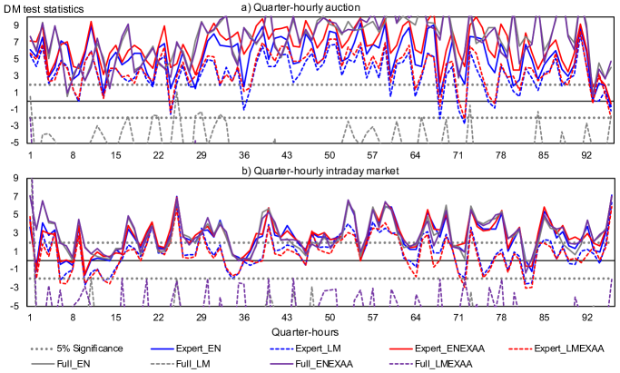
Figure 5: Quarter-hourly Diebold-Mariano test statistics carried out under the absolute loss function and with loss series lagged four times determined by an AR(p) process.

A more advanced test measure is delivered by Diebold & Mariano (1995) in the eponymous Diebold-Mariano (DM) test statistics. It has proven to be a profound measure with energy pricing applications in Nowotarski et al. (2014) and Bordignon et al. (2013) and aims at investigating the outperformance of one model forecast over the other. The test input parameters are given by the loss differential series $\Omega_{qh,t}^{m1,m2}$ of the absolute error of models $m_{1},m_{2}$ such that

$$\Omega_{qh,t}^{m1,m2}=\left|y_{qh,t}^{m1}-\hat{y}_{qh,t}^{m1}\right|^{p}-\left|y_{qh,t}^{m2}-\hat{y}_{qh,t}^{m2}\right|^{p}.$$ (9)

Depending on the choice of $p$, the quadratic loss or the absolute loss is applied. Our tests did not reveal any considerable difference in the test results for either $p=1$ or $p=2$ which is why we stick to the former. An essential prerequisite of the test is non-covariance stationarity in errors as discussed in Diebold (2015). Daily test statistics might contradict this postulation since all of the quarter-hours are driven by the same daily fundamental drivers as proposed by Nowotarski et al. (2016). Our univariate approach eludes this matter by its finer resolution. Another concern arises from autoregressive structures. Since we include at least three lags, the quarter-hours and their connected prices must be correlated. This issue is dealt with by using lagged errors for Eq. (9). We inspect the partial auto-correlation function and fit an AR(p) process to the intraday and QH auction time series (see Ziel et al. (2015) for the idea of fitting an AR(p) process to tackle correlation in the DM test) to identify the most suitable lag order. In our case, an error series lagged four times appears to be statistically sound. The test itself is performed at the 5% significance level and reflects consistent outperformance against the naive benchmark model.

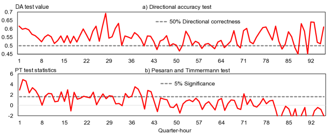
Figure 6: Directional forecast evaluations based on a) Directional Accuracy statistics and b) the Pesaran and Timmermann test. The term ’directional’ describes whether the set of forecasts for the EPEX QH auction and ID continuous market is capable of identifying the high price and low price trading venue.

Figure 5 provides a graphical representation of the DM test results. The higher the test statistics for every quarter-hour are, the better the model performs in comparison with the benchmark model. Furthermore, all values under or above the dotted gray line depict significant overperfomance or underperformance of the respective model. Bearing this in mind, Figure 5 supports the conclusion drawn from the RMSE scores. Nearly all linear models with expert choices tend to improve forecast accuracy for the QH auction with the EXAA-enriched ones better than non-EXAA predictions, and EN estimates slightly more precise than its OLS opponent. The LM models show significantly negative performance compared to the benchmark, which again highlights their inability to deal with larger amounts of regressors. All models seem to suffer in the same period around QH 36. We can acknowledge that EXAA slightly matters for the QH auction market based on our empirical study since DM statistics are a bit higher for these models. Still, the effect is very limited. The differences among the continuous intraday models are reasonably low. Very few QHs show tendencies of statistical excess performance, and even in these scenarios, it is difficult to favor a specific model. The majority of observations are to be found in the range below 5% significance meaning neither LM, EN or EXAA enrichment leads to fewer errors compared to our benchmark. This outcome was unanticipated but might again be due to the time lag between estimations and continuous intraday trading activities.

4.2 Economic effects of accurate forecasts

4.2.1 Directional forecast portfolio approach

A single point forecast has limited value if considered separately without a translation into a trading decision. We will introduce two different approaches that shall use the forecasts as an input and transform these into a QH deal. Buying and selling are regarded in different portfolios to reflect possible gains for net buyers and sellers. Based on these thoughts, we firstly utilize both predictions in a simplified binary scheme. Companies need to buy or sell their residual quarter-hourly spot profile on spot exchanges and shall do so based on the simple rule of buying in the cheaper market (low market) and selling in the more expensive one (high market). Hence, a sell position is entered into the market with higher predicted prices, denoted as Base_Sell, while the Base_Buy portfolio buys in the lower projected market. Since the previous sub-chapter reflected an apparent tendency towards the EN predictors being the best, we consider EN and EN_EXAA for our analysis and introduce additional portfolios, Base_{Sell_EXAA}and Base_{Buy_EXAA}. These will explicitly include the information provided by EXAA prices just as in the EN and LM forecast models.
     The above idea narrows the deal determination down to a directional forecast based on the high and low market. Therefore, we want to elaborate the directional accuracy of our approach. The common measure (i.e., used in Moosa & Vaz (2015)) Directional Accuracy (DAcc) delivers the first hint of the binary accuracy of our forecasts in a directional setting and is defined in a low market/high market application as

$$DAcc=\frac{1}{n}\sum_{i=1}^{n}d_{qh,t},$$ (10)

with the connected hit series

$$d_{qh,t}=\begin{cases}1,&\mathrm{if}\,(\hat{y}_{qh,t}^{m1}>\hat{y}_{qh,t}^{m2})\land(y_{qh,t}^{m1}>y_{qh,t}^{m2})\\ 0,&\mathrm{if}\,(\hat{y}_{qh,t}^{m1}<\hat{y}_{qh,t}^{m2})\land(y_{qh,t}^{m1}>y_{qh,t}^{m2}).\end{cases}$$ (11)

Intuitively speaking, Eq. (11) assigns a value of 1 every time the higher or lower market is correctly predicted. The representation is kept general, but in our given case the model indices $m1,$ $m2$ denote either the EPEX QH auction or the QH intraday market. Once we know whether the prediction of the higher market is right or wrong, the DAcc measure in Eq. (10) reports the share of correct directional estimates. The second framework is provided by Pesaran & Timmermann (1992) and supposes independent directions of the observed and predicted realizations under the null hypothesis, i.e., that estimated directions do not add extra knowledge. Both metrics will be reported quarter-hourly to gain additional insights into the time structure accuracy of the predictions.

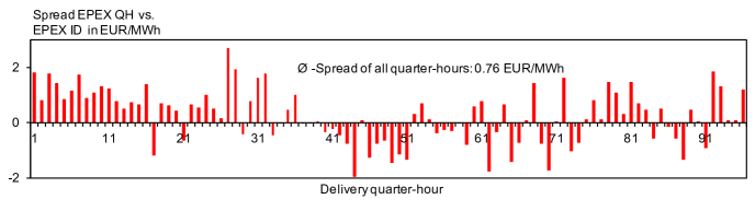
Figure 7: Quarter-hourly spreads of portfolio strategy Base_{Sell_EXAA}/Base_{Buy_EXAA}, i.e., sell in the predicted high market and buy in its lower equivalent. The markets under consideration are the continuous QH intraday market and the EPEX QH intraday call auction.

	Portfolio ID	Description	Price	Min Price	Max Price	Std.Dev	Sharpe- Ratio
Benchmark portfolios	NaiveEXAA	EXAA QH trading of residual volumes	34.95	-102.34	168.85	17.18	2.04
	NaiveAUQH	EPEX intraday QH auction trading of resuming position	34.66	-134.82	290.65	19.15	1.81
	NaiveIDQH	EPEX intraday QH VWAP trading of residual position	34.81	-241.83	329.81	20.27	1.72
	NaivereBAP	Settlement of residual position at reBAP price with grid operator	34.74	-2558.42	24455.05	147.54	0.24
	PerfectBuy	Full information benchmark portfolio, always buys in lower market	30.74	-241.83	166.42	19.40	1.58
	PerfectSell	Full information benchmark portfolio, always sells in lower market	38.73	-117.77	329.81	19.22	2.02
Forecast portfolios	BaseBuy	Buy in market with lowest predicted price using EN	34.38	-173.94	329.81	19.83	1.74
	BaseSell	Sell in market with highest predicted price using EN	35.09	-241.83	266.17	19.61	1.78
	BaseBuy_EXAA	Buy in market with lowest predicted price using ENEXAA	34.36*	-173.94	329.81	19.84	1.73
	BaseSell_EXAA	Sell in market with highest predicted price using ENEXAA	35.11**	-241.83	266.17	19.59	1.79
	MeanVarBuy	Mean-variance portfolio with lowest return, i.e., lowest price to pay using EN	34.71	-178.50	245.99	19.09	1.83
	MeanVarSell	Mean-variance portfolio with highest return, i.e., highest price to sell using EN	34.76	-173.89	213.02	18.62	1.87
	MeanVarBuy_EXAA	Mean-variance portfolio with lowest return, i.e., lowest price to pay using ENEXAA	34.72	-178.50	245.99	19.00	1.83
	MeanVarSell_EXAA	Mean-variance portfolio with highest return, i.e., highest price to sell using ENEXAA	34.76	-173.89	213.02	18.62	1.87

Table 4: Empirical test results of different portfolio strategies in the case study period from 07.10.2017 - 31.05.2018. The prices are not volume weighted nor adjusted in any way and reflect the price one would buy or sell at given the selected portfolio strategy. Naive prices denote the simple average of the respective price series. Both the lowest buy price (*) and the highest sell price (**) are marked for convenience.

Figure 6 summarizes the findings in a combined way. The upper plot shows that using the individual forecasts to estimate the cheaper or more expensive exchange leads to more than 50% correctness in most cases. In general, this is a promising finding since once we have a higher correctness rate than 50%, there is a possibility to observe economic benefits. However, this postulation only holds true if the losses of an incorrect prediction and the gains of a correct one are equally distributed such that the cost of making a wrong prediction is nearly equal to the benefit of being correct. On the other hand, we see a decline in directional accuracy in the peak QHs ranging roughly from quarter-hour 36 to 70. Our estimations seem to be more accurate in off-peak regimes given the dataset. This message is supported by the second metrics depicted in the lower part of Figure 6. The Pesaran and Timmermann (PT) test statistics exhibit an off-peak/peak pattern. The actual test score is contradictory to the measure mentioned before. The majority of quarter-hours do not pass the test, meaning that we found evidence that the correct direction and its predicted equivalent are less independent than desired. This outcome was unforeseen considering the results of the Directional Accuracy test. To conclude, the tests suggest a promising rate of correctness but do not allow us to reject the null hypothesis of autonomous directional errors. The forecast quality might be biased. Still, we have to acknowledge that we only want to investigate the economic value of our point forecasts and have translated them into a binary framework. So, they could be distorted since the basis is not a designated directional estimation.

4.2.2 Mean-variance portfolio selection

A different portfolio composition technique is given by mean-variance portfolio selection. Initially introduced in Markowitz (1952), its classical scope covers financial markets and the selection of stocks under expected return and variance. However, there are a few energy market applications of mean-variance concepts available (the interested reader might refer to a recent review of this topic in Calvo-Silvosa et al. (2017)). To apply such, the definition of return needs to be clarified. Financial markets assume a fixed asset position with payments of price movements leading to a return given by $r_{\mathrm{traditional},qh,t}=(y_{qh,t}/y_{qh,t-1})-1$. This notation makes sense for storable assets or long-term power contracts but does not apply to a spot market example. Long-term contracts, like futures, are usually settled daily in a margining process such that only the price difference is paid or received. The same holds true for a stock position. In spot markets, the daily position will most likely be different due to changing off-take or power plant generation. Hence, the resulting cash-flow is different. A consecutive two-day long position of 50MW will not just be settled at the price delta between day one and day two (as done with futures and daily margining), but a market participant has to pay 50 MW times the market price. Therefore, we will regard the price itself as the return leading to our notation $r_{qh,t}=y_{qh,t}$. Another difference is given by the differentiation into buy and sell portfolios. Once we value a high return (or in our notation a high clearing price) as desirable and optimize with regards to that, we will identify a sell portfolio because a market player obviously demands high prices and high returns. The buy portfolio is the inverse of the particular optimization result and yields lower returns or lower prices for net buyers in the market.
     The mean-variance theory incorporates expected returns and variance into an optimization framework. Individual assets numbered by $i=1,...,n$ are weighted by a factor $w_{i,qh,t}$ to compose a portfolio of assets. In our concrete case, the portfolio is restricted to two assets or the choice between the QH intraday auction and continuous intraday trading. Unlike financial applications, we do not include any risk-free benchmark assets. Using our prices as single time series returns in the Markowitz sense leads to a portfolio return in

$$r_{\mathrm{portfolio,\mathit{qh,t}}}=\sum_{i=1}^{2}w_{i,qh,t}y_{i,qh,t},$$ (12)

where $y_{i,qh,t}$ are the realized values for either the QH auction or the intraday market and $w_{i,qh,t}$ are the connected weights. Yet, Eq. (12) only provides insights into the historical return and does not comprise any future-oriented quantification. Markowitz optimizations require expected returns denoted as $E(r_{\mathrm{portfolio,\mathit{qh,t}}})$ which inevitably necessitates expected single $i$-th returns, i.e., $E(r_{i,qh,t})$$=E(y_{i,qh,t})=\mu_{i,qh,t}$. Instead of the traditional mean formulation, we want to approximate the expected return by means of our forecasts so that $\mu{}_{i,qh,t}\sim\hat{y}_{i,qh,t}.$ Pruning the notation to just a single weighting factor and taking into consideration the thoughts on expected return yields a more simple form such that

$$E(r_{\mathrm{portfolio,\mathit{qh,t}}})=\hat{y}_{1,qh,t}+w_{2,qh,t}(\hat{y}_{2,qh,t}-\hat{y}_{1,qh,t}).$$ (13)

The variance is determined by a simplifying relaxation. Instead of complex estimation schemes, we will apply the empirical variance $\sigma_{i,qh,t}^{2}$ of the individual exchange return series and assume it to be the best estimator in the calculation of the portfolio return in

$$\sigma_{\mathrm{portfolio},qh,t}^{2}=(w_{1,qh,t}^{2}\sigma_{1,qh,t}^{2})+(w_{2,qh,t}^{2}\sigma_{2,qh,t}^{2})+2w_{1,qh,t}w_{2,qh,t}\rho_{12,qh,t},$$ (14)

with $\rho_{12,qh,t}$ being the correlation of the returns. We simplify Eq. (14) to eliminate $w_{1,qh,t}$:

$$\sigma_{\mathrm{portfolio},qh,t}^{2}=\sigma_{1,qh,t}^{2}+2w_{2,qh,t}(\rho_{12,qh,t}-\sigma_{1,qh,t}^{2})$$ (15)

$$+(w_{2,qh,t}^{2})(\sigma_{1,qh,t}^{2}-2\rho_{12,qh,t}+\sigma_{2,qh,t}^{2}).$$

An important part of portfolio theory is the identification of all efficient portfolios under non-zero weights and a sum of weights equal to one. The latter postulation results in the assumption of perfectly divisible asset portions. We follow this traditional concept but must acknowledge that under real-life trading circumstances the exchange pre-defined minimum tick sizes condition small adjustments to the optimization results due to the fact that they are not tradable. We are also not interested in computing the entire set of efficient portfolios but want to find the one portfolio that exhibits the highest utility for the market participant. The utility function is defined as an optimization problem in (basic form taken from Calvo-Silvosa et al. (2017))

$$U_{qh,t} =\operatorname*{arg\,min}_{\mathit{w_{2,qh,t}}}E(r_{\mathrm{portfolio,\mathit{qh,t}}})-\frac{1}{2}\gamma\sigma_{\mathrm{portfolio},qh,t}^{2}$$ (16)

$$\mathrm{s.t.\;}\; w_{i,qh,t}\>\text{$\in$}\>[0,1],$$

in which $\gamma$ denotes a variable to specify the risk-aversion of the market participant. We follow the energy literature and set $\gamma=2$ which is regarded to be a slightly higher average risk appetite (Gökgöz & Atmaca (2012); Liu & Wu (2007)). Given the high variance of the intraday series an adjustment towards less risk aversion appears to be suitable. Otherwise, the optimization will mostly select the QH auction market. At the same time, the slight changes to the original equations in Eq. (13) and Eq. (15) yield only one weighting parameter $w_{2,qh,t}$ to be optimized. If we consider that possible solutions are restricted to be anything between zero or one, it becomes evident that we implicitly meet the requirement $\sum_{i=1}^{2}w_{i,qh,t}=1$. We use R’s standard optimization command optim to find a solution for Eq. (16). The optimization result yields two trading indications; if we value positive returns as desired to sell at high prices, the portfolio MeanVar_Sell is the important one whereas its counterpart MeanVar_Buy sets the focus on negative returns and lower prices for a net buyer. The same contentual separation counts for the EXAA-enriched equivalents MeanVar_{Sell_EXAA} and MeanVar_{Buy_EXAA} respectively.

4.2.3 Economic portfolio assessment

Now that we have determined different portfolio strategies with EXAA and non-EXAA variations, the last facet to assess is the economic gain or loss resulting from our underlying forecasts and portfolio strategies. For the sake of simplicity, we neglect all kinds of fees and trading charges as well as the price impacts possible bids might have. Hence, we assume sufficient market liquidity to absorb additional trading volumes. Last but not least, volume weighted average prices (VWAP) are only an approximation for continuous market prices. Apparently, a market participant does not have direct access to index quotations. Instead, regular trading activities could lead to average deal prices near the VWAP. Since the intraday trading activities are up to individual counterparts, with a detailed time series not being available, we apply the VWAP as a best guess. Based on these prices, we carry out a simple portfolio simulation and check the average portfolio price a market participant would pay or receive when following the portfolio strategy. The back-test ranges from 07.10.2016 to 31.05.2018 and is summarized in Table 4 together with a synopsis of all portfolio strategies. We use the original prices to get the most realistic results. The only adaptation we apply is the clock-change adjustment described under sub-section 3.1. We acknowledge that this causes a small bias but since it only accounts for two hours of each year we ignore the clock-change in the trading simulation. Besides the usual standard measures on time series resolution, we report a common portfolio management criterion called Sharpe-Ratio (adjusted from Calvo-Silvosa et al. (2017))

$$S=\frac{\frac{1}{96T}\sum_{t=1}^{T}\sum_{qh=1}^{96}(y_{\mathrm{strategy},qh,t})}{\sigma_{\mathrm{strategy}}},$$ (17)

where the numerator describes the average realized price of the respective portfolio strategy over all days and quarter-hours and $\sigma_{\mathrm{strategy}}$ the standard deviation of the realized prices of each strategy. The strategy prices $y_{\mathrm{strategy},qh,t}$ are individually determined per strategy, as previously described. In case of Base_Sell for instance, the strategy prices equal the market price of the higher predicted exchange. Please bear in mind that in its conventional form the Sharpe-Ratio applies the average excess return, but since we set the risk-free rate to be equal to zero, this step is not necessary, and the realized portfolio price is identical to the excess return.
     The naive portfolios only buy or sell in one market at the simple average of the time series and consequently yield lower sell and higher buy prices. There is no buy or sell separation with the naive prices while the forecast approaches imply a buy and sell market price. Consequently, our naive singular market strategies yield no spread benefits. We likewise report a perfect portfolio strategy under the assumption of complete market information. The results are highly unlikely to be achieved in a real-world scenario but represent the obtainable gains from fully accurate forecasts. However, we will not discuss the perfect portfolio in depth but focus our attention on achieved spreads compared to singular market activities as these depict current market participant behavior more than the postulation for complete ex-ante market knowledge. In general, the forecast portfolios perform well. Our results point towards an outperformance of high/low market interaction referred to as Base_Buy and Base_Sell and their EXAA-enriched equivalents.

In detail, market participants buy 0.70 - 0.74€/MWh cheaper and sell 0.74 - 0.78€/MWh higher compared to any other of the individual markets. Interestingly, the addition of EXAA prices yields higher spreads. While the EXAA-aided point forecasts become only a bit more accurate for the QH auction, the directional accuracy tends to improve. This finding seems contradictory at first, but might be the case since a directional forecast does not advance from a precise point prediction but solely from correct high/low market estimates.
     The Markowitz approach adds a considerably lower portion of economic gains. Its portfolio structure is a trade-off between the auction and continuous intraday prices. The realized portfolio price varies between the QH auction and its continuous equivalent. A possible explanation might be given by the Markowitz inputs. The optimization has to split between the highly volatile intraday continuous market and the more moderate QH auction. Most of the time, this results in a significant portion of QH auction prices due to risk aversion tendencies. Hence, if one considers the utility function in Eq. (16), a more risk averse portfolio is created. While the plain prices do not suggest larger benefits from following Markowitz-guided trading in comparison with the base strategies, the Sharpe-Ratio and standard deviation do. Both the Markowitz portfolio and the Sharpe-Ratio include a variance measure in their calculus. Therefore, it does not come as a surprise that the best Sharpe-Ratio results are provided by mean-variance portfolios. Still, we would have expected at least a small portion of economic benefit expressed in better spread levels. An explanation for the performance is the concern over correlation. Our choice of assets was predetermined, and we have not checked the correlation between the time series, but in financial markets, the co-movement among stocks contributes to a less balanced portfolio composition. The picture might change with less correlation between assets. However, the empirical results do not provide evidence for Markowitz approaches to perform better regarding higher spreads but construct a risk-minimizing portfolio. Therefore, we favor the simple base strategies that are grounded on a high/low market scenario and will purely focus on such in the detailed analysis.
     A simple t-test depicted in Table 5 is supposed to deliver further evidence on the statistical soundness of the identified excess performance. The p-values propose significant differences between our forecast-aided base portfolio prices and the intraday continuous time series. The QH auction result is less clear and shows signs of correlation with the non-EXAA base strategies. The result at least partially confirms our findings. Forecast applications translated into a simple buy/sell trading decision result in different portfolio price means compared to the underlying individual prices. There are tests available for the equality of Sharpe-Ratios. They use the portfolio prices as inputs and check for statistically sound differences among Sharpe-Ratios. We apply the classical pairwise test of Ledoit & Wolf (2008) and an expansion that considers joint effects of prices in a multiple Sharp-Ratio test in Leung & Wong (2008) and later for non-iid cases in Wright et al. (2014). Results are reported in Table 5. While the multiple test statistics clearly point towards independent Sharpe-Ratios, some of the pairwise test findings have to be rejected. However, this does not contradict our general statement of independent, considerable differences in prices when using forecasts since most of the combinations that appear to be correlated are using a slightly changed set of inputs and might indeed be nearly equal.

	p-values
	BaseBuy	BaseSell	BaseBuy_EXAA	BaseSell_EXAA
NaiveAUQH	0.016	0.017	0.005	<0.001
NaiveIDQH	<0.001	<0.001	<0.001	0.005

Table 5: T-test for statistical significance of lower buy and higher sell prices. The two-sided test postulates $H_{0}:\mu_{1}-\mu_{2}=0$ and checks for statistically sound differences in portfolio prices.

Table 4 implies homogeneity across all QHs. We additionally want to analyze time structure effects on the economic outcome and turn our attention to the realized spread of the best performing Base_Sell/Base_Buy strategy. Based on the forecasts, we observe a high/low spread (the delta between high and low prices) of 0.76€/MWh among all QHs. Figure 7 cascades this singular number into a finer granularity. It depicts limitations for the peak-load ranging from QHs 32 to 75 where spreads are around zero or even negative. This finding matches the outcome of our directional forecast metrics and suggests an overall lower predictive power during the middle quarter-hours of the day. On the other hand, its surrounding off-peak equivalents feature remarkably high spreads. Some hours exhibit price differences around 2€/MWh. Even under the assumption of negative peak spreads, the overall average delta of more than 70Cent/MWh allows for the conclusion of economic gains to be made in our case study.

Table 6: Test results reported as p-values for two Sharpe-Ratio equality tests. The null hypothesis states that Sharpe-Ratios are equal and can be rejected with sufficiently low p-values. We apply two different tests, a pairwise test reported in the table and a test that jointly considers all Sharpe-Ratios.

Overall, we need to mention that a very primitive strategy based on two point forecasts yields the most attractive economic benefits albeit the test statistics before have revealed the limitations of our point forecasts to binary prediction applications. The more complex mean-variance optimization approach could not entirely live up to the expectations. The strategy did not provide any spread benefits, only a good Sharpe-Ratio and risk-averse portfolio structures. However, the Markowitz optimization was the less volatile portfolio choice with the lowest standard deviations. Despite the missing spread benefit, its price level was exactly between the two individual exchanges and marks the best alternative for risk averse market participants.
     To be more concrete on numbers, we assume an equally distributed 50MW QH spread position based on the Base_{Sell_EXAA} and Base_{Buy_EXAA} forecasts. If a market participant follows our EXAA base strategy from 07.10.2016 to 31.05.2018, savings of €325,080 for a buyer or additional revenues in the same range for a seller are to be realized under the assumption of no extra fees and access to VWAP prices.

5 Conclusion and outlook

We contributed to a blind spot in the current literature by analyzing quarter-hourly German spot markets. The general tendency towards more volatile power grids necessitated the introduction of a quarter-hourly intraday call auction and the possibility to trade quarter-hours in continuous intraday trading. Our paper provides the first detailed discussion on how to forecast these markets ex-ante. We have applied modern regression techniques, namely the elastic net estimator that automatically penalizes features that do not add any insight, and compared the outcome with classical linear regression models. One of the peculiarities of German spot markets is the existence of a variety of trading opportunities. In particular, the Austrian EXAA offers a first day-ahead indication on quarter-hours that can be delivered into the German grids. To account for that, we have applied the EXAA as a standalone naive estimate as well as an input for our more advanced regression models. We found that the intraday auction is easier to predict compared to ongoing trading. Our EN-based prediction method provides high forecasting accuracy and outperforms the considered benchmark models. When we add the available EXAA prices, the results are even more convincing. This assumption was further confirmed by the popular Diebold-Mariano test that revealed a statistically sound outperformance of all models, but EXAA ones and the EN one in particular, over the naive benchmark. Surprisingly, this finding does not hold true for the continuous intraday market. Our forecast models revealed only minor increases in performance and fewer quarter-hours where the Diebold-Mariano statistics suggest better results than the benchmark. EXAA prices only mattered to a small extent. Another interesting aspect occurred in the construction of input factors. We initially expected the expert choice model to comprise all relevant factors, but the outperformance of the full model group proved us wrong. When adding every possible input, the OLS-based LM models ran into problems due to the massive set of regressors but the elastic net and its feature selection revealed lower error metrics.
     If we recap the times of trading and forecasting, a problem arises. The QH auction is estimated shortly after the data has been published, i.e., uses the most current freely available inputs, whereas the last hours of continuous trading are determined 24 hours later. This situation could lead to new information. However, we have neglected this last facet and have simultaneously predicted both markets to evaluate the economic effects of our forecasts. Their standalone information might help regulators or grid operators, but we deliberately focus on a market player application and derive portfolio strategies with both EXAA and non-EXAA-enriched estimations. We introduced a straightforward “sell in the high and buy in the low market” rule for the first set of portfolios and expanded the second group by a Markowitz mean-variance approach. We were able to demonstrate that the low/high strategies perform best, leading to considerable spreads and attractive benefits for either a net buyer or a net seller. The Markowitz approaches did not show any economic improvements in the form of favorable spreads but delivered a maximum Sharpe-Ratio portfolio. So even if market players seek to follow traditional mean-variance strategies under the precept of risk-aversion, a precise quarter-hourly forecast could deliver a suitable input for estimated returns.
     At the same time, we must acknowledge that the basic setup, despite its decent gains, was a rather simple one and could be extended. We assumed a stable net buy or sell position in all QHs and only roughly considered term-structure effects. A proper analysis of weekends, peak/off-peak patterns or the aforementioned trading and prediction time could yield beneficial insights. The same counts for the point predictions itself. What if we continuously forecast quarter-hourly prices once new information is published? Or how does accuracy change if we add more accurate vendor data? We have just focused on linear models in our study but of course there are other non-linear prediction models such as random forests available. For instance, a study in Ludwig et al. (2015) has shown that lasso estimators provided comparable results to random forests in EPEX day-ahead predictions. But does this hold true for quarter-hourly markets as well? Another point of possible criticism arises from the high/low portfolio. The individual forecasts were combined to a directional estimation. One could also discuss available directional forecast approaches and simplify the forecasting problem to the binary one that is utilized in the portfolio application.

Appendix A. Supplementary data

Supplementary data to this article can be found online at DOI: 10.17632/2trdgv8wrp.3.

References

- Aïd et al. (2016) Aïd, R., Gruet, P., & Pham, H. (2016). An optimal trading problem in intraday electricity markets. Mathematics and Financial Economics, 10, 49–85.
- Bordignon et al. (2013) Bordignon, S., Bunn, D. W., Lisi, F., & Nan, F. (2013). Combining day-ahead forecasts for british electricity prices. Energy Economics, 35, 88–103.
- Buuren & Groothuis-Oudshoorn (2011) Buuren, S., & Groothuis-Oudshoorn, K. (2011). mice: Multivariate imputation by chained equations in R. Journal of statistical software, 45, 1–67.
- Calvo-Silvosa et al. (2017) Calvo-Silvosa, A., Antelo, S. I., Soares, I. et al. (2017). Energy planning and modern portfolio theory: A review. Renewable and Sustainable Energy Reviews, 77, 636–651.
- Diebold (2015) Diebold, F. X. (2015). Comparing predictive accuracy, twenty years later: A personal perspective on the use and abuse of diebold–mariano tests. Journal of Business & Economic Statistics, 33, 1–1.
- Diebold & Mariano (1995) Diebold, F. X., & Mariano, R. S. (1995). Comparing predictive accuracy. Journal of Business & economic statistics, 13, 253–263.
- EPEX (2013) EPEX (2013). 15-minute intraday call auction: 3 pm. the new meeting point for the german market. URL: https://www.epexspot.com/document/29113/15-Minute%20Intraday%20Call%20Auction.
- Friedman et al. (2010) Friedman, J., Hastie, T., & Tibshirani, R. (2010). Regularization paths for generalized linear models via coordinate descent. Journal of statistical software, 33, 1.
- Garnier & Madlener (2015) Garnier, E., & Madlener, R. (2015). Balancing forecast errors in continuous-trade intraday markets. Energy Systems, 6, 361–388.
- Gökgöz & Atmaca (2012) Gökgöz, F., & Atmaca, M. E. (2012). Financial optimization in the turkish electricity market: Markowitz’s mean-variance approach. Renewable and Sustainable Energy Reviews, 16, 357–368.
- Gürtler & Paulsen (2018) Gürtler, M., & Paulsen, T. (2018). Forecasting performance of time series models on electricity spot markets: a quasi-meta-analysis. International Journal of Energy Sector Management, 12, 103–129.
- Hirth (2013) Hirth, L. (2013). The market value of variable renewables: The effect of solar wind power variability on their relative price. Energy economics, 38, 218–236.
- Ketterer (2014) Ketterer, J. C. (2014). The impact of wind power generation on the electricity price in germany. Energy Economics, 44, 270–280.
- Kiesel & Paraschiv (2017) Kiesel, R., & Paraschiv, F. (2017). Econometric analysis of 15-minute intraday electricity prices. Energy Economics, 64, 77–90.
- Ledoit & Wolf (2008) Ledoit, O., & Wolf, M. (2008). Robust performance hypothesis testing with the sharpe ratio. Journal of Empirical Finance, 15, 850–859.
- Leung & Wong (2008) Leung, P.-L., & Wong, W.-K. (2008). On testing the equality of the multiple sharpe ratios, with application on the evaluation of ishares. Journal of Risk, 10, 15–30.
- Liu & Wu (2007) Liu, M., & Wu, F. F. (2007). Portfolio optimization in electricity markets. Electric Power systems research, 77, 1000–1009.
- Ludwig et al. (2015) Ludwig, N., Feuerriegel, S., & Neumann, D. (2015). Putting big data analytics to work: Feature selection for forecasting electricity prices using the lasso and random forests. Journal of Decision Systems, 24, 19–36.
- Maciejowska & Nowotarski (2016) Maciejowska, K., & Nowotarski, J. (2016). A hybrid model for gefcom2014 probabilistic electricity price forecasting. International Journal of Forecasting, 32, 1051–1056.
- Maciejowska et al. (2016) Maciejowska, K., Nowotarski, J., & Weron, R. (2016). Probabilistic forecasting of electricity spot prices using factor quantile regression averaging. International Journal of Forecasting, 32, 957–965.
- Märkle-Huß et al. (2018) Märkle-Huß, J., Feuerriegel, S., & Neumann, D. (2018). Contract durations in the electricity market: Causal impact of 15min trading on the epex spot market. Energy Economics, 69, 367–378.
- Markowitz (1952) Markowitz, H. (1952). Portfolio selection. The journal of finance, 7, 77–91.
- Moosa & Vaz (2015) Moosa, I., & Vaz, J. (2015). Directional accuracy, forecasting error and the profitability of currency trading: model-based evidence. Applied Economics, 47, 6191–6199.
- Nowotarski et al. (2016) Nowotarski, J., Liu, B., Weron, R., & Hong, T. (2016). Improving short term load forecast accuracy via combining sister forecasts. Energy, 98, 40–49.
- Nowotarski et al. (2014) Nowotarski, J., Raviv, E., Trück, S., & Weron, R. (2014). An empirical comparison of alternative schemes for combining electricity spot price forecasts. Energy Economics, 46, 395–412.
- Pape et al. (2016) Pape, C., Hagemann, S., & Weber, C. (2016). Are fundamentals enough? explaining price variations in the german day-ahead and intraday power market. Energy Economics, 54, 376–387.
- Paraschiv et al. (2014) Paraschiv, F., Erni, D., & Pietsch, R. (2014). The impact of renewable energies on eex day-ahead electricity prices. Energy Policy, 73, 196–210.
- Pesaran & Timmermann (1992) Pesaran, M. H., & Timmermann, A. (1992). A simple nonparametric test of predictive performance. Journal of Business & Economic Statistics, 10, 461–465.
- Uniejewski et al. (2016) Uniejewski, B., Nowotarski, J., & Weron, R. (2016). Automated variable selection and shrinkage for day-ahead electricity price forecasting. Energies, 9, 621.
- Uniejewski et al. (2018) Uniejewski, B., Weron, R., & Ziel, F. (2018). Variance stabilizing transformations for electricity spot price forecasting. IEEE Transactions on Power Systems, 33, 2219–2229.
- Viehmann (2017) Viehmann, J. (2017). State of the german short-term power market. Zeitschrift für Energiewirtschaft, 41, 1–17.
- Weron (2007) Weron, R. (2007). Modeling and forecasting electricity loads and prices: A statistical approach volume 403. John Wiley & Sons.
- Weron (2014) Weron, R. (2014). Electricity price forecasting: A review of the state-of-the-art with a look into the future. International journal of forecasting, 30, 1030–1081.
- Weron & Misiorek (2008) Weron, R., & Misiorek, A. (2008). Forecasting spot electricity prices: A comparison of parametric and semiparametric time series models. International journal of forecasting, 24, 744–763.
- Wright et al. (2014) Wright, J., Yam, S., & Pang Yung, S. (2014). A test for the equality of multiple sharpe ratios. Journal of Risk, 16, 3–21.
- Würzburg et al. (2013) Würzburg, K., Labandeira, X., & Linares, P. (2013). Renewable generation and electricity prices: Taking stock and new evidence for germany and austria. Energy Economics, 40, S159–S171.
- Ziel (2017) Ziel, F. (2017). Modeling the impact of wind and solar power forecasting errors on intraday electricity prices. In European Energy Market (EEM), 2017 14th International Conference on the (pp. 1–5). IEEE.
- Ziel et al. (2015) Ziel, F., Steinert, R., & Husmann, S. (2015). Forecasting day ahead electricity spot prices: The impact of the exaa to other european electricity markets. Energy Economics, 51, 430–444.
- Zou & Hastie (2005) Zou, H., & Hastie, T. (2005). Regularization and variable selection via the elastic net. Journal of the Royal Statistical Society: Series B (Statistical Methodology), 67, 301–320.