Feasibility analysis of ensemble sensitivity computation in turbulent flows

Abstract

In chaotic systems, such as turbulent flows, the solutions to tangent and adjoint equations exhibit an unbounded growth in their norms. This behavior renders the instantaneous tangent and adjoint solutions unusable for sensitivity analysis. The Lea-Allen-Haine ensemble sensitivity (ES) estimates provide a way of computing meaningful sensitivities in chaotic systems by utilizing tangent/adjoint solutions over short trajectories. In this paper, we analyze the feasibility of ES computations under optimistic mathematical assumptions on the flow dynamics. Furthermore, we estimate upper bounds on the rate of convergence of the ES method in numerical simulations of turbulent flow. Even at the optimistic upper bound, the ES method is computationally intractable in each of the numerical examples considered.

Nomenclature

ES	Ensemble Sensitivity
$\tau$	trajectory length for ES computation
$N$	number of i.i.d samples used in ES computation
$\theta_{\tau,N}$	ES estimator
	Superscripts T, A and FD stand for tangent, adjoint and finite difference respectively
$u$	a $d$-dimensional state (or phase) vector
	used to represent a primal state
$s$	scalar parameter
$u(t,s,u_{0})$	primal state vector at time $t$ with initial state $u_{0}$
$u(t,s),\>u(t)$	this notation is used to represent the primal state when the
	initial state and/or the parameter need not be explicitly mentioned
$J(u(t,s,u_{0}))$	objective function evaluated at state $u(t)$
$y(t,u_{0})$	adjoint solution at time $t$ corresponding to
	primal solution starting at initial condition $u_{0}$
$v(t,u_{0})$	tangent solution at time $t$ corresponding to
	primal solution starting at initial condition $u_{0}$
$v^{h}(t,u_{0})$	homogeneous tangent solution corresponding to
	primal initial condition $u_{0}$
$f(u(t),s)$	the vector field on the right hand side of the primal set of ODEs,
	evaluated at the state $u(t)$
$\dfrac{\partial g}{\partial u}\Big{|}_{t}$	partial derivative of a scalar or a vector field $g(u(t),s)$
	with respect to $u(t)$, evaluated at $(u(t),s),$
	where $s$ is the reference value of the parameter;
	e.g., $(\partial f/\partial u)\Big{|}_{0}$ indicates the Jacobian matrix at $u_{0}$.
$\dfrac{\partial g}{\partial u_{0}}\Big{|}_{t}$	partial derivative of a scalar or a vector field $g(u(t,s,u_{0}),s)$
	with respect to $u_{0}$, evaluated at $(u(t,s,u_{0}),s),$
	where $s$ is the reference value of the parameter
$\dfrac{\partial g}{\partial s}\Big{|}_{t}$	partial derivative with respect to $s$, of a scalar or a vector field $g$,
	evaluated at $(u(t),s)$, where $s$ is
	the reference value of the parameter
$\mu_{s}$	stationary measure the statistics wrt which we are interested in
$\mu_{s}(J)$	phase-space average, according to $\mu_{s}$, of the function $J$
${\rm b}(\tau)$	bias in $\theta_{\tau,N}$
${\rm var}(\tau,N)$ or ${\rm var}(\theta_{\tau,N})$	variance of $\theta_{\tau,N}$
$\lambda_{1}$	largest Lyapunov exponent
$\gamma_{1}$	rate of exponential decay of ${\rm b}(\tau)$
$f(x)\sim{\cal O}(g(x))$	indicates that a function $f$ is
	on the same order as $g$. That is, there exists an $x^{*}\geq 0$ such that
	$\left|f(x)\right|\leq C\left|g(x)\right|$, for all $\left|x\right|\geq x^{*}$, with the constant $C>0$
	being independent of $x$.

1 Introduction

Gradient-based computational approaches in multi-disciplinary design and optimization require sensitivity information computed from numerical simulations of fluid flow. In Reynolds-averaged-Navier-Stokes (RANS) simulations, sensitivity computation is traditionally performed using tangent or adjoint equations or using finite difference methods. Sensitivities computed from RANS simulations and non-chaotic Navier-Stokes simulations have been extensively applied toward uncertainty quantification [1, 2], mesh adaptation [3], flow control [4], noise reduction [5, 6, 7] and aerostructural design optimization applications [8, 9, 10, 11, 12]. Many modern applications require computing sensitivities in direct numerical simulations (DNS) or large-eddy simulations (LES); examples include buffet prediction in high-maneuverability aircraft, modern turbomachinery design and jet engine and airframe noise control. Conventional tangent/adjoint approaches cannot be used to compute sensitivities of statistical averages (or long-time averaged quantities) in these high-fidelity, eddy-resolving simulations. This is because the tangent and adjoint solutions diverge exponentially [13, 14], since these simulations exhibit chaotic behavior i.e., infinitesimal perturbations to initial conditions grow exponentially in time. For this reason, sensitivity studies on DNS or LES have been restricted to short-time horizons; these short-time sensitivities have found limited applicability including in flow control in combustion systems [15], jet noise reduction [5] and structural design [16].

The first proposed approach to tackle the computation of sensitivities of statistics is the Lea-Allen-Haine ensemble sensitivity (ES) method [14]. In this method, the problem of exponentially diverging linearized perturbation solutions (such as tangent/adjoint) is mitigated by taking a sample average of short-time sensitivities. The method approximates Ruelle’s response formula [17] for sensitivity of average quantities to system parameters. The convergence of the method has been shown by Eyink et al. [18] in the limit of taking an infinite number of samples and increasing the time duration for sensitivity computation to infinity, in that order. Eyink et al. [18] establish that the rate of convergence is worse than a typical Monte Carlo simulation (in which the error in a sample average diminishes at the rate $1/\sqrt{N}$, where $N$ is the number of samples) in the case of the classical 3-variable Lorenz’63 system. However, the convergence trend is still unknown for general chaotic systems. In this work, we present an analysis of the mean squared error of the ES method as a function of the computational cost for a certain class of systems called uniformly hyperbolic systems [19]. It is worth noting that at the time of writing of this paper, alternatives to the ES method [20, 21] are under active investigation. Non-intrusive least squares shadowing (NILSS) [13, 22] and its adjoint-variant [20, 22] are methods that are conceptually based on the shadowing property of uniformly hyperbolic systems. This property enables the computation of a particular tangent solution that remains bounded in a long time window and sensitivities are estimated using this tangent solution. The NILSS algorithm requires the knowledge of the unstable subspace (of the tangent space, corresponding to the positive Lyapunov exponents). This makes the algorithm expensive when the dimension of the subspace or the number of positive Lyapunov exponents is large. The NILSS method has been applied to LES of turbulent flows around bluff bodies [23, 24] at low Reynolds numbers, where the number of positive Lyapunov exponents is small enough to limit the computational expense when compared to wall-bounded flows, for instance.

The paper is organized as follows. In the next section, we review the ES method and define the ES estimator for the sensitivity. In section 3, we describe the mean squared error in the ES estimator in terms of the associated bias and variance and obtain optimistic, problem-dependent estimates for both components. We predict the rate of convergence as a function of computational cost under these optimistic assumptions on the dynamics. The rest of the paper consists of numerical examples that illustrate the convergence trend of the ES method. In sections 4.1 and 4.2, we discuss two low-dimensional models of chaotic fluid behavior: the Lorenz’63 and Lorenz’96 systems. We apply our optimistic analysis to roughly estimate an upper bound on the rate of convergence. We then present two numerical simulation results that serve to illustrate the applicability of ES schemes in fluid simulations of practical interest, in light of our mathematical analysis in section 3. The first is a simulation of a NACA 0012 airfoil in section 4.3 and the second, an LES of turbulent flow around a turbine vane in section 4.4. Section 5 contains some practical recommendations on the applicability of the ES method, based on analytical and numerical insights from the previous sections.

2 The ES estimator

2.1 The sensitivity computation problem setup

Consider a chaotic fluid flow parameterized by $s$, expressed through a PDE system of the following form:

$$\frac{\partial u(t,s)}{\partial t} =f(u(t,s),s)\;\;\qquad u(t,s)\in\mathbb{R}^{d},{\color[rgb]{0,0,0}s\in\mathbb{R}^{p}},$$ (1)

$$u(0,s) =u_{0}\in\mathbb{R}^{d}.$$

Here, we use $u(t,s)$ to denote the state vector at time $t$ obtained due to the evolution of an initial state $u_{0}$ according to Eq. 1; $u_{0}$ is chosen independently of $s$. As an example, if Eq.1 is the spatially discretized incompressible Navier-Stokes equation, a state vector consists of the velocity components, and pressure at all the grid points. In this case, the dimension of the parameterized, spatially-discretized Navier-Stokes state vector – $u(t,s)$ – is $d=4\times$ the number of degrees of freedom (and in a two-dimensional flow, $d=3\times$ the degrees of freedom). The state vector $u(t,s)$ is approximately known from numerical simulation and can be thought of as a point in the phase space $M$, a compact subset of $\mathbb{R}^{d}$. The set of input parameters $s$ can be, for instance, related to the inlet conditions, the geometry of the domain or solid bodies in the flow and so on. In the interest of simplicity, from here on, $s$ is a scalar parameter. The state vector is also a function of the initial condition and to make explicit this dependence, we write as $u(t,s,u_{0})$ the solution of Eq.1 at time $t$, solved with $u_{0}$ as the initial state.

The fluid flows we consider here are statistically stationary, i.e., the states in phase space are distributed according to a time-invariant probability distribution $\mu_{s}$. The subscript $s$ indicates that the stationary distribution is a function of the parameter; we work under the assumption that $\mu_{s}$ is a smooth function of $s$. Suppose $J$ is a smooth scalar function of the state such as the lift/drag ratio or the pressure loss in a turbine wake. The ensemble mean of $J$ is defined as its expectation with respect to $\mu_{s}$ and denoted by $\mu_{s}(J):=\int J\;d\mu_{s}$. We are interested in computing the sensitivity of $\mu_{s}(J)$ to $s$. The ensemble mean $\mu_{s}(J)$, is an average over phase space, and hence can be measured as a time average along almost every trajectory, under the assumption of ergodicity. More precisely, for almost every initial state $u_{0}$,

$$\mu_{s}(J)=\lim_{t\to\infty}\dfrac{1}{t}\int_{0}^{t}J(u(t^{\prime},s,u_{0}))\;dt^{\prime}.$$

In practice, $\mu_{s}(J)$ is computed approximately as a finite-time average by truncating a trajectory at a large $t$. The Lea-Allen-Haine ES method, the subject of this paper, computes the sensitivity $(d\mu_{s}(J)/ds)$ approximately, as we describe next.

2.2 The Lea-Allen-Haine ES algorithm

The ES estimator of the sensitivity is the sample mean of a finite number of independent sensitivity outputs computed over short trajectories. We now make this statement precise in the following description of the ES algorithm. Consider $N$ independent initial states $\left\{u_{0}^{(i)}\right\}_{i=1}^{N}$, sampled according to $\mu_{s}$. Let us denote the sensitivity computed along a flow trajectory, of length $\tau$, starting from $u_{0}^{(i)}$, as $\theta_{\tau}^{(i)}$. Then, the Lea-Allen-Haine estimator $\theta_{\tau,N}$, is given by,

$$\theta_{\tau,N} =\frac{1}{N}\sum_{i=1}^{N}\theta_{\tau}^{(i)}.$$ (2)

The standard adjoint method was proposed to be used originally [14, 18] to compute the sensitivities $\theta_{\tau}^{(i)}$ in order to retain the advantage of adjoint methods, namely that they scale well with the parameter space dimension, since the parameters enter the computation only when determining the sensitivities using the adjoint solution vectors, and the adjoint vectors the computation of which is the majority of the computational cost, are themselves parameter-independent. The analysis in the remainder of this paper would be identical however, if the tangent equation or a finite difference approximation to the sensitivity derivative was used instead. The three methods of computing $\theta_{\tau}^{(i)}$, dropping the superscript $i$ for clarity, are listed below. The sensitivity estimator computed using Eq. 2 when $\theta_{\tau}^{(i)}$ are computed using the tangent equation, adjoint equation and from finite difference are denoted using $\theta_{\tau,N}^{\rm T}$, $\theta_{\tau,N}^{\rm A}$ and $\theta_{\tau,N}^{\rm FD}$ respectively.

1. From the tangent equation:

   $$\frac{dv(t,u_{0})}{dt}=\frac{\partial f}{\partial s}\Big{|}_{t}+\frac{\partial f}{\partial u}\Big{|}_{t}\;v(t,u_{0})\;\;$$ (3)

   where, $v(t,u_{0})=(du(t,s,u_{0})/ds)$ is the tangent solution at time $t$ when the primal initial condition is $u_{0}$. The tangent initial condition $v(0,u_{0})=0\in\mathbb{R}^{d}$ since $u_{0}$ is independent of $s$. We use $({\partial f}/{\partial s})\Big{|}_{t}$ to represent the partial derivative of $f$ with respect to the parameter $s$, evaluated at $u(t,s,u_{0})$. The Jacobian matrix at time $t$ is written as $(\partial f/\partial u)\Big{|}_{t}$. The ES estimator based on the tangent equation is

   $$\theta_{\tau,N}^{\rm T} =\frac{1}{\tau N}\sum_{i=1}^{N}\int_{0}^{\tau}\frac{\partial J}{\partial u}\Big{|}_{t,i}\cdot v(t,u_{0}^{(i)})\;dt,$$ (4)

   where we have used a second subscript $i$ in $\dfrac{\partial J}{\partial u}\Big{|}_{t,i}$ to indicate that the primal initial condition is $u_{0}^{(i)}$.

2. From the adjoint equation:

   $$\frac{dy(t,u_{0})}{dt} =-\frac{\partial J}{\partial u}\Big{|}_{t}\;-\;\left(\frac{\partial f}{\partial u}\right)^{*}\Big{|}_{t}\;y(t,u_{0}),$$ (5)

   where $y(\tau,u_{0})=0\in\mathbb{R}^{d}$ is the adjoint vector at time $\tau$ which results in the adjoint vector $y(t,u_{0})$ at time $t$ when evolved backwards in time for a time $\tau-t$. Here $(\partial f/\partial u)^{*}\Big{|}_{t}$ is the conjugate transpose of the Jacobian matrix at time $t$. The ES estimator based on the adjoint equation is,

   $$\theta^{\rm A}_{\tau,N} =\frac{1}{\tau N}\sum_{i=1}^{N}\int_{0}^{\tau}y(t,u_{0}^{(i)})\cdot\frac{\partial f}{\partial s}\Big{|}_{t,i}\;dt,$$ (6)

   where we have used a second subscript $i$ in $(\partial f/\partial s)\Big{|}_{t,i}$ to indicate that the primal initial condition is $u_{0}^{(i)}$.

3. Using, for example, a second-order accurate finite difference approximation:

   $$\theta^{\rm FD}_{\tau,N}=\frac{1}{\tau N}\sum_{i=1}^{N}\frac{1}{2\Delta s}\Bigg{(}\int_{0}^{\tau}J(u(t,s+\Delta s,u_{0}^{(i)}))\;dt-\int_{0}^{\tau}J(u(t,s-\Delta s,u_{0}^{(i)}))\;dt\Bigg{)},$$ (7)

   for a small $\Delta s$.

3 Error vs. computational cost of the ES estimator

Chaotic systems such as turbulent fluid flows often exhibit regularity in long-time averages despite showing seeming randomness in instantaneous measurements. The chaotic hypothesis, proposed by Gallavotti and Cohen [25], is the notion that these systems can be treated, for the purpose of studying their long-time behavior, as having a certain smooth structure in phase space. This smooth structure allows for the existence of subspaces of the tangent space consisting of expanding and contracting derivatives of state functions. Our goal in this section is to predict the convergence trend of the ES method for systems that satisfy the chaotic hypothesis. More specifically, we would like to construct an optimistic model for the least mean squared error of the ES method, achievable at a given computational cost, in these systems. Before we delve into the construction of the optimistic model, we will discuss the rigorous justification for the convergence of the ES method – Ruelle’s response formula. Here we will focus on the implications of the formula for the ES method without going into details; the reader is referred to Ruelle’s original paper [17, 26] for the derivation of the response formula. We shall refrain from a technical discussion on hyperbolicity and other concepts from dynamical systems theory but provide the necessary qualitative description, in the context used here.

3.1 ES estimator as approximation of Ruelle’s response formula

The following response formula [27] due to Ruelle gives the sensitivity to $s$, of an objective function $J$’s statistical average,

$$\frac{d\mu_{s}(J)}{ds}=\int_{0}^{\infty}dt\int_{M}\frac{\partial J}{\partial u_{0}}\Big{|}_{t}\cdot\frac{\partial f}{\partial s}\Big{|}_{0}\;d\mu_{s}(u_{0}),$$ (8)

where $(\partial J/\partial u_{0})\Big{|}_{t}:=\partial J(u(t,s;u_{0}))/\partial u_{0}$ represents the derivative of $J$ at time $t$ with respect to the initial state $u_{0}$. One can interpret the inner integral (over $M$) as the statistical response of the objective function at time instant $t$. It is a phase space average of the sensitivity at time $t$ with the initial conditions distributed according to the stationary probability distribution $\mu_{s}$. Ruelle’s formula has been proven to hold for a certain class of smooth dynamical systems known as uniformly hyperbolic systems. Roughly speaking, these are systems in which the tangent space at every point in phase space can be split into stable and unstable subspaces, which contain respectively, exponentially decaying and growing tangent vectors. In reality, the formula is applicable to a large class of fluid flow problems (this wider applicability referenced earlier as the chaotic hypothesis) that are not necessarily uniformly hyperbolic, as subsequent works [25, 17] have analyzed.

An iterated integral such as in Eq. 8, gives the same value upon switching the order of integration if and only if the double integral, in which the integrand is replaced by its absolute value, is finite (this is the Fubini-Tonelli theorem). The absolute value of the integrand in Eq. 8 diverges to infinity as $t\to\infty$ for almost every initial condition in phase space. In other words, in a chaotic system, for every initial condition $u_{0}$ in phase space except those in a set of $\mu_{s}$-measure 0,

$$\int_{0}^{\infty}\left|\frac{\partial J}{\partial u_{0}}\Big{|}_{t}\cdot\frac{\partial f}{\partial s}\Big{|}_{0}\right|\>dt=\infty.$$

For this reason, in Eq.8, the integral over phase space and over time do not commute. The iterated integral in Eq.8 in which the integration over phase space is performed first, leads to a bounded value, which is equal to $d\mu_{s}(J)/ds$. On the other hand, changing the order of integration and integrating over $t$ first, results in infinity.

From here on, we use the following sample average as the definition of the ES estimator

$$\theta_{\tau,N}:=\frac{1}{N}\sum_{i=1}^{N}\int_{0}^{\tau}\frac{\partial J}{\partial u_{0}}\Big{|}_{t,i}\;\cdot\;\frac{\partial f}{\partial s}\Big{|}_{0,i}\;\;dt,$$ (9)

where the set of initial states $\left\{u^{(i)}_{0}\right\}_{i=1}^{N}$ is independent and identically distributed according to $\mu_{s}$. The ES estimator can be interpreted as an approximation of Ruelle’s formula in the following sense: if the outer integral over time (in Eq. 8) is truncated at time $\tau$ and the phase space average of the integrand approximated with a sample mean over $N$ independent samples, we obtain the estimator in Eq. 9. The definition can also be interpreted as the average sensitivity of $\int_{0}^{\tau}J(u(t,s,u_{0}))\;dt$ to initial condition perturbations along the vector field $(\partial f/\partial s)\Big{|}_{0}$. This can be computed using the tangent equation method listed in 2.2 but using the homogeneous tangent equation – i.e., the tangent equation without the forcing term, $(\partial f/\partial s)\Big{|}_{t}$. To wit, the homogeneous tangent equation solved with the initial condition $v^{h}(0,u_{0})=(\partial f/\partial s)\Big{|}_{0}$ yields at time $t$, the solution,

$$v^{h}(t,u_{0})=\frac{\partial u}{\partial u_{0}}\Big{|}_{t}\;\dfrac{\partial f}{\partial s}\Big{|}_{0}.$$

Therefore, the sensitivity of $\int_{0}^{\tau}J(u(t,s,u_{0}))\;dt$ to initial condition perturbations along $(\partial f/\partial s)\Big{|}_{0}$ is,

$$\int_{0}^{\tau}\dfrac{\partial J}{\partial u_{0}}\Big{|}_{t}\cdot\dfrac{\partial f}{\partial s}\Big{|}_{0}\;dt =\int_{0}^{\tau}\frac{\partial J}{\partial u}\Big{|}_{t}\>\cdot\>\frac{\partial u}{\partial u_{0}}\Big{|}_{t}\;\frac{\partial f}{\partial s}\;dt=\int_{0}^{\tau}\frac{\partial J}{\partial u}\Big{|}_{t}\;\cdot\;v^{h}(t,u_{0}).$$

Taking an $N$-sample average of the above results in the formula for the estimator 9. The resulting $\theta_{\tau,N}$ is different from the sensitivities $\theta_{\tau,N}^{\rm FD}$, $\theta_{\tau,N}^{\rm T}$ and $\theta_{\tau,N}^{\rm A}$ defined in section 2.2, all of which are also different from one another. However, in the asymptotic limit of $\tau\to\infty$, all these sensitivities grow exponentially ($\theta_{\tau,N}^{\rm FD}$ does not grow unbounded in norm with $\tau$, but rather saturates, for a non-zero value of $\Delta s$) at the same rate determined by the largest among the Lyapunov exponents (the asymptotic exponential growth or decay rate of tangent/adjoint vectors) of the system. Therefore, for the purpose of an asymptotic analysis, we restrict our attention to the estimator defined by Eq. 9 and refer to $\theta_{\tau,N}$ using the umbrella term ES estimator.

One notices that in the practical computation of the ES method, the integrals are commuted when compared to Ruelle’s formula but the integral in time is truncated at a finite time. As noted in Eyink et al’s analysis [18], the rationale behind swapping the order of integration as compared to Ruelle’s formula in Eq. 8 is the observation that the “divergence of the individual adjoints is delayed on taking a sample average”, for the Lorenz’63 system, a low-order model for fluid convection that we discuss in section 4.1. In the rest of the paper, our goal is to analyze the convergence trend in more generality.

3.2 Bias and variance of the ES estimator

Having defined the ES estimator, we now construct an optimistic model for its mean squared error in uniformly hyperbolic systems. In this section, we present our choices of optimistic estimates for the bias and the variance associated with the estimator and use uniform hyperbolicity to justify those choices. The ES estimator, as defined in Eq.9, has a non-zero bias for a finite $\tau$. By definition, the bias, denoted by ${\rm b}(\tau)$, gives the difference between the value attained by the estimator on using an infinite number of samples and the true value of the sensitivity,

$${\rm b}(\tau)=\mu_{s}(\theta_{\tau,N})-\frac{d\mu_{s}(J)}{ds}.$$ (10)

Therefore ${\rm b}$ is only a function of $\tau$ (and not $N$) because on using an infinite number of samples,

$$\lim_{N\to\infty}\theta_{\tau,N}=\mu_{s}(\theta_{\tau,N})=\int_{M}d\mu_{s}\int_{0}^{\tau}\dfrac{\partial J}{\partial u_{0}}\Big{|}_{t}\;\cdot\;\frac{\partial f}{\partial s}\;dt.$$ (11)

Writing Eq. 10 more explicitly as,

$${\rm b}(\tau)=\int_{M}\int_{0}^{\tau}\dfrac{\partial J}{\partial u_{0}}\Big{|}_{t}\;\cdot\;\frac{\partial f}{\partial s}\;dt\>d\mu_{s}-\int_{0}^{\infty}\int_{M}\dfrac{\partial J}{\partial u_{0}}\Big{|}_{t}\;\cdot\;\frac{\partial f}{\partial s}\;d\mu_{s}\>dt,$$ (12)

clearly indicates why there is a non-zero bias for a finite value of $\tau$. As an optimistic estimate of ${\rm b}(\tau)$, we choose an exponential decay at a problem-dependent rate denoted $\gamma_{1}$, using the following justification. In a uniformly hyperbolic system, a tangent vector can be decomposed, at every point in phase space, into its stable and unstable components. A stable (unstable) tangent vector would diminish in norm along a forward (backward) trajectory at an exponential rate. More precisely, for almost every $u_{0}$, if $v^{h}(0,u_{0})$ is a stable tangent vector at $u_{0}$, there exist $C,\alpha>0$ such that,

$$\left\lVert v^{h}(t,u_{0})\right\rVert\leq C\exp{(-\alpha t)}\left\lVert v^{h}(0,u_{0})\right\rVert,\;\text{ for all }\;t\geq 0.$$ (13)

That is, in uniformly hyperbolic systems, solving the homogeneous tangent equation with a stable tangent vector as the initial condition, results in a stable tangent vector whose norm grows smaller exponentially. It must be mentioned here that the interval $[-\alpha,\alpha]$ (with $\alpha$ defined by Eq. 13) lies in the gap between the largest negative and smallest positive Lyapunov exponents. That $\alpha$ provides a lower bound for the smallest positive Lyapunov exponent will be used in our analysis later. Let us now examine the bias when the initial perturbation given by $(\partial f/\partial s)(u_{0})$ is a stable tangent vector at every $u_{0}$. From Eq. 12,

$${\rm b}(\tau) =-\int_{M}\int_{\tau}^{\infty}\dfrac{\partial J}{\partial u_{0}}\Big{|}_{t}\;\cdot\;\frac{\partial f}{\partial s}\Big{|}_{0}\;dt\;d\mu_{s}=-\int_{M}\int_{\tau}^{\infty}\dfrac{\partial J}{\partial u}\Big{|}_{t}\;\cdot\;v^{h}(t,u_{0})\;dt\;d\mu_{s}$$ (14)

$$\implies\left|{\rm b}(\tau)\right| \leq\int_{M}\int_{\tau}^{\infty}\left\lVert\dfrac{\partial J}{\partial u}\Big{|}_{t}\right\rVert\;(C\exp{(-\alpha t)})\left\lVert\dfrac{\partial f}{\partial s}\Big{|}_{0}\right\rVert\;dt\;d\mu_{s}$$ (15)

$$\leq\dfrac{C}{\alpha}\;\left\lVert\dfrac{\partial J}{\partial u}\right\rVert_{\infty}\;\left\lVert\frac{\partial f}{\partial s}\right\rVert_{\infty}\;\exp{(-\alpha\tau)}.$$ (16)

The norm $\left\lVert\cdot\right\rVert_{\infty}$ of a vector field $X$ expressed in coordinates as $X(u)=(X_{1}(u),X_{2}(u),\cdots,X_{d}(u))$ is defined as $\left\lVert X\right\rVert_{\infty}:=\sup_{u\in M}\left\lVert X(u)\right\rVert$, where the norm of the tangent vector $X(u)$ is the $l^{2}$-norm, $\left\lVert X(u)\right\rVert:=\sqrt{(\sum_{i=1}^{d}\left|X_{i}(u)\right|^{2})}$. We obtain Eq. 14 by recognizing that the order of integration can be swapped in the second term (the true sensitivity) in Eq. 12 in this case since the absolute value of the integrand is bounded for all time. Equation 15 follows from using the Cauchy-Schwarz inequality and the fact that stable perturbations decay in time, as described by inequality 13. Thus, we obtain that the bias of the estimator $\theta_{\tau,N}$ decays exponentially with $\tau$ if the perturbations lie entirely in the stable subspace of the tangent space at every point. In general, the initial tangent vector will also have an unstable component. The unstable contribution to the bias follows the decay of time correlations [17] in the system, which has been shown to be exponential, at best, in uniformly hyperbolic systems. Collet and Eckmann [28] proposed the conjecture that for randomly picked observables in expanding systems (where all the Lyapunov exponents are stricly positive), the decay of time correlations is at an exponential rate that is at least as slow as the smallest positive Lyapunov exponent. Applying the Collet-Eckmann conjecture provides another rationalization of the fact that even in the optimistic event of the perturbation field being stable (Eq.14 - Eq.16), we would expect the time for the decay of the bias (and hence the minimum time required for the convergence of the ES method) to be at least that of the decay of time correlations in the system. This is because the exponential rate at which the bias decays in the stable perturbation case is $\alpha$ (from Eq.16), a lower bound on the smallest positive Lyapunov exponent, which assuming the Collet-Eckmann conjecture applies, is on the same order as the decay of time correlations in the system.

Estimating the decay of correlations is an active research area and previous studies [29, 30] have obtained that even among hyperbolic chaotic systems, intermittent systems can exhibit subexponential decay of correlations. Therefore, an exponential decay of the bias with integration time is justified as a representation of the optimal scenario, giving rise to the following model for the squared bias, for some constant $C_{\rm b}>0$:

$${\rm b}^{2}(\tau)=C_{\rm b}\exp{(-2\gamma_{1}\tau)},$$ (17)

where $\gamma_{1}$ is a problem-dependent rate. In the same vein as our discussion on the bias above, we propose a model for the best case variance and provide a justification for the chosen model. The ES estimator $\theta_{\tau,N}$ is a sample average of the random variable $\int_{0}^{\tau}(\partial J/\partial u_{0})\Big{|}_{t}\;\cdot\;(\partial f/\partial s)\Big{|}_{0}\;dt$, the randomness arising in the (deterministic) chaotic system due to the randomness in the initial condition. We know that the initial conditions are distributed according to $\mu_{s}$ and this gives rise to an unknown $\tau$-dependent distribution for $\int_{0}^{\tau}(\partial J/\partial u_{0})\Big{|}_{t}\;\cdot\;(\partial f/\partial s)\Big{|}_{0}\;dt$. For a finite $\tau$, we assume that the variance of this distribution is finite. Then, it follows that since $\mu_{s}(\theta_{\tau,N})$ is bounded as we established above, the central limit theorem (CLT) applies and therefore, for large $N$,

$${\rm var}(\theta_{\tau,N})\to\frac{{\rm var}(\int_{0}^{\tau}(\partial J/\partial u_{0})\Big{|}_{t}\;\cdot\;(\partial f/\partial s)\Big{|}_{0}\;dt)}{N}.$$ (18)

The applicability of the CLT for the distribution of $\theta_{\tau,N}$ is in general an optimistic assumption, as discussed in previous works [18] and in the numerical example in section 4.1. It is reasonable to expect that ${\rm var}(\int_{0}^{\tau}(\partial J/\partial u_{0})\Big{|}_{t}\;\cdot\;(\partial f/\partial s)\Big{|}_{0}\;dt)$ increases exponentially with $\tau$ since for almost every initial state, $\left|(\partial J/\partial u_{0})\big{|}_{t}\;\cdot\;(\partial f/\partial s)\big{|}_{0}\right|\sim{\cal O}(\exp(\lambda_{1}t)),$ where $\lambda_{1}$ is the largest Lyapunov exponent of the system. Therefore, we expect that the variance grows exponentially at the rate of twice the largest Lyapunov exponent of the system. Thus, we propose the following optimistic model for the variance, for some $C_{\rm var}>0$,

$${\rm var}(\tau,N)=\frac{C_{\rm var}\exp{(2\lambda_{1}\tau)}}{N}.$$ (19)

3.3 Optimistic convergence estimate for the ES method

Using the optimistic estimates for the bias and the variance described in section 3.2, we arrive at the following ansatz for the mean squared error in the ES estimator:

$$\tilde{e}(\tau,T) ={\rm b}^{2}(\tau)+{\rm var}(\tau,N)$$ (20)

$$=C_{\rm b}\exp{(-2\gamma_{1}\tau)}+\frac{C_{\rm var}\tau}{T}\exp{(2\lambda_{1}\tau)},$$ (21)

where we use $T:=N\tau$ to denote the computational cost. The relationship between the integration time $\tau^{*}$ that minimizes the mean squared error and the cost $T$ for the model in Eq. 21 is:

$$\tau^{*}(T)=\operatorname*{arg\,min}_{\tau}\tilde{e}(\tau,T)=-\frac{1}{2\lambda_{1}}+\frac{{\cal W}(c)}{2(\gamma_{1}+\lambda_{1})}$$ (22)

where,

$$c=2\;C_{\rm b}\frac{\gamma_{1}(\gamma_{1}+\lambda_{1})T}{C_{\rm var}\lambda_{1}}\;\exp{(1+\gamma_{1}/\lambda_{1})}$$

and ${\cal W}$ is the Lambert $W$-function. The above relationship shows that, given constants $C_{\rm b}$ and $C_{\rm var}$ independent of $\tau$, the optimal trajectory length of each independent sensitivity evaluation, $\tau^{*}$, varies sub-logarithmically with the cost $T$.

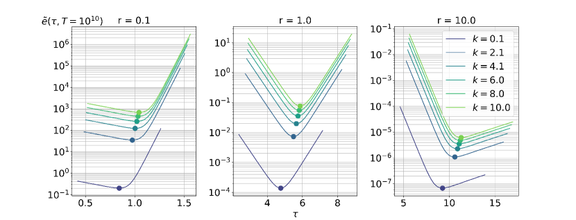
Figure 1: The mean squared error as a function of integration time $\tau$, for different values of the variables $k$ and $r$. The optimal value $\tau^{*}$ is marked on each of the plots.

From Eqs. 21 and 22, it can be seen that the least mean squared error, denoted by $\tilde{e}_{\rm min}(T):=\tilde{e}(\tau^{*}(T),T)$ can be reduced to a function of the variables, $k:=C_{\rm b}\gamma_{1}/C_{\rm var}$ and $r:=\gamma_{1}/\lambda_{1}$. Figure 1 shows the variation of $\tilde{e}(\tau,T)$ with $\tau$ at a fixed $T$, for different values of $k$ and $r$. It is clear that the mean squared error is high in magnitude when $r<1$ no matter the trajectory length, $\tau$. As expected for $r>1$, the optimal trajectory length increases with $r$ and leads to smaller mean squared errors. The mean squared error is large, as expected, both when a) $\tau$ is so short that variance is negligible, and the bias is significant and b) $\tau$ is large enough that the effect of exponential increase in the variance is clear. Thus we see a roughly parabolic shape centered at the optimal trajectory length for $r=1$, where the competing timescales are equal. The parabola is asymmetric $r<1$ because the time constant of the squared bias decay $(1/(2\gamma_{1}))$ is larger than that for the variance increase ($1/(2\lambda_{1})$). Thus, the bias drops more slowly when compared to $r\geq 1$, and upon increasing $\tau$, is overwhelmed very quickly by the dramatic increase in the variance, which is reflected in ${\tilde{e}(\tau,T)}$ for $\tau>\tau^{*}$. Analogously, the downward deflection of the right arm of the parabola for $r>1$, is explained by the fact that for values of $\tau>\tau^{*}$, we have a negligible bias and the exponential increase of the variance is slow, when compared to at $r=1$, while for $\tau<\tau^{*}$, increasing the trajectory length dramatically drops the bias but the variance remains small, and hence presents as a quick decline in the mean squared error. In 2Fig. 2a, $\tilde{e}_{\rm min}(T)/k$ is shown against the total computational cost $T$ at different values of $r$. The plots in 2Fig. 2a reveal that $\tilde{e}_{\rm min}$ is shifted upward on decreasing $k$ but the slope of $\tilde{e}_{\rm min}$ vs. T, is relatively unaffected by a change in $k$ when compared to a change in $r$. From 2Fig. 2a, we also observe that the least mean squared error $\tilde{e}_{\rm min}$ decays like an approximate power law of the total cost $T$. That is,

$$\tilde{e}_{\rm min}\sim{\cal O}(T^{-\beta})\;\;\text{ for some }\beta\equiv\beta(k,r)>0.$$ (23)

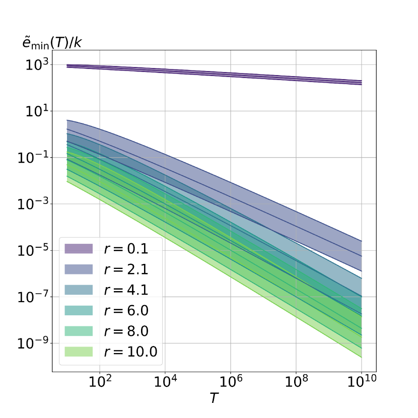
Fig. 2a $\tilde{e}_{\rm min}/k$ as a function of $T$, at different values of $r$.

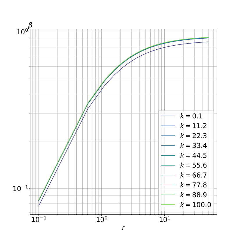
Fig. 2b Rate of convergence as a function of the ratio $r=\gamma_{1}/\lambda_{1}$.

In 2Fig. 2b, the rate of convergence $\beta$ is reported at different values of $r$ and $k$. From 2Fig. 2b, $\beta$ appears to be quite robust to varying the ratio of the bias to variance coefficients, $C_{\rm b}/C_{\rm var}$, when $\gamma_{1}$ is kept constant. On the other hand, it can be seen that the influence of the ratio of timescales $r$ is significant on the rate of convergence. For values of $r>1$, the least mean squared error falls faster than $1/\sqrt{T}$, for a range of values of $k$, indicating that convergence rates better than a typical Monte Carlo sampling can be achieved on choosing an optimal $\tau$ under the assumptions of section 3.2. This implies that, assuming a strongly chaotic system satisfying our optmistic estimates, when the timescale of the decay of bias is shorter than that of the growth of perturbations (1/$\lambda_{1}$), the ES method can be very efficient. On the contrary, 2Fig. 2b also indicates that the number of samples required to half $\tilde{e}_{\rm min}$ at $r=1$ must be increased four-fold while at $r=0.1$, a factor of $2^{10}$ increase in the number of samples is required to half the error. To summarize, even in the ideal case of exponential decay of the bias, a rate of decay smaller than the leading Lyapunov exponent, would lead to a significantly less efficient method than a typical Monte Carlo.

4 Numerical examples

The previous section was dedicated to a mathematical analysis of the convergence of the ES method. We were able to predict the best possible rates of convergence under suitable assumptions on the dynamics. In this section, we treat numerical examples of low-dimensional chaotic systems as well as simulations of turbulent flow. In each of the examples, our goal is to gauge, based on our numerical results, the applicability of the assumptions adopted in our analysis in section 3. When deemed applicable, we estimate the rate of convergence using our results from section 3 and discuss the computational tractability of the ES method given this rate. In other cases where either the analysis is inapplicable or the estimation of bias and variance is not practical, we use a physics-informed approach to predict the rate of convergence. The discussions following the numerical results delineate guidelines for determining the practicality of the ES method.

4.1 The Lorenz’63 attractor

As noted in the introduction, Eyink et al. [18] have performed a numerical analysis of the ensemble adjoint and related methods on the Lorenz’63 system and make several important observations regarding the convergence trends of $\theta_{\tau,N}$ in $\tau$ and in $N$. We choose the Lorenz’63 system as the first example in order to validate our present results against Eyink et al.’s. The Lorenz’63 system is a 3-variable model of fluid convection that is used as a classic example of chaos [31]. It consists of the following system of ODEs:

$$\frac{dx}{dt} =-\sigma x+\sigma y$$

$$\frac{dy}{dt} =-xz+sx-y$$

$$\frac{dz}{dt} =xy-bz,$$ (24)

with the standard values of $\sigma=10$, $b=8/3$ and $s=28$. These equations were derived by Lorenz and Saltzman [31] from the conservation equations for a fluid between horizontal plates maintained at a constant temperature difference. The phase vector $u:=[x,y,z]^{T}$, whose evolution these equations describe, corresponds to coefficients in the Fourier series expansion of the stream function and the temperature profile. The parameter $s$ is the Rayleigh coefficient normalized by the critical value above which flow instabilities develop. The objective function of our interest is $J(u(t)):=z(t)$ which is proportional to the deviation of the temperature from the linear profile that would be achieved if the fluid were static. It is well-known that a compact attractor exists in phase space.

We use the algorithms described in section 2.2 to compute all three types of ES estimators $\theta_{\tau,N}^{\rm FD}$, $\theta_{\tau,N}^{\rm A}$ and $\theta_{\tau,N}^{\rm T}$. To ensure that the initial condition is sampled from the steady-state distribution on the Lorenz attractor, the system is evolved for a spin-up time of about $1.1$ time units, before we start computing the sensitivities. This spin-up time is estimated as $1/\lambda_{1}$, with $\lambda_{1}\approx 0.9$ known from the literature to be the largest Lyapunov exponent. The true value of the sensitivity $(d\mu_{s}(J)/ds)$ was computed by Eyink et al. [18] to be $\approx 0.96$. This value is obtained by numerically computing $\mu_{s}(J)$ as an ergodic average at a range of values of $s$. It can be seen that $\mu_{s}(J)$ turns out approximately to be a straight line with a slope of 0.96 around $s=28$. The primal, the tangent and adjoint dynamics in equations 24, 3 and 5 respectively are computed using forward Euler time integration with a timestep of $0.005$ time units. The computational cost $T=N\tau$ was chosen to be 5000 time units. The estimators were computed for a range of values of $\tau$ up to 3 time units. In order to apply our analysis in section 3, we wish to numerically estimate the bias and variance of $\theta_{\tau,N}$. We estimate $\mu_{s}(\theta_{\tau,N})$ as a sample average of $\theta_{\tau,N}$ using 5 million independent samples. That is, we approximate $\mu_{s}(\theta_{\tau,N})$ as $\theta_{\tau,5\times 10^{6}}$ while the true value is not a function of the number of samples but only of $\tau$. The variance of $\theta_{\tau,N}$ is again approximated as a sample average wherein $\mu_{s}(\theta_{\tau,N})$ is replaced with its estimate $\theta_{\tau,5\times 10^{6}}$.

4.1.1 Empirically determined upper bound for rate of convergence

Our overarching goal is to predict the rate of convergence of the ES method. We now discuss that it is possible to roughly estimate the rate based on numerical results at a fixed computational cost $T$. In Lea-Allen-Haine’s application of the ES method on the Lorenz’63 system [14], $\tau=1$ is used to obtain an accurate estimate of $d\mu_{s}(J)/ds$; for the sake of comparison with their results, we estimate the rate of convergence locally around $\tau=1$. To obtain the rate of convergence, we obtain estimates, for the exponential rates of increase and decrease of the variance and the bias respectively, from our numerical results. Then, we use 2Fig. 2b to obtain the rate of convergence from the ratio of these obtained rates.

First we establish an empirical estimate for the variance rate. Our numerical estimates for the bias and variance of the estimators $\theta_{\tau,N}^{\rm A},\theta_{\tau,N}^{\rm T}$ and $\theta_{\tau,N}^{\rm FD}$ computed as described above, are shown in 3Fig. 3a. In 3Fig. 3b, the numerical estimates of $\mu_{s}(\theta_{\tau,N}^{2})$ are shown for all three estimators. Ignoring transient behavior for $\tau$ up to $\sim 0.5$, the asymptotic exponential rate of the variance estimate, obtained by determining the slope from 3Fig. 3a, is larger than the $2\lambda_{1}$ rate that we predicted in 3.3. To understand this result, let us assert that our numerical estimate of the variance reflects the trend of the true variance and the CLT holds for the given range of values of $\tau$. If the first assertion holds, the true variance is increasing exponentially at a faster rate than $2\lambda_{1}$. Now, owing to the convergence of Ruelle’s formula, we know that $\mu_{s}(\theta_{\tau,N})$ cannot have an unbounded growth as a function of $\tau$ and therefore, the rate of increase of ${\rm var}(\theta_{\tau,N})$ must be captured by that of $\mu_{s}(\theta_{\tau,N}^{2})$. Computing the slope from 3Fig. 3b, we see that the numerical estimate of $\mu_{s}(\theta_{\tau,N}^{2})$ is indeed exponential in $\tau$ at the rate $\sim 2\times 0.85$ for both the tangent and adjoint estimators, from a least-squares fit. This value of the rate is closer to our theoretical prediction of $2\lambda_{1}$. Therefore, it is reasonable to conclude that neither of our previously stated assertions holds true. As a result, we have considerable error in our estimates of $\mu_{s}(\theta_{\tau,N})$ and $\mu_{s}(\theta_{\tau,N}^{2})$ since the error is decaying slower than expected from CLT. Since both these errors play a role in the variance estimation, obtaining the rate of increase from the estimate of $\mu_{s}(\theta_{\tau,N}^{2})$ is more accurate. It is thus reasonable to take the better numerical estimate, $2\times 0.85$, as the rate of exponential increase of the variance for $\tau$ up to 1.5.

In 3Fig. 3a, we obtain from the slope of the bias term (again using a least-squares fit) for $\tau\leq 1.5$, the rate $\gamma_{1}\sim 1.3$. Therefore, we obtain $r=1.3/0.85=1.5$ as the rough estimate needed to determine the rate of convergence under our model assumptions in sec 3.3. Thus, we note from 2Fig. 2b that $\beta\sim 0.5$. It would not be gainful to also estimate $k$ since we only seek an upper bound for $\beta$ which is quite insensitive to $k$, in the first place. We can interpret this rate as the best possible rate of convergence for the Lorenz’63 system.

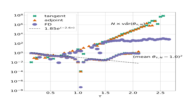
Fig. 3a Estimates of the variance and the bias of $\theta_{\tau,N}$ as a function of $\tau$, for the Lorenz’63 system outlined in section 4.1. The dashed line indicates the least-squares fit over $\tau\leq 1.5$.

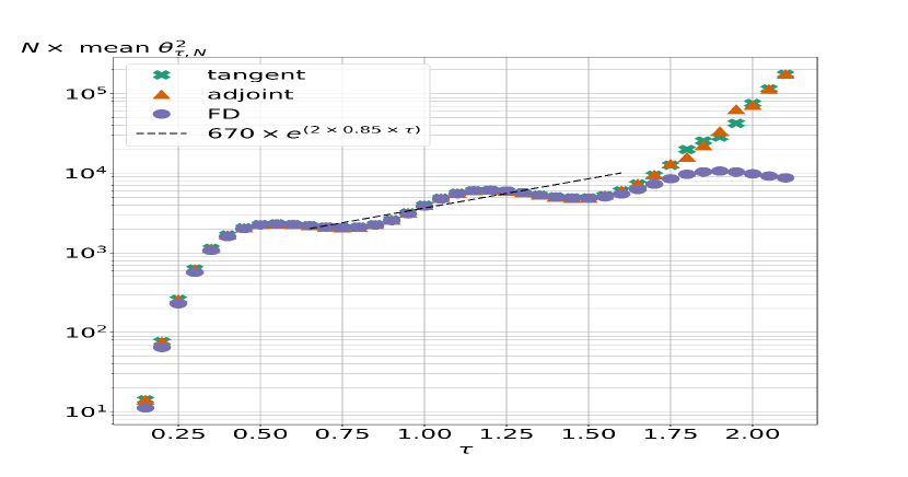
Fig. 3b Sample mean estimates of $\mu_{s}(\theta_{\tau,N}^{2})$ as a function of $\tau$ for the Lorenz’63 system outlined in section 4.1. The dashed line indicates the least-squares fit over $\tau\leq 1.5$.

4.1.2 Agreement with Eyink et al.’s results

Eyink et al. [18] propose that the probability distribution of $\theta_{\tau,N}$ for the Lorenz’63 system is a fat-tailed distribution and does not obey the classical CLT. Consequently, our assumption of bounded variance of $\theta_{\tau,N}$ for finite values of $\tau$ should fail for this system. Our numerical results indicate that both the variance and bias trends are worse than our optimistic model, thus confirming their predictions. However, locally around $\tau\sim 1$, operating under the assumption that the bias and the variance trends can be empirically modelled using our optimistic estimates, we were able to provide an upper bound on the actual convergence rate. Owing to the fact that $\tau\sim 1$ is not large enough for the failure of the CLT assumption to be manifest, our empirically determined rate of 0.5 provides an upper bound on that estimated using Eyink et al.’s tail estimates. Thus we conclude firstly that our numerical results provide further evidence in support of the failure of the CLT for $\theta_{\tau,N}$. Secondly, empirical determination of the optimistic rate of convergence under the CLT assumption locally around $\tau\sim 1$, predicts an upper bound at the rate of a Monte Carlo simulation, confirming Eyink et al.’s observations.

It is worth commenting on the fundamental difference between the distribution of sample averages of state functions and that of $\theta_{\tau,N}$, which is a sample average of the derivative of a state function (averaged over a short time). The former distribution has bounded variance but the latter is not guaranteed to, as this example demonstrates. In fact, it has been shown [32] that $N$-sample averages (computed numerically as ergodic averages) of state functions converge at the rate of $1/\sqrt{N}$. However, the behavior of the $N$-sample average that is $\theta_{\tau,N}$, is unlike that of state functions. $\theta_{\tau,N}$ converges to $\mu_{s}(\theta_{\tau,N})$ (due to the law of large numbers) at a rate slower than $1/\sqrt{N}$. This rate decreases as $\tau$ increases, bearing on the poor accuracy of the estimate $\theta_{\tau,5\times 10^{6}}$ for values of $\tau\gtrsim 1.5$ seen in 3Fig. 3a, despite using a seemingly large number of samples.

Another observation that can be made from 3Fig. 3a is that unlike the variances of $\theta_{\tau,N}^{\rm A}$ and $\theta_{\tau,N}^{\rm T}$, ${\rm var}(\theta_{\tau,N}^{\rm FD})$ appears to saturate for $\tau\gtrsim 1.5$. This is explained by the fact that $\left|\theta_{\tau,N}^{\rm FD}\right|$ is bounded above by $\left\lVert J\right\rVert_{\infty}/\epsilon=c/\epsilon$, where $\epsilon$ is the value of the parameter perturbation in the finite difference approximation. The value $c$ is the supremum of the $z$ coordinate of the Lorenz attractor, which is a finite value since the attractor is a bounded set. The fact that $\theta_{\tau,N}^{\rm FD}$ is bounded for all $\tau$ can also be observed in the saturation of the estimate of $\mu_{s}(\theta_{\tau,N}^{\rm FD^{2}})$ shown in 3Fig. 3b.

4.2 The Lorenz’96 model

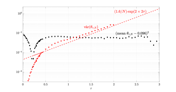
Figure 4: The variance and the square of the bias in the ensemble tangent sensitivity estimator for the Lorenz’96 system. The dashed line indicates the least-squares fit of the variance data.

Our results for the Lorenz’63 system in section 4.1 show that an upper bound on the rate of convergence for an optimal choice of $\tau$ ($\sim 1$) is $0.5$. Although the actual rate is slower than a typical Monte Carlo simulation, one can immediately see that since the system is low-dimensional, ES is still practical in the Lorenz’63 system. In this section, we aim to assess the computational practicality of the ES method in a higher-dimensional system. We consider the atomspheric convection model, called the Lorenz’96 [33] model, that is known to have a strange attractor [34]. The 40-dimensional state vector $u:=[x_{1},\cdots,x_{40}]^{T}$ evolves according to the following set of odes [33, 34]

$$\frac{dx_{k}}{dt}=(x_{k+1}-x_{k-2})x_{k-1}-x_{k}+s,\;\;k=1,\cdots,40,$$ (25)

where, $s$, the parameter of interest, denotes an external driving force. The first term on the right hand side of equation 25 represents nonlinear advection and the second term represents a viscous damping force. The components of the state vector are periodic in the sense that $x_{k}=x_{40+k},\;\;k\in\mathbb{N}$. We define our objective function $J(u(t))$ to be the mean of the components of $u$, i.e.,

$$J(u(t))=(1/40)\sum_{k=1}^{40}x_{k}(t).$$

We use the value $s=8.0$ for the forcing term, at which the system has been shown to exhibit chaotic behavior [34]. Time integration of the primal system of equations 25 is performed using a fourth order Runge-Kutta scheme with a timestep of 0.01 time units. The distribution of each component of the state vector for this system is known from the literature [35] to converge to a Gaussian and the time average of $J$ approximately becomes a linearly varying function with $s$, on long-time evolution. The slope of $\mu_{s}(J)$ vs. $s$ estimated from our computations and previous work [34] is $0.096$.

In Fig. 4, we report the squared bias and the variance of the estimator $\theta_{\tau,N}^{\rm T}$ as a function of $\tau$. The total cost, $T$, is set at $10^{4}$ time units across different values of $\tau$. The values of $\mu_{s}(\theta_{\tau,N})$ and $\mu_{s}(\theta_{\tau,N}^{2})$ are computed as sample means and used in the approximation of the bias and variance (denoted by $\hat{\rm var}(\theta_{\tau,N})$ in Fig. 4 to indicate the approximation as a sample mean) terms, identical to our description in section 4.1 for the Lorenz’63 system. From Fig. 4, we can see that the variance follows our model assumptions in section 3.2; we find that the variance is exponential in $\tau$ at the rate $\approx 4$, which is close to twice the leading Lyapunov exponent reported in the literature [34, 35]. From Fig. 4, ignoring initial transients, it can be seen that the bias term does not show an exponential convergence, not even locally in the vicinity of $1/\lambda_{1}\approx 0.5$. As a result, our local analysis to produce a rough estimate under our model assumptions, as we did in section 4.1, is not applicable in this case. This implies that the rate of convergence is worse than our model in 3.2 (for any $r$) since the bias falls slower than the assumed exponential. One can argue that the mean squared error (sum of the squared bias and the variance) is low in absolute value for $\tau$ near 0.5 deeming the ES estimator to be reasonably accurate and therefore practically applicable, although the asymptotic rate of convergence in $\tau$ may be low. However, note that the rate of convergence is an objective function-independent measure of the ES estimator – the mean squared error may be coincidentally within required accuracy for a choice of $\tau$, for this particular objective function. Thus, it is reasonable to conclude that the ES method is infeasible for the Lorenz’96 model.

4.3 Chaotic flow over an airfoil

In this example, we discuss the numerical simulation of an unsteady, chaotic flow around a two-dimensional airfoil. So far, we have assessed the convergence of the ES method by observing the trends in the bias and variance of $\theta_{\tau,N}$ in low-dimensional systems. Our numerical results were informative enough to predict the rate of convergence while simultaneously being within the limits of practical computation, owing to the low dimensionality of the systems considered in sections 4.1 and 4.2. In contrast, in a typical chaotic CFD simulation, it would not be practical to numerically estimate the bias and variance trends of $\theta_{\tau,N}$. We will thus attempt to predict the convergence trend using a single finite-difference solution (that can be used to compute one sample of $\theta_{\tau,N}$ ). Our goal is to use a physics-based approach that eliminates the need for a rich $\theta_{\tau,N}$ dataset. We consider the NACA 0012 airfoil at the Reynolds number $Re_{\infty}=2400$ and Mach number $M_{\infty}=0.2$ at an angle of attack $\alpha=20^{\circ}$. Although the flow physics in three-dimensional turbulent flows is more complex, the two-dimensional airfoil case we consider exhibits the phenomena of stall and flow separation that are responsible for the chaotic behavior. For an extensive analysis of the Lyapunov spectrum and its dependence on the numerical discretization for this problem, see [36, 37].

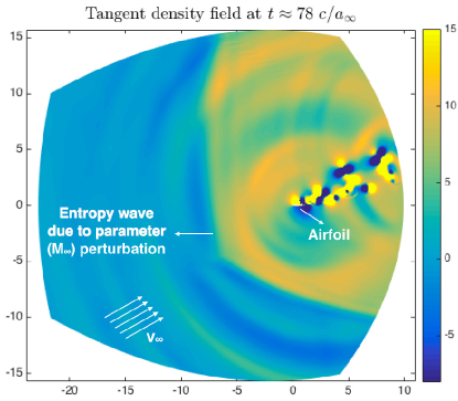
Figure 5: Tangent density field $v_{\rho}$ at time $t=78\,c/a_{\infty}$.

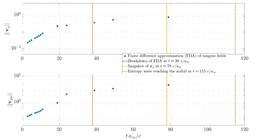
Figure 6: Time evolution of $L^{2}$ norm of the tangent fields corresponding to the density ${\rho}$ (top) and $x$-momentum ${\rho u}$ (bottom).

The primal system is the set of compressible Navier-Stokes equations, which is discretized in space using a third-order Hybridizable Discontinuous Galerkin (HDG) method [38, 39] with the Lax-Friedrichs-type stablization matrix in [40]. The computational domain spans $\sim 10-20$ chord lengths away from the airfoil and is partitioned using an O-grid with 35280 isoparametric triangular elements. The use of a large computational domain is customary in external aerodynamics to reduce the change in the effective angle of attack induced by the missing vortex upwash. The state vector $u$ is defined to be the set of coefficients in the basis function representation of the density, the components of the momenta and the energy, at all elements in the computational domain. Our objective function $J$ is the lift coefficient and the parameter of interest $s$ is the freestream Mach number, $M_{\infty}$. A three-stage, third-order diagonally-implicit Runge-Kutta (DIRK) method [41] is used for the temporal discretization. A no-slip, adiabatic wall boundary condition is imposed on the airfoil surface, and the characteristics-based, non-reflecting boundary condition in [38, 39] is used on the outer boundary. The spin-up time before the sensitivity computation is performed is $t=10,000\,c/a_{\infty}$, where $a_{\infty}$ denotes the far-field speed of sound and $c$ is the chord length. We note that the chosen spin-up time is one order of magnitude larger than the time required for the convergence of time-averaged flow quantities [36]. At the spin-up time, we reset $t=0$ and all the results below are indicated with respect to this new initial time.

Since a tangent solver is not available typically in CFD codes, the tangent perturbation fields denoted by $v(t)$ are computed non-intrusively with regard to the primal solver using a finite difference approximation (FDA). The parameter perturbation has a magnitude of $\epsilon=10^{-6}$. Fig. 5 shows the sensitivity field of the fluid density with respect to the perturbation in the freestream Mach number at time $t=78\,c/a_{\infty}$. This quantity, denoted in Fig. 6 as $v_{\rho}$, can be used to compute a single sample of $\theta_{\tau,N}^{\rm FD}$. The airfoil, much smaller in size than the computational domain, is annotated in Fig. 5. Entropy and acoustic waves are generated on the outer boundary at $t=0$ due to the $M_{\infty}$ perturbation. From the entropy wavefront shown in Fig. 5, one observes that the entropy wave does not reach the airfoil yet at $t=78c/a_{\infty}$. The time evolution of the $L^{2}$ norm of the tangent fields corresponding to the density, $v_{\rho}$, and the $x$-momentum, $v_{\rho u}$, are shown in 6. As we discussed in section 4.1, finite difference sensitivities tend to saturate with time as opposed to tangent and adjoint sensitivities which keep increasing exponentially. This is due to the finite difference sensitivities having an upper bound proportional to $1/\epsilon$, since the supremum of the objective function over phase space is a finite value independent of time. As indicated in Fig. 6, the entropy wave reaches the airfoil at $t\sim 115\,c/a_{\infty}$. By this time, the sensitivity fields already saturate. We can estimate by extrapolation that $\left\lVert v_{\rho}\right\rVert,\left\lVert v_{\rho u}\right\rVert>10^{5}$ if computed using the tangent equation, at $t=115\,c/a_{\infty}$.

One expects the bias in the ES estimator to be non-negligible for trajectory lengths shorter than $t=115\,c/a_{\infty}$. That is, the sensitivities must be computed at least until the time the information about the perturbation propagates to the airfoil, in order for the average sensitivity of the lift to converge to its true value. In other words, convergence of the bias requires the entropy wave to reach the airfoil and thus $\tau$ must be larger than $\tau^{*}:=115\,c/a_{\infty}$. In order to predict the cost of the ES method, let us make the optimistic assumptions that at $\tau^{*}$, the bias term is close to zero and that the CLT holds for the variance. A random tangent field is at least $\sim 10^{5}$ in magnitude at $\tau^{*}$ implying that the variance at $\tau^{*}$ would be ${\cal O}(10^{10})$. Therefore, under the CLT assumption, which we have shown to be too optimistic in our previous examples in sections 4.1 and 4.2, one would require on the order of $10^{10}$ samples for an ${\cal O}(1)$ mean squared error. Solving the primal and the perturbation equations on the order of 10 billion times for trajectories of lengths $\tau^{*}$ would be computationally infeasible. This example illustrates that the much shorter timescale of divergence of the adjoint/tangent fields, compared to that of the convergence of the bias, leads to computational intractability of the ES method.

4.4 Turbulent flow over a turbine vane

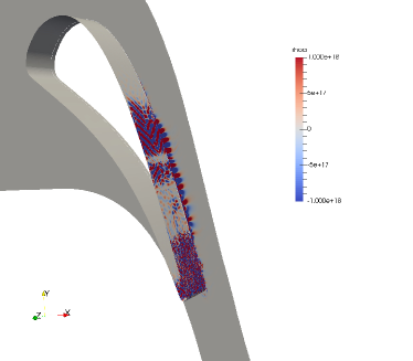
Fig. 7a Adjoint field corresponding to the density, labelled rhoa in the colormap, at $t^{*}=0.35$.

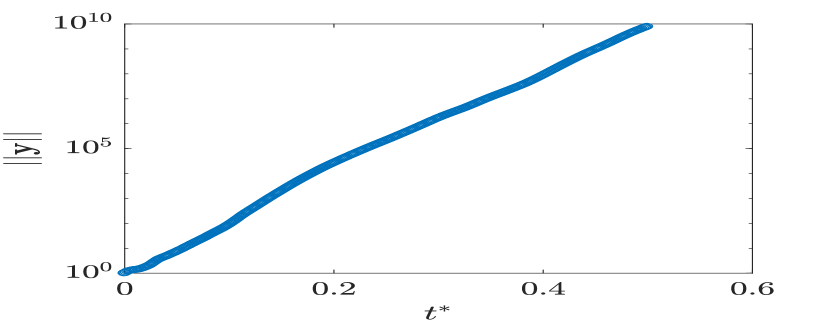
Fig. 7b The $L^{2}$ norm of the adjoint vector field, $y$, for the Navier-Stokes system in section 4.4 as a function of time.

As a final example, we consider an implicit LES of turbulent flow around a highly loaded turbine nozzle guide vane performed by Talnikar et al. [42]. Our simulations approximate the aero-thermal experimental investigations of turbine guide vanes in a linear cascade arrangement at the von Karman Institute for Fluid Dynamics [43]. The linear cascade is approximated in the simulation domain using periodic boundary conditions in the transverse and spanwise directions. The spanwise extent, is restricted to $0.15$ times the chord length, which has been numerically verified to be sufficient to capture the turbulent flow physics. The Reynolds number of the flow is $10^{6}$. The isentropic Mach number computed with respect to the static pressure at the outlet is 0.9. Isothermal boundary condition is used on the surface of the vane. The fluid achieves transonic speeds as it flows over the surface of the vane, transitioning to turbulence on the suction side.

The primal problem is a compressible Navier-Stokes system as in 4.3, solved here using a second order finite volume scheme [42]. A strong stability-preserving third order Runge-Kutta scheme is used for time integration and a weighted essentially non-oscillatory scheme [44] is used for shock capturing. The mesh is generated by uniformly extruding a two-dimensional hybrid structured/unstructured mesh in the spanwise direction.

The long-time averaged objective of interest is the mass-flow averaged pressure loss coefficient on a plane 0.25 chord lengths downstream of the trailing edge of the vane. The reduction in stagnation pressure loss is due to mixing in the turbulent wake and the formation of a boundary layer on the surface of the vane. Sensitivities (computed using the adjoint method) are calculated with respect to Gaussian-shaped source term perturbations to the system dynamics centered $0.3$ chord lengths upstream from the leading edge of the vane in the axial direction. The time variable, $t^{*}$, is nondimensionalized with respect to the flow-through time, which is the duration of the time taken for fluid flow from the inlet to outlet. In 7Fig. 7a, we show the adjoint field corresponding to the density, denoted by rhoa, at $t^{*}=0.35$. 7Fig. 7b shows the $L^{2}$ norm of the adjoint field, denoted by $y$, as a function of $t^{*}$. From the growth of the adjoint vectors in 7Fig. 7b, we can estimate the leading Lyapunov exponent for the flow to be $\sim 46$ in nondimensional units. The time taken for the entropy wave of the adjoint solution to reach the source of the perturbation (the propagation direction of the adjoint solution is reversed with respect to the primal flow) is $\gtrsim 0.5$ time units. From 7Fig. 7b, we can see that the adjoint solution has diverged by $10$ orders of magnitude by this time.

The reason for the rapid divergence is the high angle of attack of the flow onto the vane surface which causes the Mach wave of the adjoint solution to propagate with a maximum speed of Mach 1.9 upstream in the axial direction. The entropy wave, in comparison, has a lower maximum speed of Mach 0.9, which is equal to the flow speed. The adjoint diverges quickly once the Mach wave reaches the turbulent boundary layer region close to the trailing edge of the vane on the suction side, as shown in 7Fig. 7a. But the bias in the adjoint computed over an ensemble of trajectories can be expected to decline only for trajectory lengths $\gtrsim 0.5$ time units, which is approximately the time required for the entropy wave to reach the vane leading edge. Similar to the flow over the airfoil presented in section 4.3, the lower speed of propagation of the entropy wave from the inlet makes the ES method infeasible in this problem.

Equipped with the estimate of the Lyapunov exponent and the timescale of convergence of the bias, we predict the cost of the ES method in this case. As in section 4.3, let us assume the best case scenario for both the bias and the variance terms. Suppose the bias has negligible magnitude at $0.5$ time units and that the CLT assumption is valid. Since the true variance would be on the order of $10^{20}$ at $t^{*}=0.5$, we would require ${\cal O}(10^{20})$ samples in order to reduce the variance of $\theta_{0.5,N}^{\rm A}$ and consequently, the mean squared error to ${\cal O}(1)$. To roughly estimate the computational power required, we need about $10$ teraFLOPS for $12$ hours for a single adjoint simulation up to $t^{*}=0.5$; this means approximately $10^{15}$ exaFLOPS for $12$ hours would be needed for convergence. This is beyond the computational capabilities achievable in the near future. To conclude our discussion, even though the source of perturbations is close to the leading edge of the vane, turbulence at a high Reynolds number makes the timescale of the growth of perturbations much shorter than the time required for the propagation of the information about the perturbation through entropy waves. As a result, since the number of samples required for convergence increases exponentially at best with time, the ES method becomes computationally intractable.

Before closing, we remark on the differences between this example and the previous one in section 4.3. Although the timescale discrepancy argument supplied to rule out the applicability is the same in the two examples, the appearance of such a discrepancy is attributed to rather different reasons. In the airfoil flow, one could have argued that the particular choice of the parameter perturbation prolonged the timescale for the decay of the bias, leading to the divergence of the tangent/adjoint within that timescale. That situation is typical in an external flow, where parameters we can influence are at the farfield, spatially separated from quantities of interest. The flow over the turbine vane in this section, on the other hand, is an internal flow where the flow physics (the slowness of the mean flow compared to the Mach wave) was responsible for the inapplicability of the ES method, rather than the limited choice of controllable parameters.

5 Discussion and comments

From the optimistic analysis presented in section 3 and the numerical examples considered in the previous section, one can conclude that the ES method cannot be a universal chaotic sensitivity analysis method, owing to its computational cost. The main basis for this conclusion is that the ES estimator’s bias often decays at a longer timescale than the inverse of the largest Lyapunov exponent, which dictates its variance. The analyses and the examples do not preclude however, cases where this timescale discrepancy is not large enough to make the ES method computationally impractical. This leads to the question of whether one can choose specific objective functions and parameters, that are dissimilar to the examples in section 4, so as to yield better scenarios for the application of the ES method. Here we provide a closer examination of this difficult and problem-specific question; we draw upon connections between signature timescales, that could guide us in the determination of the edge cases for the method’s applicability.

As noted in section 3, in uniformly hyperbolic systems that we consider here, the decay of correlations is exponential. Using the Collet-Eckmann conjecture, we argued that the rate of the bias decay ($=\gamma_{1}$) is similar to the rate of correlation decay. This argument is also exemplified, in addition to our heuristic explanation considering only stable perturbations in section 3.2, through alternative derivations of Ruelle’s response formula that have appeared in a few works in the dynamical systems literature ([45, 46]; see also [47] or proposition 8.1 of [48] for a computable modification of Ruelle’s formula in discrete-time systems). The thrust of these alternative formulations is that one can replace the computation of Ruelle’s formula which, in its original form (Eq. 8) is a time integral with an exponentially increasing variance, with a computation that has bounded variance at all times. These formulae have the convergence of a typical Monte Carlo estimator (at the rate of $1/\sqrt{N}$), independent of the objective function, and the bias in these formulae decay as the time correlations in the system. This implies that, supposing $\theta_{\tau,N}$ behaved like a Monte Carlo estimator for a specific objective function (or only slightly worse, as in the Lorenz’63 case), the bias decay rate is still bounded above by the correlation decay rate.

It seems unintuitive that there exists a connection between the two timescales. After all, the two exponential rates, of the decay of correlations and that of the Lyapunov exponents, represent disconnected chaotic phenomena, namely, the rate of loss of information carried by state functions, and local expansion of infinitesimal perturbations, respectively. Nevertheless, several works have verified this connection in low-dimensional uniformly hyperbolic dynamics (see [49, 50] for recent work). In fact, numerical studies in disparate turbulent flows such as drift wave turbulence in plasma [51] and in fluid convection [52], also confirm that the correlations decay slower than $(1/\lambda_{1})$. Given the validity of the chaotic hypothesis in many turbulent flows, there is reason to expect this connection between the two timescales, that can be rigorously shown to hold only in mathematical toy models, to also manifest itself in general turbulent flows.

At the same time, the rate of correlation decay depends on the observables considered; this is why one cannot exclude the existence of objective function-parameter pairs that lead to fast convergence of $\theta_{\tau,N}$, even though the decay of correlations for the system as a whole is at a slower rate than $\lambda_{1}$ (i.e., even if the above conjecture holds). The decay rate of correlations for a chaotic system is generally determined as the average decay between two functions belonging to a broad function class (such as the set of continuously differentiable functions of the state). There exist observables correlations between which decay at a faster rate than that given by this signature rate of the system. The correlation time at which the bias converges is rather difficult to predict a priori. In accordance with the approach of this work which isolates extreme scenarios, we can take the autocorrelation times of the worst-case observables (or the ones with notably slow decay rates) as a crude approximation of the upper bound on the bias decay time. In the event that this upper bound is smaller than the inverse of the largest Lyapunov exponent, we can expect the ES method to behave at least as well as a Monte Carlo estimator.

In aeroacoustics, an important application area where RANS modeling is inadequate and turbulence-resolving LES/DNS is resorted to, farfield noise (away from a nozzle) caused by a turbulent jet is often used as an objective function. In such a scenario, a wealth of spectral studies (for brevity, we refer only to a few recent works on modelling turbulent jets [53, 5, 54]) have found that the energy-carrying spatial Fourier modes (of lower wave number) appear as large-scale structures with high spatial coherence. This also translates into high coherence in time or equivalently, a slow decay of time correlations of streamwise observables – this being corroborated by more sophisticated mechanisms of turbulent structure transit than the oft-used Taylor’s hypothesis of frozen turbulence (among the vast body of work on space-time correlations in turbulent flow, we point the reader to some comprehensive reviews in [55, 56, 57] that detail this point). So, in this case, we can take the integral timescales reported for farfield streamwise measurements as the worst-case estimate for the bias decay time. Similarly, in turbulent boundary layers, integral timescales associated with the intermittent or outer regions of the flow can be taken as an upper bound since very near-wall regions exhibit faster decay of correlations. In the case that the slowest rate of correlation decay estimated as the inverse of this upper bound, is still larger than the largest Lyapunov exponent, the ES method could be practical.

Given an objective function of interest and a fixed set of parameters, one might in practice, benefit from knowing the decay of correlations from thorougly documented computational DNS/LES datasets or experimental observations for the appropriate type of flow (for example, see [54, 53, 5] for the case of jets and [58, 59, 60] for the case of turbulent boundary layers). In this regard, the availability of space correlation data, which are more naturally obtained and commonly reported in computational studies, should also prove to be sufficient for estimation purposes since they can be transformed approximately to time-correlation data. If an estimate of the largest Lyapunov exponent is also available, one needs to simply compare the timescales and use the results of section 3 to predetermine if the ES method would be applicable.

Ultimately, these heuristic predictions based on prior knowledge of timescales can only help us identify the corner cases of applicability (or the lack thereof) of the ES method. We contend that it is more likely to encounter undecidable cases and close this discussion with such an example that appears in Rayleigh-Bénard convection. Sirovich et al. [52] have shown that the correlation time defined as the time it takes for the streamwise velocity autocorrelations to drop to its first minimum, is on the same order of magnitude as the largest Lyapnov exponent. Interestingly, our numerical results for the Lorenz’63 system (section 4.1), which is a mathematical model for Rayleigh-Bénard convection, is also in line with this finding – the rate of decay of the bias and the largest (and only) positive Lyapunov exponent are both ${\cal O}(1)$. In such a scenario, the practitioner may choose to rely on alternative methods [13, 47, 21, 22] in order to avoid incurring the cost of solving an enormous number of tangent or adjoint equations without being to establish convergence.

6 Conclusion

To compute sensitivities with respect to design parameters, of statistically stationary quantities in chaotic systems, ensemble methods appear to be an appealing solution; they are both conceptually simpler and easier to implement than fluctuation-dissipation-based [21] and shadowing-based [20] methods, all of which are, moreover, still under active development. However, the present work has shown that Eyink et al.’s [18] results revealing poor convergence of ensemble computations in the Lorenz’63 system, is more widely representative of convergence trends in general chaotic systems. The present work deals with estimating a theoretical upper bound on the rate of convergence of an ensemble sensitivity, agnostic to the objective function-parameter pair.

For this, the most optimistic assumptions are made on the bias and variance associated with the ensemble sensitivity (ES) estimator, under the mathematical simplification of uniform hyperbolicity. We show that, with the integration time, in the best case, the bias decays exponentially at a problem-dependent rate and the variance increases exponentially at the rate of twice the largest Lyapunov exponent. Assuming these optimistic bounds, the computational cost of the ES method, in theory, still scales exponentially with the mean squared error. The ratio of the bias decay rate to the leading Lyapunov exponent of the system, is the single most influential parameter that determines the feasibility of the method.

Our numerical results for the Lorenz’63 system show that the optimistic model proposed for the least mean squared error is only locally applicable. The upper bound on the rate of convergence is 0.5, concurring with Eyink et al.’s [18] results. The 40-variable Lorenz’96 system serves as an example of a low-dimensional attractor for which the asymptotic convergence is remarkably slow. Although the rate of convergence is poor for this system, the mean squared error magnitudes were low at a reasonable computational cost, for the chosen objective function. This suggests that one may encounter, in practice, objective functions for which the ensemble sensitivities are within a specified accuracy, at an affordable computational cost. In the numerical simulations of chaotic fluid flow we consider, we obtain optimistic estimates on the rate of convergence which hold true for a general objective function. Our results indicate that the flow physics imposes an upper bound on the rate of convergence. Altogether, the present numerical evidence suggests the following: even under the optimistic assumption of exponential decay of the bias, the cost of exponential sampling of an expensive primal problem can make the ES method infeasible in practical applications, for a general objective function-parameter pair. However, there may exist objective function and parameter choices that lead to a smaller timescale discrepancy between the bias decay and the variance increase – this could lead to a faster convergence than the estimate of the upper bound.

Funding Sources

This work was supported by AFOSR Award FA9550-15-1-0072 under Dr. Fariba Fahroo and Dr. Jean-luc Cambier.

References

- Palacios et al. [2012] Palacios, F., Duraisamy, K., Alonso, J. J., and Zuazua, E., “Robust grid adaptation for efficient uncertainty quantification,” AIAA journal, Vol. 50, No. 7, 2012, pp. 1538–1546. 10.2514/1.J051379.
- Wang et al. [2012] Wang, Q., Duraisamy, K., Alonso, J. J., and Iaccarino, G., “Risk assessment of scramjet unstart using adjoint-based sampling methods,” AIAA journal, Vol. 50, No. 3, 2012, pp. 581–592. 10.2514/1.J051264.
- Fidkowski and Darmofal [2011] Fidkowski, K. J., and Darmofal, D. L., “Review of output-based error estimation and mesh adaptation in computational fluid dynamics,” AIAA journal, Vol. 49, No. 4, 2011, pp. 673–694. 10.2514/1.J050073.
- Rizzetta and Visbal [2003] Rizzetta, D. P., and Visbal, M. R., “Large-eddy simulation of supersonic cavity flowfields including flow control,” AIAA journal, Vol. 41, No. 8, 2003, pp. 1452–1462. 10.2514/2.2128.
- Bodony and Lele [2008] Bodony, D. J., and Lele, S. K., “Current status of jet noise predictions using large-eddy simulation,” AIAA journal, Vol. 46, No. 2, 2008, pp. 364–380. 10.2514/1.24475.
- Engblom et al. [2004] Engblom, W., Khavaran, A., and Bridges, J., “Numerical prediction of chevron nozzle noise reduction using WIND-MGBK methodology,” 10th AIAA/CEAS Aeroacoustics Conference, 2004, p. 2979. 10.2514/6.2004-2979.
- Tucker [2004] Tucker, P. G., “Novel MILES computations for jet flows and noise,” International Journal of Heat and Fluid Flow, Vol. 25, No. 4, 2004, pp. 625–635. 10.1016/j.ijheatfluidflow.2003.11.021.
- Peter and Dwight [2010] Peter, J. E., and Dwight, R. P., “Numerical sensitivity analysis for aerodynamic optimization: A survey of approaches,” Computers & Fluids, Vol. 39, 2010, pp. 373–391. 10.1016/j.compfluid.2009.09.013.
- Giles and Pierce [2000] Giles, M. B., and Pierce, N. A., “An introduction to the adjoint approach to design,” Flow, turbulence and combustion, Vol. 65, 2000, pp. 393–415. 10.1023/A:1011430410075.
- Giles et al. [2003] Giles, M. B., Duta, M. C., M-uacute, J.-D., ller, and Pierce, N. A., “Algorithm developments for discrete adjoint methods,” AIAA journal, Vol. 41, No. 2, 2003, pp. 198–205. 10.2514/2.1961.
- RA Martins et al. [2004] RA Martins, J. R., Alonso, J. J., and Reuther, J. J., “High-fidelity aerostructural design optimization of a supersonic business jet,” Journal of Aircraft, Vol. 41, No. 3, 2004, pp. 523–530. 10.2514/1.11478.
- Nielsen and Anderson [1999] Nielsen, E. J., and Anderson, W. K., “Aerodynamic design optimization on unstructured meshes using the Navier-Stokes equations,” AIAA journal, Vol. 37, No. 11, 1999, pp. 1411–1419. 10.2514/2.640.
- Ni and Wang [2017] Ni, A., and Wang, Q., “Sensitivity analysis on chaotic dynamical systems by Non-Intrusive Least Squares Shadowing (NILSS),” Journal of Computational Physics, Vol. 347, 2017, pp. 56–77. 10.1016/j.jcp.2017.06.033.
- Lea et al. [2000] Lea, D. J., Allen, M. R., and Haine, T. W., “Sensitivity analysis of the climate of a chaotic system,” Tellus A: Dynamic Meteorology and Oceanography, Vol. 52, 2000, pp. 523–532. 10.1034/j.1600-0870.2000.01137.x.
- Capecelatro et al. [2018] Capecelatro, J., Bodony, D. J., and Freund, J. B., “Adjoint-based sensitivity and ignition threshold mapping in a turbulent mixing layer,” Combustion Theory and Modelling, 2018, pp. 1–33. 10.2514/6.2017-0846.
- Moigne and Qin [2004] Moigne, A. L., and Qin, N., “Variable-fidelity aerodynamic optimization for turbulent flows using a discrete adjoint formulation,” AIAA journal, Vol. 42, No. 7, 2004, pp. 1281–1292. 10.2514/1.2109.
- Ruelle [1997] Ruelle, D., “Differentiation of SRB states,” Communications in Mathematical Physics, Vol. 187, 1997, pp. 227–241. 10.1007/s002200050134.
- Eyink et al. [2004] Eyink, G., Haine, T., and Lea, D., “Ruelle’s linear response formula, ensemble adjoint schemes and Lévy flights,” Nonlinearity, Vol. 17, 2004, p. 1867. 10.1088/0951-7715/17/5/016.
- Katok and Hasselblatt [1997] Katok, A., and Hasselblatt, B., Introduction to the modern theory of dynamical systems, Vol. 54, Cambridge university press, 1997. 10.1017/CBO9780511809187.
- Ni [2018] Ni, A., “Sensitivity analysis on chaotic dynamical systems by Non-Intrusive Least Squares Adjoint Shadowing (NILSAS),” arXiv preprint arXiv:1801.08674, 2018.
- Ragone et al. [2016] Ragone, F., Lucarini, V., and Lunkeit, F., “A new framework for climate sensitivity and prediction: a modelling perspective,” Climate Dynamics, Vol. 46, 2016, pp. 1459–1471. 10.1007/s00382-015-2657-3.
- Blonigan [2017] Blonigan, P. J., “Adjoint sensitivity analysis of chaotic dynamical systems with non-intrusive least squares shadowing,” Journal of Computational Physics, Vol. 348, 2017, pp. 803–826. 10.1016/j.jcp.2017.08.002.
- Blonigan et al. [2017a] Blonigan, P. J., Fernandez, P., Murman, S. M., Wang, Q., Rigas, G., and Magri, L., “Toward a chaotic adjoint for LES,” arXiv preprint arXiv:1702.06809, 2017a.
- Blonigan et al. [2017b] Blonigan, P. J., Wang, Q., Nielsen, E. J., and Diskin, B., “Least-Squares Shadowing Sensitivity Analysis of Chaotic Flow Around a Two-Dimensional Airfoil,” AIAA Journal, 2017b, pp. 658–672. 10.2514/1.J055389.
- Gallavotti and Cohen [1995] Gallavotti, G., and Cohen, E., “Dynamical ensembles in stationary states,” Journal of Statistical Physics, Vol. 80, 1995, pp. 931–970. 10.1007/BF02179860.
- Ruelle [2003] Ruelle, D., “Differentiation of SRB states: correction and complements,” Communications in mathematical physics, Vol. 234, 2003, pp. 185–190. 10.1007/s00220-002-0779-z.
- Ruelle [2008] Ruelle, D., “Differentiation of SRB states for hyperbolic flows,” Ergodic Theory and Dynamical Systems, Vol. 28, 2008, pp. 613–631. 10.1017/S0143385707000260.
- Collet and Eckmann [2004] Collet, P., and Eckmann, J.-P., “Liapunov multipliers and decay of correlations in dynamical systems,” Journal of statistical physics, Vol. 115, No. 1-2, 2004, pp. 217–254. 10.1023/B:JOSS.0000019817.71073.61.
- Baladi et al. [1989] Baladi, V., Eckmann, J.-P., and Ruelle, D., “Resonances for intermittent systems,” Nonlinearity, Vol. 2, 1989, p. 119. 10.1088/0951-7715/2/1/007.
- Baladi [2000] Baladi, V., Positive transfer operators and decay of correlations, Vol. 16, World scientific, 2000. 10.1142/3657.
- Lorenz [1963] Lorenz, E. N., “Deterministic Nonperiodic Flow,” Journal of Atmospheric Sciences, 1963. 10.1175/1520-0469(1963)020<0130:DNF>2.0.CO;2.
- Holland and Melbourne [2007] Holland, M., and Melbourne, I., “Central limit theorems and invariance principles for Lorenz attractors,” Journal of the London Mathematical Society, Vol. 76, 2007, pp. 345–364. 10.1112/jlms/jdm060.
- Lorenz [1996] Lorenz, E. N., “Predictability: A problem partly solved,” Proc. Seminar on predictability, Vol. 1, 1996. 10.1017/CBO9780511617652.004.
- Karimi and Paul [2010] Karimi, A., and Paul, M. R., “Extensive chaos in the Lorenz-96 model,” Chaos: An Interdisciplinary Journal of Nonlinear Science, Vol. 20, 2010, p. 043105. 10.1063/1.3496397.
- Venturi et al. [2016] Venturi, D., Cho, H., and Karniadakis, G. E., “Mori-Zwanzig Approach to Uncertainty Quantification,” Handbook of Uncertainty Quantification. Springer, 2016. 10.1007/978-3-319-11259-6_28-2.
- Fernandez and Wang [2017] Fernandez, P., and Wang, Q., “Lyapunov spectrum of the separated flow around the NACA 0012 airfoil and its dependence on numerical discretization,” Journal of Computational Physics, Vol. 350, 2017, pp. 453–469. 10.1016/j.jcp.2017.08.056.
- Pulliam and Vastano [1993] Pulliam, T. H., and Vastano, J. A., “Transition to Chaos in an Open Unforced 2D Flow,” Journal of Computational Physics, Vol. 105, 1993, pp. 133–149. 10.1006/jcph.1993.1059.
- Fernandez [2018] Fernandez, P., “Entropy-stable hybridized discontinuous Galerkin methods for large-eddy simulation of transitional and turbulent flows,” Ph.D. thesis, Massachusetts Institute of Technology, 2018.
- Fernandez et al. [2017a] Fernandez, P., Nguyen, N., and Peraire, J., “The hybridized Discontinuous Galerkin method for Implicit Large-Eddy Simulation of transitional turbulent flows,” Journal of Computational Physics, Vol. 336, 2017a, pp. 308–329. 10.1016/j.jcp.2017.02.015.
- Fernandez et al. [2017b] Fernandez, P., Nguyen, N., and Peraire, J., “Subgrid-scale modeling and implicit numerical dissipation in DG-based Large-Eddy Simulation,” 23rd AIAA Computational Fluid Dynamics Conference, 2017b. 10.2514/6.2017-3951.
- Alexander [1977] Alexander, R., “Diagonally implicit Runge–Kutta methods for stiff ODE’s,” SIAM Journal on Numerical Analysis, Vol. 14, 1977, pp. 1006–1021. 10.1137/0714068.
- Talnikar et al. [2017] Talnikar, C., Wang, Q., and Laskowski, G. M., “Unsteady adjoint of pressure loss for a fundamental transonic turbine vane,” Journal of Turbomachinery, Vol. 139, 2017, p. 031001. 10.1115/1.4034800.
- Arts and De Rouvroit [1990] Arts, T., and De Rouvroit, M. L., “Aero-thermal performance of a two dimensional highly loaded transonic turbine nozzle guide vane: A test case for inviscid and viscous flow computations,” ASME 1990 International Gas Turbine and Aeroengine Congress and Exposition, American Society of Mechanical Engineers, 1990, pp. V001T01A106–V001T01A106. 10.1115/1.2927978.
- Liu et al. [1994] Liu, X.-D., Osher, S., and Chan, T., “Weighted essentially non-oscillatory schemes,” Journal of computational physics, Vol. 115, 1994, pp. 200–212. 10.1006/jcph.1994.1187.
- Butterley and Liverani [2007] Butterley, O., and Liverani, C., “Smooth Anosov flows: correlation spectra and stability,” J. Mod. Dyn, Vol. 1, No. 2, 2007, pp. 301–322. 10.3934/jmd.2007.1.301.
- Baladi [2018] Baladi, V., Dynamical zeta functions and dynamical determinants for hyperbolic maps, Springer, 2018. 10.1007/978-3-319-77661-3.
- Chandramoorthy et al. [2019] Chandramoorthy, N., Wang, Z.-N., Wang, Q., and Tucker, P., “Toward computing sensitivities of average quantities in turbulent flows,” arXiv preprint arXiv:1902.11112, 2019.
- Gouëzel et al. [2008] Gouëzel, S., Liverani, C., et al., “Compact locally maximal hyperbolic sets for smooth maps: fine statistical properties,” Journal of Differential Geometry, Vol. 79, No. 3, 2008, pp. 433–477. 10.4310/jdg/1213798184.
- Slipantschuk et al. [2013] Slipantschuk, J., Bandtlow, O. F., and Just, W., “On the relation between Lyapunov exponents and exponential decay of correlations,” Journal of Physics A: Mathematical and Theoretical, Vol. 46, No. 7, 2013, p. 075101. 10.1088/1751-8113/46/7/075101.
- Mendes et al. [2019] Mendes, C., da Silva, R., and Beims, M., “Decay of distance autocorrelation and Lyapunov exponents,” arXiv preprint arXiv:1903.08202, 2019.
- Pedersen et al. [1996] Pedersen, T. S., Michelsen, P. K., and Rasmussen, J. J., “Lyapunov exponents and particle dispersion in drift wave turbulence,” Physics of Plasmas, Vol. 3, No. 8, 1996, pp. 2939–2950. 10.1063/1.871636.
- Sirovich and Deane [1991] Sirovich, L., and Deane, A. E., “A computational study of Rayleigh–Bénard convection. Part 2. Dimension considerations,” Journal of fluid mechanics, Vol. 222, 1991, pp. 251–265. 10.1017/S002211209100109X.
- Schmidt et al. [2018] Schmidt, O. T., Towne, A., Rigas, G., Colonius, T., and Brès, G. A., “Spectral analysis of jet turbulence,” Journal of Fluid Mechanics, Vol. 855, 2018, pp. 953–982. 10.1017/jfm.2018.675.
- Freund et al. [2000] Freund, J., Lele, S., and Moin, P., “Numerical simulation of a Mach 1.92 turbulent jet and its sound field,” AIAA journal, Vol. 38, No. 11, 2000, pp. 2023–2031. 10.2514/2.889.
- He et al. [2017] He, G., Jin, G., and Yang, Y., “Space-time correlations and dynamic coupling in turbulent flows,” Annual Review of Fluid Mechanics, Vol. 49, 2017, pp. 51–70. 10.1146/annurev-fluid-010816-060309.
- Robinson [1991] Robinson, S. K., “Coherent motions in the turbulent boundary layer,” Annual Review of Fluid Mechanics, Vol. 23, No. 1, 1991, pp. 601–639. 10.1146/annurev.fl.23.010191.003125.
- Holmes et al. [2012] Holmes, P., Lumley, J. L., Berkooz, G., and Rowley, C. W., Turbulence, coherent structures, dynamical systems and symmetry, Cambridge university press, 2012. 10.1017/CBO9780511919701.
- Moin and Kim [1982] Moin, P., and Kim, J., “Numerical investigation of turbulent channel flow,” Journal of fluid mechanics, Vol. 118, 1982, pp. 341–377. 10.1017/S0022112082001116.
- Blackwelder and Kovasznay [1972] Blackwelder, R. F., and Kovasznay, L. S., “Time scales and correlations in a turbulent boundary layer,” The Physics of Fluids, Vol. 15, No. 9, 1972, pp. 1545–1554. 10.1063/1.1694128.
- Baars et al. [2017] Baars, W., Hutchins, N., and Marusic, I., “Reynolds number trend of hierarchies and scale interactions in turbulent boundary layers,” Philosophical Transactions of the Royal Society A: Mathematical, Physical and Engineering Sciences, Vol. 375, No. 2089, 2017, p. 20160077. 10.1098/rsta.2016.0077.