Atmosphere of strongly magnetized neutron stars heated by particle bombardment

Abstract

The magnetosphere of strongly magnetized neutron stars, such as magnetars, can sustain large electric currents. The charged particles return to the surface with large Lorentz factors, producing a particle bombardment. We investigate the transport of radiation in the atmosphere of strongly magnetized neutron stars, in the presence of particle bombardment heating. We solve the radiative transfer equations for a gray atmosphere in the Eddington approximation, accounting for the polarization induced by a strong magnetic field. The solutions show the formation of a hot external layer and a low (uniform) temperature atmospheric interior. This suggests that the emergent spectrum may be described by a single blackbody with the likely formation of a optical/infrared excess (below $\sim 1$ eV). We also found that the polarization is strongly dependent on both the luminosity and penetration length of the particle bombardment. Therefore, the thermal emission from active sources, such as transient magnetars, in which the luminosity decreases by orders of magnitude, may show a substantial variation in the polarization pattern during the outburst decline. Our results may be relevant in view of future X-ray polarimetric missions such as IXPE and eXTP.

1 Introduction

Magnetars are neutron stars (NSs) harbouring superstrong magnetic fields, with strength up to $B\sim 10^{14}-10^{15}$ G (Duncan & Thompson, 1992; Thompson & Duncan, 1995). Magnetar candidates are usually associated with two classes of isolated NSs (now thought to be unified into a single class), the Soft Gamma-ray Repeaters (SGRs) and the Anomalous X-ray Pulsars (AXPs, for reviews see Woods & Thompson 2006; Mereghetti 2008; Turolla et al. 2015; Kaspi & Beloborodov 2017). One of the hallmarks of magnetars is the emission of repeated hard X-ray/soft gamma-ray bursts. Also, magnetars emit a persistent X-ray luminosity ($L_{X}\sim 10^{33}-10^{36}~{}\rm{erg~{}s}^{-1}$), that can not be explained in terms of rotational energy loss or accretion from a binary companion, and is thought to be powered by their superstrong magnetic field.

Magnetar burst activity has been also observed in few NSs with spin-down (i.e. dipolar) magnetic field of $\sim 10^{12}-10^{13}$ G, which is of the same order of that found in radio pulsars (Turolla & Esposito, 2013). With respect to standard magnetars, these sources (called “low field magnetars”) have longer characteristic age, lower persistent luminosity and fewer and less energetic bursts, suggesting that they may be “old magnetars”, in which the external magnetic field has substantially decayed but the internal magnetic field is still strong enough to stress the crust and hence produce bursts/outbursts (Esposito et al., 2010; Rea et al., 2010; Turolla et al., 2011; Rea et al., 2012). Indeed, X-ray observations of one low magnetic field magnetar, SGR 0418$+$5729 which has a spin-down magnetic field $B\approx 6\times 10^{12}$ G, showed a phase and energy dependent absorption spectral feature consistent with a magnetic component with strength of $\sim 10^{14}-10^{15}$ G, localized near the star surface (Tiengo et al., 2013).

Magnetar persistent emission spans from the infrared to the soft gamma-rays. The softX-ray spectra (from $\sim 1$ to $\sim 10$ keV) typically show a thermal component, presumably coming from the stellar surface, and a non-thermal component, probably produced by resonant cyclotron scattering of thermal photons by energetic electrons in a twisted magnetosphere (for a review see Turolla et al. 2015). These emissions are well modelled by one (or more) blackbody component(s) and a power-law component. However, the surface thermal emission from NSs is expected to be reprocessed by an atmosphere (or, in the case of the cooler highly magnetized NSs, by a condensed solid crust; Lai & Salpeter 1997; Lai 2001; Burwitz et al. 2003; Turolla et al. 2004; Medin & Lai 2007). Realistic atmospheric models are therefore required, in order to model the observed magnetar spectra in a self-consistent manner.

To solve the transport of radiation in the atmosphere of a magnetar and compute the emergent spectra, a number of effects need to be considered. First, the radiation field is highly polarized: due to strong magnetic field, radiation propagates in the atmosphere in form of two normal modes. The so called extraordinary (X-mode) and ordinary mode (O-mode) have, respectively, the wave electric field oscillating in direction perpendicular and parallel to the plane defined by the wave vector $\boldsymbol{k}$ and the external magnetic field $\boldsymbol{B}$. The scattering and free free opacities relative to the X-mode are, in general, substantially lower than the ones relative to the ordinary mode. Indeed, below the electron cyclotron frequency $\omega_{e,c}$, the X-mode opacity is reduced by a factor of order $\omega^{2}/\omega_{e,c}^{2}$ with respect the O-mode opacity (see e.g. Harding & Lai, 2006). The main consequence is that the emergent spectra are expected to show a large degree of polarization. However, quantum electrodynamic effects such as vacuum polarization, i.e., the creation of virtual $e^{+}e^{-}$ pairs induced by the strong magnetic field, can introduce additional changes to the radiative opacities. In particular, when vacuum and plasma effects cancel each other (i.e. at the location of the so–called “vacuum resonances”), resonant features in the opacities and adiabatic photon conversion from one polarization mode to another may occur, which in turn modify the transport of radiation (Gnedin et al., 1978; Pavlov & Shibanov, 1979; Meszaros & Ventura, 1979; Lai & Ho, 2002).

Several works have addressed the problem of modeling the transport of radiation in magnetized NS atmospheres. Self-consistent models for fully ionized atmospheres with magnetic fields $B\sim 10^{12}-10^{13}$ G were presented by Shibanov et al. (1992) and Pavlov et al. (1994). Models for NSs atmosphere with similar magnetic fields but considering energy deposited by slowly-accreting matter have been studied by Zane et al. (2000). Further models for passively cooling NSs with stronger fields, $B\geq 10^{14}$ G were computed by Ho & Lai (2001) and Özel (2001). The problem of cyclotron line creation in the emergent spectrum was first addressed by Zane et al. (2001) and then by van Adelsberg & Lai (2006), who showed a potential suppression of this feature due to mode conversion at the vacuum resonance. Partially ionized atmospheres with realistic equation of state were investigated by Ho et al. (2003) and Potekhin et al. (2004), and later, mid-Z elements atmospheres with $B\sim 10^{12}-10^{13}$ G by Mori & Ho (2007). Thin hydrogen atmospheres above either a condensed surface or helium layer were studied by Ho et al. (2007) and Suleimanov et al. (2009), respectively. The effects of cyclotron harmonics were investigated by Suleimanov et al. (2012). A recent detailed review can be found in Potekhin (2014).

What limits the application of the existing cooling models to the case of magnetars is that they are under the assumption that the NS is a “passive cooler”, i.e. that the only heat source in the atmosphere originates from energies from the stellar core. This is quite an unrealistic simplifications for sources like magnetars, which are characterized by strong magnetospheric activity and are believed to possess complex magnetospheric configurations. For instance, in magnetars the external magnetic field is expected to be twisted. In fact, according to the magnetar model (Thompson et al., 2002), the star internal magnetic field has both a toroidal and a poloidal component. As the magnetic field evolves, strong Lorentz forces and plastic deformations will develop in the stellar crust. They can transfer helicity from the internal toroidal field to the external magnetic field, producing a twisted magnetosphere. This non-potential, twisted magnetic field is sustained by large currents of charged particles, that in turn move along the twisted field lines and can return toward the star surface, depositing energy in the atmosphere, raising the gas temperature and affecting the transport of radiation (“particle bombardment” effect).

Twisted magnetospheres are not equilibrium configurations, and they are expected to relax. Indeed, after the sudden injection of helicity following the crustal motion, the magnetosphere should gradually untwist. According to Beloborodov (2009), two regions coexist in a untwisting magnetosphere: (i) a cavity, that is described by a potential region where $\nabla\times B=0$, and (ii) a twisted region, where $\nabla\times B\neq 0$. As the magnetosphere untwists, the cavity expands and the footprints of the twisted field create a hot spot at the magnetic pole that shrinks over time. This means that the portion of the atmosphere affected by energy deposition by the inflowing magnetospheric particles, and the amount of heat associated with particle bombardment, is also expected to change as the magnetosphere untwists.

In this work, we present a model for the thermal emission from magnetized NSs under particle bombardment. We study the transport of radiation, in an atmosphere heated by a back-flow of charged particles from the magnetosphere. The deceleration of these particles can produce an $e^{+}e^{-}$ pair cascade that can deposit energy in the atmosphere interior. We organise the paper as follows. In §2.1 we discuss the deceleration process/cascade formation, and calculate the associated stopping length. In §2.2, we present the model radiative transport equations under the conditions of hydrostatic equilibrium and energy balance. We consider the case of a “grey” plane-parallel atmosphere. We solve the transport equations in the Eddington approximation and obtain the intensities for the two polarization modes. We present our results and implications in §3.1 and conclusions in §4.

2 Theoretical framework

2.1 Stopping length

Fast, returning, magnetospheric particles decelerate and deposit energy as they penetrate the atmosphere. In the case of an unmagnetized atmosphere, the stopping length for fast electrons is dominated by relativistic bremsstrahlung (Bethe & Heitler 1934; Heitler 1954; Tsai 1974, see also Ho et al. 2007). For moderate magnetic fields, below $B\sim 10^{13}$ G, fast particles lose their kinetic energy mainly due to Magneto-Coulomb interactions, and the corresponding cross sections have been derived by Kotov & Kelner (1985); Kotov et al. (1986). Since the particle stopping length in the case of strongly magnetized plasma, i.e. $B\gg 10^{13}$ G, is still not very well understood, the cross sections computed by Kotov & Kelner (1985); Kotov et al. (1986) have also been used by Lyubarsky & Eichler (2007) in order to derive approximated results for the deceleration of fast particles at larger field strengths ($B\approx 10^{14}-10^{15}$ G).

The process can be explained as follows. After impinging onto the atmospheric layer, returning magnetospheric particles move along the magnetic field lines, while occupying the fundamental Landau level. After a scattering with a plasma nucleus, the fast particle can make a transition to an excited Landau level. If the timescale for collisions between fast particles and plasma nuclei is larger than the de-excitation timescale to return to the fundamental Landau level, then a high energy photon is emitted and the fast particle returns to the fundamental Landau level before experiencing a new scattering. In the following we will refer to this regime as “low density plasma”, which occurs when (Kotov & Kelner, 1985)

$$c\sigma_{01}n\ll\frac{1}{\gamma\tau},$$ (1)

where $c$ is the speed of light, $\sigma_{01}$ is the cross section for exciting the charged particle to the first Landau level, $n$ is the number density of nuclei, $\gamma$ is the Lorentz factor of the impinging particle, and $\tau$ is the life–time of the first excited Landau level.

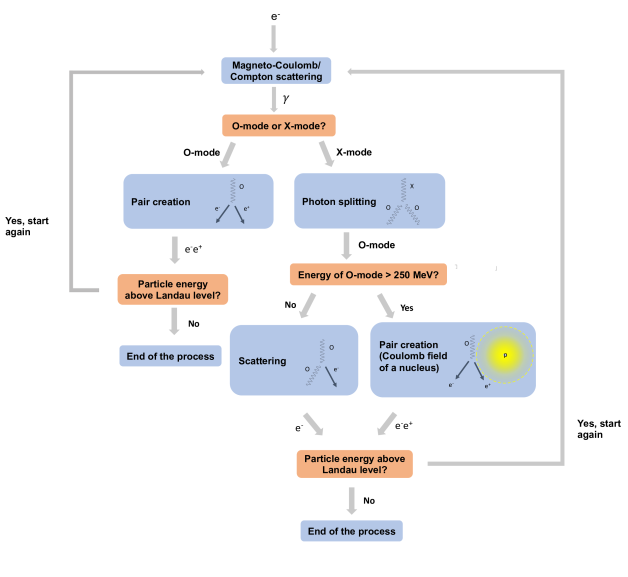
Figure 1: Electron-positron avalanche due to particle bombardment. The figure refers to magnetic field $B\sim 10^{15}$ G, in which case, after the initial Magneto-Coulomb or Compton scattering interaction most of the energy is transferred to photons (either O- or X-mode) and the electron retains a limited fraction of its kinetic energy. The long, right hand side branch that departs after the Magneto-Coulomb/Compton Scattering interaction describes the different mechanisms triggered by the initial penetration of a X-mode photon (under the assumption that O-mode photons resulting from the photon splitting have energy below the threshold for direct pair creation). In this branch, after a scattering, the O-mode photon transfer most of its energy to an electron. See text for details

As discussed by Lyubarsky & Eichler (2007), during collisional Landau level excitations most of the energy is transferred to photons (the seed electrons retain only a small fraction of the total energy). The resulting gamma-rays can trigger an electron-positron pairs avalanche, ultimately leading to electrons with the energy below the Landau energy. If the pair avalanche is triggered by O-mode gamma rays, the typical length scale in which it occurs is roughly coincident with the stopping length of the charged particles and is given by (Lyubarsky & Eichler, 2007)

$$l_{{}_{Low}}\approx\frac{2B}{3\xi B_{q}Z^{2}n_{i}\sigma_{T}}\ln\left[\ln\left(\frac{0.4\gamma^{2}B_{q}}{B}\right)\right]\,,$$ (2)

where $\xi\approx 0.15(B/10^{15}~{}\rm{G})^{-1/2}$ is the fraction of the kinetic energy retained by the electron after one scattering, $B_{q}=m_{e}c^{3}/\hbar e=4.4\times 10^{13}$ G is the critical quantum field, $Z$ is the atomic number, $\sigma_{T}$ is the Thomson cross section, and $n_{i}$ is the number density of ions. For $\gamma\sim 100-1000$, this translates into a Thomson depth of

$$\tau_{0}=\sigma_{T}Znl_{Low}\approx 200Z^{-1}\left(\frac{B}{10^{15}\,{\rm G}}\right)^{3/2}\,.$$ (3)

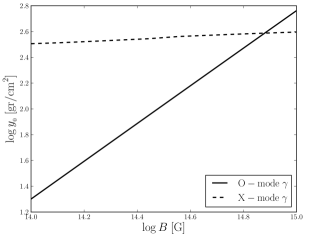
Figure 2: Stopping column density for different magnetic fields. The solid line shows the penetration length of the electron-positron avalanche produced by the initial O-mode photon branch (after a magneto-Coulomb interaction for particles with Lorentz factor $\gamma=10^{3}$). The dashed line shows the penetration of the electron-positron avalanche due to X-mode photons.

X-mode gamma rays do not produce pairs directly but they first split into O-mode photons (see the right hand side branch after the initial Magneto-Coulomb interaction in Figure 1). If the energy of the resulting O-mode photon is below the energy threshold for direct pair creation then a) pairs may be created via the interaction with the Coulomb field of a nucleus or b) the O-mode photon may transfer the energy to an electron via Compton scattering, which then may undergo a Magneto-Coulomb interaction. Lyubarsky & Eichler (2007) calculated the mean free path for successive production of X-mode photons for particles with Lorentz factor $\gamma=10^{3}$, moving in a magnetic field of $B=10^{15}$ G, finding that the avalanche can extend up to a relatively large optical depth

$$\tau_{0}\approx 300Z^{-1}.$$ (4)

In a hydrogen atmosphere, this translates into a relatively large column density for stopping the successive production of X-mode photons $y_{{}_{0}}\sim 750~{}\rm{g~{}cm}^{-2}$, while seed electrons from the particle bombardment are stopped at $y_{{}_{0}}\sim 570~{}\rm{g~{}cm}^{-2}$. However, by repeating the same calculations for a magnetic field $B=10^{14}$ G, we found that the stopping column density can be reduce to $y_{0}\sim 250~{}\rm{gr~{}cm}^{-2}$ for X-ray photons, and to $y_{0}\sim 20~{}\rm{gr~{}cm}^{-2}$ for seed electrons. It should be noticed that, in the case in which the energy of the O-mode photon is above the threshold for direct pair creation, the pair avalanche penetrates the atmosphere up to a depth significantly less than that of equation (3). The stopping column densities for different magnetic fields for both the X-mode and O-mode branches are also shown in Figure 2.

In a “high” density plasma, i.e. such that $c\sigma_{01}n\gg 1/(\gamma\tau)$, the impinging charged particles can be excited, via successive scatterings, to Landau levels with large quantum numbers (Kotov et al., 1986). In this case, the electron mean free path has been calculated by Kotov et al. (1986), and is given by

$$l_{{}_{High}}=2.35\times 10^{8}\frac{B_{q}}{ZB}\left(\frac{\xi}{n\Lambda}\right)^{1/2},$$ (5)

where $\Lambda$ is the Coulomb logarithm.

Potekhin (2014) compared this result with the geometrical depth obtained from the NS envelope models of Ventura & Potekhin (2001) and performed a numerical fit to find a simple analytic formula for the column density at which particles decelerate. Assuming that $\Lambda=1$, this column density is given by

$$y_{{}_{0},High}\approx\left[\left(\frac{A}{Z^{2}}\frac{\gamma}{700}\right)\left(\frac{B}{10^{12}~{}\rm{G}}\right)^{-2}\right]^{0.43}\left(\frac{T}{10^{6}\rm{K}}\right)~{}\rm{g~{}cm}^{-2},$$ (6)

where $T$ is the temperature of the atmosphere, which enters in the expression of the stopping length because a definite atmospheric model was used. It should be noticed that Eq. (6) scales with the magnetic field as $\propto B^{-0.86}$, which means that for stronger magnetic fields the column density decreases, as well as the density at which particles lose most of their kinetic energy. Then, for strong magnetic fields, large Lorentz factors are required in Eq. (6) to satisfy the criterion of high density plasma. It is worth noticing also that, since the low stopping length inferred by Eq. (6) have been invoked to suggest the existence of a self-regulating mechanism driven by magnetospheric currents which may produce thin hydrogen layers on the surface of ultra magnetized NSs (Ho et al., 2007; Potekhin, 2014), the existence of such ultra-relativistic particles ($\gamma\sim 10^{14}$ for $B\sim 10^{13}$ G) is necessary in order to make the scenario self–consistent.

In a twisted magnetosphere, particles are accelerated to typical Lorentz factor $\gamma\sim 10^{3}-10^{6}$. Assuming $\gamma=10^{3}$, and considering magnetic fields $B\sim 10^{14}$ G, the cross section to excite particles to the first Landau level is $\sigma_{01}\sim 10^{-25}~{}\rm{cm}^{2}$ (assuming $\Lambda=1$), and the typical life-time of the process is $\tau\sim 10^{-19}~{}\rm{s}$ (Kotov & Kelner, 1985). This means that the condition of low density plasma (Eq.1) requires $n\ll 10^{29}~{}\rm{cm}^{-3}$, which is typically met across the NS atmosphere. Thus, in the following, only the stopping length corresponding to the low density case is considered. We should notice that the estimates for the stopping optical depth, eqs. (3) and (4) are based on cross sections for magneto-Coulomb interactions, photon splitting induced by the the magnetic field (or the Coulomb field of a nucleus), and Compton scattering processes (Klein-Nishina cross section) that are not accounting for all the complex physics of plasma in super strong magnetic fields. Detailed calculations for these processes in the magnetar regime are outside the scope of this study. However, we can conclude that by considering a range of stopping column densities as large as $y_{{}_{0}}\approx 50-500~{}\rm{g~{}cm}^{-2}$, gives scenarios fairly compatible with values previously discussed for particles decelerated in a low density plasma, inasmuch the lower limit is representative of the penetration of the particle bombardment for magnetic fields $B\sim 10^{14}$ G, while the upper limit is representative of the penetration of successive X-mode photons production for $B\sim 10^{15}$ G. Both cases assume initial particle bombardment with Lorentz factor $\gamma=10^{3}$.

Another important process that can contribute to the stopping length is resonant Compton drag. In fact, upon impinging on the atmosphere, electrons feel a hot photon bath (with typical temperature of $T\sim 10^{7}$ K, see next sections) and, in presence of a high magnetic field, may undergo significant resonant Compton cooling. This process has been investigated by Daugherty & Harding (1989), Sturner et al. (1995) and, more recently, by Baring et al. (2011) who calculated the electron cooling rate using the fully relativistic, quantum magnetic Compton cross section. As shown by Baring et al. (2011, see their Fig. 6), the electron cooling length scale varies considerably with both, the Lorentz factor of the charges and the photon temperature and reaches a minimum at the onset of the resonant contribution, in correspondence of $\gamma_{r}\approx B/(\Theta B_{q})$, where $\Theta=kT/m_{e}c^{2}$. They found that, for $B\gg B_{q}$, the absolute minimum of the Compton stopping length is

$$\lambda_{C}\sim\frac{2\tilde{\lambda}B}{B_{q}\alpha_{F}\Theta^{3}}\,,$$ (7)

where $\tilde{\lambda}$ is the reduced electron Compton wavelength, and $\alpha_{F}$ the fine structure constant. The previous expression strongly depends on the temperature.

For $B=10^{14}$ G and $T=10^{7}$ K, this gives $\lambda_{C}\sim 100~{}\mathrm{cm}$, in correspondence of a Lorentz factor $\gamma\sim 10^{3}$. In turns, assuming a density $\rho\sim 10^{-3}~{}\mathrm{g~{}cm}^{-3}$, this translates into a stopping column density as small as $y_{0}\sim 0.1~{}\mathrm{g~{}cm}^{-2}$. Indeed, by assuming that the Compton stopping length grows linearly with $\gamma$ for $\gamma>\gamma_{r}$ (see the curves in Fig. 6 of Baring et al., 2011), we can estimate that the Compton stopping length becomes larger than the stopping length for magneto-Coulomb collisions (so the latter effect becomes dominant) only if the charge Lorentz factor is $\gamma>10^{6}$.

On the other hand, even considering $\gamma\sim 10^{3}$, we stress that an expected value $y_{0}\sim 0.1~{}\mathrm{g~{}cm}^{-2}$ is an absolute lower limit, for several reasons. First, it assumes monoenergetic particles at $\gamma_{r}$. As soon as the Lorentz factor departs from this value, the resonant process becomes more inefficient and the Compton stopping length increases (extremely rapidly at lower $\gamma$, and almost linearly for $\gamma>\gamma_{r}$). Moreover, this value is estimated assuming that the radiation field is isotropic (while this is not expected to be the case in the external layers of our magnetized atmospheres) and the resonant conditions (which is in general angle-dependent) is met by all impinging charges.

In any case, while experiencing Compton drag, the cooling electrons produce hard X-ray/soft gamma-ray photons, primarily but not exclusively in the X mode (Beloborodov, 2013; Wadiasingh et al., 2018), and these X-mode photons can split into O-mode photons, which can produce a pair cascade, contributing to the process previously described (see discussion after Eq. 3). In order to estimate the stopping length at which the pair cascade (and heat deposition) end, we can then repeat the same calculation as before, by using again a magnetic field $B=10^{14}$ G. If we assume that a seed electron (stopped at $y_{0}=0.1~{}\mathrm{g~{}cm}^{-2}$) with Lorentz factor $\gamma=10^{3}$ transfers all the energy, or 1/2 of the energy, or 1/4 of the energy to a single X-mode photon, then the results is similar to what discussed before, i.e. the e⁺e^- cascade stops at $y_{0}=326~{}\mathrm{g~{}cm}^{-2}$, $y_{0}=321~{}\mathrm{g~{}cm}^{-2}$ or $y_{0}=187~{}\mathrm{g~{}cm}^{-2}$, respectively. This is because, during the cascade, the stopping column density is dominated by the characteristic length travelled by O-mode photons (produced by splitting of X-mode photons) before producing pairs, rather than the path travelled by the pairs themselves (which can be effectively stopped by resonant Compton drag at the site of creation).

In the following, we will carry on the analysis by considering a range of stopping column densities $y_{{}_{0}}\approx 65-500~{}\rm{g~{}cm}^{-2}$, which covers the scenarios described before for charges with impinging Lorentz factor $\sim 10^{3}$. In this range of values, we ensure a convergence of our numerical code. The potential effects of a larger Lorentz factor are briefly discussed in the conclusions and summary section.

For simplicity, we assume that the heat deposition is distributed uniformly along this depth, and is given by

$$W_{{}_{H}}=L_{\infty}/4\pi R^{2}y_{{}_{0}}$$ (8)

where $L_{\infty}$ is the luminosity at infinity and $R$ is the star radius. This expression is valid as long as the velocity, $v$, of incoming magnetospheric particles is much higher than the thermal velocity of the plasma, $v_{th}$, which allows us to ignore collective plasma oscillation (Alme & Wilson, 1973; Bildsten et al., 1992). We assume that the only heating source in the atmosphere is due to the particle bombardment, which means we set $W_{H}=0$ for $y>y_{{}_{0}}$.

2.2 Radiative transfer

In the following we compute the transport of radiation in magnetized atmospheres heated by particles bombardment induced by a twisted magnetosphere. According to Beloborodov & Thompson (2007), the twist current $\boldsymbol{j}=(c/4\pi)\nabla\times\boldsymbol{B}$ is maintained by a voltage $\Phi$ that is regulated by a $e^{+}e^{-}$ discharge along the magnetic field lines. For a non-rotating NS with a twisted dipole, as the magnetosphere untwist, the cavity in which $\nabla\times\boldsymbol{B}=0$ expands out from the equatorial plane, and the currents become concentrated in a “j-bundle” which footprints are anchored near the magnetic poles. The evolution of the j-bundle, where the back bombarding currents are accelerated, produces a polar hot spot that shrinks over time. The luminosity associated to currents returning onto the NS surface is given by (Beloborodov, 2009).

$$L\approx 1.3\times 10^{36}B_{14}R_{6}\psi{\cal V}_{9}u_{\star}^{2}~{}\rm{erg~{}s}^{-1},$$ (9)

where $\psi$ is twist angle, ${\cal V}_{9}$ is a threshold voltage in units of $10^{9}$ V, and

$$u_{\star}(t)\approx\frac{cR{\cal V}}{2\mu\psi}(t_{end}-t)$$ (10)

defines the (time dependent) magnetic flux surface in which is located the current front (or sharp boundary of the cavity), with $t_{end}=\mu\psi_{{}_{0}}/cR{\cal V}$ the time required to erase the twist. Here, $\psi_{{}_{0}}$ is the amplitude if the twist imparted by the starquake and $\mu$ is the magnetic dipole moment. Owing to the gravitational redshift, the total luminosity seen by a distant observer, $L_{\infty}$, is related to the local luminosity at the top of the atmosphere by $L_{\infty}=y_{{}_{G}}^{2}L(0)$, where $y_{{}_{G}}=(1-R/R_{s})^{1/2}$ is the gravitational redshift factor in a Schwarzschild spacetime for a star with radius $R$ and Schwarzschild radius $R_{s}$.

The envelope material is assumed to be pure, completely ionized hydrogen. In order to solve the energy balance and radiative transfer, we work in plane-parallel approximation and we compute equilibrium solutions in the frequency-integrated case. We follow the same approach that has been used by Turolla et al. (1994), Zampieri et al. (1995), and Zane et al. (2000) for computing model atmospheres at low accretion rates in the non-magnetized and moderately magnetized regime (see also Zel’dovich & Shakura, 1969; Alme & Wilson, 1973, for earlier works). The structure of the atmosphere is obtained by solving the hydrostatic equilibrium equation

$$\frac{\mathrm{d}P}{\mathrm{d}y}=\frac{GM}{y_{{}_{G}}^{2}R^{2}},$$ (11)

where $G$ is the gravitational constant, $M$ is the mass of the star and $P=k\rho T/\mu_{e}m_{p}$ is the gas pressure, with $T$ the gas temperature and $\mu_{e}=1/2$ (for fully ionized hydrogen). Eq. (11) can be solved analytically, giving the density as a function of the column density

$$\rho=\frac{GMm_{p}}{2y_{{}_{G}}^{2}R^{2}}\frac{y}{kT(y)}\,.$$ (12)

We are interested in luminosities typical of magnetar sources, $L=10^{34}-10^{36}~{}\rm{erg~{}s}^{-1}$, in which case both, the ram pressure by the particle bombardment and the radiative force are negligible with respect to the thermal pressure and the gravitational force, respectively.

The differential equation for the total luminosity is given by (Zampieri et al., 1995)

$$\frac{1}{4\pi R^{2}}\frac{\mathrm{d}L}{\mathrm{d}y}=-\frac{W_{H}}{y_{{}_{G}}},$$ (13)

which can be combined with Eq. (8) to derive an analytical solution for the luminosity,

$$L(y)= \frac{L_{\infty}}{y_{{}_{G}}}\frac{y_{{}_{0}}-y}{y_{{}_{0}}} y<y_{0}$$ (14)

$$L(y)= 0 y\geqslant y_{{}_{0}}$$

In a magnetized plasma, the polarized radiative transfer problem can be described by a system of two coupled differential equations for the specific intensities of ordinary and extraordinary photons. In the Eddington and plane-parallel approximation, the first and second moments of the radiative transfer equations can be written in terms of the luminosity, $L_{i}$, and radiation energy density, $U_{i}$, of each normal mode (with $i=1,2$), both measured by the local observer, as

$$\frac{1}{4\pi cR^{2}}\frac{\mathrm{d}L_{i}}{\mathrm{d}y} = \kappa^{P}_{i}\left(\frac{aT^{4}}{2}-U_{i}\right)+\bar{S}(U_{3-i}-U_{i}),$$ (15)

$$\frac{1}{3}\frac{\mathrm{d}U_{i}}{\mathrm{d}y} = \kappa^{{}_{R}}_{i}\frac{L_{i}}{4\pi R^{2}cy_{{}_{G}}},$$ (16)

where $\bar{S}$ is the scattering mean opacity from one normal mode to the other, and $\kappa_{i}^{P}$ and $\kappa_{i}^{{}_{R}}$ correspond to the Planck and Rosseland mean opacity for each normal mode, respectively. In absence of a complete frequency-dependent calculation (which is outside the purpose of this paper), we approximated the absorption mean opacity and the flux mean opacity with $\kappa_{i}^{P}$a and $\kappa_{i}^{{}_{R}}$, respectively, for each mode of propagation.

In the following, we neglect collective plasma effects and consider only the limit $\omega_{p}^{2}/\omega^{2}\ll 1$, where $\omega_{p}$ is the plasma frequency. We also consider only frequencies lower than the electron cyclotron frequency, so the semitransverse approximation can be assumed to hold. With the exclusion of the very external layers, the temperature in the atmosphere is always lower than $\sim 10^{7}$ K, so that scattering dominates over true absorption only for $\tau\sim 1$ and Comptonization is negligible. For this reason, similarly to what has been done in the previous investigations, only conservative scattering is accounted for in the transfer equations. We consider a plasma composed of protons, electrons and we do take into account for vacuum corrections in the polarization eigenmodes, that start to be important when the magnetic field approaches the quantum critical limit, $\sim B_{q}$. These corrections induce the breakdown of the normal mode approximation at the mode collapse points (MCPs), where the two normal modes can cross each other or have a close approach, depending on the photon propagation angle (see Pavlov & Shibanov 1979, Zane et al. 2000. see §2.3). The detailed expressions of the magnetized free free and Thomson scattering opacities are discussed later on, together with the method we followed for their numerical evaluation and average (§ 2.3).

Despite Comptonization is expected to be negligible as far as the radiative transfer equations are concerned, in analogy to the case of accreting atmospheres, we expect that it has an important role in establishing the correct energy balance in the external, optically thin layers (Alme & Wilson, 1973; Turolla et al., 1994; Zampieri et al., 1995; Zane et al., 2000) where the heating deposited by the incoming charges needs to be balanced by Compton cooling. Accordingly, we write the energy balance equation as

$$\frac{\kappa^{P}}{\kappa_{s}}\left(\frac{aT^{4}}{2}-\frac{\kappa^{P}_{1}}{\kappa^{P}}U_{1}-\frac{\kappa_{2}^{P}}{\kappa^{P}}U_{2}\right)+(\Gamma-\Lambda)_{c}=\frac{W_{H}}{c\kappa_{s}}$$ (17)

where $(\Gamma-\Lambda)_{c}$ is the Compton heating-cooling term, evaluated using the approximation of Arons et al. (1987), $\kappa^{s}$ is the total (summed over the two modes) scattering opacity and $\kappa^{P}=\kappa^{P}_{1}+\kappa^{P}_{2}$ is the total Planck mean opacity. One complication is that the Compton heating-cooling term in equation (17) depends on the radiation temperature, $T_{\gamma}$, which in turn should be obtained by solving the frequency-dependent transport of radiation. To overcome this problem, we assume that the energy exchange between photons and the gas particles, due to multiple Compton scatterings, is governed by the equation (Wandel et al., 1984; Park & Ostriker, 1989; Park, 1990; Turolla et al., 1994; Zampieri et al., 1995)

$$\frac{y}{T_{\gamma}}\frac{\mathrm{d}T_{\gamma}}{\mathrm{d}y}=2Y_{c}\left(\frac{T_{\gamma}}{T}-1\right),$$ (18)

where $Y_{c}~{}=~{}(4kT/m_{e}c^{2})\rm{max}(\tau_{es},\tau_{es}^{2})$ is the Comptonization parameter and $\tau_{es}~{}=~{}\kappa_{s}y$ is the scattering optical depth.

The system of differential equations given by equation 15 (solved for mode 1 only, since the luminosity of mode 2 can be then obtained by difference using equation 14 for the total luminosity), equation 16 (solved for both modes) and equation 18 needs to be solved coupled to a set of 4 boundary conditions. First, we assume a non-illuminated atmosphere, which translates into a free streaming condition relating the total energy density of the radiation to the total luminosity, at the outer layer of the atmosphere,

$$U(y_{min})=U_{1}(y_{min})+U_{2}(y_{min})=\frac{L^{\infty}_{1}+L^{\infty}_{2}}{2\pi R^{2}cy_{{}_{G}}},$$

where $y_{min}$ correspond to the minimum value of the column density grid used in the atmosphere model. Second, we assume energy equipartition in the inner, optically thick, atmospheric region, where the energy density of each mode approaches $\sim aT^{4}/2$, and we set $U_{1}(y_{max})=U_{2}(y_{max})$, where $y_{max}$ is the maximum value of the column density grid used in the model calculation. Furthermore, we assume photons in thermodynamic equilibrium with the gas in the inner layers of the atmosphere, therefore the radiation temperature must be equal to the gas temperature $T_{\gamma}(y_{max})=T(y_{max})$. Finally, since the observed luminosity is produced by re-irradiation of the heat deposited by particle bombardment, with $W_{H}=0$ for $y>y_{{}_{0}}$, the condition $L_{1}(y>y_{{}_{0}})=L_{2}(y>y_{{}_{0}})=0$ is used in the inner regions of the atmosphere.

2.3 Opacities

Absorption and scattering opacities in a magnetized medium were widely investigated in the literature (see e.g. Mészáros 1992, Harding & Lai 2006, Potekhin 2014 and references therein). For magnetic fields close to or exceeding the quantum critical field, the contributions of the vacuum to the dielectric and magnetic permeability tensors become important. In particular when the plasma and vacuum contributions balance, a vacuum resonance appears, where mode conversion may occur (Gnedin et al., 1978; Pavlov & Shibanov, 1979; Meszaros & Ventura, 1979).

For $B\leq B_{q}=4.4\times 10^{13}$ G, the vacuum parameter is given by (Gnedin et al. 1978; see also Kaminker et al. 1982)

$$W=\left(\frac{3\times 10^{28}\rm{cm}^{-3}}{n_{e}}\right)\left(\frac{B}{B_{q}}\right)^{4}$$ (19)

where $n_{e}$ is the electron number density.

The ellipticities of the normal modes for electromagnetic waves in the magnetized plasma are obtained from (Kaminker et al., 1982)

$$q=\frac{\sin^{2}\theta}{2\cos\theta}\sqrt{u}\left(1-W\frac{u-1}{u^{2}}\right),$$ (20)

where $u=\omega_{{}_{c,e}}^{2}/\omega^{2}$, $\omega_{{}_{c,e}}=eB/m_{e}c$ is the electron cyclotron frequency and $\theta$ is the angle between the wave propagation direction and the magnetic field. The condition $q=0$ determines the frequencies and photon directions (for each value of density and magnetic field) at which the normal modes approximation breaks downs (due to vacuum corrections and proton resonance). At this MCP a proper treatment of radiative transfer should be performed via the Stokes parameters, while our equations are written assuming that the normal mode approximation holds for all photon propagation directions. Following Pavlov & Shibanov (1979), we estimate the critical angle associated to the normal modes breakdown at the vacuum MCP from the expression

$$\frac{\cos\theta_{n}}{\sin^{2}\theta_{n}}=\pm\frac{1}{2\sqrt{u}}\left[\gamma_{\parallel}(u-1)+\gamma_{\bot}\left(1-\frac{2W}{u}\right)\right]_{q=0},$$ (21)

where $\gamma_{\parallel,\bot}=(\nu_{\parallel,\bot}+\nu_{r})/\omega\sim 10^{-5}-10^{-3}$. Here, $\nu_{r}$ is a radiative width and $\nu_{\parallel,\bot}$ is an effective electron-ion collision frequency (for details see Pavlov & Shibanov 1979). At $\theta_{n}$ the normal modes have maximum non-orthogonality (i.e. maximum coincidence). If $\theta_{n}\to\pi/2$, the interval of non-orthogonality collapses to a point and, for almost all waves (i.e. all those with $\beta=|\pi/2-\theta|>\beta_{n}=|\pi/2-\theta_{n}|$), the polarization ellipses are rotated through $90\deg$ while crossing the resonance (mode switching). Vice versa, if $\theta_{n}$ is small the evolution of the electromagnetic waves across the resonance is not well understood. In the numerical simulation, we then set complete mode conversion at the vacuum resonance as long as $\theta_{n}>50~{}\deg$.

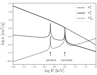
Figure 3: Angle integrated opacities for a fully ionized H atmosphere with magnetic field $B=10^{14}$ G (normal to the surface), temperature $T=10^{7}$ K and density $\rho=10~{}\rm{gr~{}cm}^{-3}$. The dashed and solid lines correspond to the free-free absorption opacities in mode 1 (X-mode) and mode 2 (0-mode), respectively. The dotted line correspond to the scattering opacity from mode 1 to mode 2. Notice that due to opacity symmetry $\kappa^{s}_{12}=\kappa^{s}_{21}$. The arrows indicate the proton and vacuum resonances.

Notice that other important effects under strong magnetic field such as partial ionization or the appearance of additional narrow resonant features due to higher harmonics of the proton cyclotron frequencies may be present (for a review see Potekhin 2014). However, for simplicity they are not considered in the present work, which is anyway restricted to a frequency integrated calculation.

Under the conditions we expect, conservative electron scattering can be safely assumed. The corresponding expressions for the opacity are taken form Ventura (1979) and Kaminker et al. (1982), while those for ions from Pavlov et al. (1995). Opacities for both electrons and ions bremsstrahlung are from Pavlov & Panov (1976), Mészáros (1992) and Pavlov et al. (1995), and we implemented the numerical evaluation of the magnetic Gaunt factors as in Zane et al. (2000).

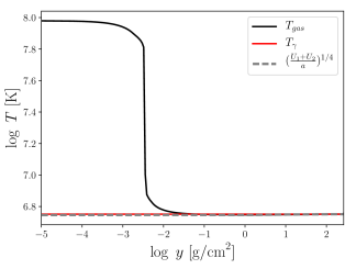
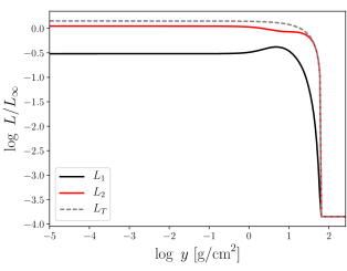
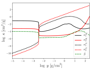
Figure 4: Gray atmosphere solution for total luminosity $L_{\infty}=10^{36}~{}\rm{erg/s}$, stopping column density $y_{{}_{0}}=65~{}\rm{gr/cm}^{2}$ and magnetic field $B=10^{14}~{}\rm{G}$. Top-left panel: gas temperature profile, $T$ (black solid line), and photon temperature profile, $T_{\gamma}$ (red solid line). The temperature associated to the total energy density is shown in the gray dashed line. Top-right panel: energy densities associated to $U_{1}$ (black solid line), $U_{2}$ (red solid line) and $T_{\gamma}$ (dashed gray line) normalized to $U_{\infty}=L_{\infty}/4\pi R^{2}c$. Bottom-left panel: luminosity profiles $L_{1}$ (black solid line) and $L_{2}$ (red solid line). The total (analytical) luminosity $L_{T}$ is shown in the gray dashed line. Bottom-right panel: Planck mean opacities, $\kappa_{1}^{{}_{P}}$ (black dotted line) and $\kappa_{2}^{{}_{P}}$ (red dotted line), and Rosseland mean opacities, $\kappa_{1}^{{}_{R}}$ (black solid line) and $\kappa_{2}^{{}_{R}}$ (red solid line). The scattering mean opacity from mode 1 to mode 2 (and vice versa), $\bar{S}$, is shown in the green dashed line.

Figure 3 shows the energy dependent free-free absorption and the mode exchange scattering opacity used in our calculations. In general, for most energies, opacities are dominated by photon-electron interaction. However, for the magnetic fields that we are considering, $B\sim 10^{14}$ G, protons also play an important role as they produce a sharp feature in the X-mode opacities at the proton cyclotron energy, which lies within the soft X-ray band (see Zane et al. 2001, Ho & Lai 2001 and Özel 2003 for the discussion of the impact of this feature in the emergent spectrum from atmospheres of magnetized NSs). On the other hand, vacuum effects introduce additional features to the opacity profiles. In fact, when complete mode conversion is present, vacuum effects produce a step change in the free-free opacities across the vacuum resonance, due to the exchange of the X-mode opacity with the O-mode opacity (and vice versa; see Ho & Lai 2003 for a discussion of the vacuum resonance with and without mode conversion). Instead, vacuum effects produces a raise (spike feature) in the (angle-integrated) mode exchange scattering opacity at the vacuum resonance.

As mentioned in § 2.2, in our numerical calculation we use the above opacities suitably integrated in frequency in strict analogy with the definition of the absorption mean opacity and the flux mean opacity in the unmagnetized case. A further problem encountered while performing the integration in energy is related to the fact that the vacuum resonance is located at different energies in different layers of the atmosphere. To avoid overestimating the mean opacity due to the finite size of the energy grid, which can lead to numerical problems of convergence in our calculations, we compute the opacity near the vacuum resonance feature at the energy point $E_{v}$ as an average between its values at two adjacent energies $E_{-}=E_{v}-\Delta E_{bin}/3$ and $E_{+}=E_{v}+\Delta E_{bin}/3$. We tested numerically that varying the way in which we chosen the adjacent energies only produces negligible differences in the resulting integral.

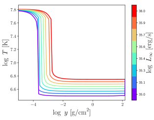
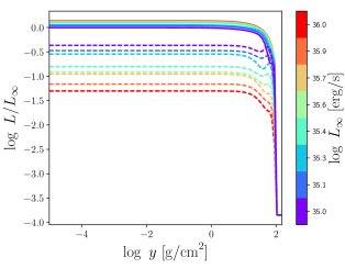
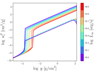
Figure 5: Gray atmosphere solutions for different luminosities (see vertical color bar), fixed magnetic field $B=3\times 10^{14}$ G, and fixed stopping column density $y_{{}_{0}}=100~{}\rm{gr~{}cm}^{-2}$. The temperature profile for the atmospheric plasma is shown in the top-left panel. The luminosity $L_{1}$ (top-right panel), Planck mean opacity $\kappa_{1}^{{}_{P}}$ (bottom-left panel), and Rosseland mean opacity $\kappa_{1}^{{}_{R}}$ (bottom right panel) are shown by dashed lines. Similarly, the corresponding profiles for $L_{2}$, $\kappa_{2}^{{}_{P}}$, and $\kappa_{2}^{{}_{R}}$ are shown by solid lines.

3 Numerical solutions

The numerical calculation was performed by readapting the code presented by Turolla et al. (1994), which was meant for unmagnetized atmospheres under accretion, to the case of magnetized NS atmospheres heated by particle bombardment. We started from the numerical routines for the opacities from Zane et al. (2000) and created all necessary routines for the computation of the energy integrated opacities required by this work (see previous section). Solutions are then found using a numerical iterative scheme. First, an initial temperature profile is specified, taking as trial solution the temperature profile of a non-magnetized atmosphere from Turolla et al. (1994). This, together with eq. (12) sets also the initial density profile. Then, we solve the transport of radiation via eqs. (15), (16) and (18) to obtain the profiles for $L_{i}$, $U_{i}$ and $T_{\gamma}$. These, in turn, are used to compute a new temperature profile, that satisfies the energy balance, eq. (17). The procedure is iterated until the relative difference between two successive solutions is $<10^{-5}$, in each variable. Convergence is typically reached after $\sim 15$ iterations.

In all models, a NS with mass $M=1M_{\odot}$ and radius $R=10$ km is assumed. Solutions are computed by using a logarithmic grid of 100 equally spaced points for the column density $y$ in the range $[10^{-5}-10^{2}]~{}\rm{gr~{}cm}^{-2}$. We report the models for magnetic field values $B\approx 10^{14}-10^{15}$ G and luminosities $L_{\infty}\approx 10^{35}-10^{36}~{}\rm{erg~{}s}^{-1}$, which are characteristics of the brightest magnetars, and stopping lengths in the range $y_{0}=65-500~{}\rm{gr~{}cm}^{-2}$ (see § 2.1).

3.1 Results

Fig. 4 shows the temperature, energy density, luminosity and opacity profiles for a NS atmosphere with $B=10^{14}$ G, stopping length $y_{0}=65~{}\rm{gr~{}cm}^{-2}$ and total luminosity $L_{\infty}=10^{36}~{}\rm{erg~{}s}^{-1}$. The temperature profile (top-left panel) shows the formation of a hot layer in the most external part of the atmosphere. This external temperature profile is similar to those obtained in the case of atmospheres of NS accreting at low rate from the interstellar medium (see Turolla et al. 1994 and Zane et al. 2000). As discussed in previous works, free-free cooling is not effective in balancing the heating (in this case caused by the particle bombardment) in this region. As a consequence, the plasma temperature raises until a point in which Compton cooling becomes efficient (see Zane et al. 2000 and references therein). Since the radiation is produced only by the particle bombardment (or, alternatively, the luminosity by particle bombardment is much larger than the NS cooling luminosity), in the deepest layers the luminosity vanishes and the temperature profile becomes constant. The radiation temperature shows that most of the radiation decouples from the plasma in the internal region of the atmosphere, before photons start travelling across the hot external layer.

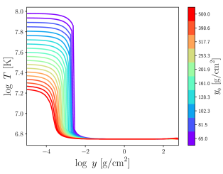
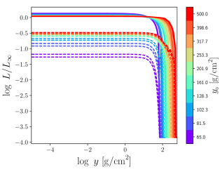
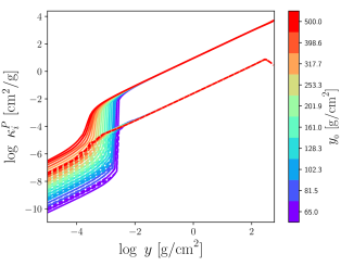
Figure 6: Same as Fig. 5, but varying the stopping column density $y_{{}_{0}}$. Here, the total luminosity is set to $L_{\infty}=10^{36}~{}\rm{erg/s}$ and the magnetic field to $B=4\times 10^{14}$ G.

The top-right and bottom-left panels of Fig. 4 show the energy density and the luminosity of the two modes. Clearly, $U_{i}$ is constant in the internal layers where the luminosity vanishes and energy equipartition is reached between the two radiation modes. As matter and radiation start decoupling, most of the luminosity is produced in an internal region, characterized by a substantial and non vanishing energy density gradient, $\mathrm{d}U_{i}/\mathrm{d}y$, in which diffusion approximation holds. It is interesting to notice how the energy density profiles cross, at some point within the atmosphere, reflecting the mode conversion due to vacuum effects (Fig. 4, bottom-right panel). This is an interesting effect since it can impact on the expectations for the polarization signal. In fact, since the plasma is highly magnetized, the emerging radiation is expected to be highly polarized, in principle even up to 100$\%$: the large difference in the plasma opacities of the two modes implies that most of the radiation should be carried by the mode for which the atmosphere is more transparent (see for example Özel 2001 and Ho & Lai 2003 for a discussion in the context of atmosphere for passively cooling NSs). However, vacuum mode conversion partly reduces the difference in the opacities, and therefore in luminosity, of the two modes, potentially reducing the polarization signal. If an “intrinsic” polarization fraction is defined as $PF=(L_{\infty,1}-L_{\infty,2})/(L_{\infty,1}+L_{\infty,2})$, then $PF\approx 0.6$ in the model at hand.

In the following, we explore the numerical solutions for different values of luminosity, stopping length and magnetic field. In order to isolate the effects of each parameter, we vary one of these quantities at each time, keeping fixed the other model parameters. We present the profiles for temperature, luminosity, Planck and Rosseland mean opacities as they are the most relevant to discuss the behaviour of the solution (the scattering opacity is in fact negligible in most of the atmosphere).

3.1.1 Models with different luminosity

Fig. 5 shows a set of solutions computed for $y_{{}_{0}}=100~{}\rm{gr~{}cm}^{-2}$, $B=3\times 10^{14}$ G, and by varying the total luminosity in the range $L_{\infty}=10^{35}-10^{36}~{}\rm{erg~{}s}^{-1}$. As expected, higher luminosities, which are related to larger energy deposition in the atmosphere, correspond to hotter atmospheres. Moreover, by increasing the luminosity, the hot atmospheric layer extends inwards, to higher column densities. Luminosity and temperature profiles scale in a roughly self–similar way. However, the expected emergent polarization increases for higher luminosities. This can be understood noticing that, in the inner regions where most of the luminosity is created, the difference between the Rosseland mean opacities associated to each normal mode (lower right panel), is larger for higher luminosities. In diffusion approximation, this translates in a larger suppression of the radiation carried by a mode with respect to the other, and the difference in luminosity then propagates till the top of the atmosphere. For the models presented here, the resulting emergent polarization varies between $0.4<PF<0.9$ for the range of luminosities $L_{\infty}$ considered.

The behaviour for the opacities in these models can be understood as follows. The Planck mean opacity, $\kappa^{{}_{P}}_{i}$, is obtained by performing an integration over energies of the free-free absorption opacity weighted by a blackbody. In turn, the integrand over energy is dominated by the contribution of the free-free opacities at relatively low energies, which are less sensitive to the presence of the vacuum resonance and subsequent mode switching. It follows that, for a fixed magnetic field, the integrand in the opacity scales approximatively as $\kappa^{\rm{ff}}_{i}\propto yT^{-7/2}f_{i}(E)$, where $f_{i}(E)$ is a function of the energy. Since most of the atmosphere has a uniform temperature, this translates into a Planck mean opacity with a linear dependency on $y$. In the external hot layer the temperature increases, and this produces the observed drop in the Planck mean opacities according to the $T^{-7/2}$ dependency of the free-free opacity.

The Rosseland mean opacities, instead, are computed considering the contribution of both, the free-free and scattering opacities. In particular, scattering opacities are dominant at low densities, which is reflected on fact that, in the most external atmospheric layers, the Rosseland mean opacity tends toward a constant. Instead, the free-free opacity is dominant at high densities. Moreover, since in the Rosseland mean opacity the associated integration is performed over the inverse of the energy-dependent opacity, the major contribution from free-free opacities is from the higher energies which are more sensitive to the vacuum resonance. This in turn introduces an additional density dependency, which is reflected in the non linear growth of the Rosseland means at large $y$.

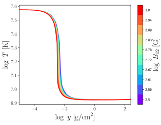
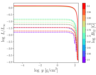
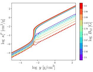
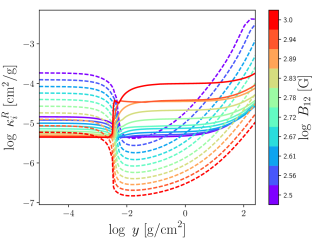
Figure 7: Same as Fig. 5, but varying the magnetic field. Here, the total luminosity is set to $L_{\infty}=5\times 10^{36}~{}\rm{erg/s}$ and the stopping column density to $y_{{}_{0}}=200~{}\rm{gr/cm}^{2}$.

3.1.2 Models with different stopping column density

Fig. 6 shows the solutions for stopping column densities in the range $y_{{}_{0}}=50-500~{}\rm{gr~{}cm}^{-2}$, total luminosity $L_{\infty}=10^{36}~{}\rm{erg~{}s}^{-1}$, and magnetic field $B=4\times 10^{14}$ G. At variance with the models in Sec. 3.1.1, the stopping column density $y_{{}_{0}}$ is anticorrelated with temperature of the hot external layer. Indeed, for smaller stopping column densities, the energy deposition is distributed in a smaller region (see eq. 2.1), which leads to external layers with higher temperatures, as shown in the top-left panel. In this case, the hot layer moves inwards as $y_{{}_{0}}$ decreases. In addition, the most internal layers of the atmosphere have the same temperature for different $y_{{}_{0}}$. This is interesting for future frequency-dependent calculations since it indicates that the typical photon energy deep in the atmosphere is quite insensitive to variations of $y_{{}_{0}}$. Therefore, the spectrum produced in the atmosphere interior may be determined only by the total luminosity and magnetic field strength.

The luminosity carried by each normal mode is shown in the right upper panel of Fig. 6. Similar to the solutions for the temperature profile, the polarization is also anticorrelated with the stopping column density. At variance with models presented in Sec. 3.1.1, the region where the difference in the Rosseland mean opacities of the two modes, $\kappa_{1}^{{}_{R}}$ and $\kappa_{2}^{{}_{R}}$, leads to a larger polarization, is now located in the most external layers of the atmosphere.

As we can see from the left top panel, in the models presented in this section the only change between the solutions is in the temperature (and location) of the external hot layer, while the density profile and the magnetic field are the same for the different models. Accordingly, the strong dependency on $T^{-7/2}$ of the free-free absorption introduces the drop and dispersion between the various curves of the Planck mean opacities seen in the most external atmospheric layers.

The corresponding dispersion in the values of the Rosseland mean opacities at low $y$ (scattering dominated) is instead due to the fact that they are evaluated by convolving the energy-dependent opacity over the derivative of the blackbody, $\mathrm{d}B_{E}(T)/\mathrm{d}T$, calculated at the local value of $T$. For higher temperatures, the peak of this function is located at higher energies. In other words, if the photon bath in the external layer is hotter, then the major contribution to the averaged Rosseland opacity is due to scattering of photons with higher frequency (which in turn may also be more largely affected by vacuum effects).

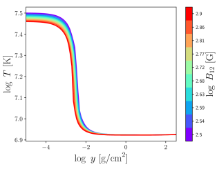
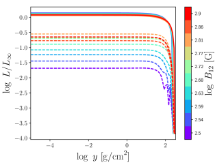
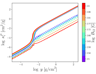
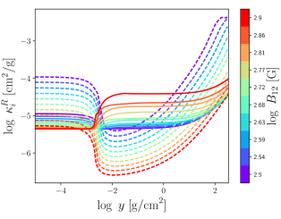
Figure 8: Same as Fig. 5, but varying the magnetic field (vertical color bar) and the stopping column density (see Sec. 3.1.4 for details). Here, the total luminosity is set to $L_{\infty}=5\times 10^{36}~{}\rm{erg/s}$.

3.1.3 Models with different magnetic field

Fig. 7 shows the solutions for magnetic fields in the range $B=3\times 10^{14}-10^{15}$ G, stopping column density $y_{{}_{0}}=200~{}\rm{gr~{}cm}^{-2}$, and total luminosity $L=5\times 10^{36}~{}\rm{erg~{}cm}^{-3}$. As shown in the top-left panel, by varying the magnetic field, and thus the opacities, no significant changes are produced in the temperature profile. Therefore, this suggests that the temperature profile is, instead, determined just by the total luminosity and stopping column density, as discussed in the previous section (Sec. 3.1.2).

The right lower panel shows how the variation of the magnetic fields introduces significant differences in the Rosseland mean opacities $\kappa_{1}^{{}_{R}}$ and $\kappa_{2}^{{}_{R}}$. However, for these opacities, the polarization does not change monotonically with the magnetic field. Instead, the polarization increases as the solutions approach to both the lower and upper end range of the magnetic field considered.

The behaviour of the mean opacities is now much more complicated. By increasing the magnetic field, the X-mode opacities decrease because of the X-mode-reduction factor $\sim 1/(\omega^{2}_{c,e}\omega)$ and $\sim(\omega/\omega_{c,e})^{2}$ present in the free-free and scattering opacities, respectively. However, it should be noticed that by varying the magnetic field also changes the energy associated to the mode switch at the vacuum resonance and its location in the atmosphere. This effect is responsible for a) the fact that the curves of the various Planck mean opacities become closer to each other in the external atmospheric layers and b) the different location of the crossing points of the Rosseland mean opacities (for the two modes) in different models.

3.1.4 Models with different magnetic field and different stopping length

We want to test a scenario in which, as expected, the stopping column density depends on the magnetic field. We describe this dependency in a logarithmic scale as $\log y_{{}_{0}}=-8.7+0.75\log B$ (in cgs units), fairly compatible with the mechanisms discussed (in Sec. 2.1) for decelerating fast magnetospheric particles (with Lorentz factor $\gamma=10^{3}$). We stress that the length scale at which the pair cascade propagates (produced from X-mode photons) is, for these values of parameters, roughly independent on whether the bombarding charge is stopped by a Magneto-Coulomb interaction or by Compton drag. The models are run for a total luminosity $L_{\infty}=5\times 10^{36}~{}\rm{erg~{}s}^{-1}$, a value that is more convenient to ensure numerical convergence. In addition, we also found that it is numerically convenient to solve the the transport of radiation for luminosity in mode 2 (see eq. 14). For doing that, the modes in the Rosseland and Planck mean opacities are flip as $\kappa_{i}^{{}_{R}}\rightarrow\kappa_{3-i}^{{}_{R}}$ and $\kappa_{i}^{P}\rightarrow\kappa_{3-i}^{P}$ (with $i=1,2$), respectively, in the numerical routines that perform their calculations. Notice that there is no need to perform this operation in the mode exchange scattering opacity as $\kappa_{12}=\kappa_{21}$.

Figure 8, top-left panel, shows the solution for the temperature profile. Since lower magnetic fields produce smaller stopping column densities, consequently, the temperature of the external layer increases for lower magnetic fields (as the results discussed in Sec. 3.1.2). By varying the luminosity this trend, qualitatively, still holds (although no quantitative solutions are shown, since, at column densities just below $\sim y_{{}_{0}}$, numerical oscillations start to grow in the region with the steep luminosity gradient).

The solutions for the luminosities in each normal mode, top-right panel, show that the polarization decreases almost monotonically with the magnetic field (except at the upper end of the magnetic field range). This is at variance with the results shown in the Sec. 3.1.3, and it shows that that the polarized signal is affected more strongly by the magnetic field effects on the stopping column density rather than those on the opacities.

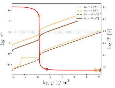
Figure 9: Optical depth as a function of column density for photons in the optical ($E=1$ eV) and ultraviolet band ($E=10$ eV). The model is computed for $L_{\infty}=10^{36}~{}\rm{erg/s}$, $y_{{}_{0}}=100~{}\rm{gr/cm}^{2}$ and $B=4\times 10^{14}$ G. Solid and dashed lines correspond to O-mode and X-mode photons, respectively. The temperature profile is shown by the red solid line (the temperature scale is on the right-hand side). The yellow (brown) circle and yellow (brown) star show the location of the radiation-atmosphere decoupling, $\tau\sim 1$, for O-mode and X-mode photons in the optical (ultraviolet) band, respectively.

3.1.5 Spectral expectations

Some information about the spectral properties of the emerging radiation can be obtained even in the gray model looking at the depth at which photons of different energies decouple. In particular, we compute the energy dependent optical depth (for optical and soft X-rays photons) as

$$\tau_{{}_{E}}^{{}_{i}}=\int_{y_{min}}^{y}\kappa_{{}_{E}}^{a,i}\rm{d}y\prime\,,$$ (22)

where $\kappa_{{}_{E}}^{a,i}$ (with $i=1,2$) is the energy dependent, angle integrated absorption opacity (using $\tau_{{}_{E}}^{{}_{i}}=0$ at $y=y_{min}$).

Figure 9 shows the location of the photon decoupling for the two normal modes. In particular, for O-mode photons with energy $E=1$ eV, i.e. in the optical band, we can see that they decouple in the region of the hot layer. This suggest that the spectrum in the optical, and potentially also in the infrared, may have a flux excess due to the radiation from this hot layer. Instead, X-mode photons with energy $E=10$ eV (in the ultraviolet band), as well as photons with higher energies (in both normal modes) decouple deeper in the atmosphere. These photons are produced in regions with lower and nearly uniform temperature, and so their spectrum may be potentially described by a single black body. These results suggest that the spectrum from a magnetized atmosphere heated by a particle bombardment (single black body with optical/infrared excess), may show substantial deviations from those produced by passively cooling neutron stars (spectrum harder than a blackbody). Models accounting for the full frequency transport of radiation are definitely required to assess this issue and will be the focus of future work.

4 Summary and conclusions

We have presented numerical models for gray atmospheres of magnetized NSs heated by particle bombardment. We assumed a pure, fully ionized hydrogen composition and accounted for the polarized transport of radiation induced by the strong magnetic field. Our main results can be summarized as follows.

• A hot layer is created in the most external region of the atmosphere ($T\sim 10^{8}$ K), similar to what it has been found in previous studies of atmospheres heated by accretion (Turolla et al., 1994; Zane et al., 2000). We found that, in the case presented here, the spatial extent of the layer is primary determined by the luminosity and the stopping column density for the particle bombardment. If there is no significant contribution from the NS cooling (i.e. the luminosity vanishes in the internal layer, as assumed here) then the internal regions of the atmosphere are characterized by a lower (below $T\sim 10^{7}$ K), uniform temperature that is primary determined by the total model luminosity.

• As a consequence, we expect that in the range of frequencies that decouple in the deeper atmospheric layers (e.g. above $\sim 10$ eV) the emergent spectrum may be well approximated by a single blackbody. Instead, photons that decouple in the hot layer (below $\sim 1$ eV) may produce an optical/infrared flux excess, significantly above the extrapolation of the blackbody spectrum coming from the atmosphere interior (see Zane et al. 2000 for similar discussions).

• The expected degree of linear polarization in the emergent spectrum is correlated with the luminosity and anticorrelated with the stopping column density (and almost similarly with the magnetic field, see text for details). Depending on these parameters, the expected intrinsic linear polarization, defined here as $PF=(L_{2}-L_{1})/(L_{2}+L_{1})$, for a single patch in the atmosphere, may vary between $0.4<PF<0.9$.

• Therefore, variations in the intrinsic polarization may be present in the thermal emission from transient magnetar, as the luminosity in these sources can decrease by orders of magnitude.

Our results have been obtained under a number of assumptions and simplifications. A major simplification is, the assumption of pure H and fully ionized atmosphere. Strong magnetic fields, $B=10^{14}-10^{15}$ G, increase significantly the binding energy of the atoms, and this can lead to additional contributions to the opacities. From Fig. 3 of Potekhin & Chabrier (2004), we can see that, for the parameters typical of the models studied in our work, partial ionization can be safely neglected in the most external (hot) layers of the atmosphere, where the atomic fraction should be much lower than $0.1\%$. Although for intermediate atmospheric layers the expected atomic fraction should be $\sim 0.1-1\%$, this may be still important as bound-bound and bound-free transitions (particularly in the energies range $E=1-10$ keV) may change the opacities by orders of magnitude (see e.g. Fig. 4 and 5 in Ho et al. 2003). In addition, strong magnetic fields can also induce the formation of complex molecules. However, Potekhin et al. (2004) showed that the formation of those molecules can be suppressed for effective temperatures slightly above $T_{\rm{eff}}\sim 4\times 10^{5}(B/10^{14}~{}\mathrm{G})^{1/4}$. Therefore this effect is not expected to be relevant in the range of $T$ and $B$ studied in this work.

Furthermore, vacuum polarization and mode conversion induced by the strong magnetic field can also produce substantial effect on the opacities. For example, Ho & Lai (2003) studied two simplified limiting cases: full mode conversion and no-mode conversion, showing that both cases can lead to large polarization in the spectrum, i.e., almost $\sim 100\%$ in the soft X-ray band. However, as also pointed out by Ho & Lai (2003) the effect is not well understood yet and a realistic scenario may lie between the two limiting cases. In spite of the crude expression used here to estimate the polarization degree, our work shows that intermediate cases for mode conversion can produce a much smaller (and luminosity-dependent) degree of polarization. However, it should be also noticed that non-orthogonality of the normal modes may affect a substantial range of photon propagation directions at the vacuum MCP. In these cases, a proper calculation of the transport of radiation should be performed via the evolution of the Stokes parameters. The mode conversion effect basically tends to decrease the difference between the opacity of the two normal modes, and therefore the way in which this effect is treated affects critically the expected degree of polarization. Further work on this important issue needs therefore to be carried on in order to produce more quantitative predictions. Future observations of magnetars with X-ray polarimeters (IXPE, Weisskopf et al. 2013; eXTP, Zhang et al. 2016) may provide crucial information in directing the theoretical effort.

We point out that the calculation of the stopping column density is also affected by additional uncertainties. In particular, the cross section for magneto-Coulomb interaction, photon splitting (either induced by the magnetic field or the coulomb field of a nucleus) and scattering cross sections used in literature and in this work are valid for $B<10^{14}$ G, i.e., below the range of field strengths we considered. This affects directly the calculation of the energy deposition in the atmospheric layer. To mitigate this, we considered a large range of stopping column density values, $65-500~{}\mathrm{g~{}cm}^{-2}$. We also caveat that across the paper we have considered a representative value $\gamma=10^{3}$ for the Lorentz factor of the (monoenergetic) bombarding electrons, but the problem of the determination of the spectrum of the impinging charges is far from being understood. In principle this is a reasonable first guess if the Lorentz factor of the charges near the star surface is kept around the threshold for efficient resonant Compton drag to occur, since it is $\gamma\sim B/\Theta\sim 10^{3}$ for $B\sim 10^{14}$ G and $T\sim 1$ keV. However, the value of this Lorentz factor depends on the magnetic field and photon temperature at the surface, so it may vary considerably. If the Lorentz factor of the charges is as high as $\sim 10^{6}-10^{7}$, electrons are still efficiently stopped by magneto-Coulomb collisions (which length scale depends weakly on $\gamma$, see Eq. 2), but the resulting photon can be much more energetic and in turn the resulting pair cascade can penetrate much further, up to $\sim 700-1000~{}\mathrm{g~{}cm}^{-2}$.

In principle, the atmosphere may also modulate its penetration depth and atmospheric profile to ultrarelativistic electrons. The exploration of possible equilibrium solutions that account for the backreaction of the atmosphere would require to modify our scheme and calculate (numerically) $y_{0}$ either assuming an approximated scaling with the temperature, as e.g. in Baring et al. (2011), or solving the full kinetic particle transport. This is, however, outside the scope of this first investigation. Our results have shown that, when treating $y_{0}$ as a model parameter, the main effects of varying the stopping column length are actually restricted in the most external layers. Therefore, our conclusion regarding the creation of a blackbody like spectrum from the most internal atmospheric layers should hold, as it showed to be pretty much independent of the stopping column density.

References

- Alme & Wilson (1973) Alme M. L., Wilson J. R., 1973, ApJ, 186, 1015
- Arons et al. (1987) Arons J., Klein R. I., Lea S. M., 1987, ApJ, 312, 666
- Baring et al. (2011) Baring M. G., Wadiasingh Z., Gonthier P. L., 2011, ApJ, 733, 61
- Beloborodov (2009) Beloborodov A. M., 2009, ApJ, 703, 1044
- Beloborodov (2013) Beloborodov A. M., 2013, ApJ, 762, 13
- Beloborodov & Thompson (2007) Beloborodov A. M., Thompson C., 2007, ApJ, 657, 967
- Bethe & Heitler (1934) Bethe H., Heitler W., 1934, Proceedings of the Royal Society of London Series A, 146, 83
- Bildsten et al. (1992) Bildsten L., Salpeter E. E., Wasserman I., 1992, ApJ, 384, 143
- Burwitz et al. (2003) Burwitz V., Haberl F., Neuhäuser R., Predehl P., Trümper J., Zavlin V. E., 2003, A&A, 399, 1109
- Daugherty & Harding (1989) Daugherty J. K., Harding A. K., 1989, ApJ, 336, 861
- Duncan & Thompson (1992) Duncan R. C., Thompson C., 1992, ApJ, 392, L9
- Esposito et al. (2010) Esposito P., et al., 2010, MNRAS, 405, 1787
- Gnedin et al. (1978) Gnedin Y. N., Pavlov G. G., Shibanov Y. A., 1978, Soviet Journal of Experimental and Theoretical Physics Letters, 27, 305
- Godfrey et al. (1975) Godfrey B. B., Shanahan W. R., Thode L. E., 1975, Physics of Fluids, 18, 346
- Harding & Lai (2006) Harding A. K., Lai D., 2006, Reports on Progress in Physics, 69, 2631
- Heitler (1954) Heitler W., 1954, Quantum theory of radiation
- Ho & Lai (2001) Ho W. C. G., Lai D., 2001, MNRAS, 327, 1081
- Ho & Lai (2003) Ho W. C. G., Lai D., 2003, MNRAS, 338, 233
- Ho et al. (2003) Ho W. C. G., Lai D., Potekhin A. Y., Chabrier G., 2003, ApJ, 599, 1293
- Ho et al. (2007) Ho W. C. G., Kaplan D. L., Chang P., van Adelsberg M., Potekhin A. Y., 2007, MNRAS, 375, 821
- Kaminker et al. (1982) Kaminker A. D., Pavlov G. G., Shibanov I. A., 1982, Ap&SS, 86, 249
- Kaspi & Beloborodov (2017) Kaspi V. M., Beloborodov A. M., 2017, ARA&A, 55, 261
- Kotov & Kelner (1985) Kotov Y. D., Kelner S. R., 1985, Soviet Astronomy Letters, 11, 392
- Kotov et al. (1986) Kotov Y. D., Kelner S. R., Bogovalov S. V., 1986, Soviet Astronomy Letters, 12, 168
- Lai (2001) Lai D., 2001, Reviews of Modern Physics, 73
- Lai & Ho (2002) Lai D., Ho W. C. G., 2002, ApJ, 566, 373
- Lai & Salpeter (1997) Lai D., Salpeter E. E., 1997, ApJ, 491, 270
- Lyubarsky & Eichler (2007) Lyubarsky Y., Eichler D., 2007, preprint, (arXiv:0706.3578)
- Medin & Lai (2007) Medin Z., Lai D., 2007, MNRAS, 382, 1833
- Mereghetti (2008) Mereghetti S., 2008, A&ARv, 15, 225
- Mészáros (1992) Mészáros P., 1992, High-energy radiation from magnetized neutron stars.
- Meszaros & Ventura (1979) Meszaros P., Ventura J., 1979, Phys. Rev. D, 19, 3565
- Mori & Ho (2007) Mori K., Ho W. C. G., 2007, MNRAS, 377, 905
- Özel (2001) Özel F., 2001, ApJ, 563, 276
- Özel (2003) Özel F., 2003, ApJ, 583, 402
- Park (1990) Park M.-G., 1990, ApJ, 354, 83
- Park & Ostriker (1989) Park M.-G., Ostriker J. P., 1989, ApJ, 347, 679
- Pavlov & Panov (1976) Pavlov G. G., Panov A. N., 1976, Soviet Journal of Experimental and Theoretical Physics, 44, 300
- Pavlov & Shibanov (1979) Pavlov G. G., Shibanov Y. A., 1979, Soviet Journal of Experimental and Theoretical Physics, 49, 741
- Pavlov et al. (1994) Pavlov G. G., Shibanov Y. A., Ventura J., Zavlin V. E., 1994, A&A, 289, 837
- Pavlov et al. (1995) Pavlov G. G., Shibanov Y. A., Zavlin V. E., Meyer R. D., 1995, in Alpar M. A., Kiziloglu U., van Paradijs J., eds, NATO Advanced Science Institutes (ASI) Series C Vol. 450, NATO Advanced Science Institutes (ASI) Series C. p. 71
- Potekhin (2014) Potekhin A. Y., 2014, Physics Uspekhi, 57, 735
- Potekhin & Chabrier (2004) Potekhin A. Y., Chabrier G., 2004, ApJ, 600, 317
- Potekhin et al. (2004) Potekhin A. Y., Lai D., Chabrier G., Ho W. C. G., 2004, ApJ, 612, 1034
- Rea et al. (2010) Rea N., et al., 2010, Science, 330, 944
- Rea et al. (2012) Rea N., et al., 2012, ApJ, 754, 27
- Shibanov et al. (1992) Shibanov I. A., Zavlin V. E., Pavlov G. G., Ventura J., 1992, A&A, 266, 313
- Sturner et al. (1995) Sturner S. J., Dermer C. D., Michel F. C., 1995, ApJ, 445, 736
- Suleimanov et al. (2009) Suleimanov V., Potekhin A. Y., Werner K., 2009, A&A, 500, 891
- Suleimanov et al. (2012) Suleimanov V. F., Pavlov G. G., Werner K., 2012, ApJ, 751, 15
- Thompson & Beloborodov (2005) Thompson C., Beloborodov A. M., 2005, ApJ, 634, 565
- Thompson & Duncan (1995) Thompson C., Duncan R. C., 1995, MNRAS, 275, 255
- Thompson et al. (2002) Thompson C., Lyutikov M., Kulkarni S. R., 2002, ApJ, 574, 332
- Tiengo et al. (2013) Tiengo A., et al., 2013, Nature, 500, 312
- Tsai (1974) Tsai Y.-S., 1974, Reviews of Modern Physics, 46, 815
- Turolla & Esposito (2013) Turolla R., Esposito P., 2013, International Journal of Modern Physics D, 22, 1330024
- Turolla et al. (1994) Turolla R., Zampieri L., Colpi M., Treves A., 1994, ApJ, 426, L35
- Turolla et al. (2004) Turolla R., Zane S., Drake J. J., 2004, ApJ, 603, 265
- Turolla et al. (2011) Turolla R., Zane S., Pons J. A., Esposito P., Rea N., 2011, ApJ, 740, 105
- Turolla et al. (2015) Turolla R., Zane S., Watts A. L., 2015, Reports on Progress in Physics, 78, 116901
- Ventura (1979) Ventura J., 1979, Phys. Rev. D, 19, 1684
- Ventura & Potekhin (2001) Ventura J., Potekhin A., 2001, in Kouveliotou C., Ventura J., van den Heuvel E., eds, .. Vol. 567, The Neutron Star - Black Hole Connection. p. 393 (arXiv:astro-ph/0104003)
- Wadiasingh et al. (2018) Wadiasingh Z., Baring M. G., Gonthier P. L., Harding A. K., 2018, ApJ, 854, 98
- Wandel et al. (1984) Wandel A., Yahil A., Milgrom M., 1984, ApJ, 282, 53
- Weise & Melrose (2006) Weise J. I., Melrose D. B., 2006, Phys. Rev. D, 73, 045005
- Weisskopf et al. (2013) Weisskopf M. C., et al., 2013, in UV, X-Ray, and Gamma-Ray Space Instrumentation for Astronomy XVIII. p. 885908, doi:10.1117/12.2024473
- Woods & Thompson (2006) Woods P. M., Thompson C., 2006, Soft gamma repeaters and anomalous X-ray pulsars: magnetar candidates. pp 547–586
- Zampieri et al. (1995) Zampieri L., Turolla R., Zane S., Treves A., 1995, ApJ, 439, 849
- Zane et al. (2000) Zane S., Turolla R., Treves A., 2000, ApJ, 537, 387
- Zane et al. (2001) Zane S., Turolla R., Stella L., Treves A., 2001, ApJ, 560, 384
- Zel’dovich & Shakura (1969) Zel’dovich Y. B., Shakura N. I., 1969, Soviet Ast., 13, 175
- Zhang et al. (2016) Zhang S. N., et al., 2016, in Space Telescopes and Instrumentation 2016: Ultraviolet to Gamma Ray. p. 99051Q (arXiv:1607.08823), doi:10.1117/12.2232034
- van Adelsberg & Lai (2006) van Adelsberg M., Lai D., 2006, MNRAS, 373, 1495