Dynamics and energy landscape of the jammed spin-liquid

Abstract

We study the low temperature static and dynamical properties of the classical bond-disordered antiferromagnetic Heisenberg model on the kagome lattice. This model has recently been shown to host a new type of spin liquid exhibiting an exponentially large number of discrete ground states. Surprisingly, despite the rigidity of the groundstates, we establish the vanishing of the corresponding spin stiffness. Locally, the low-lying eigenvectors of the Hessian appear to exhibit a fractal inverse participation ratio. Its spin dynamics resembles that of Coulomb Heisenberg spin liquids, but exhibits a new low-temperature dynamically arrested regime, which however gets squeezed out with increasing system size. We also probe the properties of the energy landscape underpinning this behaviour, and find energy barriers between distinct ground states vanishing with system size. In turn the local minima appear highly connected and the system tends to lose memory of its inital state in an accumulation of soft directions.

I Introduction

Complex energy landscapes are of interest in a variety of fields, from (combinatorial) optimisation problems Reidys and Stadler (2002); Franz et al. (2017) over the physics of spin glasses Edwards and Anderson (1975); Mézard et al. (1984); Mezard et al. (1986); Young (1997); Charbonneau et al. (2014, 2017); Gonzaled-Adalid Pemartin et al. , jamming Charbonneau et al. (2017); Liu and Nagel (2010, 1998); O’Hern et al. (2003) and amorphous materials Berthier and Biroli (2011); Charbonneau et al. (2017); Behringer and Chakraborty (2019), to the folding of biopolymers Onuchic et al. (2000), chemical reactions Heidrich et al. (1991) and the fitness landscape of evolution Wright (1932); Mustonen and Lässig (2009); Stadler (2002); Hartl (2014). Their phenomenology can be formulated in terms of the nature of these energy landscapes, their geometric features, e.g. their ruggedness, the structure of the minima and barriers between them, in terms of the dynamics of systems evolving within them, and the relation between the static and dynamic properties.

Here, we study these questions in a classical frustrated magnet with bond-disorder which hosts a jammed spin liquid, jammed in the sense that in groundstates the number of spin degrees of freedom is exactly balanced by the number of independent constraints on the system, in analogy to the critical point of the jamming transition in granular media Behringer and Chakraborty (2019); Liu and Nagel (2010) at which motion is arrested by contacts between particles at the jamming transition.

Finding energy minima of “glassy” systems is (often) NP hard Barahona (1982). Here, an extensive number of exactly degenerate ground states with a known minimal energy arises in the presence of disordered couplings. This allows us to make a sharp distinction between meta-stable, excited states and groundstates. This tends to be more difficult in disordered systems when the true minimal energy is not known. It also allows a sharp definition of energy barriers between different groundstates as their energy is known a priori to be the same.

In geometrically frustrated magnets ordering is suppressed due to competing interactions, which in classical systems leads to a large number of degenerate ground states Anderson (1956); Villain (1979); Chalker et al. (1992); Moessner and Chalker (1998a). A paradigmatic example of geometric frustration in this sense is the nearest-neighbour Heisenberg antiferromagnet (HAFM) on the Kagome lattice Chalker et al. (1992); Huse and Rutenberg (1992); Reimers and Berlinsky (1993); Moessner and Chalker (1998a), with a cooperative regime extending from $T\sim 0.1J$ down to $T\sim 0.001J$ eventually terminated by an order-by-disordered octupolar regime Zhitomirsky (2008); Chern and Moessner (2013).

Recently, it has been shown that there is an intimate connection between this groundstate degeneracy of the Kagome HAFM and topological quantities via generalized origami mappings in the case of anisotropc interactions Roychowdhury and Lawler (2018); Roychowdhury et al. (2018).

Interestingly, weak bond disorder in the kagome HAFM does not produce a spin glass, but rather defines a new type of spin liquid, dubbed a jammed spin-liquid Bilitewski et al. (2017). In this case disorder removes all zero modes and prevents the entropic order-by-disorder selection of coplanar states, and the ground state manifold remains disordered down to the lowest temperatures. This motivates the current study: We are seeking to understand in detail the properties of the groundstate manifold and the resulting dynamics of the jammed spin liquid in the complex disordered energy landscape.

We find the following phenomenology: The spin dynamics resembles that of other $U(1)$ Coulomb Heisenberg spin liquids with exponentially decaying spin-autocorrelation functions, and broad features in the dynamical structure factor showing no indication of well defined quasi-particle excitations. At extremely low temperatures, which vanish in the thermodynamic limit as $L^{-3}$, the system is dynamically arrested and trapped close to a single ground state. The low-lying part of the spectrum of the Hessian, describing nature of local fluctuations around a given energy minimum, involves modes whose inverse participation ratio (IPR, Eq. 9) is best fit by a fractal decay with system size, $L^{-5/3}$. The energy barriers between different groundstates are found to decrease with system size as $L^{-3}$. However, it appears that such transitions between groundstates require delocalised changes of the whole spin configuration, while local perturbations encounter significantly enhanced energy-barriers. Finally, we find that successive transitions enable states to explore a large part of the ground state manifold, completely loosing memory of the initial state in an exponential fashion. Thus, in this disordered frustrated magnet an energy landscape of discrete degenerate groundstates separated by thermodynamically vanishing energy-barriers that appears to be (at least partly) connected emerges.

The remainder of the manuscript is structured as follows: We introduce model and the numerical procedures in section II. We first discuss the spin-stiffness of the ground states in section III. Then we explore the classical spin dynamics, including the spin autocorrelation and the dynamical structure factor as well a transition to a dynamically arrested state, in sec IV. We then address the nature of the energy landscape, first in terms of the statistical properties of their Hessian matriices in section V. We continue with a detailed study of the groundstates, first their response to applied fields in sec. VI, and in terms of a random walk in the space of ground states in sec VII. We summarise our main findings and conclude in sec. VIII.

II Model

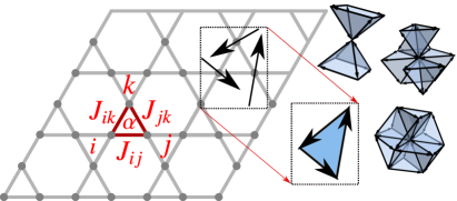
Figure 1: Illustration of finite-size kagome lattices with primitive lattice vectors $\mathbf{a}_{1}=(1,0)$ and $\mathbf{a}_{2}=(1,\sqrt{3})/2$. Classical $O(3)$ spins in triangle $\alpha$ at sites $i,j,k$ are coupled anti-ferromagnetically via $J_{ij}>0$. Groundstates are defined via local constraints $\mathbf{l}_{\alpha}=0$, such that spins on every triangular plaquette form a scalene triangle in the spin space and produce generically non-coplanar magnetic structures illustrated on the right-hand side.

Hamiltonian: We consider the classical nearest neighbour Heisenberg model

$$\mathcal{H} = \sum_{\langle ij\rangle}J_{ij}\,{\bf{s}}_{i}\cdot{\bf{s}}_{j}\ ,$$ (1)

with disordered anti-ferrromagnetic couplings $J_{ij}>0$ between $O(3)$ spins ($\left|\mathbf{s}_{i}\right|=1$) at site $i,j$ on the Kagome lattice as illustrated in Fig. 1.

The Hamiltonian can be rewritten as a sum of squares

$$\mathcal{H}=\frac{1}{2}\sum_{\alpha}{\bf{l}}_{\alpha}^{2}+\textrm{const},\quad\text{with}\quad{\bf{l}}_{\alpha}=\sum_{i\in\alpha}\gamma_{i\alpha}{\bf{s}}_{i}\,,$$ (2)

where in every triangle $\alpha$ formed by sites $ijk$ we defined $\gamma_{i\alpha}=\sqrt{{J_{ij}J_{ik}}/{J_{jk}}}$. Both forms are completely equivalent if $J_{ij}>0$ allowing to define $\gamma_{i\alpha}$.

We will mainly work with the second form, and restrict the model further by requiring $\gamma_{i\vartriangle}=\gamma_{i\triangledown}$, which corresponds to some short-range correlations of the bond-couplings. This is done mainly to reduce finite-size effects, in particular, for the ground state energy which is $E_{\rm g.s.}=0$ (ignoring the constant term) once all constraints are satisfied. The groundstates of these models exhibit different spin-spin correlations, in the first case being exponentially decaying, and in the second algebraically decaying. However, the finite temperature and dynamical behaviour appears qualitatively and quantitatively similar. This modification is not expected to change the results of this study qualitatively which has been explicitly confirmed for the dynamics.

Groundstate manifold: From Eq. 2 states that satisfy $l_{\alpha}=0$ on all triangles are seen to be ground states. This can be interpreted as the sum of spins with different length scaling factors $\gamma_{i\alpha}$ vanishing, i.e. forming a closed triangle in spin space as shown in Fig. 1. The resulting spin configuration of a single triangle is coplanar, but generally non-collinar, while on the full lattice it becomes non-coplanar as well. It may be visualised as a three-dimensional structure with scalene triangles as faces, see Fig. 1.

The fact that all constraints on the kagome lattice can be satisfied simultaneously is non-trivial. The resulting set of groundstates of the jammed spin liquid Bilitewski et al. (2017) includes exponentially many exactly degenerate non-coplanar groundstates in presence of disorder (up to a critical disorder strength), which are rigid without any zero-modes besides global rotations. In particular, they are not connected to the coplanar groundstates, which are known to determine the low-temperature properties of the non-disordered model Chalker et al. (1992); Huse and Rutenberg (1992); Reimers and Berlinsky (1993); Moessner and Chalker (1998a); Zhitomirsky (2008), and have an extensive number of zero-modes Chalker et al. (1992); Huse and Rutenberg (1992); rather they form a disconnected discrete set, instead of a continuous connected manifold Moessner and Chalker (1998a).

Dynamics: The semi-classical spin dynamics, describing precession of spins around their local exchange fields, is given by the Landau-Lifshitz equation L. D. Landau (1975),

$$\frac{d\mathbf{s}_{i}(t)}{dt}=-\mathbf{s}_{i}(t)\times\left(\sum_{j}J_{ij}\mathbf{s}_{j}(t)\right)$$ (3)

which conserves the total energy $E$, magnetisation $\mathbf{M}$ as well as the spin norm.

Global Symmetries and equivalence classes of states: The Hamiltonians in Eq. 1 and 2 possess a global $O(3)$ symmetry. The invariance of the energy under these rotations results in 3 global-zero modes of the groundstates and the conservation of the total magnetisation under the dynamics. In defining distinct states it is necessary to take these symmetries into account. Formally, one may use equivalence classes defining distinct states as spin-configurations modulus the $O(3)$ symmetry. One may transform any spin configuration to a representative of the equivalence class, e.g. by rotating the spins such that ${s}_{1}$ points in a fixed direction by using a global rotation of all spins and $\mathbf{s}_{2}$ lies in a fixed plane by rotating all spins around $\mathbf{s}_{1}$, and compare spin configurations after rotating into this fixed frame. Alternatively, the gram-matrix $g_{ij}=\mathbf{s}_{i}\cdot\mathbf{s}_{j}$ uniquely characterises distinct equivalence classes accounting for the rotational symmetry automatically. In practice, we choose to work with explicit representatives by rotating into a fixed frame for this study.

Details on the numerics: We perform both Monte-Carlo simulations to obtain finite temperature spin configurations and explicit energy minimisation to obtain ground state spin configurations. Both are combined with molecular dynamics simulations Moessner and Chalker (1998a, b); Conlon and Chalker (2009); Robert et al. (2008); Taillefumier et al. (2014).

For the ground state simulations states are converged to an energy of $E<10^{-14}$, or until the norm of the energy-gradient is smaller than $10^{-8}$ (in case we end up in a local minimum).

The Monte-Carlo simulations are performed using heat-bath updates combined with micro-canonical overrelaxation updates. From these we obtain samples from the Boltzmann distribution $\sim\exp[-\beta\mathcal{H}]$ at inverse temperature $\beta$.

Taking the samples obtained via Monte-Carlo as initial conditions, the equations of motion Eqs. 3 are integrated numerically, and quantities of interest computed from the time-evolved spin configuration. Thus, the ensemble averaged is approximated by an average over different initial states $\left<\mathbf{s}_{i}(t)\cdot\mathbf{s}_{j}(0)\right>\approx 1/N_{\textrm{states}}\sum_{\textrm{states}}\mathbf{s}_{i}(t)\cdot\mathbf{s}_{j}(0)$. Time integration is performed using a fourth-order Runge-Kutta algorithm with adaptive time step size such that the error on the conserved energy, spin-length and magnetisation remains below $10^{-6}$ per spin.

We study systems up to linear system size $L=24$ (corresponding to $N_{s}=1728$ spins) with explicit energy-minimisation, and systems up to $L=96$ ($N_{s}=27648$) and temperatures $\beta=1,\cdots,10000$ with MC.

Throughout we work in dimensionless units with the lattice spacing $a=1$. We choose the couplings $\gamma_{i}=1+\delta_{i}$ with $\delta_{i}$ uniformly in $[1-\delta,1+\delta]$ for disorder strength $\delta$. We also restrict to $\delta=0.3$ in this work, but have checked that results are qualitatively the same within the jammed spin liquid regime $\delta<1/3$. Results are averaged over 100 disorder realisations for the groundstate simulations, and over a 1000 disorder realisations for the MC simulations.

III Spin stiffness

III.1 Analytical derivation

The spin stiffness is defined via the energy response to a twist, i.e. via comparing the energy of states obtained with periodic boundary conditions (PBC), and those with twisted boundary conditions along one of the lattice directions. Specifically, we take $\mathbf{S}_{i+Le_{x}}=R(\theta,\mathbf{e}_{\theta})\mathbf{S}_{i}$ with a rotation matrix $R$ depending on the twist angle $\theta$ and the rotation axis $\mathbf{e}_{\theta}$. The energy difference between PBC and twisted BC follows as the minimum over all possible orientations of the rotation axis $\mathbf{e}_{\theta}$.

The vanishing spin stiffness in the jammed spin liquid regime can be derived from considerations of the constraints defining the set of ground states, together with the implicit function theorem. Specifically, we have that for groundstates $\mathbf{l}_{\alpha}=0$ on all triangles $\alpha$. Imposing twisted boundary conditions amounts to changing the energy function in the border triangles in the following way:

$$(\gamma_{a}\mathbf{S}_{a}+\gamma_{b}\mathbf{S}_{b}+\gamma_{c}\mathbf{S}_{c})^{2}\rightarrow(\gamma_{a}\mathbf{S}_{a}+\gamma_{b}\mathbf{S}_{b}+R(\theta,e_{\theta})\gamma_{c}\mathbf{S}_{c})^{2}$$ (4)

Thus, the zero-energy groundstates can still be written as a sum of squares, and we have a mapping

$$\begin{split}G:\quad&\mathbb{R}\times\mathbb{R}^{3N_{\mathrm{s}}}\rightarrow\mathbb{R}^{3N_{\mathrm{s}}}\\ &\theta\times\{\mathbf{S}_{i}\}\mapsto\begin{cases}\mathbf{S}^{2}_{i}-1&i\in 1,\dots,N_{S}\\ {\bf{l}}_{\alpha}(\theta)&\alpha\in 1,\dots,2N_{\mathrm{s}}/3\end{cases}\end{split}$$ (5)

where now ${\bf{l}}_{\alpha}$ depends on the twisting angle $\theta$. The ground state configurations for PBC then correspond to the preimage of the zero-vector, e.g. $\{\mathbf{S}^{\mathrm{gs}}_{i}\}=G^{-1}(\mathbf{0})$.

Given a ground state for PBC, e.g. a point $\{\theta_{0}=0,\{\mathbf{S}_{i}\}\}$ such that $G(\{\theta_{0},\{\mathbf{S}_{i}\}\})=\mathbf{0}$, the implicit function theorem guarantees that the ground state is given by a differentiable function of the twist angle $\theta$ in an open neighbourhood of $\theta_{o}$ if the Jacobian $\left[\frac{\partial G_{i}}{\partial S_{jd}}\right]$ is invertible. Here $j=1,\dots,N_{\mathrm{s}}$ is the site index and $d=x,y,z$ is the index of the spatial dimension.

Since $R(0,e_{\theta})=1$ and our previous work already established the non-vanishing of the Jacobian determinant for JSL ground states Bilitewski et al. (2017), we conclude that we can continue these states over a finite range of twisting angles $\theta$ with exactly vanishing energy, thus establishing the vanishing of the spin stiffness in the jammed spin liquid.

III.2 Numerical Results

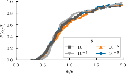
Figure 2: Cumulative distribution $F(x)=\int_{0}^{x}p(y)dy$ of the scaled mean angle $\bar{\alpha}/\theta$ between states found for periodic boundary conditions and the one after applying a twist for twist angles $\theta=10^{-3}$ down to $\theta=10^{-6}$ obtained from 100 different ground states and disorder configurations.

Beyond this proof of vanishing spin stiffness we consider the response of the system to a twist in more detail numerically. To do so we obtain a ground state for PBC via energy minimisation starting from a random initial configuration, then apply the twist and start the energy minimisation from the previously found state.

As a first check on the numerics, and to ensure that the $\theta$-range over which states can be continued is (sufficiently) large in practice, we compute the average rotation angle between the spin configuration found for twisted BC and the one for PBC defined as

$$\bar{\alpha}=1/N_{s}\sum_{i}\arccos(\mathbf{S}^{PBC}_{i}\cdot\mathbf{S}^{TBC}_{i}(\theta))\,.$$ (6)

This should stay small and be linear in $\theta$, such that the twisted state remains close to the initial state, and the energy difference actually is a measure of the spin stiffness of that state.

We show the cumulative distribution function of the scaled twist angle $\bar{\alpha}/\theta$ obtained from 100 different disorder realisations and states on a $L=12$ system in Fig. 2 for a range of twisting angles $\theta=10^{-6}$ up to $10^{-3}$. The collapse of the data confirms the expected linear scaling of the response to the twist which remains on the natural order of $\theta$.

Importantly, we find the energy difference to vanish within the numerical accuracy for sufficiently small twist angles, specifically we checked it for twisting angles $\theta=10^{-6}$ up to $\theta=10^{-3}$ for different initial states and disorder realisations and different system sizes $L=6,12$, i.e. we confirm the vanishing of the spin stiffness also numerically.

IV Spin Dynamics

IV.1 Spin Autocorrelation

The simplest indicator of the nature of spin dynamics is the spin autocorrelation function defined as

$$A(t)=\frac{1}{N}\sum_{i}\left<\mathbf{s}_{i}(t)\cdot\mathbf{s}_{i}(0)\right>\,,$$ (7)

which may be interpreted as the overlap between the initial and time-evolved state.

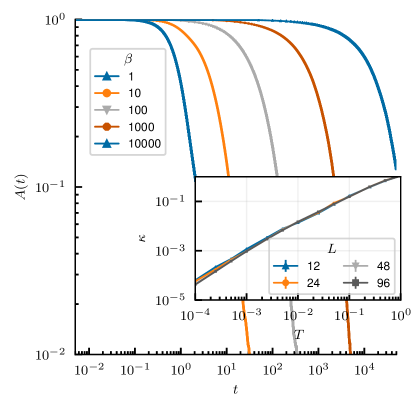
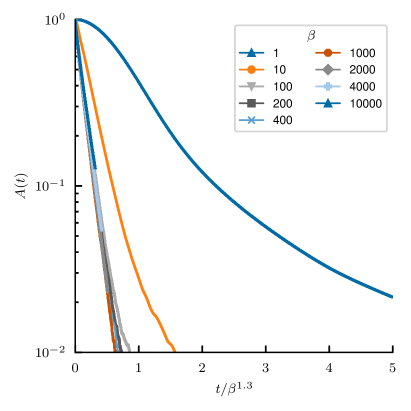
Figure 3: Main: Spin autocorrelation on a $L=96$ system at temperatures $\beta=1,\cdots,10000$ as indicated in the legend Top on log-log scale versus time $t$, bottom on log-linear scale versus scaled time $t/\beta^{1.3}$. Inset: Extracted exponential decay constant $A(t)\sim e^{-\kappa t}$ versus temperature $T$ for different system sizes $L=12,24,48,96$ as in the legend.

In Fig. 3 we show the spin autocorrelation on a $L=96$ system for a range of temperatures $\beta=1,\cdots,10000$ as a function of time $t$.

In the short time-regime at large temperatures we observe an initial quadratic regime, followed at very long times by a diffusive tail $A(t)\sim 1/t$ due to the conservation of the total magnetisation. This is expected at large temperatures and times Müller (1988); *Gerling1989; *Mueller1989; Gerling and Landau (1990), and has been established for the clean Kagome AFM Robert et al. (2008); Taillefumier et al. (2014).

For lower temperatures the quadratic regime shrinks (and we do not access sufficiently large times to see the diffusive tail), and the behaviour crosses over into a purely relaxational exponential decay $A(t)\sim e^{-\kappa t}$.

We extract the decay rate $\kappa$ from the auto-correlation by fitting an exponential in the time window $0<t<5\beta$ and for $A(t)>10^{-2}$. The decay rate $\kappa(T)$ is found to be temperature-dependent as seen in the inset Fig. 3 showing the decay rate extracted for different system sizes versus temperature $T$. Whereas the intermediate temperature range $10<\beta<100$ is consistent with a linear scaling $\kappa(T)\sim T$, at the lowest temperatures $10^{2}<\beta<10^{4}$ the exponent seems to increase to about $\kappa(T)\sim T^{1.3}$ The upper intermediate linear scaling is consistent with the behaviour found for the classical spin liquid on the non-disordered Kagome Robert et al. (2008); Taillefumier et al. (2014), and the pyrochlore lattice Conlon and Chalker (2009), as well as the predictions of the large-N calculations Conlon and Chalker (2009); Taillefumier et al. (2014), whereas the $T^{1.3}$ at lowest temperatures deviates from previously seen behaviour. However, we cannot definitely say that this defines a new regime, or if there is a further crossover as temperature approaches $0$.

IV.2 Structure Factor

Spin correlations are captured by the dynamical structure factor

$$\mathcal{S}(\mathbf{q},t)=\left<\mathbf{s}(\mathbf{q},t)\cdot\mathbf{s}(-\mathbf{q},0)\right>$$ (8)

where $\mathbf{s}(\mathbf{q},t)=\sum_{i}\mathbf{s}_{i}(t)e^{-i\mathbf{R}_{i}\cdot\mathbf{q}}$ is the spatial Fourier transform of the spin configuration. Its frequency transformed version $\mathcal{S}(\mathbf{q},\omega)$ maps the spectrum of the dynamical spin-pair correlations, while the quasi-elastic limit $\mathcal{S}(\mathbf{q},\omega=0)$ is sensitive to the presence of order in the system.

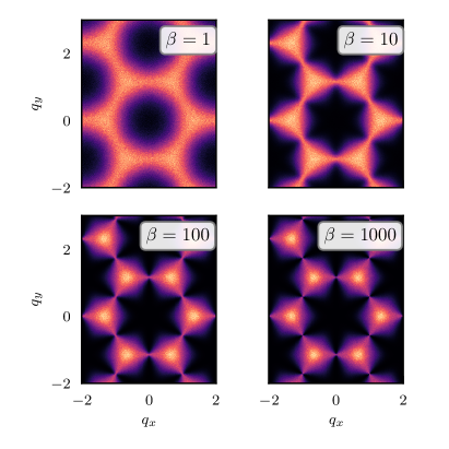
Figure 4: Quasi-elastic structure factor $\mathcal{S}(\mathbf{q},\omega=0)$ as a function of momentum for $\beta=1,10,100,1000$ as indicated in the panel.

Quasi-elastic structure factor: The quasi-elastic structure factor $\mathcal{S}(\mathbf{q},\omega=0)$ in momentum space for different temperatures, $\beta=1,10,100,1000$, is shown in Fig. 4. These temperatures span the regime from paramagnetic down to the fully established cooperative spin liquid regime for $\beta\gtrsim 10$.

At the largest temperature $\beta=1$ the structure factor only has broad features in momentum space due to the strong thermal fluctuations in the paramagnetic state. In the cooperative regime triangular structures of strong intensity emerge, and with lowering temperature intensity is transferred to the centers of these regions, which however do not correspond to Bragg peaks as there is no long-range order. The quasi-elastic structure factor does not change considerably above $\beta=100$, and does not indicate any long-range order down to $\beta=10000$, consistent with our previous findings. In particular, note the absence of the $\sqrt{3}$-satellite-peaks which would be present in the clean model Zhitomirsky (2008).

Dynamical structure factor:

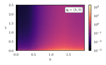
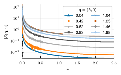
Figure 5: Top: Intensity map of the dynamical structure factor $|\mathcal{S}(\mathbf{q},\omega|)$ versus momentum $\mathbf{q}=(h,0)$ and frequency $\omega$ at a temperature $\beta=100$. Colormap on a logarithmic scale. Bottom: Selected cuts of the same data, $\mathcal{S}(\mathbf{q},\omega)$ as a function of $\omega$ for fixed momenta $\mathbf{q}=(h,0)$ as indicated in the legend.

The dynamical structure factor $\mathcal{S}(\mathbf{q},\omega)$ only shows broad features in momentum and frequency space as shown in Fig. 5 at a temperature of $\beta=100$ along a momentum cut from the BZ centre to the edge, $\mathbf{q}=(h,0)$.

This suggests that there are no sharp spinwaves present in the disordered model, even at temperatures where they are seen in the clean system Robert et al. (2008).

In addition, some spectral weight is highly concentrated at small frequencies as seen in the bottom panel of Fig. 5. We associate this with the large number of soft normal modes discussed below in terms of the Hessian matrix of ground states.

Diffusion:

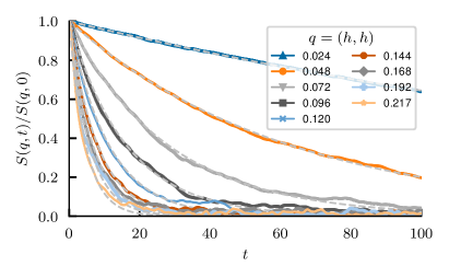
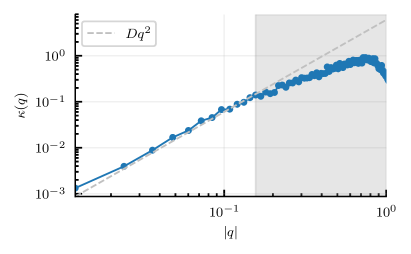
Figure 6: Top: Cuts of dynamical structure factor $\mathcal{S}(\mathbf{q},t)$ for momenta $\mathbf{q}=(h,h)$ close to the Brillouin zone center versus time $t$ for temperature $T=0.1$, dashed gray lines are fits to an exponential decay $\mathcal{S}(\mathbf{q},t)\sim e^{-\kappa(q)t}$ Bottom: Extracted decay constant $\kappa(q)$ versus momentum $|q|$ with a quadratic fit $\kappa(q)=Dq^{2}$ (dashed line), shaded area denotes where quadratic fit ceases to be valid.

Cuts of the dynamical structure factor $\mathcal{S}(\mathbf{q},t)$ as a function of time $t$ at fixed momentum $q=(h,h)$ close to the Brillouin zone center are shown in Fig. 6. We observe an exponential decay in time $S(\mathbf{q},t)\sim e^{-\kappa(\mathbf{q})t}$ with a momentum dependent decay rate.

The decay rate itself depends quadratically on momentum $\kappa(\mathbf{q})=Dq^{2}$ (lower panel of Fig. 6), at least for sufficiently small momenta close to the center of the BZ. This in turn allows us to obtain the diffusion constant $D$.

We note that the range of validity of this quadratic dependence shrinks with temperature, a behaviour already observed in the clean Kagome magnet Taillefumier et al. (2014). In addition, the functional form above this threshold momentum changes, flattening into a plateau of constant decay-rate. However, we cannot exclude that diffusion still takes place at smaller wave-vectors, or larger length scales than we can access in the simulations.

We also note that since the decay rate of the auto-correlation function, which corresponds to some average of the decay-rates of the momentum-resolved structure factor, continues to decrease with temperature, the range of the quadratic behaviour must decrease and/or the the diffusion constant must decrease at low temperatures.

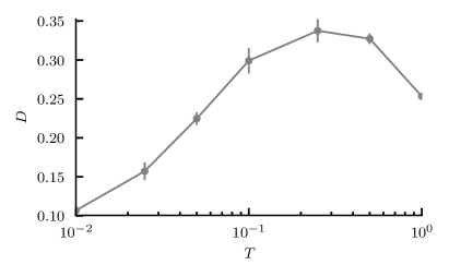
Figure 7: Diffusion constant $D$ as a function of temperature $T$ as extracted from the quadratic dependence of the decay-rate of the dynamical structure factor.

The extracted diffusion constant $D$ as a function of temperature $T$ is shown in Fig. 7. Upon lowering the temperature, we first observe an increase, comparable to the one observed in the clean model on the transition from high-temperature paramagnetic states to the cooperative paramagnetic regime.

On further lowering the temperature, the diffusion constant starts to decrease. This is in stark contrast to the situation of the clean model for which the diffusion constant after reaching a “plateau” in the cooperative regime seems to diverge on approaching the octupolar regime Taillefumier et al. (2014). In any case, the observed decrease it relatively slow, and the data does not allow to conclude if it will continue down to lower temperatures or if it saturates to a finite value.

IV.3 Finite-size Transition to Dynamically Arrested States

On finite systems we observe a transition into a dynamically arrested state. In the arrested regime the dynamics is stuck close to a single groundstate and does not explore the full phase space. Dynamics in this regime can be understood as fast small oscillations around a fixed state in combination with a slow global precession of all spins.

We characterise the dynamical arrest by considering a modified spin autocorrelation function $A_{mod}(t)$ obtained by globally rotating all spins of the time-evolved state such that the first spin $\mathbf{s}_{1}(t)$ points in the same direction as $\mathbf{s}_{1}(t=0)$ and the second spin $\mathbf{s}_{2}(t)$ lies in the same plane as $\mathbf{s}_{2}(t=0)$. Intuitively, in this way we remove the zero-energy modes due to the global $SO(3)$ invariance of the Hamiltonian, and the rather trivial dynamics of a rigid rotation of all spins which should not be considered to lead to a different state. Since we globally rotate all spins, and then rotate all other spins around a single spin $S_{1}$, this leaves the energy invariant.

This was not required for the dynamics discussed above, but becomes so now for the parameters considered here. At the low temperatures/energy densities at which we observe the freezing transition the dynamics has slowed down so much that a global slow precession of the state masks the internal dynamics of the spin state, whereas at larger temperatures the internal dynamics are fast enough to be fully resolved before the global precession becomes relevant.

We either sample states via MC from the Boltzmann distribution at a finite (small) temperature, or add a (small) energy density to a GS obtained from numerical minimisation of the energy by rotating all spins slightly in their local exchange fields.

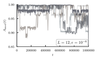
Figure 8: Selected individual time-traces of the modified spin-autocorrelation function $A_{\textrm{mod}}(t)$ for a fixed disorder realisation on a $L=12$ system and an added energy density $e=10^{-6}$ above different groundstates.

For illustrational purposes we begin by discussing individual time-traces at a fixed disorder realisation of the modified autocorrelation function at low energy densities above a ground state close to the dynamic arrest in Fig. 8. Note in particular the extremely large times up to $t=10^{6}$ over which we resolve the dynamics here. We emphasise that these are fixed disorder trajectories at smaller energy densities and on a different time-scale than the disorder-averaged spin-spin autocorrelation results in Fig. 3, which still would have fully decayed by these times if the previously observed scaling did persist down to these energies.

In stark contrast to the previously discussed (exponentially) decaying autocorrelation, here we observe rapid oscillations around a fixed plateaus for long time periods separated by rapid and sudden transitions to different plateaus. We interpret this behaviour as the system system being stuck close to distinct ground states as characterised by the distinct plateaus for long times, around which it performs small normal mode oscillations, until a sudden and sharp transition to different plateau/state occurs.

Furthermore, in this regime the system remains close to the original state, in that we observe transitions out of and back into the original state, and in some cases repeatedly to the same distinct plateau/state. This would be exceedingly unlikely if the dynamics were to explore the full exponentially large groundstate manifold of the jammed spin liquid.

This behaviour is somewhat reminiscent of (finite) spin glass systems which are stuck for (exponentially) long times in some part of phase space, but may suddenly jump to a distinct region Parisi (2006). These distinct states might also lend themselves to the interpretation of two-level systems, as observed in Heisenberg spin glasses Baity-Jesi et al. (2015), and do indicate some form of clustering of the ground states.

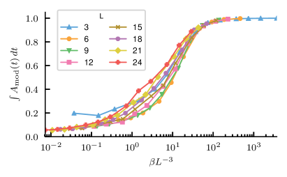
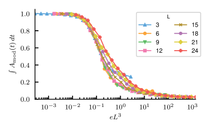
Figure 9: Top: Long time average of the (modified) spin autocorrelation function $A_{mod}$ versus scaled temperature $\beta L^{-3}$ in the MC simulations. Bottom:Long time average of the (modified) spin autocorrelation function of groundstates with an added energy density $e$ created by randomly rotating spins in their local exchange fields.

The long-time average of the modified autocorrelation function averaged over disorder realisations is shown in Fig. 9, averaged over initial states obtained from MC-simulations at a finite temperature (top panel), and as a function of energy density added to a true groundstate ($E=0$) by randomly rotating the spins in their local exchange field (bottom panel). (We have checked that the same transition with the same scaling occurs for the random bond model.)

The finite temperature Monte Carlo results display a clear crossover as a function of temperature between dynamics which explores (some of) phase space and $A_{mod}\approx 0$, and dynamics at low temperatures which is stuck near a single groundstate with $A_{mod}\approx 1$. Similarly, the groundstate simulations show a transition as a function of added energy density with the same scaling.

We note that the transition to a dynamically arrested state appears to be a finite size effect, in that the temperature below which the dynamics is arrested scales as $T\sim L^{-3}$ for the MC simulations, and energy density $e\sim L^{-3}$ for the groundstate simulations. This leads us to conclude that the energy barriers between different JSL groundstates vanish in the thermodynamic limit.

V Hessian

To elucidate the behaviour found above, we first investigate the statistical properties of an individual local extremum, before turning to their connectivity properties in the following sections.

Following on from our original work Bilitewski et al. (2017), we investigate the quadratic energy cost of fluctuations around groundstate configurations via the Hessian matrix. This provides insight into the spectrum of fluctuations, potential low-energy or zero-modes, and via the associated eigenvectors also into the spatial properties of these normal modes.

For a spin configuration $\left\{\mathbf{s}_{i}\right\}$ we choose an orthonormal local basis at every lattice site $(\mathbf{s}_{i},\mathbf{u}_{i},\mathbf{v}_{i})$. This allows us to parametrise fluctuations as $\mathbf{\tilde{s}}_{i}=\sqrt{1-\epsilon_{i}^{2}}\mathbf{s}_{i}+\epsilon_{ui}\mathbf{u}_{i}+\epsilon_{vi}\mathbf{v}_{i}$ with $\epsilon_{i}=(\epsilon_{ui},\epsilon_{vi})$ which takes the spin normalisation condition into account. Around a groundstate the energy-cost of fluctuations to quadratic order is then given by $E=\epsilon^{T}M\epsilon$, which defines the $(2N_{s})\times(2N_{s})$ Hessian matrix $M$.

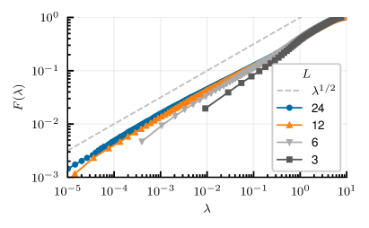
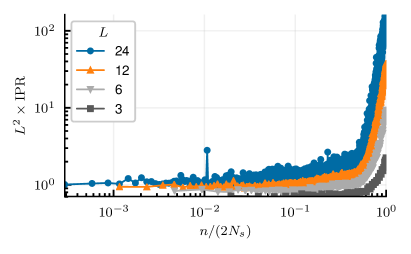
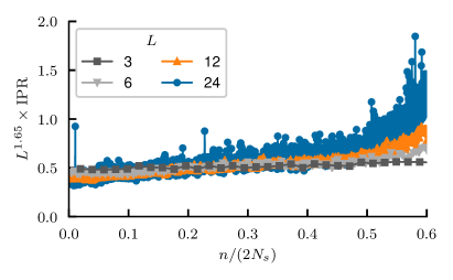
Figure 10: Top: Cumulative distribution function $F(\lambda)$ of the eigenvalues $\lambda$ of the Hessian matrix of groundstates for different linear system sizes $L$ as indicated in the legend, and $\lambda^{1/2}$ powerlaw behaviour (dashed) line Middle and Bottom: Inverse participation ratio (IPR) of eigenstate $n$ of the Hessian ordered by eigenvalue, middle scaled with $L^{2}$ on log-log scale, bottom scaled with $L^{1.65}$ on linear scale focussing on the soft modes.

Diagonalising the Hessian matrix $M$ provides eigenvalues $\lambda$ and the corresponding eigenmodes. Due to the global rotational invariance of the energy there are 3 trivial zero-modes which we do not consider below.

We analyse the spectrum by considering the cumulative distribution function $F(\lambda)=\int_{0}^{\lambda}P(x)\,\textrm{d}x$ of the Hessian eigenvalues averaged over disorder which is shown in Fig. 10. Note that this has the advantage of being mostly independent of system size, with larger systems simply extending the results down to smaller eigenvalues. We observe a large number of soft-modes with a low energy scaling $F(\lambda)\sim\lambda^{1/2}$. In that sense the jammed spin liquid states are marginally stable, as soft modes extend as a powerlaw to zero energy. Crucially, there are no non-trivial zero-modes, in contrast to the coplanar states of the clean Kagome system which hosts an extensive number of these.

Secondly, we study the localisation properties of these modes by considering the inverse participation ratio (IPR) Mazzacurati et al. (1996); Bell and Dean (1970) defined as

$$\textrm{IPR}=\sum_{i}{\left(\left|\epsilon_{i}\right|^{2}\right)^{2}}/\sum{\left|\epsilon_{i}\right|^{2}}\,,$$ (9)

which is 1 for an eigenmode fully localised on a single site of the lattice, and $1/N_{s}\sim L^{-2}$ if it is fully delocalised.

The IPR is shown in the bottom panels of Fig. 10 for different linear system sizes $L$. We observe a tendency towards delocalisation for most of the spectrum, in particular for the soft modes, with a best fit fractal exponent $\textrm{IPR}\sim L^{-5/3}$. In contrast, the “hardest” modes at the upper edge of the spectrum are strongly localised to a few sites.

This is notable since the coplanar states of the clean model have an extensive number of localised zero-energy modes, in particular the $\sqrt{3}\times\sqrt{3}$ state admits hexagon weatherwane modes involving only 6 sites, and the $q=0$ state admits modes which involve $L$ sites.

These results confirm the picture that the ground states of the jammed spin liquid have no non-trivial zero-modes, but a large number of relatively soft modes. Interestingly, these soft-modes appear to be delocalised over the full lattice, rather than being local excitations like in the clean model.

VI Forcing / Spectroscopy of Energy Barriers

The results on the dynamics indicated that at sufficient energy/temperatures the system can explore a large part of phase space, whereas at low energies finite energy barriers between distinct ground states, which scale to zero in the infinite system size limit, inhibit dynamics freezing the system close to one ground state. Furthermore, the study of the Hessian showed that each local minimum has no non-trivial zero-modes, thus, locally appearing as a quadratic well in configuration space. We now set out to explicitly probe the energy barriers between distinct close groundstate configurations.

VI.1 Method

To explore the groundstate manifold further and gain insight into the energy-barriers between distinct groundstates we use the following protocol, which we adapt from its application in the study of spin glasses Baity-Jesi et al. (2015).

• Find a groundstate $\mathrm{GS}$ of original hamiltonian $\mathcal{H}$ (Eq. 2)

• Find a groundstate/local minimum $\mathrm{GS}(h)$ of a perturbed hamiltonian $\mathcal{H}_{h}$ (defined in Eq. 10) with a force/magnetic field $h$ added starting from $\mathrm{GS}(0)$

• Find a groundstate $\mathrm{GS}^{*}$ of original hamiltonian $\mathcal{H}$ starting from $\mathrm{GS}(h)$

• Compare the newly obtained groundstate $\mathrm{GS}^{*}$ with the original state $\mathrm{GS}$

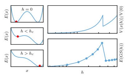
Figure 11: Illustration of the proposed forcing protocol (see text). Left panels: one-dimensional double well potential $V(x)$ with an added linear force $E(x)=V(x)+hF(x)$ proportional to $h$. Red circle denotes the state $x(h)$ at the minimal energy of the perturbed potential. Right panels: energy versus forcing strength; top for the one-dimensional toy model, bottom energy $E$ computed from $\mathcal{H}$ of the perturbed state $\mathrm{GS}(h)$ for a single realisation of the proposed forcing protocol in the full spin system.

Intuitively, this protocol can be motivated using a one-dimensional analogy as illustrated in Fig. 11. Imagine a particle in a double well potential (corresponding to two distinct ground states of the jammed spin liquid which act as quadratically confining wells). Starting with the particle in one well, one can add a linear force to make it move up the barrier towards the other well (corresponding to state $\mathrm{GS}(h)$). As long as the particle does not cross the maximal height of the barrier between the wells after removing the linear force it will fall back to the initial state (e.g. $\mathrm{GS}^{*}=\mathrm{GS})$ as seen in the middle left panel of Fig. 11. At sufficently large applied force the particle reaches the maximum of the potential between the two minima, at larger applied force it will then fall into the next well (e.g. $\textrm{GS}*\neq\textrm{GS}$ ) as seen in the lowest left panel of Fig. 11. The minimal value of the force required for this to happen then defines $h_{c}$ and the height of the barrier corresponds to the energy of the particle at $h_{c}$.

The right panels of Fig. 11 compare the resulting energy observed at a certain strength of the forcing for the toy model (top) to one realisation of the forcing protocol for the full spin-model (bottom) demonstrating qualitative agreement with this analogous model.

We define the Hamiltonian $\mathcal{H}(h)$ as

$$\mathcal{H}(h)=\mathcal{H}+h\sum_{i}\mathbf{s}_{i}\cdot\mathbf{h}_{i}$$ (10)

where we choose the magnetic fields $\mathbf{h}_{i}$ to be orthogonal to the initial groundstate $\mathrm{GS}$, i.e. $\mathbf{h}_{i}\cdot\mathbf{s}^{\mathrm{GS}}_{i}=0$, and normalised as $\sum_{i}\mathbf{h}_{i}^{2}=1$. (This is to say that the $\{\mathbf{h}_{i}\}$ form a normalised element in the tangent space of $\mathcal{S}_{2}^{N_{s}}$)

By choosing the field local and in the tangent space we avoid the issue that due to rotational invariance of the hamiltonian the main response of any state to a global field will just be to align with the field direction.

We consider different scenarios for this forcing: (a) we choose the direction of the forcing to correspond to the softest direction of the Hessian matrix of the initial groundstate $\mathrm{GS}$, (b) the hardest direction of the Hessian, and (c) a random direction in the tangent space of the initial groundstate $\mathrm{GS}$.

We emphasise that this protocol inherently goes beyond the linear response regime which would be fully captured by the eigenvalues of the Hessian. The purpose is to perturb the state strongly enough to leave the local basin of attraction of the initial state resulting in a (potentially sudden) non-linear response.

In addition, it allows us to extract (local) information about the set of groundstates which is not accessible from the states alone. Namely, we will obtain the critical fields and the height of energy-barriers between “neighbouring” (those connected by the protocol above) groundstates, and the locality of changes between these “neighbouring” states.

We note that the perturbed state $\mathrm{GS}(h)$ we obtain numerically is not necessarily a ground state of $\mathcal{H}(h)$, but rather only a local minimum. However, we are actually not interested in the ground states of $\mathcal{H}(h)$ in any case, as we only use it to perturb the original ground states in a deterministic fashion. Further starting from $\mathrm{GS}(h)$ we are not guaranteed to obtain a true groundstate $\mathrm{GS}^{*}$ of $\mathcal{H}$ with $E=0$, but may also end up in a local minimum. These cases are however easily distinguished by the non-vanishing of the energy and for the discussion below we only consider cases for which the minimisation results in a global minimum.

VI.2 Critical forcing strength

To find the critical field $h_{c}$ required to leave the basin of attraction of a given groundstate $\mathrm{GS}$, we follow the protocol outlined above. Thus, we initialise $h$ at a very small value, compute the perturbed state $\mathrm{GS}(h)$ and associated state $\mathrm{GS}*$, and increase $h$ until we encounter a new state $\mathrm{GS}^{*}\neq\mathrm{GS}$ for the first time, as characterised by an overlap with the inital state unequal to 1.

In practice starting from a ground state obtained via energy minimisation at $h=0$, we start with a small field $h\sim 10^{-7}$, increase it in powers of 10 until we find a different state, and then perform a refined search between the last two values of $h$ to determine $h_{c}$. Deciding whether a new state is encountered during this procedure poses no numerical problems as using the overlap $q$ proves sufficient given the convergence criteria put on the states (though the authors have also checked the results comparing the full gram matrix $g_{ij}=\mathbf{s}_{i}\cdot\mathbf{s}_{j}$ which is in one-to-one correspondence to spin configurations modulo global rotations).

The results for forcing in the softest and the hardest direction are shown in Fig. 12 with errors obtained from the average over 100 different disorder realisations/initial states as a function of linear system size $L$. For forcing in the softest direction we observe a vanishing of the critical field strength with system size consistent with a $L^{-3}$ scaling (dashed line).

For forcing in the hard direction the critical force first decreases, but then saturates for system sizes $L\geq 12$ at a finite value. Note also the order of magnitude difference between the critical fields.

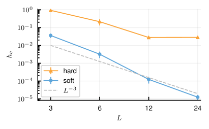
Figure 12: Comparison of critical force required to leave a groundstate for forcing in the softest direction (blue circles) and the hardest direction (orange triangles). Dashed line is a guide to the eye powerlaw $\sim L^{-3}$.

VI.3 Energy Barriers

In addition to the critical force required to leave a GS we may estimate the energy barrier between the different GS in the follwing way: As we increase $h$ we obtain a series of states $\mathrm{GS}(h)$ and associated $\mathrm{GS}^{*}$, at some critical $h_{c}$ the new state $\mathrm{GS}^{*}$ differs from the initial groundstate. We estimate the energy barrier between $\mathrm{GS}$ and $\mathrm{GS}^{*}$ by the bond-energy of the state $\mathrm{GS}(h)$, i.e. its energy with respect to $\mathcal{H}_{0}$, for $h$ just below the critical field $h_{c}$.

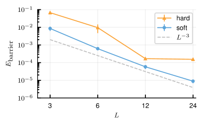
Figure 13: Comparison of energy-barriers between groundstate configurations for forcing in the softest direction (blue circles) and the hardest direction (orange triangles). Dashed line is a guide to the eye powerlaw $\sim L^{-3}$.

The results of this are shown in Fig. 13 for forcing in the softest direction and forcing in the hardest direction as a function of system size/number of spins.

We observe that for forcing in the softest direction the height of energy barriers decreases with system size as $L^{-3}$, implying that transitions between states are possible at thermodynamically vanishing energy cost.

In contrast, forcing in the hardest direction states faces a finite energy barrier which appears to saturate on larger systems consistent with the observed behaviour of the critical fields.

Whereas we cannot fully exclude any potential bias stemming from the initial ground states at larger systems which are harder to converge numerically, both the fact that the statistical errors actually decrease with increasing system size and the consistency of the ground state with Monte-Carlo simulations combined with the orders of magnitude difference between “soft” and “hard” forcing leads us to believe that this is a robust effect.

Based on the results for the critical force and the associated energy barriers, it appears that while states on finite systems have no zero-energy modes, transitions can be induced by vanishingly small forces and at vanishingly small energy cost if the force is applied in the right direction, in keeping with our results above on the stability of the arrested regime.

VI.4 Response of states to forcing

We can also characterise the response of the state to the introduced forcing by measuring its magnetisation along the applied magnetic field

$$m=\langle\mathrm{GS}(h)|h\rangle=\sum_{i}\mathbf{s}_{i}(h)\cdot\mathbf{h}_{i}$$ (11)

In Fig. 14 we again compare the forcing in the softest direction with the forcing in the hardest direction for different system sizes $L$. Note that as per the observed scaling of the critical fields above we scale the magnetic field with $L^{3}$ for forcing in the soft direction, and the resulting response by $L^{-1/3}$ to collapse data for different system sizes.

For forcing in the soft direction we observe a continuous response to the applied field. Because the energy landscape is extremely shallow in direction of the smallest eigenvector of the Hessian, the state shows a strong response to the applied field as it smoothly moves along the bottom of local basin of attraction of the initial state.

In contrast for forcing in the hard direction we observe two qualitatively distinct regimes: weak response at small fields, and above a crossover field a rapid increase of the induced magnetisation. In addition, the response is smaller in magnitude than for the soft forcing direction as expected as now the state moves along a steep direction in energy.

The observation of a “gapped” response for forcing in the hard direction is consistent with the finite critical forces and energy barriers observed above. If the field is too small to leave the initial basin of attraction, responses are weak along the steeply confined direction in configuration space, whereas when exceeding a critical field the perturbed state can escape the initial state, showing an abrupt response. After this sudden response the spin configuration ends up in a distinct state for which the forcing direction might not corespond to a strongly confined direction anymore, and for which the field direction is also not perpendicular to the state anymore, thus completely changing it’s response.

We conclude that ground states show a strongly anisotropic behaviour with order of magnitude differences in the response depending on the direction of the applied force.

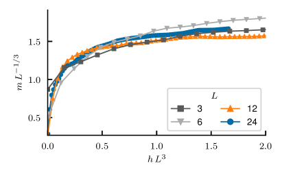
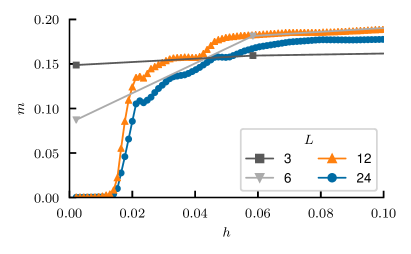
Figure 14: Comparison of the response to the applied force, i.e. the induced magnetisation, of a groundstate versus forcing strength for forcing in the softest direction (top panel) and the hardest direction (bottom panel). Note the different ranges and the differently scaled axes.

VI.5 Overlaps

We next turn to characterise the “neighbouring” states in more detail, beginning with overlaps or distances between these states, allowing us to draw conclusions on the clustering of groundstates.

We compare the original groundstate $\mathrm{GS}$ and the first different groundstate $\mathrm{GS}^{*}$ encountered when increasing the forcing strength via their average overlap $q$,

$$q=\frac{1}{N_{s}}\sum_{i}\mathbf{s}_{i}\cdot\mathbf{s}_{i}^{*}\,.$$ (12)

Again, we define this after rotating both states into a standard form with $\mathbf{s}_{1}=\mathbf{e}_{z}$, and $\mathbf{s}_{2}$ in the $xz$-plane exploiting the rotational invariance.

This provides a global notion of the total change required to transition from one GS to another, and since $|\mathbf{s}_{i}-\mathbf{s}_{i}^{*}|^{2}=2-2\,\mathbf{s}_{i}\cdot\mathbf{s}_{i}^{*}$ also geometrically corresponds to the distance between states, providing complementary information to the physical energy barriers and critical forcing fields discussed above.

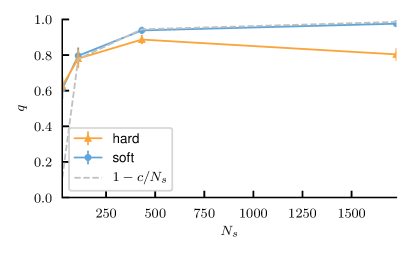
Figure 15: Comparison of overlaps for forcing in the softest direction (blue circles) and the hardest direction (orange triangles). Average overlap per spin $q=1/N_{s}\sum_{i}\mathbf{s}_{i}\cdot\mathbf{s}_{i}^{*}$.

In Fig. 15 we observe that forcing in a soft direction leads to a state $\mathrm{GS}^{*}$ with a high overlap with the original state $\mathrm{GS}$. This increases with increasing system size, converging towards $1$ as $q=1-c/N_{s}$ with a constant $c\approx 24$. This seems to suggest that, on average, only a constant number of rearrangements is required to transition into a “neighbouring” ground state, but as discussed below these rearrangements are in fact not localised, but rather require a change of all spins in the spin configuration. Thus, this result only indicates the there exist many groundstates close by.

In contrast, forcing in the hardest direction results in an overlap $q<1$, which actually tends to decrease on larger systems. However, we note that this is still relatively large considering that there are exponentially many groundstates of the JSL, and for a random new state we would expect $q\approx 0$.

This fits the interpretation that for forcing in the soft direction the GS smoothly evolves moving along a shallow basin of the energy landscape with an associated gradual change of the spins, whereas for forcing in a hard direction the evolution is along a steep direction with a sudden transition into a new basin of attraction resulting in a more strongly perturbed final spin configuration.

VI.6 Localisation of changes

Finally, we consider the locality of rearrangements required to change one groundstate into the other.

For the coplanar states of the clean model, in particular the $\sqrt{3}\times\sqrt{3}$ state, there are local zero-energy normal-modes that allow to move within the ground state manifold. For the non-coplanar groundstates of the disordered model this is not the case any longer. However, we have observed above that for forcing in a soft direction only a small change in the spin-configuration is required. Thus, it is natural to ask how this change is distributed over the lattice.

We define as the measure of localisation

$$w_{loc}=\sum_{i}{w_{i}^{2}}/\left(\sum{w_{i}}\right)^{2}$$ (13)

with $w_{i}=1-\mathbf{s}_{i}\cdot\mathbf{s}_{i}^{*}=(\mathbf{s}_{i}-\mathbf{s}_{i}^{*})^{2}/2$, analogous to the IPR discussed for the normal modes of the Hessian. It is $1$ if the change is fully local and only a single spin is changed, and $1/N_{s}$ if the change is homogeneously delocalised over all $N_{s}$ spins.

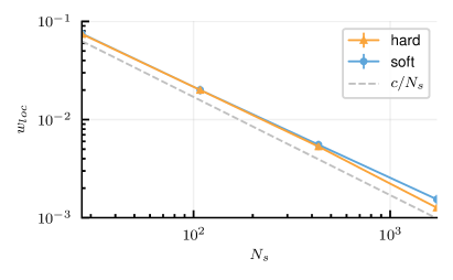
Figure 16: Comparison of localisation of changes between groundstate configurations for forcing in the softest direction (blue circles) and a random direction (orange triangles).

We show the results for forcing in the soft and the hard direction in Fig. 16. In both cases we observe a scaling $w_{loc}\sim 1/N_{s}$ corresponding to changes of the spin configuration delocalised over the full lattice.

We note that this is in agreement with the nature of the soft modes of the Hessian which we also found to be delocalised over the full lattice. However, it is in contrast to the behaviour observed in Heisenberg spin glasses, where local rearrangements between different low-lying states exist and have been found using a similiar protocol Baity-Jesi et al. (2015).

To reconcile the fact that the overlap suggests on average only a small number of changes in the spin-configuration and the delocalisation of this change over the full lattice recall that the non-disordered model has localised zero-modes and that the groundstates are defined via the set of strict constraints on each triangle of the lattice. If one now changes one spin locally, one has to change all spins in the triangles it belongs to to compensate. In turn all spins in the neighbouring triangles have to be adjusted to satisfy the constraint, continuing throughout the full lattice. It is rather remarkable that in the clean model this series of changes terminates and can be localised, whereas for the disordered spin groundstates in presence of disordered constraints it appears to require a global, but small change in the spin configuration.

VI.7 Local Forcing

Finally, we also consider a local perturbation to see whether the non-locality of the re-arrangements observed above might have been due to our globally applied field, rather than an inherent property of the probed states.

Specifically, we choose $\mathbf{h}_{i}\neq 0$ only on a single triangle $\alpha$ with a field direction $\mathbf{h}_{i}$ choosen randomly on the unit sphere. Note that applying a field local to a single spin only would, due to the rotational invariance of the field-free Hamiltonian, just lead to a global rotation of the state into field-direction, such that at least two fields are required to induce a non-trivial response. Further, a single applied field still leaves the zero mode of rotation around that field, thus even applying two local fields one encounters a zero mode. Thus, we choose a single triangle with three spins as the smallest local unit which avoids these issues.

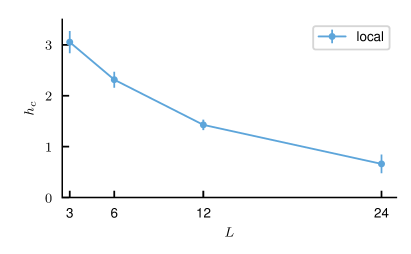
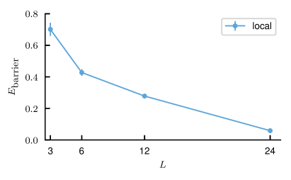
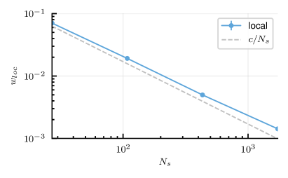
Figure 17: Top: Critical force required to leave a groundstate when applying a local field $h$ to a single triangle oriented in a random direction, middle: Corresponding energy barrier, both versus linear system size $L$ bottom: $w_{loc}$ of rearrangements between “neighbouring” groundstates, versus number of spins $N_{s}$

We again first consider the critical field strength and energy barriers in Fig. 17. We observe that even though they decrease with increasing system size, they are substantially larger than for the globally applied perturbations. Whereas we cannot make a precise statement on the asymptotic value, the fact that the Hessian of the groundstates did not have localised soft modes, and the constraints within the groundstate manifold appear locally rigid, strongly suggests that this energy cost remains finite.

The induced rearrangements of the spin-configurations after exceeding the critical field again appear to be de-localised over the full lattice (bottom panel of Fig. 17), in spite of the local nature of the applied field, lending additional confidence to the conclusion that such non-local changes are in fact required to transition to a distinct ground state.

We note that this is different from the coplanar states of the clean model, which are unstable to an infinitesimal out-of-plane local perturbation due to the local zero-modes. Indeed performing the same protocol on coplanar states of the clean model with local zero-modes the critical field as well as the energy cost vanishes, in addition to observing a finite localised response for infinitesimal applied field (as long as the out-of-plane component of the applied field is non-zero).

Thus, at least within the protocol described we do not find any local soft modes of the jammed spin liquid that would allow transitions between different ground states.

VII Random Walk in groundstate space

The discussion above provided information on the local properties of the set of groundstates, critical fields and energy barriers between “neighbouring” states. Next, we consider potential clustering and the size of the basins of attraction of different ground states, and the “connectedness” of the ground states.

To this end we propose starting from a given initial GS $\{S_{i}\}_{0}$ to repeatedly apply the procedure above to generate a sequence of states $\{S_{i}\}_{n}$, which may either be local minima or true GS, e.g.

• Find an initial ground state $\mathrm{GS}_{0}$ of $\mathcal{H}$

• in step $i$: Apply a perturbing field $h$ as detailed in sec. VI.1 starting from $\mathrm{GS}_{i-1}$, increasing the field strength until $\mathrm{GS}^{*}_{i}\neq\mathrm{GS}_{i-1}$, obtaining a new distinct state $\mathrm{GS}_{i}=\mathrm{GS}^{*}_{i}$

• repeat this $n$-times obtaining a sequence of states

In this case we mainly discuss applying the force in a random direction. Forcing the states exclusively in the softest or hardest direction as discussed above, the procedure can get stuck in a trivial cycle, typically consisting of two states connected by a steep/shallow direction in phase space respectively.

Intuitively, we expect this random walk in the space of (local) minima to be able to explore all states if the ground states form a single cluster, or get stuck in some part of the manifold if there are several disconnected clusters. We emphasise that this is slightly different to the dynamical freezing transition, as that was governed by the size of the energy barriers becoming larger than the available energy at low temperatures, whereas here we do not restrict the maximally applied field to induce a transition.

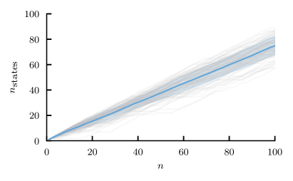
Figure 18: Number of unique encountered states $n_{\textrm{states}}$ when successively forcing the state in a random direction until a transition takes place versus number of forced transitions $n$. Light-gray lines are individual trajectories for different initial states and disorder configurations, shading is the standard deviation around the mean.

In Fig. 18 we show the number of unique encountered states $n_{\textrm{states}}$ versus the number of forced transitions $n$. Individual trajectories for different disorder configurations and initial groundstates are shown as light-gray lines, and the average with standard deviation as the blue line with shading.

From these results it appears that while individual trajectories can be stuck for some time in a set of “known” states visible in the plateaus, after a few transitions they do escape and continue to encounter successively more new states with an increasing number of transitions.

Consequently, the set of ground states appears to be connected in the sense that successive transitions through thermodynamically small energy barriers allow to explore a large number of distinct states, e.g. that if they do cluster, that these clusters are relatively large.

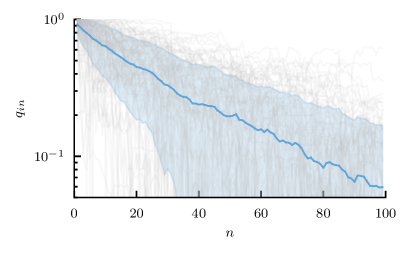
Figure 19: Overlap $q_{in}$ of the initial state with the state reached after $n$ forced transitions. Light-gray lines are individual trajectories for different initial states and disorder configurations, shading is the standard deviation around the mean.

Finally, we consider the overlap $q_{in}$ between the initial state and the state reached after $n$ transitions in Fig. 19. This is observed to decay exponentially with the number of forced transitions. Changes in states appear global, i.e. all spins are changed in every step, but the loss of overlap is incremental, i.e. we perform a succession of “small” steps in an exponentially large space, ultimately completely decorrelating from the initial state.

We emphasise that this is very different to the situation expected on the basis of replica symmetry breaking in a spin glass Marinari et al. (2000) which results in a hierachical energy landscape Parisi (1979); Mézard et al. (1984); Mezard et al. (1986); Charbonneau et al. (2014), and consequently states stuck in one local basin in which states have a high overlap, separated from distinct basins by large energy barriers Berthier and Biroli (2011); Parisi (2006); Charbonneau et al. (2014); Gonzaled-Adalid Pemartin et al. .

Thus, it appears that the set of ground states remains (at least partly) connected at finite temperatures and can via finite perturbations explore a large number of states via successive transitions reaching states fully unrelated to the initial state.

VIII Conclusions

In this work we have studied the dynamics and energy landscape of the recently identified jammed spin liquid, which has exponentially many exactly degenerate groundstates in presence of disordered bond couplings.

Since these states are rigid, e.g. they have no zero-energy modes besides global rotations, they form a discrete set, in contrast to previously studied classical spin liquids with continuous groundstate manifolds with zero-modes. Despite the rigidity of the spin ground state configurations there still exist a large number of very soft normal modes, which appear delocalised with a best-fit fractional exponent $L^{-5/3}$.

In spite of the rigidity of the ground states, we establish a vanishing spin-stiffness. The spin autocorrelation shows typical classical spin-liquid behaviour with an exponential decay rate scaling linearly with temperature in the intermediate low temperature regime and steepening to $T^{1.3}$ at the lowest temperatures we access. We also find evidence of spin diffusion, and obtain a spin diffusion constant $D$ that seems to decrease in the low temperature regime. However, we are not able to resolve whether diffusion persists down to the lowest temperatures on larger and larger length-scales with a finite diffusion constant or disappears completely.

Furthermore, the dynamical structure factor has no sharply defined features, suggesting that there are no sharp spinwaves present in the disordered model, but shows concentration of spectral weight at low frequencies, which we attribute to the large number of soft normal modes of the ground states.

Interestingly, we find a transition (on finite systems) between dynamics that is able to explore (some parts) of phase space and fully decorrelate from the original state, and a dynamically arrested regime, in which the states mostly globally rotate and perform small oscillations being stuck close to an initial state.

This in turn motivated the detailed study of the energy landscape in terms of response to forcing of the groundstates. We find that energy barriers between different groundstates vanish with increasing system size, implying that excitations, due to finite temperature or perturbations, are able to induce groundstate transitions. However, there appear to be no local rearrangements between different groundstates, transitions always requiring a global change in the spin configuration.

We find that the response is “anisotropic”, and depends on the form of the applied force: it is “gapped” for forcing in a hard direction, defined via the spectrum of the Hessian, whereas in a “soft” or random direction it smoothly evolves as a function of the forcing strength. Moreover, local forcing encounters significantly higher energy barriers and requires larger forcing fields, which we attribute to the fact that groundstate configurations are locally rigid and, thus, resist deformation.

Finally, a random walk via successive transitions is able to fully decorrelate the resulting spin configuration from the initial state in an exponential fashion, suggesting that the set of ground states remains (at least partly) connected, and that clusters, if they exist, contain a large number of quite distinct ground states.

Summarising, we find a complex energy landscape with exponentially many degenerate discrete locally rigid ground states in a bond-disordered frustrated magnet, which at finite temperatures or energy densities appear to be connected within Landau-Lifshitz spin dynamics, with exponentially decaying spin auto correlations and no sharply defined features in the dynamical structure factor, and via applied fields, with vanishing energy barriers between “neighbouring” distinct groundstates.

We finish by pointing out avenues for further research and open questions. Firstly, in the kagome Heisenberg antiferromagnet bond disorder does completely eliminate all zero-modes of the ground states. In light of the recent connections of frustrated magnetism to topology via spin-origami in the case of anisotropic interactions in the kagome HAFM Roychowdhury and Lawler (2018); Roychowdhury et al. (2018), where extensive or sub-extensive numbers of zero-modes were found protected by topological indices, a study of the (potential) topological features of the jammed spin liquid, which lifts these degeneracies completely, might provide further insight into the interplay of frustration and topology in magnets.

Secondly, the arrested regime, with dynamics observed to be “stuck” close to a state interrupted by sudden transitions between distinct states, is reminiscent of the behaviour in Heisenberg spin glasses Baity-Jesi et al. (2015); Parisi (2006). Whereas this regime vanishes in the thermodynamic limit in this model, the presence of this “glassy” phase in a model with exactly degenerate states on finite systems might provide further insight into mechanisms of spin-freezing and spin glasses.

Acknowledgments: This work was in part supported by Deutsche Forschungsgemeinschaft via SFB 1143.

References

- Reidys and Stadler (2002) C. M. Reidys and P. F. Stadler, “Combinatorial landscapes,” SIAM Review 44, 3–54 (2002).
- Franz et al. (2017) S. Franz, G. Parisi, M. Sevelev, P. Urbani, and F. Zamponi, “Universality of the sat-unsat (jamming) threshold in non-convex continuous constraint satisfaction problems,” SciPost Phys. 2, 019 (2017).
- Edwards and Anderson (1975) S. F. Edwards and P. W. Anderson, “Theory of spin glasses,” Journal of Physics F Metal Physics 5, 965–974 (1975).
- Mézard et al. (1984) M. Mézard, G. Parisi, N. Sourlas, G. Toulouse, and M. Virasoro, “Nature of the spin-glass phase,” Phys. Rev. Lett. 52, 1156–1159 (1984).
- Mezard et al. (1986) M. Mezard, G. Parisi, and M. Virasoro, Spin Glass Theory and Beyond (WORLD SCIENTIFIC, 1986).
- Young (1997) A. P. Young, Spin Glasses and Random Fields (WORLD SCIENTIFIC, 1997).
- Charbonneau et al. (2014) P. Charbonneau, J. Kurchan, G. Parisi, P. Urbani, and F. Zamponi, “Fractal free energy landscapes in structural glasses,” Nature Communications 5, 3725 (2014).
- Charbonneau et al. (2017) P. Charbonneau, J. Kurchan, G. Parisi, P. Urbani, and F. Zamponi, “Glass and jamming transitions: From exact results to finite-dimensional descriptions,” Annual Review of Condensed Matter Physics 8, 265–288 (2017).
- (9) I. Gonzaled-Adalid Pemartin, V. Martin-Mayor, G. Parisi, and J. J. Ruiz-Lorenzo, “Numerical study of barriers and valleys in the free-energy landscape of spin glasses,” arXiv:1811.03414 .
- Liu and Nagel (2010) A. J. Liu and S. R. Nagel, “The jamming transition and the marginally jammed solid,” Annual Review of Condensed Matter Physics 1, 347–369 (2010).
- Liu and Nagel (1998) A. J. Liu and S. R. Nagel, “Nonlinear dynamics: Jamming is not just cool any more,” Nature 396, 21–22 (1998).
- O’Hern et al. (2003) C. S. O’Hern, L. E. Silbert, A. J. Liu, and S. R. Nagel, “Jamming at zero temperature and zero applied stress: The epitome of disorder,” Phys. Rev. E 68, 011306 (2003).
- Berthier and Biroli (2011) L. Berthier and G. Biroli, “Theoretical perspective on the glass transition and amorphous materials,” Reviews of Modern Physics 83, 587–645 (2011).
- Behringer and Chakraborty (2019) R. P. Behringer and B. Chakraborty, “The physics of jamming for granular materials: a review,” Reports on Progress in Physics 82, 012601 (2019).
- Onuchic et al. (2000) J. N. Onuchic, H. Nymeyer, A. E. García, J. Chahine, and N. D. Socci, “The energy landscape theory of protein folding: Insights into folding mechanisms and scenarios,” in Advances in Protein Chemistry (Elsevier, 2000) pp. 87–152.
- Heidrich et al. (1991) D. Heidrich, W. Kliesch, and W. Quapp, Properties of Chemically Interesting Potential Energy Surfaces (Springer Berlin Heidelberg, 1991).
- Wright (1932) S. Wright, “The roles of mutation, inbreeding, crossbreeding and selection in evolution,” Proceedings of the Sixth International Congress of Genetics 1, 356–366 (1932).
- Mustonen and Lässig (2009) V. Mustonen and M. Lässig, “From fitness landscapes to seascapes: non-equilibrium dynamics of selection and adaptation,” Trends in Genetics 25, 111–119 (2009).
- Stadler (2002) P. F. Stadler, “Fitness landscapes,” in Biological Evolution and Statistical Physics, edited by M. Lässig and A. Valleriani (Springer Berlin Heidelberg, Berlin, Heidelberg, 2002) pp. 183–204.
- Hartl (2014) D. L. Hartl, “What can we learn from fitness landscapes?” Current Opinion in Microbiology 21, 51–57 (2014).
- Barahona (1982) F. Barahona, “On the computational complexity of ising spin glass models,” Journal of Physics A: Mathematical and General 15, 3241 (1982).
- Anderson (1956) P. W. Anderson, “Ordering and antiferromagnetism in ferrites,” Phys. Rev. 102, 1008–1013 (1956).
- Villain (1979) J. Villain, “Insulating spin glasses,” Zeitschrift für Physik B Condensed Matter 33, 31–42 (1979).
- Chalker et al. (1992) J. T. Chalker, P. C. W. Holdsworth, and E. F. Shender, “Hidden order in a frustrated system: Properties of the heisenberg kagomé antiferromagnet,” Phys. Rev. Lett. 68, 855–858 (1992).
- Moessner and Chalker (1998a) R. Moessner and J. T. Chalker, “Low-temperature properties of classical geometrically frustrated antiferromagnets,” Phys. Rev. B 58, 12049–12062 (1998a).
- Huse and Rutenberg (1992) D. A. Huse and A. D. Rutenberg, “Classical antiferromagnets on the kagomé lattice,” Phys. Rev. B 45, 7536–7539 (1992).
- Reimers and Berlinsky (1993) J. N. Reimers and A. J. Berlinsky, “Order by disorder in the classical heisenberg kagomé antiferromagnet,” Phys. Rev. B 48, 9539–9554 (1993).
- Zhitomirsky (2008) M. E. Zhitomirsky, “Octupolar ordering of classical kagome antiferromagnets in two and three dimensions,” Phys. Rev. B 78, 094423 (2008).
- Chern and Moessner (2013) G.-W. Chern and R. Moessner, “Dipolar order by disorder in the classical heisenberg antiferromagnet on the kagome lattice,” Phys. Rev. Lett. 110, 077201 (2013).
- Roychowdhury and Lawler (2018) K. Roychowdhury and M. J. Lawler, “Classification of magnetic frustration and metamaterials from topology,” Phys. Rev. B 98, 094432 (2018).
- Roychowdhury et al. (2018) K. Roychowdhury, D. Z. Rocklin, and M. J. Lawler, “Topology and geometry of spin origami,” Phys. Rev. Lett. 121, 177201 (2018).
- Bilitewski et al. (2017) T. Bilitewski, M. E. Zhitomirsky, and R. Moessner, “Jammed Spin Liquid in the Bond-Disordered Kagome Antiferromagnet,” Phys. Rev. Lett. 119, 247201 (2017).
- L. D. Landau (1975) E. M. L. L. D. Landau, The Classical Theory of Fields, 4th ed. (Butterworth-Heinemann,Oxford, 1975).
- Moessner and Chalker (1998b) R. Moessner and J. T. Chalker, “Properties of a classical spin liquid: The heisenberg pyrochlore antiferromagnet,” Phys. Rev. Lett. 80, 2929–2932 (1998b).
- Conlon and Chalker (2009) P. H. Conlon and J. T. Chalker, “Spin Dynamics in Pyrochlore Heisenberg Antiferromagnets,” Phys. Rev. Lett. 102, 237206 (2009).
- Robert et al. (2008) J. Robert, B. Canals, V. Simonet, and R. Ballou, “Propagation and ghosts in the classical kagome antiferromagnet,” Phys. Rev. Lett. 101, 117207 (2008).
- Taillefumier et al. (2014) M. Taillefumier, J. Robert, C. L. Henley, R. Moessner, and B. Canals, “Semiclassical Spin Dynamics of the Antiferromagnetic Heisenberg Model on the Kagome Lattice,” Phys. Rev. B 90, 064419 (2014).
- Müller (1988) G. Müller, “Anomalous spin diffusion in classical heisenberg magnets,” Phys. Rev. Lett. 60, 2785–2788 (1988).
- Gerling and Landau (1989) R. W. Gerling and D. P. Landau, “Comment on anomalous spin diffusion in classical heisenberg magnets.” Phys. Rev. Lett. 63, 812–812 (1989).
- Müller (1989) G. Müller, “Müller replies:,” Phys. Rev. Lett. 63, 813–813 (1989).
- Gerling and Landau (1990) R. W. Gerling and D. P. Landau, “Time-dependent behavior of classical spin chains at infinite temperature,” Phys. Rev. B 42, 8214–8219 (1990).
- Parisi (2006) G. Parisi, “Spin glasses and fragile glasses: Statics, dynamics, and complexity,” Proceedings of the National Academy of Sciences 103, 7948–7955 (2006).
- Baity-Jesi et al. (2015) M. Baity-Jesi, V. Martín-Mayor, G. Parisi, and S. Perez-Gaviro, “Soft modes, localization, and two-level systems in spin glasses,” Phys. Rev. Lett. 115, 267205 (2015).
- Mazzacurati et al. (1996) V. Mazzacurati, G. Ruocco, and M. Sampoli, “Low-frequency atomic motion in a model glass,” EPL (Europhysics Letters) 34, 681 (1996).
- Bell and Dean (1970) R. J. Bell and P. Dean, “Atomic vibrations in vitreous silica,” Discussions of the Faraday Society 50, 55 (1970).
- Marinari et al. (2000) E. Marinari, G. Parisi, F. Ricci-Tersenghi, J. J. Ruiz-Lorenzo, and F. Zuliani, “Replica symmetry breaking in short-range spin glasses: Theoretical foundations and numerical evidences,” Journal of Statistical Physics 98, 973–1074 (2000).
- Parisi (1979) G. Parisi, “Infinite number of order parameters for spin-glasses,” Phys. Rev. Lett. 43, 1754–1756 (1979).