Quasi-Renormalizable Quantum Field Theories

M. V. Polyakov^a,b, K. M. Semenov-Tian-Shansky^b,c,

A. O. Smirnov^d, and A. A. Vladimirov^e

^a Ruhr-Universität Bochum, Fakultät für Physik und Astronomie, Institut für Theoretische Physik II

DE-44780 Bochum, Germany

^b National Research Centre ‘‘Kurchatov Institute’’: Petersburg Nuclear Physics Institute,

RU-188300 Gatchina, Russia

^c Saint Petersburg National Research Academic University of the Russian Academy of Sciences

RU-194021 Saint Petersburg, Russia

^d Saint-Petersburg State University of Aerospace Instrumentation,

RU-190000, Saint Petersburg, Russia

^e Universität Regensburg, Institut für Theoretische Physik,

DE-93040, Regensburg, Germany

Abstract

Leading logarithms (LLs) in massless non-renormalizable effective field theories (EFTs) can be computed with the help of non-linear recurrence relations. These recurrence relations follow from the fundamental requirements of unitarity, analyticity and crossing symmetry of scattering amplitudes and generalize the renormalization group technique for the case of non-renormalizable EFTs. We review the existing exact solutions of non-linear recurrence relations relevant for field theoretical applications. We introduce the new class of quantum field theories (quasi-renormalizable field theories) in which the resummation of LLs for $2\to 2$ scattering amplitudes gives rise to a possibly infinite number of the Landau poles.

Keywords: renormalization group, effective field theories, leading logarithms, Landau pole, Dixon’s elliptic functions

1 Introduction

In Quantum Field Theories (QFTs) large logarithms of energy variables usually occur in the calculation of loop corrections within the perturbation theory approach. The presence of these large logarithmic corrections makes it necessary to modify the original perturbation theory series in order to ensure the consistency of the perturbative expansion. The standard tool to address this issue is the Renormalization Group (RG) technique (for a review see e.g. Ref. [1]). To master the so-called Leading Logarithms (LLs) (defined as the highest power of a large logarithm at a given order of expansion in the coupling constant) it suffices to take into account the result of a one-loop calculation. The RG-invariance makes it possible to partly take into account the perturbation theory result to an infinitely large order of loop expansion by means of switching to the scale dependent running coupling constant. This improves the initial perturbation theory series. By proper choice of energy scale one can tame the large logarithmic corrections and thus broaden the applicability range of the perturbation theory expansion.

An early attempt of systematic development of the RG technique for the case of Effective Field Theories (EFTs) was performed by G. Colangelo [2] and also, in a somewhat different perspective, by D. Kazakov [3]. The detailed formulation of the RG approach for the EFT case was given by M. Buchler and G. Colangelo in Ref. [4]. M. Bissenger and A. Fuhrer in Ref. [5] exploited these ideas and made extensive use of the analyticity requirements to compute leading infrared logarithms of the $\pi\pi$-scattering partial waves to the three-loop accuracy in the massless ${\rm O}(4)/{\rm O(3)}$ theory. A major improvement was achieved in Ref. [6]. It was demonstrated that the RG invariance allows to compute the infrared LLs for the $\pi\pi$-scattering amplitudes in the ${\rm O}(N)$-type models to an arbitrary high loop order. In Ref. [7] this result was reestablished from the fundamental QFT requirements of unitarity, analyticity and crossing symmetry of scattering amplitudes. In Ref. [8] a way to compute LLs to all orders of loop expansion for scalar and vector form factors was pointed out in ${\rm O}(N)$-type models. Further generalization of these ideas and detailed studies of massless ${\rm SU}(N)$-type models were performed in the PhD thesis of A. Vladimirov [9]. In Ref. [10] the non-linear recursion equations for leading logarithms were generalized for the $4D$-sigma-model with fields on an arbitrary Riemann manifold. Recently, some new results on the LL-coefficients for the scalar and vector form factors and the two point functions were presented in Ref. [11].

It worths mentioning that, contrary to the case of renormalizable theories, in non-renormalizable EFTs the LLs do not fix the leading asymptotic behavior of the Green functions since the logarithmic terms turn to be of the same order as the non-logarithmic (polynomial) terms in dimensional variables. However, the special interest in summing up these contributions can be argued from the impact parameter space representation. In particular, LLs turn to be responsible for the large $b_{\bot}$ asymptotic behavior of the $3$D (impact parameter dependent) parton distributions $q(x,b_{\bot})$ in the pion. Systematic accounting of these corrections results in the so-called ‘‘chiral inflation’’ of the pion radius [12]. This provides the explanation within the partonic picture of the logarithmic divergency of the pion radius which is the familiar chiral perturbation theory result.

Another motivation comes from the extensive studies of logarithmic corrections in massive ${\rm O}(N)$- and ${\rm SU}(N)$-type models [13, 14] and in models involving fermionic degrees of freedom [15] performed by the group headed by J. Bijnens. The calculations in massless case provide useful consistency checks for these computations.

In this paper, however, we would like to put forward a less rigorous (though potentially more strong) motivation for study and systematic resummation of LLs in massless EFTs. Indeed, computing physical quantities to an arbitrary high order of loop expansion can be seen as one of the major challenges in perturbative QFT. This calculation can teach us important lessons on the general structure of perturbation theory series and mirror some properties of the unknown complete non-perturbative solution of the theory in question. In case of usual renormalizable QFTs RG-logarithms since long have been employed as a convenient test ground to implement this program. We believe that the all-order resummation of LLs in non-renormalizable EFTs can provide us valuable information of the perturbative loop expansion in non-renormalizable EFTs and will help to reveal non-trivial properties of general non-perturbative amplitudes in these theories.

The paper is organized as follows. In Sec. 2 we review the main steps of the derivation of the recurrence relations for the LL-coefficients of binary ($2\to 2$) scattering amplitudes in massless $\Phi^{4}$-type EFTs. We present the general form of the recurrence relations pertinent to the QFT applications. We consider the possible singularities of the generating functions of LL-coefficients and introduce the notion of quasi-renormalizable QFTs. These QFTs can be seen as a generalization of the usual renormalizable QFTs. In Sec. 4 we present the known exact solutions of non-linear recurrence relations relevant for the known examples of quasi-renormalizable QFTs. Finally, our Conclusions are presented in Sec. 5.

2 Non-linear Recurrence Relations for Leading Logarithms in Massless $\Phi^{4}$-type EFTs

In this Section, following primary Ref. [7], we review the key points of derivation of the recurrence relations for the coefficients of leading logarithms of binary scattering amplitudes of definite isospin in massless $\Phi^{4}$-type EFTs relying on the fundamental requirements of analyticity, unitarity and crossing symmetry.

We consider a generic massless EFT with the following action:

$$S=\int d^{D}x\left[\frac{1}{2}\partial_{\mu}\Phi^{a}\partial^{\mu}\Phi^{a}-V(\Phi,\partial\Phi)\right].$$ (1)

The Lagrangian (1) is supposed to be invariant under some particular global group $G$ which we refer to as ‘‘isotopic group’’. $\Phi$ is the $N$-component vector in the isotopic space; its components are denoted by the index $a$. The interaction $V(\Phi,\partial\Phi)$ is taken to be of the $\Phi^{4}$-type: the lowest order term is supposed to involve $4$ field operators with $2\kappa$ derivatives. The parameter $\kappa$ defines the dimension of the corresponding coupling constant $1/F^{2}$: $[F]=\kappa+\frac{D}{2}-2$.

A prominent example of a theory belonging to the class (1) is the $O(N+1)/O(N)$ sigma-model:

$$S=\int d^{D}x\frac{1}{2}\big{(}\partial_{\mu}\Sigma\partial^{\mu}\Sigma+\partial_{\mu}\Phi^{a}\partial^{\mu}\Phi^{a}\big{)}$$

$$=\int d^{D}x\left(\frac{1}{2}\partial_{\mu}\Phi^{a}\partial^{\mu}\Phi^{a}-\frac{1}{8F^{2}}(\Phi^{a}\Phi^{a})\partial^{2}(\Phi^{b}\Phi^{b})+\mathcal{O}(\Phi^{6})\right),$$ (2)

where $\Sigma^{2}=F^{2}-\Phi^{a}\Phi^{a}$. Here the isotopic group $G$ turns to be $O(N)$ and the chiral order of interaction is $\kappa=1$.

Below, for simplicity, we provide explicit results for the space-time dimension $D=4$, however the generalization for arbitrary even space-time dimension $D>2$ is straightforward: see Apps. A and B of Ref. [7]. The special case of $D=2$ is considered in details in Ref. [16].

The main object of consideration is the amplitude $T_{abcd}(s,t,u)$ of the binary scattering process

$$\Phi_{a}(p_{1})+\Phi_{b}(p_{2})\to\Phi_{c}(p_{3})+\Phi_{d}(p_{4}).$$

Here $s=(p_{1}+p_{2})^{2}$, $t=(p_{1}-p_{4})^{2}$ and $u=(p_{1}-p_{3})^{2}$ are the usual Mandelstam variables satisfying $s+t+u=0$ in the massless case. The amplitude is decomposed in the irreducible representations of the isotopic group $G$ with the help of the corresponding projecting operators ${P}_{I}^{abcd}$:

$$T_{abcd}(s,t,u=-s-t)=\sum_{I}P^{I}_{abcd}T^{I}(s,t),$$ (3)

where $I$ labels the appropriate irreducible representation of $G$. The isotopic projectors satisfy the completeness relation:

$$\sum_{I}P^{I}_{abcd}=\delta_{ad}\delta_{bc}.$$ (4)

The invariant amplitudes $T^{I}(s,t,u)$ are further expanded into the Partial Waves (PWs) with respect to the $s$-channel scattering angle in the center-of-mass system:

$$T^{I}({s,t})=64\pi\sum_{\ell=0}^{\infty}\frac{2\ell+1}{2}P_{\ell}(\cos\theta_{s})t_{\ell}^{I}(s).$$ (5)

Here $P_{\ell}(x)$ are the Legendre polynomials and the cosine of the $s$-channel scattering angle is $\cos\theta_{s}=1+\frac{2t}{s}$. To the leading log accuracy, the $\ell$-th PW-amplitude of the isospin $I$ is given by

$$t_{\ell}^{I}(s)=\frac{\pi}{2}\sum_{n=1}^{\infty}\frac{\hat{S}^{n}}{2\ell+1}\omega_{n,\ell}^{I}\ln^{n-1}\left(\frac{\mu^{2}}{|s|}\right)+{\cal O}({\text{Next-to-Leading-Logs}}),$$ (6)

where $\hat{S}=\frac{s^{\kappa}}{(4\pi F)^{2}}$ is the dimensionless expansion parameter. $\omega_{n,\ell}^{I}$ defined in (6) are the LL-coefficients of the binary scattering PW-amplitudes, with the index $n$ referring to the ‘‘number of loops $+1$’’ and $\ell$ labeling the number of the PW.

The derivation of the recurrence relations for the LL-coefficients $\omega_{n,\ell}^{I}$ in Ref. [7] relies on the fundamental requirements of unitarity, crossing symmetry and analyticity of the PW amplitudes $t_{\ell}^{I}(s)$ as the functions of the Mandelstam variable $s$. The right hand side cut discontinuity ($s>0$) is, to the leading log accuracy, fixed by the elastic ($2$-particle) unitarity relation:

$${\rm Disc}\,t_{\ell}^{I}(s)=|t_{\ell}^{I}(s)|^{2}+{\cal O}({\rm Inelastic\ \ part}\sim\text{Next-to-Leading-Logs}).$$ (7)

By means of the fixed-$t$ dispersion relation in the $s$-plane and crossing symmetry the left hand side cut discontinuity (for $s<0$) can be connected to right hand side discontinuity by means of the generalization of the Roy equation [5]:

$${\rm Disc}\,t^{I}_{\ell}(s)=\sum_{\ell^{\prime}=0}^{\infty}C_{su}^{IJ}\frac{2(2{\ell}^{\prime}+1)}{s}\int_{0}^{-s}ds^{\prime}\,P_{\ell}\Big{(}\frac{s+2s^{\prime}}{-s}\Big{)}P_{{\ell}^{\prime}}\Big{(}\frac{2s+s^{\prime}}{-s^{\prime}}\Big{)}|t_{\ell^{\prime}}^{J}(s^{\prime})|^{2}$$

$$+{\cal O}({\rm Inelastic\ \ part}\sim\text{Next-to-Leading-Logs}),$$ (8)

where $C^{IJ}_{su}$ stand for the isospin crossing matrices connecting the invariant amplitudes with interchanged momenta:

$$T^{I}(s,t,u)=C^{IJ}_{su}T^{J}(u,t,s).$$ (9)

The crossing matrix $C^{IJ}_{su}$ as well as the two complementary crossing matrices $C_{st}^{IJ}$ and $C_{tu}^{IJ}$ can be expressed through the projectors on the invariant subspaces:

$$C_{su}^{IJ}=\frac{1}{d_{I}}P^{I}_{abcd}P^{J}_{bdac};\ \ \ C_{st}^{IJ}=\frac{1}{d_{I}}P^{I}_{abcd}P^{J}_{cbad};\ \ \ C_{tu}^{IJ}=\frac{1}{d_{I}}P^{I}_{abcd}P^{J}_{bacd},$$ (10)

where $d_{I}=P^{I}_{abba}$ stand for the dimensions of the invariant subspaces.

Taking into the account the $t\leftrightarrow u$ crossing symmetry together with the unitarity relations (7) and (8) results in the following closed nonlinear recursive relation for the LL-coefficients:

$$\omega^{I}_{n,{\ell}}=\frac{1}{n-1}\sum_{J}\sum_{k=1}^{n-1}\sum_{{\ell}^{\prime}=0}^{\kappa n}\frac{1}{2}\ \Big{(}\delta^{{\ell}{\ell}^{\prime}}\delta^{IJ}+C_{st}^{IJ}\Omega_{\kappa n}^{{\ell}^{\prime}{\ell}}+C_{su}^{IJ}(-1)^{{\ell}+{\ell}^{\prime}}\Omega_{\kappa n}^{{\ell}^{\prime}{\ell}}\Big{)}\frac{\omega^{J}_{k,{\ell}^{\prime}}\omega^{J}_{n-k,{\ell}^{\prime}}}{2{\ell}^{\prime}+1}.$$ (11)

Here the $(\kappa n+1)\times(\kappa n+1)$ matrices $\Omega_{\kappa n}^{{\ell^{\prime}}{\ell}}$ defined through the relation

$$\left(\frac{x-1}{2}\right)^{\kappa n}P_{\ell^{\prime}}\left(\frac{x+3}{x-1}\right)=\sum_{\ell=0}^{\kappa n}\Omega_{\kappa n}^{{\ell}^{\prime}{\ell}}P_{\ell}(x)$$ (12)

perform the crossing transformation of the partial waves. The initial conditions $\omega^{I}_{n,{\ell}}$ with ${\ell}=0,\,1,\ldots\,,\kappa n$ for the recurrence relation (11) are provided from the tree-level calculation of the PW amplitudes $t^{I}_{\ell}(s)$ from the action (1).

The recurrence relation (11) allows to compute the LL-coefficients to an arbitrary high loop order. It worths to emphasize that the structure of these equations is completely general for the $\Phi^{4}$-type theory: the detailed form is defined by the linear symmetry group $G$ of the theory (1) and the chiral order of the interaction $\kappa$. The details of the interaction also enter through the initial conditions computed from the tree-level binary scattering amplitude.

Numerical realization of the non-linear recurrence relation (11) was extensively employed for the calculation of the LL-coefficients for various massless EFTs including the ${\rm O}(N+1)/{\rm O}(N)$- and ${\rm SU}(N)\times{\rm SU}(N)/{\rm SU}(N)$- sigma-models. The results were found to be consistent with the finite loop order results known in the literature as well as with the familiar results in the large-$N$ limit.

For the case of renormalizable QFT ($\kappa=0$ for $D=4$) the recurrence relation (11) involves only the $\ell=0$ PW and reduces to the much simpler form

$$\omega_{n}^{I}=\frac{1}{n-1}\sum_{k=1}^{n-1}\sum_{J}{B}^{IJ}\omega_{k}^{J}\omega_{n-k}^{J},$$ (13)

where the matrices ${B}^{IJ}$ are expressed in terms of the crossing matrices (10)

$${B}^{IJ}=\frac{1}{2}\left(\delta^{IJ}+C_{st}^{IJ}+C_{su}^{IJ}\right)$$ (14)

and do not depend on $n$. This makes the equation (13) universal for any order of the loop expansion. By introducing the generating function

$$f^{I}(z)=\sum_{n=1}^{\infty}\omega^{I}_{n}z^{n-1}\ \ \ \text{with}\ \ \ z\equiv\log\left(\frac{\mu^{2}}{|s|}\right),$$ (15)

where the parameter $\mu$ refers to the theory scale, the non-linear recurrence relation can be put into the form of the differential equation

$$\frac{d\,f^{I}(z)}{dz}=\sum_{J}{B}^{IJ}\left(f^{J}(z)\right)^{2}.$$ (16)

This equation looks exactly like the RG equation for the running coupling constant in the renormalizable QFT. In fact is no surprise, since in $\Phi^{4}$-type theories the leading order evolution of the coupling is defined by the $2\to 2$ scattering amplitude. Solving the equation (16) results in resummation of the leading logarithmic corrections to all orders of loop expansion. The behavior of the solution for the running coupling constant is determined by the presence of the Landau pole [17].

It worths mentioning that in the case of renormalizable QFTs the non-linear recurrence relations similar to (13) were also obtained in Refs. [18, 19] with the help of the RG-invariance formulation based on the properties of the Lie algebra dual to the Hopf algebra of graphs [20].

Moreover, recently the nonlinear recurrence relations of the similar form were established to perform the all-loop summation of the leading (and sub-leading) divergencies for the binary scattering amplitudes in a class of maximally supersymmetric gauge theories ($D=6,\,8,\,10$ supersymmetric Yang-Mills) [21, 22, 23].

3 On the Simplified Form of the Recurrence Relations for LL-Coefficients

Finding the analytic solution of the recurrence relation (11) would allow to sum up leading logarithmic corrections to all orders of loop expansion in the case of generic non-renormalizable massless $\Phi^{4}$-type EFT. Similarly to Eq. (15), one can introduce the generating functions for $\ell$-th partial wave amplitudes of isospin $I$:

$$f^{I}_{\ell}(z)=\sum_{n=1}^{\infty}\omega^{I}_{n,\ell}z^{n-1}.$$ (17)

However, for $\kappa>0$ the equation (11) looks almost unassailable for the analysis because of the strong mixing between the different partial waves due to the presence of the $\Omega^{\ell^{\prime}\ell}_{\kappa n}$ matrices (12).

Therefore, it is reasonable first to look for the solutions of the simplified equations with reduced effect of mixing. In particular, such study can provide us the necessary insight for the development of methods to determine the nature of the closest to the origin singularities of the generating functions (17). This would allow to determine the large-$n$ asymptotic behavior of $\omega^{I}_{n,\ell}$ and quantify the effect of resummation of LLs.

As pointed out in Ref. [10], certain useful simplification occurs in the case of the ${\rm SU}(N)$-invariant theories in the large-$N$ limit. The action of the ${\rm SU}(N)$-invariant theory takes the form

$$S=\int d^{4}x\,\frac{F^{2}}{4}\,{\rm tr}\,\left(\partial_{\mu}U\partial^{\mu}U^{\dagger}\right),$$ (18)

where $U=\exp[i\frac{\pi^{a}t^{a}}{F}]$ is the matrix of the Goldstone field. Here $t^{a}$ are the generators of the ${\rm SU}(N)$ group and the constant $F$ is the lowest dimension coupling. The chiral order of the interaction in (18) is $\kappa=1$.

The first major simplification in the theory (18) comes from the reduced mixing between the isospin invariant subspaces. The large-$N$ limit of the ${\rm SU}(N)$-symmetric theories turns to be given by the interaction of just of two (out of $7$ possible) subspaces (symmetric and antisymmetric adjoint representations of ${\rm SU}(N)$: ${\rm Adj}_{S}$ and ${\rm Adj}_{A}$)

$$\omega_{n,\ell}^{{\rm large}\,N}=\left.\omega_{n,\ell}^{{\rm Adj}_{S}}\right|_{{\rm large}\,N}+\left.\omega_{n,\ell}^{{\rm Adj}_{A}}\right|_{{\rm large}\,N}.$$ (19)

Moreover, for odd PWs ($\ell$ odd) the LL-coefficients $\omega_{n,\ell}^{{\rm large}\,N}$ are given by

$$\left(\omega_{n,\ell}^{{\rm large}\,N}\right)=\frac{\rho_{n,\ell}}{16F^{2}}\left(\frac{N}{2F^{2}}\right)^{n-1},$$ (20)

where the coefficients $\rho_{n,\ell}$ satisfy a simpler recurrence relation

$$\rho_{n,\ell}=\frac{1}{2(n-1)}\sum_{k=1}^{n-1}\sum_{\ell^{\prime}=0}^{n}\frac{\rho_{k,\ell^{\prime}}\rho_{n-k,\ell^{\prime}}}{2\ell^{\prime}+1}\left(\delta^{\ell^{\prime}\ell}+{\Omega}_{n}^{\ell^{\prime}\ell}\right)$$ (21)

with the initial conditions $\rho_{1,0}=\rho_{1,1}=1$. The expression for the LL-coefficients of even PWs ($\ell$ - even) is more bulky, however finally they are expressed through the same coefficients $\rho_{n,\ell}$ being the solution of the recurrence relations (21).

In Ref. [24] it was argued that for $\ell=0$ the effect of the PW-mixing in (21) turns to be negligible for large $n$. This helps to simplify the form of the recurrence relation. Another promising possibility to get rid of the complications due to the PW-mixing is to consider the case of two-dimensional theory ($D=2$). The limited phase space in $D=2$ makes it possible only forward ($t=0$) or backward ($u=0$) scattering. Therefore, the PW-mixing is reduced to a degenerate form involving just forward and backward amplitudes. This issue is presented in details in Ref. [16].

This suggests the following simplified form of the recurrence relation of real physical interest for the LL-coefficients $f_{n}$:

$$f_{n}=\frac{1}{n-1}\sum_{k=1}^{n-1}\,A(n,k)\,f_{k}f_{n-k},$$ (22)

where the function $A(n,k)$ encodes the properties of the LL-approximation of the EFT in question. Note that without loss of generality the initial condition for (22) can be taken as $f_{1}=1$. To study the recurrence relation (22) it is convenient to introduce the generating function

$$f(z)=\sum_{n=1}^{\infty}f_{n}z^{n-1};\ \ \ f(0)=1.$$ (23)

Mathematically, the problem of solving (22) is related to the study of the non-linear integral equations of the Hammerstein type [25, 26]:

$$f(z)-\int_{a}^{b}dyK(z,y)f^{2}(y)=h(z),$$ (24)

where $K(z,y)$ is a certain convolution kernel with specific properties determined by the $A$-function $A(n,k)$ and $h(z)$ is a known function. In some cases it turns out possible to reduce the integral equations (24) to ordinary non-linear systems of differential equations for the generating function $f(z)$.

Our primary interest is the asymptotic behavior of $f_{n}$ for large $n$. It is determined by the analytic properties of $f(z)$, particularly by the position and nature of singularities closest to the origin. Now we would like to introduce the class of quasi-renormalizable QFTs that will be the main subject of the present study.

Definition. We call the quantum field theory quasi-renormalizable if the generating function (23) for the coefficients of leading logs of binary scattering amplitude defined from the recurrence relation of the type (22) is a meromorphic function of the variable $z$.

Note that the usual renormalizable QFTs match this definition since in the latter case the generating function takes the form of a single Landau pole. Therefore, quasi-renormalizable QFTs can be seen as a certain generalization of usual renormalizable QFTs.

We would like to stress that the meromorphicity requirement in the whole complex plane may turn to be too much restrictive. We may admit that the generating function of the LL-coefficients defined from the recurrence relation (22) in a sensible EFT may turn to be meromorphic only in a certain domain in the complex plane (e.g. right half-plane). Then, outside this domain, apart from poles it also can possess other types of singularities (e.g. branching cuts).

In Ref. [16] we present an example of quasi-renormalizable QFT in $D=2$. This is the so-called O$(N)$-symmetric bissextile model with the action

$$S=\int d^{2}x\left(\frac{1}{2}\partial_{\mu}{\Phi}^{a}\,\partial^{\mu}{\Phi}^{a}-g_{1}(\partial_{\mu}{\Phi}^{a}\,\partial^{\mu}{\Phi}^{a})(\partial_{\nu}{\Phi}^{b}\,\partial^{\nu}{\Phi}^{b})-g_{2}(\partial_{\mu}{\Phi}^{a}\,\partial^{\nu}{\Phi}^{a})(\partial_{\nu}{\Phi}^{b}\,\partial^{\mu}{\Phi}^{b})\right),$$

(25)

where ${\Phi}$ is the $N$-component vector in the isotopic space and $g_{1,2}$ stand for the coupling constants at the two possible vertices involving $4$ derivatives. The term ‘‘bissextile’’ is used to emphasize the fact that the four-point interaction in (25) contains the number of derivatives proportional to $4$. One can show that the non-linear recurrent system for the LL-coefficients of binary scattering amplitudes in the theory (25) is equivalent to the following recurrence equation

$$f_{n}=\frac{1}{n-1}\sum_{k=1}^{n-1}\left(A_{0}+A_{1}(-1)^{n}+A_{2}(-1)^{k}\right)f_{n-k}f_{k}$$ (26)

with the standard initial condition $f_{1}=1$. The values of the $A$-parameters are

$$A_{0}=1+\frac{1}{(N+2)(N-1)};\ \ \ A_{1}=-\frac{N+1}{(N+2)(N-1)};\ \ \ A_{2}=-\frac{2}{(N+2)(N-1)}.$$ (27)

It is equivalent to the following functional differential equation for the corresponding generating function (23):

$$f^{\prime}(z)=A_{0}f^{2}(z)+A_{1}f^{2}(-z)-A_{2}f(z)f(-z);\ \ f(0)=1.$$ (28)

In Sec. 4.5 we consider eq. (28) for $A_{2}=0$ and present the existing solutions in terms of elliptic functions (and their degeneracies).

The detailed analysis of the solutions of the recurrence relation (26) for the bissextile model (25) is presented in Ref. [16]. For several values of $N$, meromorphic solutions were found for (26) providing the living physical examples of quasi-renormalizable QFTs.

4 Exact Solutions of Non-Linear Recurrence Relations

The analytic solution of non-linear recurrence relations represent an extremely complicated mathematical problem due to lack of reliable universal methods. In this Section we provide several examples of exact solutions for particular recurrence relations of the type (22) and discuss the analytic properties of the corresponding generating functions. In many cases the solutions of the recurrence systems that share common features with recurrence systems for the QFT models turn to possess meromorphic solutions.

4.1 Case of Renormalizable Theory

First, for completeness, we consider the recurrence relation (22) in the case

$$A(n,k)=b_{1}={\rm const}$$ (29)

that corresponds to the usual renormalizable QFT. The constant $b_{1}$ is the one loop coefficient of the beta-function. The recurrence relation turns to be equivalent to the non-linear functional differential equation

$$f^{\prime}(z)=b_{1}f^{2}(z);\ \ \ f(0)=1$$ (30)

with the obvious solution

$$f(z)=\frac{1}{1-b_{1}z}$$ (31)

showing out the familiar Landau pole behavior.

4.2 The Catalan Numbers

Another obvious example of the recurrence relation of the type (22) with a non-trivial solution occurs for the choice

$$A(n,k)=n-1.$$ (32)

The recurrence relation simply reads as

$$f_{n}=\sum_{k=1}^{n-1}f_{k}f_{n-k},\ \ \ f_{1}=1.$$ (33)

The solution are the Catalan numbers $C_{n}$ (see e.g. [27])

$$C_{n-1}=\frac{(2n-2)!}{n!(n-1)!}\equiv f_{n}.$$ (34)

These numbers admit plenty of combinatoric applications and shows up in various counting problems. The generating function (23) for the Catalan numbers satisfies the following non-linear functional equation:

$$f^{2}(z)=\frac{f(z)-1}{z}$$ (35)

and is expressed as

$$f(z)=\frac{2}{1+\sqrt{1-4z}}.$$ (36)

This function is obviously not meromorphic: it possesses a branching point at $z=\frac{1}{4}$.

4.3 Solution in Terms of the Bessel Functions

A remarkable example of the recursive equation of type (22) was originally found by A. Vladimirov. It corresponds to the $A$-function chosen as

$$A(n,k)=\frac{n-1}{n+\nu},$$ (37)

where $\nu\neq-2,\,-3,\,\ldots$ is a parameter (and no dependence on $k$ is assumed). The recurrence relation (22) with the $A$-function (37) turns to be equivalent to the following differential equation for the generating function $f(z)$:

$$f^{\prime}(z)=f^{2}(z)-\frac{\nu+1}{z}(f(z)-f(0));\ \ \ f(0)=1.$$ (38)

This equation can be linearized with the help of the substitution $f(z)=\frac{u^{\prime}(z)}{u(z)}$ and reduces to the second order differential equation

$$u^{\prime\prime}(z)+\frac{\nu+1}{z}u^{\prime}(z)-\frac{\nu+1}{z}u(z)=0.$$ (39)

The latter equation admits the general solution in terms of the modified Bessel functions ($I_{\nu}(x)=i^{-\nu}J_{\nu}(ix)$):

$$u(z)=z^{-\frac{\nu}{2}}(\nu+1)^{-\frac{\nu}{2}}\left({\cal C}_{1}(-1)^{-\nu}I_{-\nu}(2\sqrt{(\nu+1)z})\Gamma(1-\nu)\right.$$

$$+\left.{\cal C}_{2}I_{\nu}(2\sqrt{(\nu+1)z})\Gamma(1+\nu)\right).$$ (40)

Applying the boundary condition $\frac{u^{\prime}(0)}{u(0)}=1$ to fix the values of the integration constants ${\cal C}_{1,2}$ after some algebra one finds

$$f(z)=\sqrt{\frac{\nu+1}{z}}\frac{J_{\nu+1}(2\sqrt{z(\nu+1)})}{J_{\nu}(2\sqrt{z(\nu+1)})}.$$ (41)

The solution (41) possesses the remarkable analytic properties: for $\nu>-1$ the function turn to be meromorphic in the right half-plane with poles along $z>0$ axis. The solution for $\nu=\frac{1}{2}$ can be expressed in terms of the elementary trigonometric functions:

$$f(z)=\sqrt{\frac{3}{2z}}\frac{J_{\frac{3}{2}}(\sqrt{6z})}{J_{\frac{1}{2}}(\sqrt{6z})}=\frac{1-\sqrt{6z}\cot\left(\sqrt{6z}\right)}{2z}.$$ (42)

For $\nu<-1$, $f(z)$ (41) turns to be meromorphic in the left half-plane with poles along $z<0$.

It is interesting to mention that the ratio of the Bessel functions similar to (41) arose in the expression for the $2$-point function of the large-$N_{c}$ QCD in the framework of the so-called meromorphization approach developed by A.A. Migdal [28, 29, 30, 31]. The meromorphization procedure consists in imposing proper analyticity requirements for the set of the Green functions of a theory in order to improve the convergence of the perturbative expansion. It generalizes the Padé approximation techniques in the limit of an infinite order of approximation. This allows to elaborate the set of highly non-trivial restrictions for the physical mass spectrum and the anomalous dimensions of the perturbation theory. The additional motivation to revive the meromorphization approach of A.A. Migdal came from the observation that the same spectrum (roots of the Bessel functions) can be derived from the AdS/CFT theory framework [32].

Also we would like to note that in Ref. [21] the periodic solutions resembling much Eq. (42) occur for the generating function performing the summation of all order leading divergencies coming from the ladder diagrams for binary scattering amplitudes in the $D=8$ and $D=10$ supersymmetric Yang-Mills theories (cf. Eqs. (11) and (15) of Ref. [21]).

4.4 Pseudofactorial and Dixon’s Elliptic Functions

Now we discuss the highly non-trivial solution [33] of the recurrence relation of the type (22) associated with the Dixonian and Weierstraß elliptic (meromorphic, doubly periodic) functions. It occurs for

$$A(n,k)=-(-1)^{n}.$$ (43)

In this case the recurrence relation (22)

$$f_{n}=\frac{1}{n-1}\sum_{k=1}^{n-1}(-1)^{n-1}f_{k}f_{n-k},\ \ \ f_{1}=1,$$ (44)

defines the so-called pseudofactorial integer sequence [35]:

$$\{a_{n-1}\equiv(n-1)!f_{n}\}=\{1,\,-1,\,-2,\,2,\,16,\,-40,\,-320,\,1040,\,...\,\}.$$ (45)

The recurrence relation (44) is equivalent to the following non-linear functional differential equation for the corresponding generating function

$$f^{\prime}(z)=-f^{2}(-z),\ \ \ f(0)=1.$$ (46)

Note that the main difference with the equation (30) corresponding to the usual renormalizable theory case is just the sign of the argument of $f^{2}$ in the r.h.s. of (46).

We follow Ref. [33] (see also Ref. [34]) to describe the solution of (46). It is convenient to introduce the generating function of the negative argument $g(z)\equiv f(-z)$. The non-linear functional differential equation (46) turns to be equivalent to the following system of differential equations:

$$\begin{cases}f^{\prime}(z)=-g^{2}(z),\\ g^{\prime}(z)=f^{2}(z);\end{cases}$$ (47)

with the initial conditions $f(0)=1$, $g(0)=1$. This system possesses a simple first integral:

$$f^{3}(z)+g^{3}(z)=2.$$ (48)

With its help the problem of finding the solution of (47) is reduced to the inversion of the following integral:

$$\int_{f(z)}^{1}\frac{dy}{(2-y^{3})^{\frac{2}{3}}}=z.$$ (49)

The function $f(z)$ can be expressed in terms of the so-called Dixon’s elliptic functions. The pair of the functions ${\rm sm}$ and ${\rm cm}$ was introduced by A. C. Dixon in [36] and can be seen as a certain generalization of the conventional sine and cosine functions respectively. The functions ${\rm sm}$ and ${\rm cm}$ satisfy the system of the differential equations

$$\begin{cases}{\rm sm}^{\prime}(z)={\rm cm}^{2}(z),\\ {\rm cm}^{\prime}(z)=-{\rm sm}^{2}(z);\end{cases}\ \ \ {\rm sm}(0)=0;\ \ \ {\rm cm}(0)=1.$$ (50)

The following identity is valid:

$${\rm sm}^{3}(z)+{\rm cm}^{3}(z)=1.$$ (51)

Therefore, similarly to the usual sine and cosine defined by the circle $X^{2}+Y^{2}=1$, the pair $({\rm sm}(z),{\rm cm}(z))$ parameterizes the Fermat cubic set by the equation $X^{3}+Y^{3}=1$ (see Fig. 1).

Figure 1: Left panel: The circle $X^{2}+Y^{2}=1$ defines usual sine and cosine functions. Right panel: The Fermat cubic curve $X^{3}+Y^{3}=1$ defines Dixon’s elliptic functions (50).

Dixon’s functions turn to be inverses of the integrals

$$\int_{0}^{{\rm sm}z}\frac{dy}{(1-y^{3})^{\frac{2}{3}}}=z;\ \ \ \int_{{\rm cm}z}^{1}\frac{dy}{(1-y^{3})^{\frac{2}{3}}}=z.$$ (52)

The real period of Dixon’s functions $\pi_{3}$ can be computed as

$$\pi_{3}=3\int_{0}^{1}\frac{dy}{(1-y^{3})^{\frac{2}{3}}}=B\left(\frac{1}{3},\,\frac{1}{3}\right)=\frac{\sqrt{3}}{2\pi}\Gamma^{3}\left(\frac{1}{3}\right),$$ (53)

where $B$ is the Euler beta function. Dixon’s functions satisfy

$${\rm sm}(z+\pi_{3})={\rm sm}(z);\ \ \ {\rm cm}(z+\pi_{3})={\rm cm}(z);\ \ \ {\rm sm}\left(\frac{\pi_{3}}{3}-z\right)={\rm cm}(z).$$ (54)

The complete lattice of periods is hexagonal and can described as

$$a\pi_{3}\oplus b\pi_{3}e^{\frac{2\pi i}{3}},$$ (55)

where $a$ and $b$ are arbitrary integers.

Finally, the solution of (47) can be expressed as [33]:

$$f(z)=2^{\frac{1}{3}}{\rm sm}(\frac{\pi_{3}}{6}-2^{\frac{1}{3}}z),$$ (56)

where $\pi_{3}$ (53) is the real period of the ${\rm sm}$ function.

To specify the analytic properties of (56) it is convenient to express $f(z)$ through the Weierstraß elliptic $\wp$-function. For this issue we divide $f(z)$ and $g(z)\equiv f(-z)$ into the symmetric and antisymmetric parts:

$$\begin{cases}f(z)=u(z)+v(z),\\ g(z)=u(z)-v(z).\end{cases}$$ (57)

The system of the differential equations (47) then takes the form

$$\begin{cases}u^{\prime}(z)=2u(z)v(z),\\ v^{\prime}(z)=u^{2}(z)+v^{2}(z);\end{cases}\ \ \ u(0)=1;\ \ v(0)=0.$$ (58)

The first integral (48) reads

$$u^{3}(z)+3u(z)v^{2}(z)=1.$$ (59)

Expressing $v(z)$ from the first equation of (58) and substituting it into the first integral (59) we get:

$$\left[u^{\prime}(z)\right]^{2}=\frac{4}{3}u(1-u^{3});\ \ \ u(0)=1.$$ (60)

From this it follows that

$$u(z)=\frac{3\wp(z;\,0,\,\frac{4}{27})-1}{3\wp(z;\,0,\,\frac{4}{27})+2},$$ (61)

where $\wp(z;\,0,\,\frac{4}{27})$ is the Weierstraß elliptic $\wp$-function satisfying the master differential equation [37]:

$$\left[\wp^{\prime}(z;\,{\rm g}_{2},\,{\rm g}_{3})\right]^{2}=4\wp^{3}(z;\,{\rm g}_{2},\,{\rm g}_{3})-{\rm g}_{2}\wp(z;\,{\rm g}_{2},\,{\rm g}_{3})-{\rm g}_{3}$$ (62)

with the invariants ${\rm g}_{2}=0$, ${\rm g}_{3}=\frac{4}{27}$.

For $v(z)$ this results in

$$v(z)=\frac{u^{\prime}(z)}{2u(z)}=\frac{9\wp^{\prime}(z;\,0,\,\frac{4}{27})}{2(3\wp(z;\,0,\,\frac{4}{27})+2)(3\wp(z;\,0,\,\frac{4}{27})-1)}\,.$$ (63)

Finally,

$$f(z)=u(z)+v(z)=\frac{18\wp^{2}(z;\,0,\,\frac{4}{27})+9\wp^{\prime}(z;\,0,\,\frac{4}{27})-12\wp(z;\,0,\,\frac{4}{27})+2}{2(3\wp(z;\,0,\,\frac{4}{27})+2)(3\wp(z;\,0,\,\frac{4}{27})-1)}.$$ (64)

The smallest positive real period of $f(z)$ turns to be

$$\omega_{3}=6r\equiv\pi_{3}2^{-\frac{1}{3}},$$ (65)

where $\pi_{3}$ is defined in (53). Two complex periods can be chosen as

$$\omega_{1,2}=e^{\pm i\frac{2\pi}{3}}\omega_{3}=-3r\pm 3\sqrt{3}r.$$ (66)

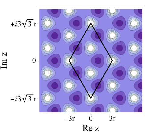
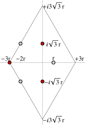
Figure 2: Left panel: The level plot shows $|f(z)|$ (56) on the complex plane $z$. Black rhombus depicts the fundamental domain of $f(z)$ around the origin. Right panel: Three poles (filled circles) and three zeroes (empty circles) of $f(z)$ in the complex plane $z$ inside the fundamental domain around the origin.

Within the fundamental domain (see Fig. 2) the function $f(z)$ possesses $3$ simple poles:

• a pole at $z=-3r$ with the residue $1$;

• a pole at $z=i\sqrt{3}r$ with the residue $e^{-\frac{2\pi i}{3}}$;

• a pole at $z=-i\sqrt{3}r$ with the residue $e^{\frac{2\pi i}{3}}$.

and $3$ zeros at $z=r$ and $z=-2r\pm i\sqrt{3}r$.

Quasi-renormalizable QFTs in which the result of LL-resummation is expressed through elliptic function look particularly appealing. The doubly periodic structure of the Landau poles may reflect the highly non-trivial properties of such theories. The physical examples of such theories are presented in Ref. [16].

4.5 A More General Form of the Recurrence Relation

In this subsection we consider a particular case of the recurrence relation (26) with arbitrary real parameters $A_{0}$, $A_{1}$ and $A_{2}=0$. Our interest in considering this example relies on the experience with the bissextile massless EFTs in $D=2$ [16]. This recurrence relation turns to be equivalent to the following non-linear differential functional equation for the generating function $f(z)$ (23):

$$f^{\prime}(z)=A_{0}f^{2}(z)+A_{1}f^{2}(-z);\ \ f(0)=1.$$ (67)

We introduce the symmetric and antisymmetric parts of $f(z)$:

$$u(z)=\frac{1}{2}\left(f(z)+f(-z)\right);\ \ \ v(z)=\frac{1}{2}\left(f(z)-f(-z)\right).$$ (68)

The equation (67) then turns to be equivalent to the following system of differential equations:

$$\begin{cases}u^{\prime}(z)=2(A_{0}-A_{1})u(z)v(z),\\ v^{\prime}(z)=(A_{0}+A_{1})(u^{2}(z)+v^{2}(z));\end{cases}\ \ \ u(0)=1;\ \ v(0)=0.$$ (69)

First we consider the case $A_{0}\neq A_{1}$, $A_{0}\neq-A_{1}$, $A_{0}\neq 3A_{1}$. One can check that the system of the differential equations (69) possesses the following first integral

$$\left(u^{2}(z)+\frac{3A_{1}-A_{0}}{A_{0}+A_{1}}v^{2}(z)\right)^{A_{0}-A_{1}}=u^{A_{0}+A_{1}}(z).$$ (70)

Expressing $v(z)$ from the first equation of (69) and substituting it into the first integral (70) we obtain the following non-linear differential equation for $u(z)$:

$$\frac{3A_{1}-A_{0}}{4(A_{0}+A_{1})(A_{0}-A_{1})^{2}}\left[u^{\prime}(z)\right]^{2}=u^{N(A_{0},A_{1})}(z)-u^{4}(z);\ \ \ u(0)=1,$$ (71)

where

$$N(A_{0},A_{1})=\frac{3A_{0}-A_{1}}{A_{0}-A_{1}}.$$ (72)

In the case $N(A_{0},A_{1})=0,\,\ldots,\,3$ the solution of (71) can be expressed through the elliptic functions (or their degeneracies). Below we present the summary of the corresponding solutions.

• In the case $N(A_{0},A_{1})=0\Leftrightarrow A_{1}=3A_{0}$ the solution of the equation (69) can be expressed as follows

  $$u(z)=\frac{\wp(z;\,-64A_{0}^{4},\,0)-4A_{0}^{2}}{\wp(z;\,-64A_{0}^{4},\,0)+4A_{0}^{2}};\ \ \ v(z)=-\frac{u^{\prime}(z)}{4A_{0}u(z)}=-\frac{2A_{0}\wp^{\prime}(z;\,-64A_{0}^{4},\,0)}{\wp^{2}(z;\,-64A_{0}^{4},\,0)-16A_{0}^{4}}$$

  through the Weierstraß $\wp$-function satisfying the master equation (62) with ${\rm g}_{2}=-64A_{0}^{4}$; ${\rm g}_{3}=0$.

• The case $N(A_{0},A_{1})=1\Leftrightarrow A_{0}=0$ corresponds to the generalization of (46) for arbitrary $A_{1}$. It is reduced to the former case for $A_{1}=-1$.

  The solution can be expressed through the Weierstraß $\wp$-function

  $$f(z)=\frac{18\wp^{2}(z;\,0,\,\frac{4A_{1}^{6}}{27})-9A_{1}\wp^{\prime}(z;\,0,\,\frac{4A_{1}^{6}}{27})-12A_{1}^{2}\wp(z;\,0,\,\frac{4A_{1}^{6}}{27})+2A_{1}^{4}}{2(3\wp(z;\,0,\,\frac{4A_{1}^{6}}{27})+2A_{1}^{2})(3\wp(z;\,0,\,\frac{4A_{1}^{6}}{27})-A_{1}^{2})}.$$ (74)

  The corresponding $\wp$-function satisfies the master equation (62) with ${\rm g}_{2}=0$; ${\rm g}_{3}=\frac{4A_{1}^{6}}{27}$. Note that (74) indeed reduces to (64) for $A_{1}=-1$.

• The case $N(A_{0},A_{1})=3\Leftrightarrow A_{1}=0$ corresponds to the renormalizable theory (30) with $b_{1}=A_{0}$.

We also present a short summary of solutions for the special cases $A_{0}=A_{1}$, $A_{0}=-A_{1}$, $A_{0}=3A_{1}$.

• The case $A_{0}=A_{1}$ results in the non-trivial solution in terms of the trigonometric functions:

  $$f(z)=1+\tan\left(2A_{0}z\right).$$ (75)

• The case $A_{0}=-A_{1}$ is trivial: $f(z)=1$.

• In the case $A_{0}=3A_{1}$ the first integral of the system (69) turns to be

  $$\log\left(u(z)\right)=\frac{v^{2}(z)}{2u^{2}(z)}.$$ (76)

  The equation for $u(z)$ reads

  $$\left[u^{\prime}(z)\right]^{2}=32A_{1}^{2}u^{4}(z)\log\left(u(z)\right);\ \ u(0)=1.$$ (77)

  The solution is therefore expressed in terms of the inverse of the Gauss error function

  $${\rm erf}(x)=\frac{2}{\sqrt{\pi}}\int_{0}^{x}dye^{-y^{2}}$$

  $$u(z)=e^{\left({\rm erf}^{-1}(4\sqrt{\frac{2}{\pi}}A_{1}z)\right)^{2}};\ \ \ v(z)=\frac{1}{4A_{1}}\frac{d}{dz}\left({\rm erf}^{-1}(4\sqrt{\frac{2}{\pi}}A_{1}z)\right)^{2}.$$ (78)

In order to work out the additional solutions of (71) it is instructive to perform the substitution

$$w(z)=\frac{1}{u(z)}.$$ (79)

The equation (71) transforms into

$$\frac{3A_{1}-A_{0}}{4(A_{0}+A_{1})(A_{0}-A_{1})^{2}}\left[w^{\prime}(z)\right]^{2}=w^{4-N(A_{0},A_{1})}(z)-1.$$ (80)

As is was already worked out, for $N(A_{0},A_{1})=0,\,1,\,2,\,3$ the solution is expressed in terms of elliptic functions (or their degeneracies). For negative integer $N(A_{0},A_{1})$ the solution will be expressed on terms of hyperelliptic functions (or their degeneracies).

Another useful substitution is

$$q(z)=\frac{1}{u^{2}(z)}.$$ (81)

The equation (71) then reads

$$\frac{3A_{1}-A_{0}}{4(A_{0}+A_{1})(A_{0}-A_{1})^{2}}\left[q^{\prime}(z)\right]^{2}=q^{3-\frac{N(A_{0},A_{1})}{2}}(z)-q(z).$$ (82)

Apart from the already studied cases, this equation possesses the additional elliptic solution for $N(A_{0},A_{1})=-2\Leftrightarrow A_{0}=\frac{3}{5};\;A_{1}=1$:

$$u(z)=\sqrt{\frac{75\wp\left(z;\,0,\,4\left(\frac{32}{75}\right)^{3}\right)-64}{75\wp\left(z;\,0,\,4\left(\frac{32}{75}\right)^{3}\right)+32}};$$

$$v(z)=-\frac{4500\wp^{\prime}\left(z;\,0,\,4\left(\frac{32}{75}\right)^{3}\right)}{(75\wp\left(z;\,0,\,4\left(\frac{32}{75}\right)^{3}\right)-64)(75\wp\left(z;\,0,\,4\left(\frac{32}{75}\right)^{3}\right)+32)}\,,$$ (83)

where $\wp\left(z;\,0,\,4\left(\frac{32}{75}\right)^{3}\right)$ satisfies the master equation (62) with ${\rm g}_{2}=0$; ${\rm g}_{3}=4\left(\frac{32}{75}\right)^{3}$.

5 Conclusions and Outlook

The summation of the leading logarithms in EFTs to all orders of loop expansion can provide us new valuable information on the structure of the perturbation theory expansion in EFTs and help to mirror the non-trivial properties of the general non-perturbative solution.

In this paper we address a class of non-linear recurrence equations that we believe is relevant for the QFT applications. These recurrence relations are equivalent to systems of non-linear differential equations for the corresponding generating functions. We point out the explicit solutions of these differential equations in terms of elliptic functions (and their degeneracies).

We introduce the concept of quasi-renormalizable field theories in which the generating function for the LL-coefficients is meromorphic and may contain an infinite number of the Landau poles. This can be seen as a generalization of the class of usual renormalizable QFTs in which the LL asymptotic behavior is controlled by the presence of a single Landau pole. The situation in which the LL asymptotic behavior of EFT is described by a (doubly)periodic function is particularly interesting. The periodic pole structure could have relation to the mass spectrum of the full theory. The explicit examples of quasi-renormalizable effective field theories in $D=2$ with an infinite number of periodically located Landau poles are presented in Ref. [16].

We also expect possible non-trivial connections between QFT and various branches of pure mathematics such as combinatorics, theory of continued fractions and theory of orthogonal polynomials.

References

- [1] A. N. Vasiliev, ‘‘The Field Theoretic Renormalization Group in Critical Behavior Theory and Stochastic Dynamics’’ (Chapman & Hall/ CRC, 2004).
- [2] G. Colangelo, Phys. Lett. B 350, 85 (1995), Erratum: [Phys. Lett. B 361, 234 (1995)] [hep-ph/9502285].
- [3] D. I. Kazakov, Theor. Math. Phys. 75, 440 (1988) [Teor. Mat. Fiz. 75, 157 (1988)].
- [4] M. Buchler and G. Colangelo, Eur. Phys. J. C 32, 427 (2003) [hep-ph/0309049].
- [5] M. Bissegger, and A. Fuhrer, Phys. Lett. B 646, 72 (2007) [hep-ph/0612096].
- [6] N. Kivel, M. V. Polyakov, and A. Vladimirov, Phys. Rev. Lett. 101, 262001 (2008) [arXiv:0809.3236 [hep-ph]].
- [7] J. Koschinski, M. V. Polyakov, and A. A. Vladimirov, Phys. Rev. D 82, 014014 (2010) [arXiv:1004.2197 [hep-ph]].
- [8] N. A. Kivel, M. V. Polyakov, and A. A. Vladimirov, JETP Lett. 89, 529 (2009) [arXiv:0904.3008 [hep-ph]].
-
[9]
A. A. Vladimirov,
Infrared Logarithms in Effective Field Theories, PhD thesis, Ruhr University, Bochum, 2010, unpublished
http://www-brs.ub.ruhr-uni-bochum.de/netahtml/HSS/Diss/VladimirovAlexey/diss.pdf. - [10] M. V. Polyakov, and A. A. Vladimirov, Theor. Math. Phys. 169, 1499 (2011) [arXiv:1012.4205 [hep-th]].
- [11] B. Ananthanarayan, S. Ghosh, A. Vladimirov, and D. Wyler, Eur. Phys. J. A 54, no. 7, 123 (2018) [arXiv:1803.07013 [hep-ph]].
- [12] I. A. Perevalova, M. V. Polyakov, A. N. Vall, and A. A. Vladimirov, ‘‘Chiral Inflation of the Pion Radius,’’ arXiv:1105.4990 [hep-ph].
- [13] J. Bijnens, and L. Carloni, Nucl. Phys. B 827, 237 (2010) [arXiv:0909.5086 [hep-ph]].
- [14] J. Bijnens, and L. Carloni, Nucl. Phys. B 843, 55 (2011) [arXiv:1008.3499 [hep-ph]].
- [15] J. Bijnens, and A. A. Vladimirov, Nucl. Phys. B 891, 700 (2015) [arXiv:1409.6127 [hep-ph]].
- [16] J. Linzen, M. V. Polyakov, K. M. Semenov-Tian-Shansky, and N. S. Sokolova, Exact Summation of Leading Infrared Logarithms in Effective Field Theories, under preparation.
- [17] L. D. Landau, A. A. Abrikosov, and I. M. Khalatnikov, Dokl. Akad. Nauk SSSR 95, 497, 773, 1177 (1954).
- [18] D. Malyshev, Phys. Lett. B 578, 231 (2004) [hep-th/0307301].
- [19] D. V. Malyshev, Theor. Math. Phys. 143, 505 (2005) [Teor. Mat. Fiz. 143, 22 (2005)] [hep-th/0408230].
- [20] D. Kreimer, Adv. Theor. Math. Phys. 2, 303 (1998) [q-alg/9707029].
- [21] A. T. Borlakov, D. I. Kazakov, D. M. Tolkachev, and D. E. Vlasenko, JHEP 1612, 154 (2016) [arXiv:1610.05549 [hep-th]].
- [22] D. I. Kazakov, and D. E. Vlasenko, Phys. Rev. D 95, no. 4, 045006 (2017) [arXiv:1603.05501 [hep-th]].
- [23] D. I. Kazakov, A. T. Borlakov, D. M. Tolkachev, and D. E. Vlasenko, Phys. Rev. D 97, no. 12, 125008 (2018) [arXiv:1712.04348 [hep-th]].
-
[24]
J. Koschinski,
Leading Logarithms
in Four Fermion Theories,
PhD thesis, Ruhr University, Bochum, 2015, unpublished
https://d-nb.info/1109051174/34. - [25] A. Hammerstein, Acta Math. 54, 117 (1930).
- [26] C. L. Dolph, Trans. Amer. Math. Soc., Vol. 66, 289 (1949).
- [27] N. J. A. Sloane, The On-Line Encyclopedia of Integer Sequences (OEIS) https://oeis.org/A000108.
- [28] A. A. Migdal, Annals Phys. 109, 365 (1977).
- [29] A. A. Migdal, Annals Phys. 110, 46 (1978).
- [30] A. A. Migdal, Meromorphization of Large QFT, arXiv:1109.1623 [hep-th].
- [31] A. A. Migdal, Integral Equation for CFT/String Duality, arXiv:1107.2370 [hep-th].
- [32] J. Erlich, G. D. Kribs and I. Low, Phys. Rev. D 73, 096001 (2006) [hep-th/0602110].
- [33] R. Bacher, and P. Flajolet, Ramanujan J 21, 71 (2010) [arXiv:0901.1379 [math]].
- [34] E. van Fossen Conrad, and P. Flajolet, Séminaire Lotharingien de Combinatoire, B54g, 1 (2006) [arXiv:math/0507268 [math.CO]].
- [35] N. J. A. Sloane, The On-Line Encyclopedia of Integer Sequences (OEIS) https://oeis.org/A098777.
- [36] A. C. Dixon, Quart. J. Math., 24, p. 167-233 (1890).
- [37] . . , << >>, 3, 2, << >>, , 1974 (in Russian).