Spatially resolved mass-to-light from the CALIFA survey

We investigated the mass-to-light versus color relations (MLCRs) derived from the spatially resolved star formation history (SFH) of a sample of 452 galaxies observed with integral field spectroscopy in the CALIFA survey. We derived the stellar mass ($M_{\star}$) and the stellar mass surface density ($\Sigma_{\star}$) from the combination of full spectral fitting (using different sets of stellar population models) with observed and synthetic colors in optical broad bands. This method allows obtaining the radial structure of the mass-to-light ratio ($M/L$) at several wavelengths and studying the spatially resolved MLCRs. Our sample covers a wide range of Hubble types from Sc to E, with stellar masses ranging from $M_{\star}\sim 10^{8.4}$ to $10^{12}$ M_⊙. The scatter in the MLCRs was studied as a function of morphology, stellar extinction, and emission line contribution to the colors. The effects of the initial mass function (IMF) and stellar population models in the MLCRs were also explored. Our main results are that (a) the $M/L$ ratio has a negative radial gradient that is steeper within the central 1 half-light-radius (HLR). It is steeper in Sb-Sbc than in early-type galaxies. (b) The MLCRs between $M/L$ and optical colors were derived with a scatter of $\sim$ 0.1 dex. The smallest dispersion was found for the combinations ($i$, $g-r$) and ($R$, $B-R$). Extinction and emission line contributions do not affect the scatter of these relations. Morphology does not produce a significant effect, except if the general relation is used for galaxies redder than $(u-i)>4$ or bluer than $(u-i)<0$. (c) The IMF has a large effect on MLCRs, as expected. The change from a Chabrier to a Salpeter IMF produces a median shift of $\sim$ 0.29 dex when mass loss from stellar evolution is also taken into account. (d) These MLCRs are in agreement with previous results, in particular for relations with $g$ and $r$ bands and the $B$ and $V$ Johnson systems.

1 Introduction

During the past decade, large-scale surveys of galaxies such as the Sloan Digital Sky Survey (SDSS, Stoughton et al. (2002)) or the Galaxy And Mass Assembly (GAMA, Driver et al. (2011)) survey, have shown that sorting galaxies by their stellar mass ($M_{\star}$) is a useful way to classify them. This is so because the stellar mass is strongly correlated with other global galaxy properties such as the stellar mass surface density ($\Sigma_{\star}$) (Kauffmann et al. 2003b, a), age, and metallicity of the stellar populations (Gallazzi et al. 2005; Cid Fernandes et al. 2005; Gallazzi et al. 2006; Mateus et al. 2006; Asari et al. 2007), and with the star formation rate (SFR) (Brinchmann et al. 2004). The correlations and the scatter of these global relations can be understood as a sequence on mass where the position of each galaxy is a consequence of their mass growth assembly history and its evolutionary state (e.g., Behroozi et al. 2013).

Other works based on spatially resolved data have shown that $\Sigma_{\star}$ is a fundamental parameter that drives the star formation history (SFH) of galaxies (Bell & de Jong 2000). More recently, integral field spectroscopic surveys have found local relations between $\Sigma_{\star}$ and local stellar ($Z_{\star}$, González Delgado et al. 2014a) and gas metallicity (Sánchez et al. 2013), the age of the stellar populations (González Delgado et al. 2014b; Goddard et al. 2017; Scott et al. 2017), and the star formation rate (González Delgado et al. 2016; Cano-Díaz et al. 2016). These local relations are similar to the global ones, implying that $\Sigma_{\star}$ regulates the star formation in disks, while $M_{\star}$ drives the star formation in the spheroidal components.

$M_{\star}$ and $\Sigma_{\star}$ are thus important properties of galaxies that cannot be measured directly. Deriving these quantities from observed data involves stellar populations synthesis (SPS) models. The relation between light and mass can be obtained by modeling the following three properties:

• The galaxy spectrum by fitting its stellar continuum with a combination of single stellar population models (e.g., Panter et al. 2003; Cid Fernandes et al. 2005; Tojeiro et al. 2011; Pérez et al. 2013; Sánchez et al. 2016b; García-Benito et al. 2017), or selected spectral indices with a library of models of parametric SFHs (e.g., Kauffmann et al. 2003b; Gallazzi et al. 2005; López Fernández et al. 2016, 2018).

• The galaxy spectral energy distribution from optical-to-near-IR (NIR) broadband photometry, usually with a library of parametric SFHs (e.g., Taylor et al. 2011; see Walcher et al. 2011 and Conroy (2013) for reviews).

• The relation between colors and the mass-to-light ratio at some wavelength:

  $$\log{M/L_{\lambda_{i}}}=a_{\lambda_{i}}+b_{\lambda_{i}}\times(m_{\lambda_{j}}-m_{\lambda_{k}}),$$ (1)

  where the bands $\lambda_{i}$, $\lambda_{j}$, and $\lambda_{k}$ may be independent, or $\lambda_{i}$ = $\lambda_{j}$ or $\lambda_{k}$ (Bell & de Jong 2001; Bell et al. 2003; Zibetti et al. 2009; Gallazzi & Bell 2009; Taylor et al. 2011; Into & Portinari 2013; McGaugh & Schombert 2014; Roediger & Courteau 2015).

Certainly, the $\rm{M/L_{\lambda}}$-color relation (MLCR) is the simplest method to derive $M_{\star}$ (and $\Sigma_{\star}$), as it relies on photometry in only two bands. However, the uncertainty in mass is usually larger with MLCR than with the other two methods, and it depends on the SFH, the initial mass function (IMF), and the extinction assumed to model the MLCR (Conroy 2013).

In their pioneering work, Bell & de Jong (2001) found that along the SFH (parametrized by a $\tau$ model), galaxies move across a well-defined locus in the space of $M/L_{B}$ versus $B-R$, suggesting that the $B-R$ color is a good proxy for $M/L_{B}$. In a more recent work, using an extensive library of SFHs and the stellar masses derived by SED fitting of the SDSS bands for the GAMA survey, Taylor et al. (2011) found that their calibration $M/L_{i}$ versus $(g-i)$ color can be used to estimate $M_{\star}$ with an accuracy of $\leq$ 0.1 dex. Another important conclusion from their work is that the age-metallicity-dust degeneracy helps in the estimation of $M/L_{i}$ because it moves the galaxies along the $M/L_{i}$ versus $(g-i)$ relation.

From stellar population synthesis models, the amplitude of the evolution of $M/L$ is much less pronounced in the NIR than at optical wavelengths (Leitherer et al. 1999; Bruzual & Charlot 2003). Recent works based on Spitzer data use a constant value of $\sim 0.5$ M_⊙/L_⊙ to convert the 3.6$\mu$m emission into $M_{\star}$ (McGaugh & Schombert 2014). Other studies found that $M/L_{3.6\mu m}$ also depends on the $[3.6]-[4.5]$ color (Meidt et al. 2012), and this color may be contaminated by non-stellar sources (Querejeta et al. 2015). Furthermore, modeling the asymptotic giant branch phase of stellar evolution is crucial in population synthesis models (Into & Portinari 2013), and it may have a major impact on $M/L$ at NIR wavelengths.

Most previous works to date have obtained MLCR based on the integrated $M/L_{\lambda}$ (Bell et al. 2003; Gallazzi & Bell 2009; Taylor et al. 2011; Into & Portinari 2013; Roediger & Courteau 2015). However, galaxies have $M/L_{\lambda}$ and color gradients, and the effects of spatial variations of the SFH, extinction, metallicity, and age on the MLCR have not been explored before. This is the goal of this work. We use the full spectral synthesis technique by fitting the spatially resolved optical spectroscopy provided by the CALIFA survey to obtain the spatially resolved $M/L$, retrieving for each spaxel in the galaxy the SFH (as in González Delgado et al. 2017), the stellar extinction, metallicity, and ages (as in González Delgado et al. 2015), the recent SFR (as in González Delgado et al. 2016), and $\Sigma_{\star}$ (as in González Delgado et al. 2014b). Optical colors are measured on the observed spectra and on the synthetic ones to explore the effect from the emission lines on the colors in the MLCR. Because the CALIFA sample covers all Hubble types, we are able to explore the radial profiles of $M/L_{\lambda}$ and their gradient with galaxy morphology, and their effect on the MLCR.

This paper is organized as follows. Section 2 describes the observations and the properties of the galaxies analyzed here. Section 3 explains the analysis method for retrieving the spatially resolved SFH and $\Sigma_{\star}$, and how colors are measured. Section 4 presents the radial profiles of $M/L$. In Section 5 we derive the MLCRs and compare these results with those from the literature. Section 7 reviews our main findings.

Throughout this work we assume a flat $\Lambda$CDM cosmology with $\Omega_{M}$ = 0.3, $\Omega_{\Lambda}$ = 0.7, and H₀ = 70 km s^-1 Mpc^-1.

2 Sample and data

2.1 Sample

The sample was selected from the final CALIFA data release (Sánchez et al. 2016a, hereafter DR3), with a total 646 galaxies observed with the V500 grating, 484 with the V1200 grating, and 446 galaxies with the COMB setup (the combination of the cubes from both setups). The DR3 release is the combination of two samples: a) the CALIFA main sample (MS) consists of galaxies belonging to the CALIFA mother sample, with a total of 529 observed with V500 and 396 with the COMB, all included in the DR3; b) the rest of the galaxies belong to the CALIFA extension sample, a set of galaxies observed within the CALIFA collaboration as part of different ancillary science projects (see DR3).

The CALIFA mother sample is fully described in Walcher et al. (2014). The main properties of this sample are (a) an angular isophotal diameter between $45{\tt{}^{\prime\prime}}$ and $79{\tt{}^{\prime\prime}}$; (b) a redshift range $0.005\leq z\leq 0.03$; and (c) color ($u-r<5$) and magnitude ($-24<M_{r}<-17$), thus covering the whole color-magnitude diagram. The sample is not limited in volume, but it can be ”volume-corrected”, allowing us to provide estimates of the stellar mass function (Walcher et al. 2014) and other cosmological observables such as $\rho_{\rm SFR}$ (González Delgado et al. 2016; López Fernández et al. 2016, 2018) and $\rho_{\star}$.

The mother and extended CALIFA samples were morphological classified through visual inspection of the SDSS $r$-band images. As in our previous works (e.g., González Delgado et al. 2016; García-Benito et al. 2017), we grouped the galaxies into seven morphological bins: E (65 galaxies), S0 (54, including S0 and S0a), Sa (70, including Sa and Sab), Sb (75), Sbc (76), Sc (77, including Sc and Scd), and Sd (35, including Sd, Sm, and Irr).

2.2 Data

Observations were carried out at the 3.5m telescope at Calar Alto observatory with the Postdam Multi Aperture Spectrograph (PMAS, Roth et al. 2005) in the PPaK mode (Verheijen et al. 2004), created for the Disk Mass Survey project (Bershady et al. 2010). PPak contains a bundle of 331 science fibers of 2.7″ diameter each and a 71″$\times$ 64″ field of view (FoV; Kelz et al. 2006). The observations were planed to observe each galaxy with two different overlapping setups. Here, we analyze only the low-resolution setup (COMB; R$\sim$850) that covers from 3745 Å to 7500 Å with a spectral resolution of $\sim$ 6 Å full width at half-maximum (FWHM). The spatial sampling of the data cubes is 1″/spaxel with a point spread function (PSF) of FWHM $\sim$ 2.6″, which at the mean redshift of the sample corresponds to a physical resolution of $\sim$ 0.7 kpc. The data were calibrated with version V2.2 of the reduction pipeline (Sánchez et al. 2016a). Details about the observational strategy and data processing are given in Sánchez et al. (2012), Husemann et al. (2013), García-Benito et al. (2015), and Sánchez et al. (2016a).

3 Method: 2D maps of stellar mass, colors, and M/L_λ

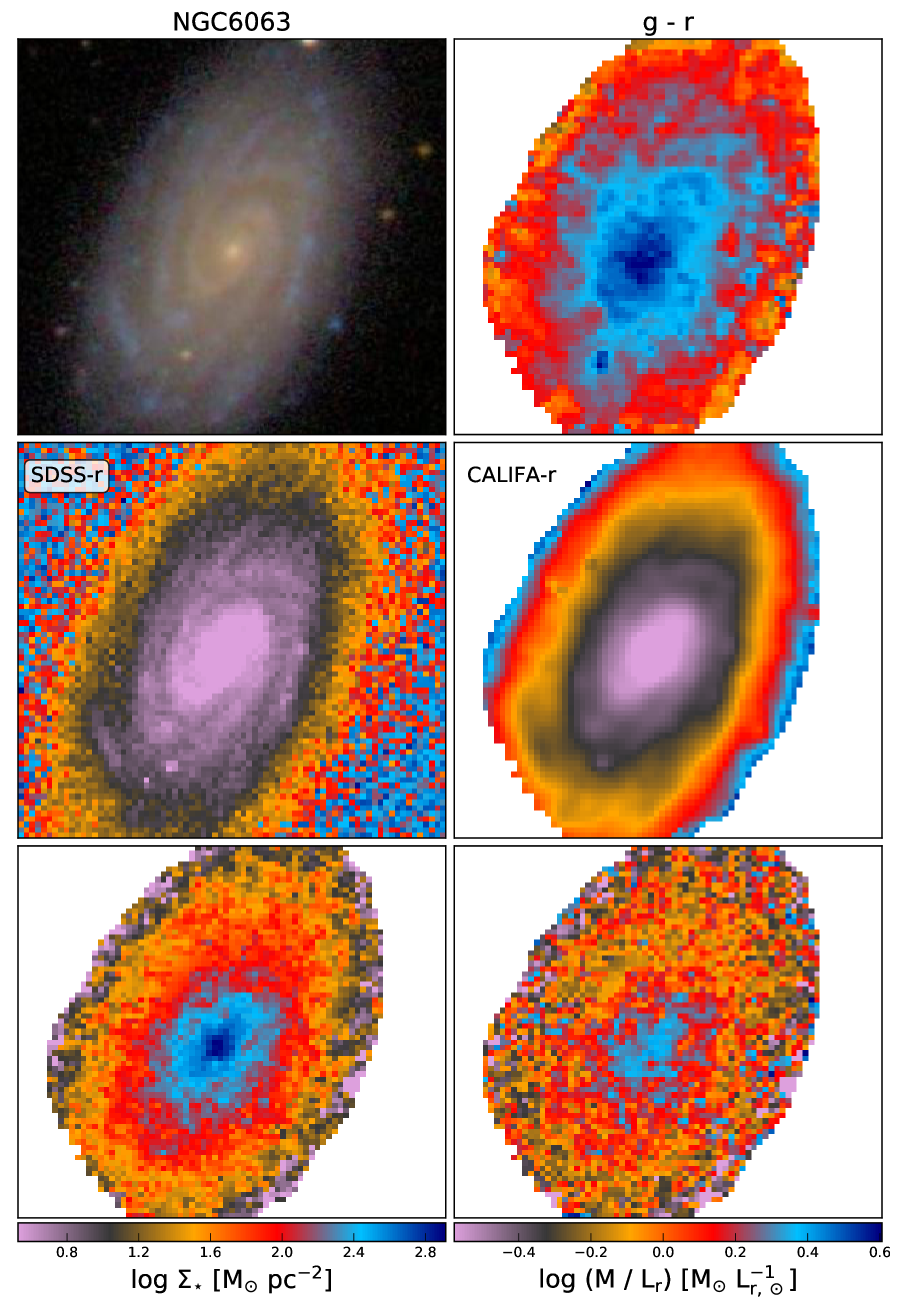
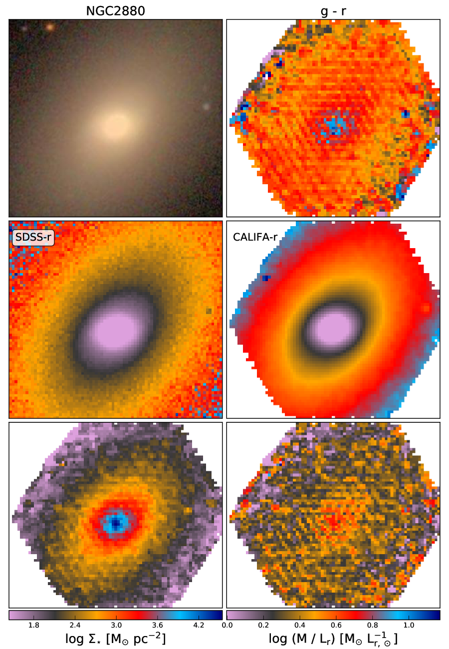
Figure 1: Examples of some of the data products used in the analysis of this work. 2D maps obtained from the CALIFA data cubes for NGC 6063 (unbarred Sbc, left) and NGC 2880 (E7, right). For each galaxy, the figure shows maps of $g-r$ (upper right), $r$ band (middle right), $\Sigma_{\star}$ (lower left), and $\rm M/L_{r}$ (lower right). For the sake of comparison, a three-color postage-stamp SDSS image (upper left) and an SDSS $r$ band (middle left) reprojected to the same pixel scale as the CALIFA data cubes are also shown.

3.1 Spatially resolved SFH

For this work, we obtained the spatially resolved SFH of each galaxy to derive the stellar mass surface density ($\Sigma_{\star}$) and $M_{\star}$. We followed the same method as in previous works (e.g., Pérez et al. 2013, González Delgado et al. 2014b, González Delgado et al. 2015). In short, we fit with starlight (Cid Fernandes et al. 2005) the spectrum of each individual spaxel (pixelwise) within the isophote level where the average signal-to-noise ratio (S/N) $\geq$ 3, decomposing the spectra in terms of stellar populations with different ages and metallicities.

We used base CBe, a set of 246 SSPs from an updated version of Bruzual & Charlot (2003, hereafter BC03) models (Charlot & Bruzual 2007, hereafter CB07; private communication). In CB07, the spectral library STELIB (Le Borgne et al. 2003) is replaced by a combination of the MILES (Sánchez-Blázquez et al. 2006; Falcón-Barroso et al. 2011) and granada (Martins et al. 2005) libraries. The evolutionary tracks are those collectively known as Padova 1994 (Alongi et al. 1993; Bressan et al. 1993; Fagotto et al. 1994a, b; Girardi et al. 1996). The metallicity covers $\log Z_{\star}/Z_{\odot}=-2.3$, $-1.7$, $-0.7$, $-0.4$, 0, and $+0.4$, while ages run from 1 Myr to 14 Gyr. The IMF is that of Chabrier (2003). Dust effects were modeled as a foreground screen with a Cardelli et al. (1989) reddening law with R_V = 3.1.

MILES and STELIB differ in a number of ways. MILES has a larger number of stars and a wider range in stellar parameters (effective temperature, gravity, and metallicity; see Sánchez-Blázquez et al. 2006). While both MILES and STELIB have only few massive stars, in our analysis MILES is complemented with the synthetic stellar library GRANADA (Martins et al. 2005) and the SSP templates by González Delgado et al. (2005). Although the stellar metallicity in galaxies is a parameter that always has a large uncertainty, several works indicate that results are more consistent for the same data fitted with MILES + GRANADA than with STELIB; for example, for CALIFA data sets (e.g. Fig.9 in Cid Fernandes et al. 2014) or for LMC and SMC stellar clusters (González Delgado & Cid Fernandes 2010).

The results were then processed through pycasso (the Python CALIFA starlight Synthesis Organizer; Cid Fernandes et al. 2013; de Amorim et al. 2017) to produce a suite of spatially resolved stellar population properties. pycasso organizes the information into a multi-dimensional data structure with spatial as well as age and metallicity dimensions. From these, 2D maps of stellar mass surface density, $\Sigma_{\star}$, stellar extinction (A_V), and luminosity surface density were obtained to derive 2D maps and radial profiles of M/L.

3.2 2D maps of stellar mass

For each spectrum, the stellar mass was derived from starlight as explained in Cid Fernandes et al. (2013). To reflect the mass currently in stars, the initial mass formed in stars is corrected for the mass returned to the interstellar medium during stellar evolution. These results were then processed through pycasso to produce 2D maps of the stellar mass distribution. The galaxy’s total stellar mass was obtained by adding the masses of individual spaxels. This method takes into account the spatial variations of the SFH and extinction across the face of the galaxy. We also take into account areas that were masked in the data cube, replacing the missing spaxels by the average values at the same radial distance.

Masses obtained with base CBe are on average 0.29 dex lower than those used in García-Benito et al. (2017). This is the factor expected due to change of the IMF from Chabrier to Salpeter. Throughout this paper all the stellar masses used in the M/L and MLCR (either in 2D maps or profiles) come from these starlight results, unless explicitly stated otherwise.

3.3 Optical images and colors

We computed colors in two alternative ways: 1) the CALIFA data cubes were convolved with the SDSS $g$ and $r$ and the Johnson $B$ and $V$ filter responses. The label Obs was attached to results that were computed using these data; 2) synthetic data cubes were computed by assigning to each spaxel the corresponding synthetic spectrum derived from the full spectral fit. These synthetic data cubes were convolved with all the filters available within the wavelength range, generating images in the $u,g,r,i,z$ SDSS bands and the $B$, $V$, $R$ Johnson bands. The label Syn was attached to results that were computed using these data.

The two methods allow us to estimate the variations of the MLCRs that are due to the effect of stellar extinction and the contribution from emission lines. Furthermore, when the synthetic spectra are used, the second method provides images in optical bands at wavelengths that are not covered by our observations. We derived both restframe and observed colors for each galaxy. However, because our galaxies are in a very small range of redshift, the difference is very small, $\sim$ 0.01 magnitudes. In what follows, all results are calculated in restframe unless noted otherwise.

Since starlight provides the stellar extinction, the luminosity (and colors) in the M/L (and therefore in the MLCR) can be given as not dereddened (M/L_λ) or as dereddened quantities (M/L${}^{Dered}_{\lambda}$). In this work, all luminosity and color values are given uncorrected for reddening, unless otherwise specified. Obviously, the mass is the same in both cases.

3.4 2D maps of M/L_λ

For each galaxy, the image of M/L_λ was obtained by dividing the 2D map of stellar mass by the image in $L_{\lambda}$, where $\lambda$ can be any of the optical SDSS bands or the $BVR$ Johnson bands. Figure 1 shows examples of the images obtained for two different galaxies. To the left, NGC 6063: $g-r$ color obtained with method (2) and ${\rm M/L_{r}}$. The SDSS three-color postage-stamp image is also shown. NGC 6063 (CALIFA 823) is an isolated unbarred Sbc galaxy (Walcher et al. 2014). The stellar mass map shows a clear radial variation from the inner to the outer parts of the galaxy, with a more pronounced gradient in the inner HLR and smoother profile in the outer one. This is also reflected in the $\rm M/L_{r}$ map. This behavior is typical of Sbc galaxies (see Fig. 2).

Figure 1 (right) shows the example for NGC 2880 (CALIFA 272), an isolated E7 galaxy. The color distribution is more homogeneous in this case, as expected for this type of galaxy. The mass map gradient is clearly more pronounced. The $\rm M/L_{r}$ map is smoother than for NGC 6063, but a gradient is still present, as seen in Fig. 2.

2D maps of $M/L_{\lambda}$ for each galaxy, together with the average radial profiles and MLCRs (see section 5), are available in http://pycasso.iaa.es/ML. Our magnitudes in the SDSS bands are given in the $AB$ system (Oke & Gunn 1983), while the Johnson $BVR$ are Vega magnitudes. The $M/L_{\lambda}$ is given in solar units, and it can be transformed from $M_{\odot}$/$L_{\odot}$ to $M_{\odot}$/ erg s^-1 Hz^-1 by adding 2.05, 1.90, and 1.81 to $\log{\rm M/L_{\lambda}}$ for $\lambda$ = $g$, $r$, and $i$, respectively.

4 Radial structure of the mass-to-light ratio

This section presents a series of results derived from the spatially resolved $M/L_{\lambda}$, including the radial structure of $M/L_{\lambda}$ and the radial gradients as a function of the galaxy morphology and galaxy mass. For each galaxy, the radial variation of $M/L_{\lambda}$ was obtained by compressing each individual 2D map in azimuthally averaged radial profiles. As in our previous studies (e.g., González Delgado et al. 2014b, 2015; García-Benito et al. 2017), the radial distance is expressed in units of the galaxy’s half-light-radius (HLR), a convenient metric when averaging radial information for different galaxies. The HLR is defined as the semi-major length of the elliptical aperture in the data cube that contains 50$\%$ of the luminosity at 5635 Å. To obtain the radial profile, we used elliptical apertures of thickness 0.1 HLR. The ellipticity and position angle were derived from the moments of the 5635 Å flux image of the data cube. Similarly using the mass, we define the half-mass-radius (HMR) as the semi-major length of the elliptical aperture that contains 50$\%$ of the mass.

4.1 Radial profiles

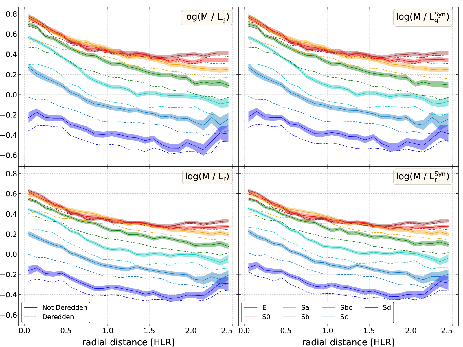
Figure 2: Radial profile of M/L for $g$ band (upper panels) and $r$ band (lower panels) stacked by Hubble type for the observed (left panels) and synthetic restframe spectra (right panels). The profiles with intrinsic extinction are shown in continuous lines and the deredden profiles (using the extinction values given by the stellar population analysis) in dashed lines. For the sake of clarity, the uncertainty band is plotted only in the not dereddened profiles.

Figure 2 shows azimuthally averaged radial profiles of $\rm M/L_{g}$ and $\rm M/L_{r}$. Results are stacked by Hubble type in seven morphological classes. In the left panels, the profiles are obtained from the observed spectrum, both not dereddened (continuous lines) and dereddened (dashed lines), using the results from the stellar population fitting. In the right panels we use the M/L_λ images obtained from the synthetic spectra, also corrected and not corrected for stellar extinction.

All profiles decrease outward, with inner regions having higher M/L. The profiles scale with the Hubble type. At any given distance, M/L is higher for early-type galaxies than for late-type spirals. Taking as reference the value at 1 HLR, the logarithmic value of $\rm M/L_{g}$ ($\rm M/L_{r}$) ranges from $-0.39$ ($-0.32$) to 0.42 (0.32) for Sd to E galaxies. The effect of the extinction is clearly seen in Fig. 2. This effect is more significant in the central regions of intermediate-type spirals, in particular in Sb/Sbc, where the value of the extinction and its central gradient is higher (González Delgado et al. 2015).

The effect of emission lines in M/L is very small, as can be seen from the comparison between observed and synthetic profiles in Fig. 2. For $\rm M/L_{g}$ ($\rm M/L_{r}$), the maximum difference is around 0.01 dex (0.02 dex) for late-type spirals.

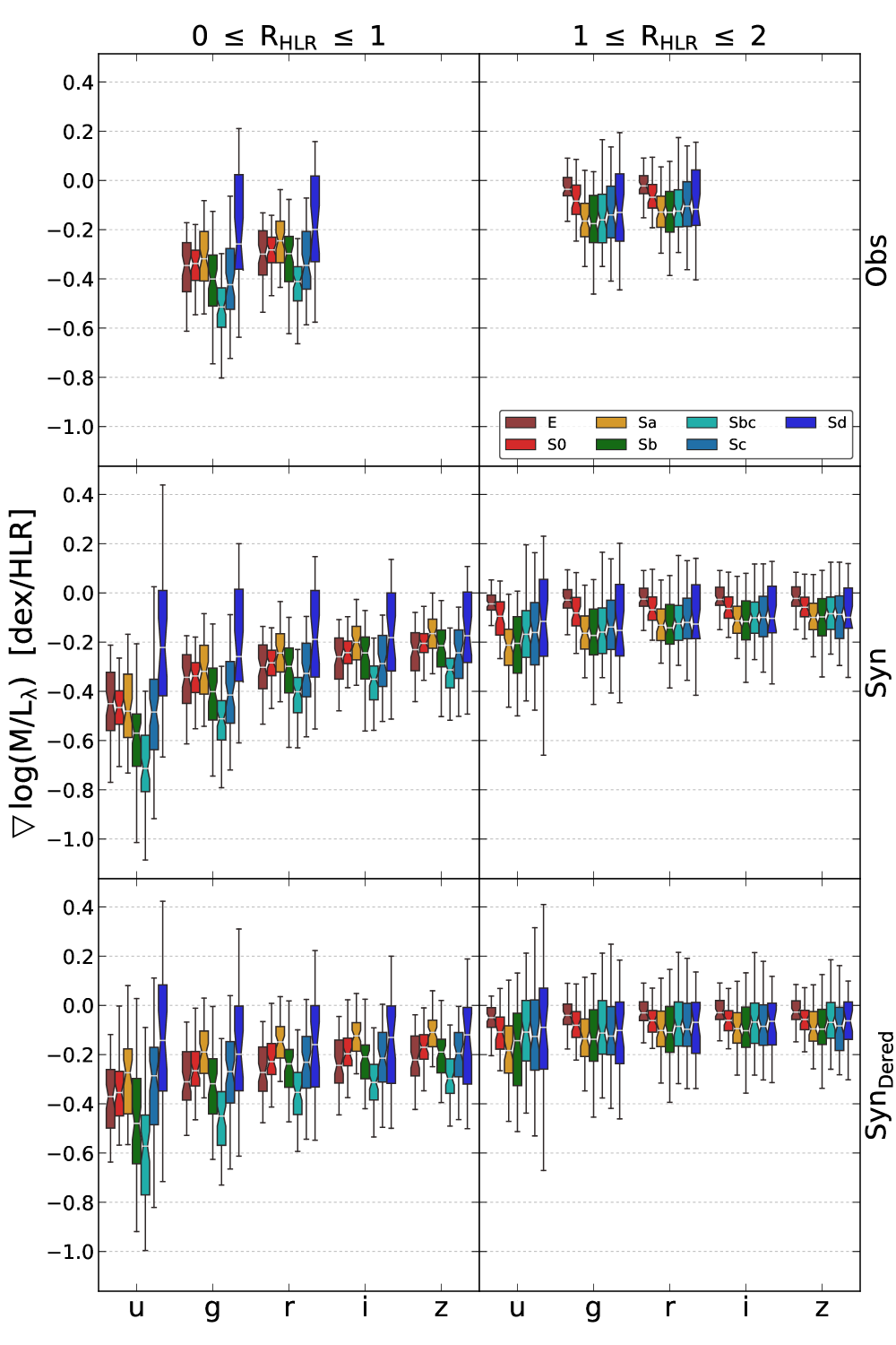
Figure 3: Box plot diagrams of the radial gradients of M/L_λ measured in the inner $\bigtriangledown_{in}$ (0 $\leq$ HLR $\leq$ 1; left panels) and outer $\bigtriangledown_{out}$ (1 $\leq$ HLR $\leq$ 2; right panels) spatial regions in the observed spectra (upper panels; Obs), synthetic spectra (middle panels; Syn), and dereddened synthetic spectra (lower panels; Syn_Dered).

4.2 Radial gradients

We can analyze Fig. 2 in another way. As in García-Benito et al. (2017), we performed a robust linear fit of the log M/L_λ profile over a radial range. We defined an inner radial gradient as the slope of the robust linear fit over the entire inner 1 HLR ($\bigtriangledown_{in}$) and in a similar way to the outer (1 $\leq$ HLR$\leq$ 2) radial gradient ($\bigtriangledown_{out}$). Expressed in this way, the gradients have units of dex/HLR.

Figure 3 presents box plot diagrams of the radial gradients of M/L_λ in these two spatial regions, measured in the observed (upper panels; $\rm M/L^{Obs}$), in the synthetic spectra (middle panels; $\rm M/L^{Syn}$), and in the dereddened syntetic spectra (lower panels; $\rm M/L^{Syn}_{Dered}$) for the SDSS bands. All of them show negative gradients, although their values are higher in the inner than in the outer regions. As mentioned in Sect. 4.1, the difference between synthetic and observed profiles is very small, which is also reflected in their gradients (for the filters in common).

There are two clear trends. The first is seen in the values of the gradient for a given filter as function of Hubble type. For the inner regions, the median value of the gradients of early-type galaxies (E, S0, Sa) displays a similar value. The gradient for spiral galaxies (Sb, Sba, Sc) decreases (more negative) to the minimum, shown by Sbc galaxies. Finally, the gradient rises again up to Sd galaxies, which have less steep slopes and the highest dispersion in their values, mimicking the HMR/HLR relation found in González Delgado et al. (2015) and García-Benito et al. (2017). The scatter is similar for early and intermediate types, but it is larger for late types. The behavior is slightly different for the outer regions. The slope is almost flat for E galaxies, with more negative values up to Sa galaxies, whereas the median value of the slope is almost constant for late-type galaxies.

The second trend can be appreciated by comparing the gradients obtained with different filters. In the inner regions, blue filters have more negative slopes than red filters, while in the outer regions the values are almost the same, with nearly no dependence on the filter. The scatter is in general lower for the outer regions, and blue filters (particularly $u$ and $g$) present a larger scatter than the remaining filters. In general, the outer regions show flatter (gradients) profiles than the inner regions.

It is worth noting that the gradients estimated using dereddened luminosities ($Syn_{Dered}$) present the same relative trends as the not dereddened values ($Syn$). The only difference lies in the absolute values, which show slightly flattened gradients for the dereddened luminosities.

5 Spatially resolved MLCRs

Several factors determine the position of a galaxy on the color-M/L diagram: metallicity, reddening, and SFH. In addition, these properties are expected to vary from place to place within a particular object and in different degrees depending on the type of galaxy. If the MLCRs are calibrated based on models, these have to take into account all the possible variations of the variables involved. The same argument can be applied to observational data: the underlying sample has to cover the full parameter space. We remark that the CALIFA sample selection allows the MLCRs to be calibrated with an homogeneous and complete sample of galaxies with spatially resolved data.

Since our methodology provides the radial profile of any magnitude (mass, luminosity, magnitudes, colors, etc.) as described in Sect. 4, it is fairly straightforward to compute the linear relations of log(M/L)-color quantities. We limit the spatial extension of our fits to 0 $\leq$ R_HLR $\leq$ 2. Unlike many integrated relations found in the literature, we are computing spatially resolved MLCRs. The CALIFA dataset allows us to compute MLCRs for the whole sample and for different subsets, grouped by Hubble types.

Tables 1, 2, 3, 4, LABEL:tb:hubtyp_SynR_AB_px1, and 5 present the slope, origin (following equation 1), and scatter of the linear log(M/L)-color relations for each filter combination, both for SDSS ($ugriz$; Tables 1, 3, LABEL:tb:hubtyp_SynR_AB_px1) and Johnson-Cousin bands ($BVR$; Tables 2, 4, 5). All are computed in restframe in the not dereddened synthetic spectra with base CBe and Chabrier IMF. The monochromatic mass-to-light ratios $(M/L_{\lambda})$ are in solar units. The SDSS $ugriz$ filters are in the AB magnitude system and the Johnson-Cousins $BVR$ filters are in the Vega magnitude system. $\sigma_{\lambda}$ is the scatter of the residuals of the relation log(M/L)-color.

We have computed the MLCRs for different types of samples and subsamples: 1) the whole sample comprising all 452 galaxies (Tables 1, 2); 2) subsamples of early- (E, S0, Sa), intermediate- (Sb, Sbc), and late-type (Sc, Sd) galaxies (Tables 3, and 4); and 3) grouped by Hubble type (Tables LABEL:tb:hubtyp_SynR_AB_px1 and 5).

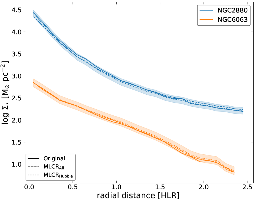
Figure 4: Comparison of radial profiles of $\Sigma_{\star}$: the original profile estimated from the stellar population results (continuous line), the profile derived from our MLCRs calibrated using all galaxies (dashed line), and the MLCRs by Hubble type (dotted line), for NGC 6063 and NGC 2880 (same galaxies as in Fig. 1). The $\Sigma_{\star}$ profiles derived from the MLCRs have been obtained from the $g-r$ 2D color map and the L_g 2D map. For the sake of clarity, only the uncertainty band from the Hubble type MLCR has been plotted (the others are on the same order).

Since these relations have been computed using spatially resolved data, it is possible to reproduce profiles just by using colors maps. Figure 4 compares the $\Sigma_{\star}$ radial profile obtained from the stellar population results (continuous line) and those derived using our MLCRs for galaxies NGC 6063 and NGC 2880 (same objects as in Fig. 1). The latter profiles have been computed from the $g-r$ 2D color and L_g maps using the MLCR calibrated using all galaxies (dashed line) and the Hubble-type relations (dotted line). It is clear from the plot that the profiles are very close to the originals within the errors. It is worth saying that these relations should be used only for evolved galaxies (galaxies at low redshift). At high redshift the trends might depart from the correlations since the age-metallicity relation could be different because the stellar populations would be younger. García-Benito et al. (2017) showed that 80% of the mass of the galaxies was already formed more than 10 Gyr ago (redshift $\sim$ 1.6), so that beyond this redshift limit the correlations might not be valid.

Appendix 5 includes the MLRCs using intrinsic luminosites, that is, using the dereddened synthetic spectra. These tables may be useful for comparison with models or simulations.

5.1 Uncertainties on MLCRs

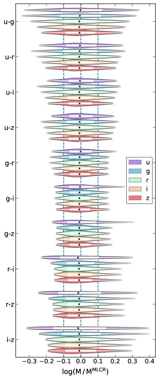
Figure 5: Violin plots of the difference between the spatially resolved mass obtained by applying our MLCRs and the mass derived from the stellar population fitting (Sect. 3.2) for the whole sample and all Sloan filter combinations. The corresponding box plot showing the interquartile range is plotted inside each violin plot. The inner dot in the box plot represents the median of the distribution.

We can assess the uncertainty on the derivation of M/L by estimating the scatter of the residuals of our $\rm{M/L_{\lambda}}$-color relations to the linear fit. In Tables 1, 2, 3, 4, LABEL:tb:hubtyp_SynR_AB_px1, and 5 we present the slope, origin, and scatter of the fits for each filter combination. The scatter estimates the error in the final calculation of the mass. The mean scatter using all filter combinations is $\sim$ 0.13 dex. The minimum scatter corresponds to the pairs ($i$, $g-i$), ($i$, $g-r$), ($r$, $g-i$), and ($R$, $B-R$), all with a value lower than 0.1 dex. The user can explore the tables to find the most suitable filter combination according to the type of galaxy.

To check the validity of our results and the estimated values of their uncertainties, we used these MLCRs to compute the mass for all our spatially resolved data (radial values) for the whole sample. From the measured colors (3.3), we obtained the M/L ratio and then we multiplied this value by the corresponding luminosity value (Sect. 3.4). Then, we computed the logarithmic difference between the masses from our stellar population fittings (M_⋆, Sect. 3.2) and the masses derived from the MLCRs (M${}^{MLCR}_{\star}$). The violin plots of the distribution of these residuals are shown in Fig. 5 for all Sloan filter combinations. The standard deviation of these distributions is an estimate of the uncertainties of the mass from the MLCRs. The values are almost equal to the scatter given in our tables. As expected, the distribution of the differences are centered around zero and it is easy to spot the combinations with less scatter.

5.2 Effect of extinction

In Fig. 2 the effect of the extinction in the radial profiles is clearly appreciated. We examine now the behavior of extinction in the log(M/L)-color plane. To better understand the position of galaxies in this space, we have computed the color ($g-r$) and $\rm M/L_{r}$ of all SSPs of our CBe base. Figure 6 shows the path of equal metallicity SSPs with age (the thicker the line, the older the age). We also show our sample distribution in gray contours encompassing 95% of the points. The reddening vector is also shown. All tracks move very quickly and appear hectic during the first few million years. After 10 Myr the tracks stabilize and follow a smoother path with some small changes at several points. Clearly, our distribution lies in the loci of intermediate to old age and medium to high metallicity unextincted tracks. Of course, younger ages of the same metallicities or lower metallicities can fall in the distribution area with different amounts of extinction, following the reddening vector.

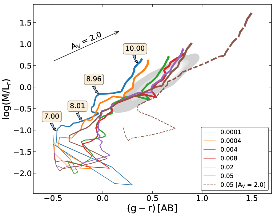
Figure 6: Tracks of the SSPs of the CBe base in the ${\rm log(M/L_{r}})-(g-r)$ plane. The library contains 6 metallicities and 41 ages. The tracks increase their line width with age (the older the age, the thicker the line). Four signposts mark the position and value of the (logarithmic) age in the lowest metallicity track. The highest metallicity track reddened by A_V = 2 mag together with a reddening vector of this amount are also shown. The density distribution of our sample is underlaid in gray contours encompassing 95% of the points.

Figure 7 shows the log(M/L)-color plane for some representative filter combinations. The contours follow the density distribution of the whole sample (encompassing 20% and 90% of the points) both for the not dereddened (observed, the one provided in the tables) and dereddened colors and luminosities. The best linear fits for both distributions are also shown. As can be appreciated, the MLCRs do not change in a significant manner with extinction. The contours cover a similar area and location in the plane. A clear effect of the extinction is to distribute points along the linear relation, as seen by the 20% contours.

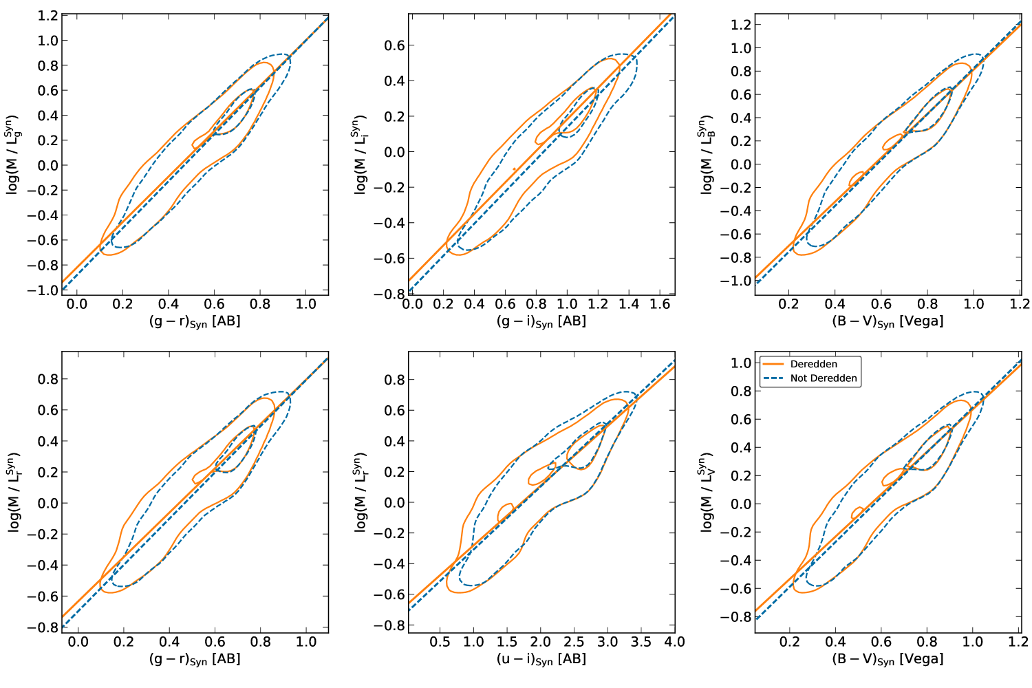
Figure 7: Relation between restframe color and M/L for different bands for not dereddened and dereddened distributions. The contours represent the density distribution encompassing 90% and 20% of the points.

5.3 Effect of emission lines

We briefly discussed in Sect. 4.1 the mild effect of the emission lines. This effect can be studied by comparing the results from the synthetic and observed fits in the common bands available. The median differences in M/L in Sloan $g$ and $r$ bands, and $B$ and $V$ Johnson bands across the whole radial profile are on the order of 0.01 dex, generally below that value. The maximum difference is found for $r$ band for Sbc and Sd galaxies, with a median difference of 0.02 dex. The slightly larger difference is understood by the presence of H$\alpha$ emission in late-type galaxies.

6 Discussion

The central goal of this paper is to provide an easy recipe to derive masses. In this final part we compare our results with previous relations found in the literature. We recall that all distributions and MLCRs (see section 5) in this section are computed in restframe in the not dereddened synthetic spectra.

6.1 Comparison with previous MLCRs

In Fig. 8 we compare a few examples of our empirically calibrated color-M/L relation for different representative bands to other works found in the literature. Here we used the whole sample, including all types of galaxies. The (black) contours represent the density distribution encompassing 90% and 20% of the points. The values of the slope and intercept associated with these plots can be found in Tables 1 and 2. Our spatially resolved MLCRs fits are plotted in solid black lines.

Linear color-M/L relations have been computed by numerous studies in the past. One of the first one-colour methods was developed by Bell & de Jong (2001) and later revised by Bell et al. (2003, hereafter B03). Their models, dust-free single exponential SFH libraries, are based on BC03 SPS models. Thus, they do not account explicitly for dust and consider relatively smooth SFHs. In order to compare with our results, we have reduced the zero-points given in appendix A2 of B03 by 0.29 dex to transform from a “diet-Salpeter IMF” used in their models, to a Chabrier IMF (González Delgado et al. 2014b, and Sect. 3.2 of this work). As has been reported by later works, the B03 relations present large discrepancies. Particularly, they strongly deviate toward lower values of M/L, with differences of a few dex in some filters (e.g. $g-i$). They tend to reproduce old unextincted stellar populations better (see below Fig. 9).

We also plot other common relations found in the literature. For example, the Into & Portinari (2013) disk galaxy models (their Tables 4 and 5) run very close to ours, except for $g-i$, which overestimates M/L by $\sim$ 0.15 dex as compared to our results. We have adjusted their zero-points by applying a -0.025 dex offset to account for their Kroupa IMF (Salim et al. 2007).

Other relations close to our values are those of Roediger & Courteau (2015) and Zibetti et al. (2009), although the latter has some discrepancies in the ${\rm M/L_{i}}-(g-i)$ and particularly in the ${\rm M/L_{i}}-(g-i)$ combination for low M/L ratios. Both works apply a least-squares regression to the distributions followed by their model SFH libraries.

Finally, the Taylor et al. (2011) relation, calibrated using SDSS $ugriz$ multi-band photometry of a large sample of galaxies, diverges from our relation in the ${\rm M/L_{i}}-(g-i)$ plane for medium to high M/L values, that is, intermediate- and early-type galaxies, as we show in the next section. Their tight relation might be explained by the relatively young $\langle age\rangle_{mass}$ of their sample (Zhang et al. 2017).

These plots clearly show that the combination ${\rm M/L_{B}}-(B-V)$ with Johnson-Cousin broadband filters is one of the best choices, both in terms of tightness of the distribution (scatter) and where the differences among the relations from the literature presented here have minimal differences. We explore the scatter in our relations in the next section.

In summary, our results are in agreement with previous results based on integrated M/L and colors of galaxies, with $\rm M/L_{g}$ and $\rm M/L_{r}$ being remarkably similar to the results from Zibetti et al. (2009), Into & Portinari (2013), and Roediger & Courteau (2015). The plane ${\rm M/L_{i}}-(g-i)$ has more dispersion, but our results are similar to Roediger & Courteau (2015), and they are in between Zibetti et al. (2009) and Into & Portinari (2013) for ($g$-$i$) ¡ 1, and Taylor et al. (2011) and Into & Portinari (2013) for redder colors. In the plane ${\rm M/L_{r}}-(u-i)$, our relation is in between B03 and Zibetti et al. (2009), which are, to our knowledge, the only two results from the literature in this filter combination. In the ${\rm M/L_{V}}-(B-V)$ plane, our results are in perfect agreement with Roediger & Courteau (2015), and very close to Zibetti et al. (2009). As mentioned above, the relation ${\rm M/L_{B}}-(B-V)$ is very tight, and all the results, ours included, agree very well, with the exception of B03.

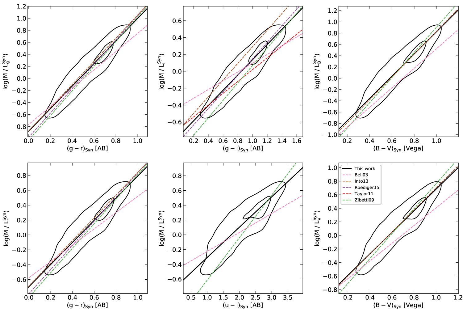
Figure 8: Comparison of the relation between restframe color and M/L for different bands for all galaxies to relations from the literature. The contours represent the density distribution encompassing 90% and 20% of the points.

6.2 Morphological MLCRs

We now turn to the effect of the SFH on the log(M/L)-color global relations. Different types of galaxies evolve in different ways, and thus, their locations in the log(M/L)-color plane are different. In principle, one would expect the relations to be different for different types of galaxies. Figure 9 compares the MLCRs at different bands for early- (red), intermediate- (green), and late-type galaxies (blue). The contours represent the density distribution encompassing 90% and 20% of the points. The dotted black line shows the best fit for all galaxy types (as in Fig. 8). The distribution of the three groups follows a sequential linear relation in the log(M/L)-color plane. Early-type galaxies are located in the high M/L and red part of the diagram, with a fairly packed and tight distribution in most filters. Intermediate galaxies spread over a larger region, centered on an intermediate region in the log(M/L)-color plane, but with a tail distribution that also encompasses similar values to those of early-type galaxies. Late-type galaxies display the widest and largest distribution of the three groups. They reach from very low values of M/L and blue colors up to relatively red colors and high M/L values.

The independent MLCRs for the three different groups are very close, in their range of validity, to the global MLCR for the whole sample. The differences between the different fits are larger when extrapolated outside the range of each distribution; thus, fits should be used only in their range of applicability. However, these differences are much smaller than the dispersion for each group distribution.

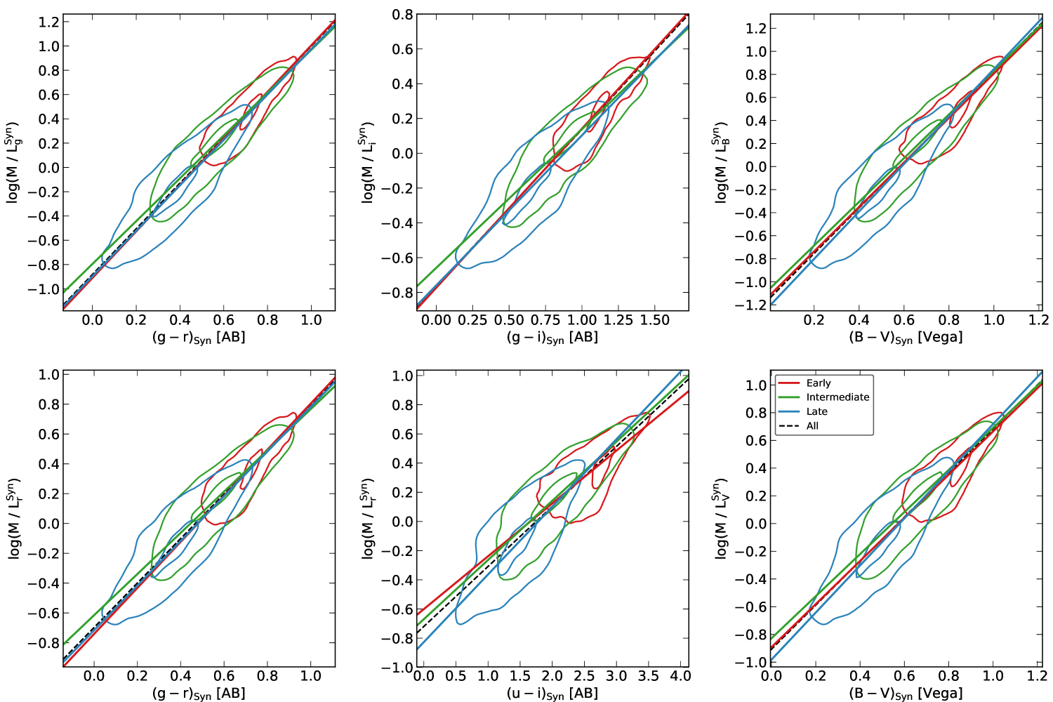
Figure 9: Relation between restframe color and M/L for different bands and for early (red), intermediate (green), and late galaxies (blue). Contours represent the density distribution encompassing 90% and 20% of the points. The dotted black line shows the best fit for all galaxy types.

6.3 Effect of the IMF

The selection of SSPs can have an effect on the M/L as well. In principle, the main contributor to this difference would be an offset due to the IMF selection, but other secondary variables can also affect the slope and/or offset of the MLCRs, such as the range of metallicities introduced in the base or the stellar evolutionary tracks used for the SSPs. To check these possible variations, we also analyzed our dataset with the base we used in García-Benito et al. (2017, hereafter GB), which assumes a Salpeter IMF. In short, it consists of a combination of 254 SSPs. It combines the granada models of González Delgado et al. (2005) for ages younger than 60 Myr and the SSPs from Vazdekis et al. (2015) based on BaSTi isochrones for older ages. The Z range covers eight metallicities, $\log Z/Z_{\odot}=-2.28$, $-1.79$, $-1.26$, $-0.66$, $-0.35$, $-0.06$, $0.25$, and $+0.40$. The age is sampled by 37 SSPs per metallicity covering from 1 Myr to 14 Gyr. The IMF is the Salpeter IMF. Dust effects were modeled in the same way as our fiducial results: as a foreground screen with a Cardelli et al. (1989) reddening law with R_V = 3.1.

Figure 10 compares the MLCRs obtained using both sets of SSPs including the whole sample in the derivations of the relations. The contours represent the density distribution encompassing 90% and 20% of the points. The wavelength range of base GB is shorter than CBe, covering from 3500 Å to 7000 Å. Thus, we only show two examples of the common filters available in both results. As expected, the distribution using GB is located higher in the log(M/L)-color plane due to the choice of a Salpeter IMF. However, in addition to the offset in the zero-points, there are some differences for very extreme colors due to the differences in the slopes. For blue colors, the relations can give M/L differences as high as 0.4 dex, while for red colors (high M/L values), this difference is on the order of 0.2 dex. Both samples have nearly the same scatter (i.e., uncertainties in the MLCRs) in the distributions.

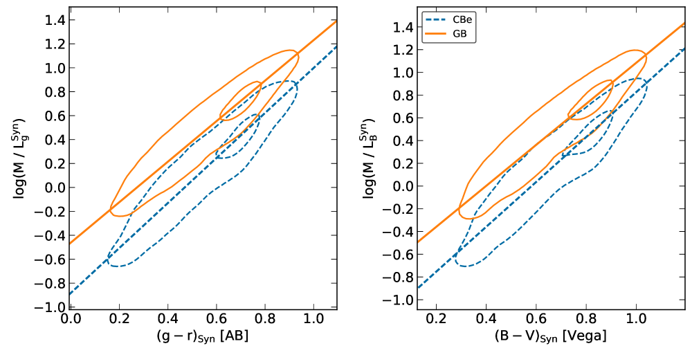
Figure 10: Comparison of the relation between restframe color and M/L for all galaxies for bases CBe (Chabrier IMF) and GB (Salpeter IMF). Contours represent the density distribution encompassing 90% and 20% of the points.

7 Summary and conclusions

We have applied the fossil record method of the stellar population to a sample of 452 galaxies observed with integral field spectroscopy in the CALIFA survey to derive the radial structure of the M/L ratio. Observed and synthetic radial colors in optical broadbands were also measured to study the spatially resolved MLCRs. Our sample covers a wide range of morphological types that includes early -type galaxies (E, S0) and spirals (Sa, Sb, Sc, Sd), and galaxy stellar masses ranges from 10^8.4 to 10¹² M_⊙. Our main results are listed below.

1. The radial profile of $M/L$ scales with Hubble type, decreasing outward in all cases. The inner gradient of M/L (within 1 HLR) is steeper than the outer gradient. The gradient is steeper in Sb-Sbc than in early types (E, S0, and Sa); late-type spirals (Sc-Sd) show the flattest gradient. These trends are independent of the photometric band used for the luminosity.

2. The spatially resolved structure of the $M/L$ ratio and colors up to 2 HLR was used to derive the MLCRs. A linear relation was derived for several pairs of $M/L$-optical colors. The mean scatter of all the combinations of filters is $\sim 0.13$ dex. A scatter lower that 0.1 dex is obtained for pairs such as ($i$, $g-r$) and ($R$, $B-R$).

3. Uncertainties associated with the effect of emission lines in the luminosity band and optical colors are very small, with the maximum difference in M/L of $\sim$ 0.02 dex, found in the r $band$ and for intermediate- and late-type galaxies, from which the largest contribution of the H$\alpha$ emission is expected in $L_{r}$. The effect of extinction is also negligible because, as pointed out by B03, the reddening correction vector runs parallel to the MLCRs at optical wavelengths.

4. The MLCRs are derived for galaxies of different Hubble types. These relations are very close, in their range of validity, to the relations found for the whole sample. The largest difference occurs for the pair ($r$, $u-i$) with an offset of 0.6 for late-type galaxies ($u-i$) ¡ 0.5 and 0.05 for early-type galaxies with ($u-i$) ¿ 3.5.

5. The effect of the SSPs used for the full spectral fitting with starlight was also studied. We compared our results in $M_{\star}$ and MLCRs derived with the bases CBe and GB. In addition to the differences in the evolutionary codes (BC03 vs. Vazdekis et al. 2015) and the corresponding stellar evolution, these two sets of SSPs have different IMFs (Chabrier vs. Salpeter). The corresponding MLCRs mainly reflect the difference in IMF, with a shift to larger $M/L$ of $\sim$ 0.29 for SSPs with Salpeter IMF. However, differences in the SFH give a random error of $\geq$ 0.4 dex for galaxies bluer than ($g-r$) = 0.2 and $\leq$ 0.2 dex for galaxies redder than ($g-r$) = 0.9.

6. The comparison of the MLCRs with other published results indicates that our relations are compatible with results based on integrated $M/L$ and color of galaxies. In particular, the relation ${\rm M/L_{B}}-(B-V)$ is very tight and perfectly agrees with them, with the exception of B03. The relations of $M/L_{g}$ and $M/L_{r}$ with ($g-r$) are remarkably similar to the relations from Zibetti et al. (2009), Into & Portinari (2013), and Roediger & Courteau (2015). However, the ${\rm M/L_{i}}-(g-i)$ plane shows greater dispersion between all the results in the literature, but our relations are similar to those of Roediger & Courteau (2015), and they are in between those of Zibetti et al. (2009) and Into & Portinari (2013) for ($g$-$i$) ¡ 1, and Taylor et al. (2011) and Into & Portinari (2013) for redder colors.

Table 1: Linear fitting at 0 $\leq$ R_HLR $\leq$ 2 to $log(M/L_{\lambda})=a_{\lambda}+(b_{\lambda}\times color)$ measured in restframe in the synthetic spectra (luminosities not corrected for reddening).

Color	$a_{u}$	$b_{u}$	$\sigma_{u}$	$a_{g}$	$b_{g}$	$\sigma_{g}$	$a_{r}$	$b_{r}$	$\sigma_{r}$	$a_{i}$	$b_{i}$	$\sigma_{i}$	$a_{z}$	$b_{z}$	$\sigma_{z}$
All galaxies
$u-g$	-1.19	1.14	0.19	-0.73	0.77	0.19	-0.57	0.60	0.16	-0.58	0.54	0.14	-0.63	0.49	0.13
$u-r$	-1.30	0.83	0.14	-0.83	0.58	0.15	-0.65	0.45	0.13	-0.65	0.40	0.12	-0.69	0.37	0.11
$u-i$	-1.40	0.74	0.12	-0.91	0.52	0.14	-0.72	0.41	0.12	-0.71	0.36	0.11	-0.74	0.33	0.11
$u-z$	-1.48	0.69	0.11	-0.97	0.48	0.13	-0.77	0.38	0.12	-0.75	0.34	0.11	-0.78	0.31	0.10
$g-r$	-1.30	2.59	0.11	-0.88	1.88	0.10	-0.70	1.49	0.10	-0.69	1.31	0.09	-0.72	1.19	0.09
$g-i$	-1.44	1.77	0.13	-0.99	1.29	0.10	-0.79	1.03	0.09	-0.77	0.90	0.09	-0.79	0.82	0.09
$g-z$	-1.52	1.43	0.15	-1.06	1.05	0.11	-0.84	0.83	0.10	-0.81	0.73	0.10	-0.83	0.66	0.10
$r-i$	-1.53	5.01	0.22	-1.08	3.74	0.15	-0.86	2.98	0.13	-0.83	2.60	0.12	-0.84	2.34	0.12
$r-z$	-1.58	2.86	0.24	-1.12	2.13	0.16	-0.89	1.70	0.14	-0.85	1.48	0.13	-0.86	1.32	0.13
$i-z$	-1.49	6.07	0.29	-1.05	4.52	0.20	-0.83	3.59	0.17	-0.80	3.11	0.16	-0.80	2.76	0.15

Table 2: Linear fitting at 0 $\leq$ R_HLR $\leq$ 2 to $log(M/L_{\lambda})=a_{\lambda}+(b_{\lambda}\times color)$ measured in restframe in the synthetic spectra (luminosities not corrected for reddening).

Color	$a_{B}$	$b_{B}$	$\sigma_{B}$	$a_{V}$	$b_{V}$	$\sigma_{V}$	$a_{R}$	$b_{R}$	$\sigma_{R}$
All galaxies
$B-V$	-1.15	1.97	0.11	-0.91	1.59	0.11	-0.82	1.36	0.10
$B-R$	-1.45	1.25	0.10	-1.15	1.01	0.10	-1.03	0.86	0.09
$V-R$	-1.83	3.22	0.12	-1.47	2.61	0.11	-1.30	2.23	0.10

Table 3: Linear fitting at 0 $\leq$ R_HLR $\leq$ 2 to $log(M/L_{\lambda})=a_{\lambda}+(b_{\lambda}\times color)$ measured in restframe in the synthetic spectra (luminosities not corrected for reddening).

Color	$a_{u}$	$b_{u}$	$\sigma_{u}$	$a_{g}$	$b_{g}$	$\sigma_{g}$	$a_{r}$	$b_{r}$	$\sigma_{r}$	$a_{i}$	$b_{i}$	$\sigma_{i}$	$a_{z}$	$b_{z}$	$\sigma_{z}$
Early galaxies
$u-g$	-0.81	0.89	0.16	-0.33	0.51	0.16	-0.25	0.40	0.14	-0.31	0.36	0.12	-0.38	0.33	0.11
$u-r$	-1.13	0.75	0.13	-0.59	0.46	0.14	-0.46	0.37	0.12	-0.49	0.33	0.11	-0.54	0.30	0.10
$u-i$	-1.32	0.71	0.11	-0.76	0.46	0.12	-0.60	0.36	0.11	-0.61	0.32	0.10	-0.64	0.29	0.09
$u-z$	-1.40	0.66	0.10	-0.85	0.44	0.12	-0.68	0.35	0.11	-0.67	0.31	0.10	-0.68	0.27	0.09
$g-r$	-1.35	2.70	0.10	-0.91	1.92	0.09	-0.74	1.55	0.09	-0.72	1.35	0.08	-0.74	1.21	0.08
$g-i$	-1.40	1.78	0.12	-0.98	1.29	0.09	-0.81	1.05	0.08	-0.77	0.92	0.08	-0.77	0.81	0.08
$g-z$	-1.38	1.37	0.13	-0.97	1.00	0.09	-0.80	0.82	0.08	-0.76	0.71	0.08	-0.76	0.62	0.08
$r-i$	-1.03	4.04	0.18	-0.79	3.14	0.12	-0.67	2.58	0.10	-0.64	2.23	0.10	-0.65	1.95	0.10
$r-z$	-1.02	2.24	0.19	-0.77	1.73	0.12	-0.65	1.42	0.11	-0.62	1.22	0.10	-0.62	1.05	0.10
$i-z$	-0.77	4.32	0.21	-0.58	3.32	0.14	-0.49	2.71	0.12	-0.48	2.30	0.11	-0.48	1.96	0.11
Intermediate galaxies
$u-g$	-1.13	1.14	0.17	-0.67	0.77	0.17	-0.51	0.59	0.15	-0.52	0.52	0.13	-0.56	0.46	0.12
$u-r$	-1.26	0.83	0.12	-0.80	0.58	0.14	-0.61	0.45	0.12	-0.60	0.39	0.11	-0.63	0.35	0.10
$u-i$	-1.35	0.73	0.11	-0.87	0.52	0.12	-0.67	0.41	0.11	-0.65	0.35	0.10	-0.68	0.31	0.10
$u-z$	-1.40	0.66	0.10	-0.92	0.48	0.11	-0.71	0.37	0.10	-0.68	0.32	0.10	-0.70	0.28	0.10
$g-r$	-1.17	2.36	0.10	-0.80	1.76	0.09	-0.62	1.38	0.09	-0.61	1.19	0.08	-0.63	1.06	0.08
$g-i$	-1.26	1.56	0.11	-0.87	1.18	0.09	-0.68	0.92	0.09	-0.66	0.80	0.09	-0.68	0.70	0.09
$g-z$	-1.30	1.22	0.13	-0.91	0.93	0.10	-0.71	0.73	0.09	-0.68	0.63	0.09	-0.69	0.55	0.09
$r-i$	-1.24	4.04	0.18	-0.88	3.13	0.13	-0.69	2.47	0.11	-0.66	2.11	0.11	-0.67	1.83	0.11
$r-z$	-1.25	2.24	0.19	-0.89	1.74	0.14	-0.69	1.37	0.12	-0.66	1.16	0.11	-0.66	1.00	0.11
$i-z$	-1.11	4.54	0.22	-0.79	3.53	0.17	-0.61	2.76	0.14	-0.58	2.33	0.13	-0.59	1.97	0.13
Late galaxies
$u-g$	-1.27	1.13	0.21	-0.84	0.81	0.21	-0.66	0.63	0.18	-0.65	0.54	0.16	-0.69	0.49	0.15
$u-r$	-1.38	0.86	0.16	-0.96	0.65	0.17	-0.76	0.51	0.15	-0.74	0.44	0.14	-0.77	0.40	0.13
$u-i$	-1.46	0.76	0.14	-1.04	0.59	0.15	-0.83	0.46	0.14	-0.80	0.40	0.13	-0.81	0.36	0.13
$u-z$	-1.52	0.70	0.13	-1.09	0.54	0.15	-0.87	0.43	0.14	-0.83	0.37	0.13	-0.84	0.33	0.12
$g-r$	-1.21	2.31	0.12	-0.90	1.87	0.12	-0.72	1.50	0.11	-0.70	1.30	0.11	-0.73	1.16	0.11
$g-i$	-1.31	1.52	0.13	-0.98	1.25	0.12	-0.79	1.00	0.11	-0.76	0.86	0.11	-0.78	0.77	0.11
$g-z$	-1.37	1.20	0.14	-1.03	0.99	0.13	-0.83	0.79	0.12	-0.79	0.68	0.11	-0.81	0.60	0.11
$r-i$	-1.32	3.82	0.20	-1.01	3.20	0.16	-0.81	2.57	0.14	-0.78	2.20	0.13	-0.79	1.95	0.13
$r-z$	-1.37	2.16	0.21	-1.04	1.79	0.17	-0.83	1.44	0.15	-0.79	1.23	0.14	-0.80	1.08	0.14
$i-z$	-1.27	4.30	0.24	-0.96	3.54	0.20	-0.76	2.83	0.17	-0.73	2.39	0.16	-0.74	2.07	0.15

Table 4: Linear fitting at 0 $\leq$ R_HLR $\leq$ 2 to $log(M/L_{\lambda})=a_{\lambda}+(b_{\lambda}\times color)$ measured in restframe in the synthetic spectra (luminosities not corrected for reddening).

Color	$a_{B}$	$b_{B}$	$\sigma_{B}$	$a_{V}$	$b_{V}$	$\sigma_{V}$	$a_{R}$	$b_{R}$	$\sigma_{R}$
Early galaxies
$B-V$	-1.12	1.93	0.10	-0.89	1.56	0.10	-0.81	1.33	0.09
$B-R$	-1.46	1.26	0.09	-1.19	1.03	0.08	-1.06	0.88	0.08
$V-R$	-1.62	2.96	0.11	-1.34	2.46	0.09	-1.19	2.10	0.09
Intermediate galaxies
$B-V$	-1.06	1.90	0.10	-0.83	1.52	0.10	-0.74	1.28	0.09
$B-R$	-1.32	1.17	0.09	-1.03	0.94	0.09	-0.91	0.79	0.08
$V-R$	-1.57	2.81	0.11	-1.25	2.27	0.10	-1.09	1.90	0.10
Late galaxies
$B-V$	-1.21	2.06	0.13	-0.98	1.70	0.13	-0.88	1.43	0.12
$B-R$	-1.47	1.26	0.12	-1.20	1.04	0.12	-1.06	0.88	0.11
$V-R$	-1.71	2.92	0.13	-1.41	2.43	0.12	-1.23	2.05	0.12

Table 5: Linear fitting at 0 $\leq$ R_HLR $\leq$ 2 to $log(M/L_{\lambda})=a_{\lambda}+(b_{\lambda}\times color)$ measured in restframe in the synthetic spectra (luminosities not corrected for reddening).

Color	$a_{B}$	$b_{B}$	$\sigma_{B}$	$a_{V}$	$b_{V}$	$\sigma_{V}$	$a_{R}$	$b_{R}$	$\sigma_{R}$
E galaxies
$B-V$	-1.81	2.69	0.09	-1.57	2.30	0.08	-1.44	2.03	0.08
$B-R$	-2.05	1.62	0.07	-1.78	1.40	0.07	-1.63	1.23	0.07
$V-R$	-2.12	3.69	0.08	-1.85	3.18	0.07	-1.68	2.80	0.07
S0 galaxies
$B-V$	-1.25	2.07	0.10	-1.03	1.70	0.10	-0.94	1.47	0.09
$B-R$	-1.58	1.33	0.08	-1.32	1.11	0.08	-1.19	0.96	0.08
$V-R$	-1.81	3.25	0.09	-1.53	2.73	0.08	-1.38	2.38	0.08
Sa galaxies
$B-V$	-0.92	1.73	0.09	-0.70	1.36	0.09	-0.63	1.15	0.08
$B-R$	-1.20	1.11	0.09	-0.93	0.88	0.08	-0.82	0.73	0.08
$V-R$	-1.28	2.47	0.12	-1.00	1.98	0.10	-0.86	1.63	0.10
Sb galaxies
$B-V$	-1.02	1.84	0.10	-0.78	1.46	0.10	-0.69	1.21	0.09
$B-R$	-1.26	1.13	0.09	-0.98	0.90	0.09	-0.85	0.75	0.08
$V-R$	-1.47	2.68	0.11	-1.15	2.15	0.10	-0.99	1.78	0.09
Sbc galaxies
$B-V$	-1.09	1.93	0.10	-0.86	1.56	0.09	-0.77	1.32	0.09
$B-R$	-1.34	1.18	0.09	-1.06	0.96	0.09	-0.94	0.81	0.08
$V-R$	-1.58	2.80	0.11	-1.27	2.29	0.10	-1.11	1.92	0.09
Sc galaxies
$B-V$	-1.15	1.98	0.13	-0.92	1.61	0.13	-0.82	1.36	0.12
$B-R$	-1.42	1.22	0.12	-1.15	1.00	0.12	-1.02	0.84	0.11
$V-R$	-1.63	2.79	0.14	-1.33	2.31	0.12	-1.17	1.94	0.12
Sd galaxies
$B-V$	-1.18	1.91	0.12	-0.96	1.58	0.12	-0.86	1.32	0.11
$B-R$	-1.47	1.23	0.11	-1.20	1.02	0.11	-1.06	0.86	0.10
$V-R$	-1.72	2.90	0.12	-1.42	2.42	0.11	-1.24	2.03	0.11

Appendix A Intrinsic mass-to-light color relations

In this appendix we include the intrinsic mass-to-light color relations, that is, the MLRC where the luminosities have been corrected for reddening. These relations can be useful for comparison with models or simulations.

Table 6: Linear fitting at 0 $\leq$ R_HLR $\leq$ 2 to $log(M/L_{\lambda})=a_{\lambda}+(b_{\lambda}\times color)$ measured in restframe in the synthetic spectra and corrected for reddening (i.e. intrinsic luminosities).

Color	$a_{u}$	$b_{u}$	$\sigma_{u}$	$a_{g}$	$b_{g}$	$\sigma_{g}$	$a_{r}$	$b_{r}$	$\sigma_{r}$	$a_{i}$	$b_{i}$	$\sigma_{i}$	$a_{z}$	$b_{z}$	$\sigma_{z}$
All galaxies
$u-g$	-1.26	1.15	0.18	-0.78	0.77	0.18	-0.59	0.60	0.16	-0.59	0.52	0.14	-0.61	0.47	0.13
$u-r$	-1.29	0.82	0.14	-0.82	0.56	0.15	-0.63	0.43	0.14	-0.62	0.38	0.12	-0.64	0.34	0.12
$u-i$	-1.36	0.73	0.12	-0.87	0.50	0.14	-0.67	0.39	0.13	-0.66	0.34	0.12	-0.68	0.31	0.11
$u-z$	-1.41	0.67	0.12	-0.91	0.46	0.13	-0.70	0.36	0.12	-0.68	0.32	0.11	-0.70	0.29	0.11
$g-r$	-1.25	2.58	0.10	-0.82	1.82	0.11	-0.63	1.43	0.10	-0.63	1.26	0.09	-0.65	1.14	0.09
$g-i$	-1.40	1.80	0.09	-0.93	1.28	0.09	-0.72	1.01	0.09	-0.70	0.89	0.09	-0.73	0.80	0.09
$g-z$	-1.48	1.47	0.10	-0.99	1.05	0.10	-0.77	0.82	0.09	-0.75	0.72	0.09	-0.76	0.66	0.09
$r-i$	-1.63	5.62	0.15	-1.11	4.02	0.11	-0.87	3.18	0.10	-0.83	2.80	0.09	-0.84	2.53	0.09
$r-z$	-1.69	3.24	0.16	-1.14	2.31	0.12	-0.89	1.82	0.11	-0.85	1.60	0.10	-0.86	1.44	0.10
$i-z$	-1.66	7.23	0.20	-1.11	5.11	0.16	-0.87	4.03	0.13	-0.83	3.53	0.12	-0.83	3.17	0.12

Table 7: Linear fitting at 0 $\leq$ R_HLR $\leq$ 2 to $log(M/L_{\lambda})=a_{\lambda}+(b_{\lambda}\times color)$ measured in restframe in the synthetic spectra and corrected for reddening (i.e. intrinsic luminosities).

Color	$a_{B}$	$b_{B}$	$\sigma_{B}$	$a_{V}$	$b_{V}$	$\sigma_{V}$	$a_{R}$	$b_{R}$	$\sigma_{R}$
All galaxies
$B-V$	-1.08	1.89	0.12	-0.83	1.50	0.11	-0.75	1.28	0.11
$B-R$	-1.38	1.23	0.10	-1.07	0.98	0.10	-0.95	0.83	0.09
$V-R$	-1.85	3.34	0.10	-1.45	2.67	0.09	-1.28	2.28	0.09

Table 8: Linear fitting at 0 $\leq$ R_HLR $\leq$ 2 to $log(M/L_{\lambda})=a_{\lambda}+(b_{\lambda}\times color)$ measured in restframe in the synthetic spectra and corrected for reddening (i.e. intrinsic luminosities).

Color	$a_{u}$	$b_{u}$	$\sigma_{u}$	$a_{g}$	$b_{g}$	$\sigma_{g}$	$a_{r}$	$b_{r}$	$\sigma_{r}$	$a_{i}$	$b_{i}$	$\sigma_{i}$	$a_{z}$	$b_{z}$	$\sigma_{z}$
Early galaxies
$u-g$	-0.94	0.95	0.14	-0.44	0.56	0.14	-0.30	0.42	0.12	-0.33	0.36	0.11	-0.38	0.32	0.11
$u-r$	-1.09	0.73	0.12	-0.56	0.44	0.12	-0.40	0.33	0.11	-0.42	0.29	0.11	-0.46	0.26	0.10
$u-i$	-1.22	0.67	0.11	-0.65	0.41	0.12	-0.48	0.31	0.11	-0.49	0.27	0.10	-0.52	0.24	0.10
$u-z$	-1.28	0.62	0.10	-0.70	0.39	0.11	-0.52	0.30	0.11	-0.52	0.26	0.10	-0.55	0.23	0.10
$g-r$	-1.32	2.68	0.09	-0.77	1.74	0.10	-0.59	1.35	0.09	-0.59	1.19	0.09	-0.62	1.07	0.08
$g-i$	-1.50	1.90	0.08	-0.92	1.25	0.08	-0.71	0.99	0.08	-0.69	0.87	0.08	-0.71	0.78	0.08
$g-z$	-1.54	1.52	0.08	-0.96	1.01	0.08	-0.75	0.80	0.08	-0.72	0.70	0.08	-0.73	0.63	0.08
$r-i$	-1.51	5.36	0.13	-1.00	3.73	0.09	-0.80	3.01	0.08	-0.77	2.64	0.08	-0.78	2.36	0.08
$r-z$	-1.50	3.00	0.14	-0.98	2.07	0.10	-0.78	1.66	0.09	-0.75	1.45	0.09	-0.75	1.29	0.09
$i-z$	-1.31	6.19	0.17	-0.82	4.17	0.13	-0.65	3.32	0.11	-0.63	2.89	0.10	-0.63	2.53	0.10
Intermediate galaxies
$u-g$	-1.15	1.09	0.17	-0.67	0.71	0.16	-0.49	0.55	0.14	-0.50	0.48	0.13	-0.53	0.43	0.12
$u-r$	-1.23	0.80	0.13	-0.75	0.54	0.14	-0.56	0.42	0.12	-0.56	0.37	0.11	-0.59	0.33	0.11
$u-i$	-1.31	0.72	0.11	-0.82	0.49	0.13	-0.62	0.38	0.11	-0.61	0.34	0.11	-0.64	0.30	0.10
$u-z$	-1.37	0.66	0.11	-0.86	0.46	0.12	-0.66	0.36	0.11	-0.64	0.31	0.10	-0.67	0.28	0.10
$g-r$	-1.20	2.51	0.09	-0.79	1.80	0.10	-0.60	1.42	0.09	-0.60	1.25	0.08	-0.63	1.14	0.08
$g-i$	-1.36	1.75	0.09	-0.90	1.27	0.09	-0.70	1.00	0.08	-0.68	0.88	0.08	-0.70	0.80	0.08
$g-z$	-1.45	1.44	0.09	-0.97	1.04	0.09	-0.75	0.82	0.08	-0.73	0.73	0.08	-0.75	0.66	0.08
$r-i$	-1.54	5.28	0.13	-1.06	3.89	0.10	-0.83	3.09	0.09	-0.79	2.73	0.08	-0.81	2.47	0.08
$r-z$	-1.61	3.07	0.14	-1.10	2.25	0.11	-0.86	1.79	0.09	-0.82	1.58	0.09	-0.83	1.43	0.09
$i-z$	-1.52	6.58	0.18	-1.03	4.80	0.14	-0.81	3.81	0.12	-0.77	3.35	0.11	-0.78	3.01	0.11
Late galaxies
$u-g$	-1.25	1.02	0.20	-0.81	0.69	0.20	-0.62	0.53	0.18	-0.62	0.47	0.16	-0.65	0.43	0.15
$u-r$	-1.34	0.82	0.16	-0.91	0.58	0.17	-0.71	0.46	0.16	-0.69	0.41	0.14	-0.72	0.38	0.14
$u-i$	-1.43	0.75	0.14	-0.99	0.55	0.16	-0.77	0.44	0.15	-0.75	0.39	0.13	-0.78	0.36	0.13
$u-z$	-1.50	0.71	0.14	-1.04	0.52	0.15	-0.82	0.41	0.14	-0.79	0.37	0.13	-0.81	0.34	0.13
$g-r$	-1.22	2.44	0.12	-0.87	1.91	0.13	-0.68	1.54	0.12	-0.67	1.37	0.11	-0.71	1.27	0.11
$g-i$	-1.36	1.73	0.12	-0.99	1.37	0.12	-0.79	1.11	0.11	-0.77	0.99	0.10	-0.79	0.91	0.10
$g-z$	-1.45	1.43	0.12	-1.07	1.13	0.12	-0.85	0.92	0.11	-0.82	0.81	0.11	-0.83	0.75	0.10
$r-i$	-1.46	4.70	0.18	-1.10	3.85	0.15	-0.88	3.14	0.13	-0.84	2.77	0.12	-0.86	2.55	0.12
$r-z$	-1.53	2.78	0.19	-1.15	2.24	0.15	-0.92	1.82	0.13	-0.87	1.60	0.13	-0.88	1.46	0.12
$i-z$	-1.39	5.33	0.23	-1.01	4.17	0.19	-0.80	3.36	0.16	-0.76	2.93	0.15	-0.78	2.65	0.15

Table 9: Linear fitting at 0 $\leq$ R_HLR $\leq$ 2 to $log(M/L_{\lambda})=a_{\lambda}+(b_{\lambda}\times color)$ measured in restframe in the synthetic spectra and corrected for reddening (i.e. intrinsic luminosities).

Color	$a_{B}$	$b_{B}$	$\sigma_{B}$	$a_{V}$	$b_{V}$	$\sigma_{V}$	$a_{R}$	$b_{R}$	$\sigma_{R}$
Early galaxies
$B-V$	-0.95	1.72	0.10	-0.70	1.33	0.10	-0.64	1.13	0.10
$B-R$	-1.31	1.17	0.09	-1.00	0.92	0.09	-0.89	0.78	0.09
$V-R$	-1.84	3.33	0.08	-1.45	2.66	0.08	-1.28	2.28	0.08
Intermediate galaxies
$B-V$	-1.03	1.87	0.11	-0.79	1.48	0.10	-0.71	1.26	0.09
$B-R$	-1.34	1.22	0.09	-1.04	0.97	0.09	-0.92	0.83	0.08
$V-R$	-1.81	3.29	0.09	-1.42	2.64	0.09	-1.25	2.26	0.08
Late galaxies
$B-V$	-1.18	2.05	0.14	-0.94	1.69	0.13	-0.85	1.45	0.12
$B-R$	-1.50	1.34	0.12	-1.21	1.11	0.12	-1.08	0.96	0.11
$V-R$	-1.85	3.31	0.13	-1.51	2.76	0.12	-1.34	2.38	0.11

5]

Table 10: Linear fitting at 0 $\leq$ R_HLR $\leq$ 2 to $log(M/L_{\lambda})=a_{\lambda}+(b_{\lambda}\times color)$ measured in restframe in the synthetic spectra and corrected for reddening (i.e. intrinsic luminosities).

Color	$a_{u}$	$b_{u}$	$\sigma_{u}$	$a_{g}$	$b_{g}$	$\sigma_{g}$	$a_{r}$	$b_{r}$	$\sigma_{r}$	$a_{i}$	$b_{i}$	$\sigma_{i}$	$a_{z}$	$b_{z}$	$\sigma_{z}$
E galaxies
$u-g$	-1.54	1.30	0.13	-1.01	0.89	0.13	-0.85	0.73	0.12	-0.81	0.64	0.11	-0.80	0.56	0.11
$u-r$	-1.78	1.00	0.11	-1.24	0.71	0.11	-1.06	0.60	0.11	-1.00	0.53	0.10	-0.98	0.47	0.10
$u-i$	-1.84	0.88	0.10	-1.31	0.64	0.10	-1.13	0.54	0.10	-1.07	0.48	0.09	-1.05	0.43	0.09
$u-z$	-1.82	0.79	0.09	-1.31	0.58	0.10	-1.13	0.49	0.10	-1.07	0.43	0.09	-1.05	0.39	0.09
$g-r$	-1.85	3.41	0.08	-1.44	2.63	0.08	-1.26	2.24	0.08	-1.20	2.01	0.08	-1.19	1.83	0.08
$g-i$	-1.77	2.14	0.06	-1.39	1.66	0.07	-1.23	1.43	0.07	-1.17	1.27	0.07	-1.16	1.16	0.07
$g-z$	-1.73	1.65	0.07	-1.35	1.27	0.07	-1.18	1.09	0.07	-1.13	0.97	0.07	-1.12	0.88	0.07
$r-i$	-1.44	5.24	0.08	-1.13	4.05	0.07	-1.00	3.48	0.07	-0.97	3.11	0.07	-0.97	2.82	0.07
$r-z$	-1.43	2.92	0.09	-1.11	2.24	0.08	-0.98	1.93	0.08	-0.95	1.71	0.08	-0.95	1.55	0.08
$i-z$	-1.23	5.99	0.12	-0.92	4.50	0.11	-0.81	3.83	0.10	-0.79	3.38	0.09	-0.79	3.02	0.09
S0 galaxies
$u-g$	-1.04	1.01	0.14	-0.55	0.62	0.13	-0.41	0.47	0.12	-0.42	0.41	0.11	-0.45	0.36	0.11
$u-r$	-1.22	0.78	0.12	-0.70	0.50	0.12	-0.54	0.39	0.11	-0.54	0.34	0.10	-0.56	0.30	0.10
$u-i$	-1.33	0.71	0.10	-0.80	0.46	0.11	-0.63	0.36	0.11	-0.61	0.32	0.10	-0.63	0.28	0.10
$u-z$	-1.38	0.65	0.10	-0.85	0.43	0.11	-0.67	0.34	0.10	-0.65	0.30	0.10	-0.66	0.26	0.09
$g-r$	-1.36	2.74	0.09	-0.91	1.91	0.09	-0.73	1.54	0.09	-0.71	1.35	0.08	-0.72	1.21	0.08
$g-i$	-1.52	1.91	0.07	-1.01	1.33	0.08	-0.83	1.08	0.08	-0.80	0.96	0.07	-0.81	0.86	0.07
$g-z$	-1.58	1.54	0.07	-1.04	1.07	0.08	-0.85	0.86	0.08	-0.82	0.76	0.07	-0.82	0.68	0.07
$r-i$	-1.49	5.33	0.10	-1.06	3.88	0.08	-0.88	3.18	0.07	-0.84	2.81	0.07	-0.85	2.53	0.07
$r-z$	-1.50	3.01	0.11	-1.06	2.18	0.09	-0.87	1.78	0.08	-0.84	1.57	0.08	-0.83	1.40	0.08
$i-z$	-1.33	6.30	0.14	-0.91	4.49	0.11	-0.75	3.65	0.10	-0.72	3.19	0.09	-0.72	2.83	0.09
Sa galaxies
$u-g$	-0.90	0.94	0.14	-0.40	0.55	0.14	-0.27	0.41	0.12	-0.30	0.36	0.11	-0.35	0.32	0.10
$u-r$	-1.04	0.72	0.12	-0.51	0.43	0.12	-0.35	0.32	0.11	-0.38	0.29	0.10	-0.43	0.26	0.09
$u-i$	-1.16	0.66	0.11	-0.59	0.40	0.11	-0.42	0.30	0.10	-0.44	0.27	0.09	-0.48	0.24	0.09
$u-z$	-1.23	0.61	0.10	-0.64	0.38	0.11	-0.46	0.29	0.10	-0.47	0.25	0.09	-0.51	0.22	0.09
$g-r$	-1.21	2.52	0.10	-0.68	1.63	0.09	-0.49	1.24	0.09	-0.51	1.11	0.08	-0.55	1.01	0.08
$g-i$	-1.40	1.81	0.09	-0.83	1.19	0.08	-0.62	0.92	0.08	-0.62	0.81	0.07	-0.64	0.73	0.07
$g-z$	-1.47	1.46	0.10	-0.89	0.97	0.08	-0.67	0.76	0.08	-0.65	0.66	0.08	-0.67	0.59	0.08
$r-i$	-1.46	5.14	0.17	-0.91	3.50	0.11	-0.70	2.77	0.09	-0.68	2.42	0.09	-0.69	2.16	0.09
$r-z$	-1.45	2.88	0.18	-0.89	1.95	0.12	-0.69	1.53	0.10	-0.67	1.34	0.10	-0.67	1.18	0.10
$i-z$	-1.23	5.77	0.21	-0.72	3.80	0.15	-0.54	2.96	0.12	-0.53	2.57	0.11	-0.54	2.24	0.11
Sb galaxies
$u-g$	-1.04	1.02	0.16	-0.57	0.65	0.16	-0.41	0.49	0.14	-0.42	0.42	0.12	-0.46	0.38	0.12
$u-r$	-1.15	0.76	0.13	-0.66	0.49	0.13	-0.48	0.38	0.12	-0.48	0.33	0.11	-0.52	0.30	0.11
$u-i$	-1.24	0.68	0.11	-0.73	0.45	0.12	-0.54	0.34	0.11	-0.53	0.30	0.10	-0.57	0.27	0.10
$u-z$	-1.30	0.64	0.11	-0.78	0.42	0.12	-0.57	0.32	0.11	-0.57	0.28	0.10	-0.59	0.25	0.10
$g-r$	-1.19	2.49	0.10	-0.74	1.73	0.10	-0.56	1.34	0.09	-0.55	1.17	0.09	-0.59	1.06	0.08
$g-i$	-1.34	1.74	0.09	-0.86	1.22	0.09	-0.65	0.95	0.09	-0.64	0.83	0.08	-0.66	0.75	0.08
$g-z$	-1.44	1.44	0.09	-0.93	1.01	0.09	-0.71	0.78	0.08	-0.69	0.69	0.08	-0.70	0.62	0.08
$r-i$	-1.52	5.26	0.12	-1.01	3.76	0.10	-0.78	2.95	0.09	-0.75	2.59	0.08	-0.76	2.33	0.08
$r-z$	-1.60	3.08	0.12	-1.06	2.18	0.10	-0.82	1.71	0.09	-0.78	1.50	0.08	-0.79	1.35	0.08
$i-z$	-1.51	6.60	0.17	-0.99	4.65	0.13	-0.76	3.65	0.11	-0.73	3.19	0.10	-0.73	2.85	0.10
Sbc galaxies
$u-g$	-1.19	1.11	0.17	-0.72	0.74	0.17	-0.54	0.58	0.15	-0.54	0.51	0.13	-0.58	0.47	0.13
$u-r$	-1.28	0.83	0.13	-0.82	0.58	0.14	-0.62	0.46	0.12	-0.62	0.40	0.11	-0.65	0.37	0.11
$u-i$	-1.37	0.74	0.11	-0.89	0.53	0.13	-0.69	0.42	0.11	-0.68	0.37	0.11	-0.70	0.34	0.10
$u-z$	-1.43	0.69	0.10	-0.94	0.50	0.12	-0.73	0.39	0.11	-0.71	0.35	0.10	-0.74	0.32	0.10
$g-r$	-1.20	2.48	0.08	-0.82	1.88	0.09	-0.64	1.50	0.08	-0.64	1.33	0.08	-0.67	1.23	0.08
$g-i$	-1.35	1.74	0.08	-0.94	1.32	0.08	-0.74	1.06	0.08	-0.72	0.94	0.07	-0.75	0.87	0.07
$g-z$	-1.44	1.43	0.09	-1.02	1.09	0.08	-0.80	0.87	0.08	-0.77	0.78	0.07	-0.79	0.71	0.07
$r-i$	-1.51	5.10	0.13	-1.09	3.99	0.11	-0.86	3.22	0.09	-0.83	2.86	0.09	-0.85	2.62	0.08
$r-z$	-1.57	2.97	0.15	-1.14	2.32	0.12	-0.90	1.87	0.10	-0.87	1.66	0.09	-0.88	1.52	0.09
$i-z$	-1.45	6.14	0.19	-1.04	4.77	0.15	-0.82	3.87	0.13	-0.79	3.42	0.12	-0.80	3.10	0.11
Sc galaxies
$u-g$	-1.13	0.93	0.19	-0.68	0.59	0.19	-0.51	0.45	0.17	-0.52	0.40	0.15	-0.57	0.37	0.15
$u-r$	-1.26	0.77	0.15	-0.81	0.53	0.16	-0.62	0.41	0.15	-0.62	0.37	0.14	-0.66	0.35	0.13
$u-i$	-1.37	0.72	0.13	-0.91	0.51	0.15	-0.70	0.40	0.14	-0.70	0.36	0.13	-0.73	0.34	0.13
$u-z$	-1.44	0.68	0.13	-0.97	0.49	0.15	-0.75	0.39	0.14	-0.74	0.35	0.13	-0.76	0.32	0.12
$g-r$	-1.19	2.39	0.12	-0.83	1.83	0.12	-0.65	1.47	0.12	-0.65	1.32	0.11	-0.68	1.23	0.11
$g-i$	-1.35	1.72	0.11	-0.97	1.35	0.11	-0.77	1.09	0.11	-0.75	0.98	0.10	-0.78	0.91	0.10
$g-z$	-1.44	1.42	0.12	-1.05	1.12	0.11	-0.83	0.91	0.11	-0.81	0.81	0.10	-0.83	0.75	0.10
$r-i$	-1.40	4.53	0.18	-1.06	3.73	0.14	-0.85	3.06	0.13	-0.82	2.72	0.12	-0.84	2.50	0.12
$r-z$	-1.46	2.66	0.18	-1.09	2.15	0.15	-0.88	1.76	0.13	-0.84	1.56	0.12	-0.85	1.43	0.12
$i-z$	-1.25	4.76	0.22	-0.88	3.70	0.18	-0.70	3.00	0.15	-0.68	2.63	0.14	-0.70	2.39	0.14
Sd galaxies
$u-g$	-1.23	0.83	0.19	-0.79	0.49	0.19	-0.61	0.36	0.16	-0.60	0.31	0.15	-0.63	0.28	0.14
$u-r$	-1.31	0.70	0.16	-0.87	0.45	0.16	-0.67	0.34	0.15	-0.66	0.30	0.13	-0.69	0.27	0.13
$u-i$	-1.39	0.66	0.14	-0.94	0.44	0.15	-0.72	0.34	0.14	-0.70	0.29	0.13	-0.73	0.26	0.12
$u-z$	-1.45	0.63	0.14	-0.98	0.42	0.15	-0.76	0.32	0.14	-0.73	0.28	0.13	-0.75	0.25	0.12
$g-r$	-1.21	2.31	0.13	-0.86	1.74	0.12	-0.67	1.36	0.12	-0.66	1.20	0.11	-0.69	1.10	0.10
$g-i$	-1.33	1.62	0.13	-0.97	1.25	0.12	-0.76	0.98	0.11	-0.73	0.85	0.10	-0.75	0.78	0.10
$g-z$	-1.41	1.33	0.13	-1.02	1.01	0.12	-0.80	0.79	0.11	-0.77	0.68	0.11	-0.78	0.62	0.10
$r-i$	-1.40	4.11	0.18	-1.03	3.22	0.14	-0.81	2.55	0.13	-0.77	2.19	0.12	-0.79	1.98	0.11
$r-z$	-1.46	2.38	0.19	-1.05	1.82	0.15	-0.83	1.42	0.13	-0.78	1.22	0.12	-0.80	1.09	0.12
$i-z$	-1.32	4.19	0.22	-0.92	3.05	0.18	-0.72	2.36	0.15	-0.69	2.00	0.14	-0.71	1.75	0.13

Table 10: continued.

Table 11: Linear fitting at 0 $\leq$ R_HLR $\leq$ 2 to $log(M/L_{\lambda})=a_{\lambda}+(b_{\lambda}\times color)$ measured in restframe in the synthetic spectra and corrected for reddening (i.e. intrinsic luminosities).

Color	$a_{B}$	$b_{B}$	$\sigma_{B}$	$a_{V}$	$b_{V}$	$\sigma_{V}$	$a_{R}$	$b_{R}$	$\sigma_{R}$
E galaxies
$B-V$	-1.73	2.60	0.09	-1.50	2.23	0.09	-1.38	1.97	0.09
$B-R$	-2.03	1.62	0.08	-1.77	1.40	0.08	-1.63	1.24	0.08
$V-R$	-2.29	3.95	0.07	-2.01	3.42	0.07	-1.84	3.04	0.07
S0 galaxies
$B-V$	-1.11	1.90	0.10	-0.87	1.51	0.10	-0.79	1.30	0.09
$B-R$	-1.45	1.26	0.09	-1.17	1.02	0.09	-1.05	0.88	0.08
$V-R$	-1.93	3.45	0.07	-1.56	2.81	0.07	-1.40	2.44	0.07
Sa galaxies
$B-V$	-0.86	1.64	0.10	-0.61	1.25	0.09	-0.56	1.07	0.09
$B-R$	-1.21	1.12	0.09	-0.90	0.87	0.08	-0.80	0.74	0.08
$V-R$	-1.71	3.15	0.09	-1.30	2.47	0.08	-1.15	2.11	0.08
Sb galaxies
$B-V$	-0.96	1.77	0.11	-0.71	1.37	0.10	-0.64	1.16	0.10
$B-R$	-1.27	1.16	0.10	-0.96	0.91	0.09	-0.85	0.77	0.09
$V-R$	-1.73	3.17	0.10	-1.33	2.51	0.09	-1.17	2.13	0.08
Sbc galaxies
$B-V$	-1.08	1.95	0.10	-0.84	1.57	0.10	-0.76	1.36	0.09
$B-R$	-1.41	1.27	0.09	-1.11	1.03	0.08	-0.99	0.89	0.08
$V-R$	-1.86	3.40	0.09	-1.49	2.77	0.08	-1.32	2.39	0.08
Sc galaxies
$B-V$	-1.10	1.91	0.13	-0.86	1.56	0.13	-0.78	1.35	0.12
$B-R$	-1.44	1.29	0.12	-1.15	1.06	0.11	-1.04	0.92	0.11
$V-R$	-1.81	3.26	0.12	-1.47	2.71	0.12	-1.31	2.35	0.11
Sd galaxies
$B-V$	-1.17	1.91	0.13	-0.93	1.55	0.13	-0.83	1.31	0.12
$B-R$	-1.45	1.24	0.12	-1.16	1.01	0.12	-1.03	0.86	0.11
$V-R$	-1.72	2.95	0.13	-1.39	2.41	0.12	-1.21	2.03	0.11