A Baseline for Multi-Label Image Classification Using An Ensemble of Deep Convolutional Neural Networks

Abstract

Recent studies on multi-label image classification have focused on designing more complex architectures of deep neural networks such as the use of attention mechanisms and region proposal networks. Although performance gains have been reported, the backbone deep models of the proposed approaches and the evaluation metrics employed in different works vary, making it difficult to compare fairly. Moreover, due to the lack of properly investigated baselines, the advantage introduced by the proposed techniques are often ambiguous. To address these issues, we make a thorough investigation of the mainstream deep convolutional neural network architectures for multi-label image classification and present a strong baseline. With the use of proper data augmentation techniques and model ensembles, the basic deep architectures can achieve better performance than many existing more complex ones on three benchmark datasets, providing great insight for the future studies on multi-label image classification.

Index Terms—  Multi-Label Image Classification, Deep Convolutional Neural Network, Data Augmentation

1 Introduction

Multi-label image classification has been a hot topic in computer vision community. Its extensive applications include but are not limited to image retrieval, automatic image annotation, web image search and image tagging [1, 2, 3, 4, 5].

The abundant labelled data (e.g. ImageNet [6]) and advanced computational hardware have promoted the development of deep convolutional neural network (CNN) based methods on single-label image classification [7, 8]. Recently, such successful models have been extended to multi-label classification tasks with promising performance reported by [9, 10, 11, 12, 13, 14, 15], proving that CNN models are capable of handling this challenging and more general problem. However, due to the varying backbones [15, 16] employed in the deep models, the achieved performance cannot be directly compared with each other. In addition, the lack of thoroughly investigated baselines of these deep CNN models hinders an explicit evaluation of the benefit brought by advanced frameworks specially designed for multi-label image classification.

To address the aforementioned issues, we present a thorough investigation on different baseline deep CNN models for multi-label image classification. We focus on two state-of-the-art deep CNN architectures (i.e., VGG16 [17] and ResNet101[8]) as they have been widely employed in multi-label image classification [12, 15]. We evaluate the models by taking advantage of varying data augmentation techniques and model ensemble, surprisingly achieving comparable or superior performance on three benchmark datasets than the state-of-the-art results achieved by more complex models.

The contributions of this work are summarized as follows:

• We investigate the impacts of varying image sizes and data augmentation techniques including “mixup” which has not been employed in multi-label image classification.

• We use score level fusion to investigate the complementarity of different models and point out possible directions for future model design.

• We present a strong baseline for multi-label image classification with performance comparable with state-of-the-art on three benchmark datasets.

2 Related Work

Impressive progress on multi-label image classification has been made by using deep convolutional neural networks. Wang et al. [9] propose a CNN-RNN framework to explore label co-occurrence using the long-short term memory (LSTM). Although VGG16 was employed as a visual feature extractor, the model capacity was not fully exploited by fine-tuning the parameters. Zhang et al. [15] extend the idea by improving the component CNN. They propose a regional latent semantic dependencies (RLSD) model for multi-label image classification, which focuses on small objects in multi-label images by generating subregions that potentially contain multiple objects and visual concepts. An LSTM based model is employed to generate multiple labels. Recently, attention mechanisms have been introduced to deep neural networks for multi-label image classification. It aims to explicitly or implicitly extract multiple visual representations from a single image characterizing different associated labels [10, 12]. The advantage of combining multi-scale input images for multi-label image classification has been proved in [18, 19] by employing varying fusion approaches.

Although improved performance has been reported by introducing more advanced frameworks, we notice that the performance of those proposed methods has marginal gains towards the standard (“vanilla”) deep models, and the training techniques employed in different works vary. Therefore it is necessary to set up a uniform baseline for comparison.

3 Method

We present the methods used to produce the strong baseline performance in this section. We first formulate the multi-label image classification problem. Subsequently, we describe the adapted deep convolutional neural networks for multi-label classification, as well as the essential data augmentation techniques for training an improved deep model. Finally, A simple yet effective model ensemble approach is introduced to investigate the complementarity of different models.

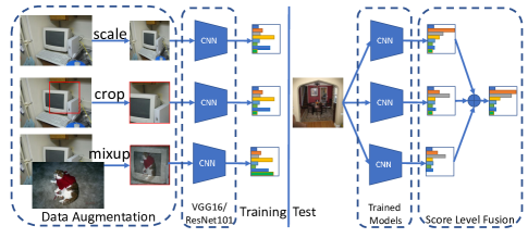
Fig. 1: An illustration of the employed framework. Varying image scales and data augmentation techniques are used during training which results in diverse trained models. These models are used for testing individually and combined by score level fusion.

3.1 Problem Formulation

Assume we have a set of training examples $\mathcal{D}=\{(\bm{x}_{i},\bm{y}_{i})\},i=1,2,...,n$, where $\bm{x}$ is an image, $\bm{y}\in\{0,1\}^{C}$ is the corresponding label vector, $n$ and $C$ are the numbers of training images and associated class labels respectively, the element values of zeros and ones in the label vector $\bm{y}$ denote the absence and presence of the corresponding concepts in the image. The objective of multi-label image classification is to learn a model from the training data $\mathcal{D}$, such that for a given test image $\hat{\bm{x}}$ we can use the learned model to predict its label vector $\hat{\bm{y}}$. In practice, most parametric models do not directly output a binary vector $\hat{\bm{y}}$, instead they predict a score vector $\hat{\bm{s}}=f(\hat{\bm{x}};\Theta)\in\mathbb{R}^{C}$ indicating the confidence of presence for each label. $\hat{\bm{y}}$ can be derived from $\hat{\bm{s}}$ by setting a threshold confidence or the number of positive labels [11].

3.2 Base Model

Deep convolutional neural networks can be used to implement the model $f(\bm{x};\Theta)$ for multi-label image classification with an image $\bm{x}$ as the input and a $C$-dimensional score vector $\bm{s}$ as the output. In contrast to the traditional multi-label classification approaches, deep models integrate the feature extraction and classification in a single framework, enabling end-to-end learning. More importantly, state-of-the-art deep CNN models are able to learn high-level visual representations and approximate very complex learning systems.

Model adaptation: we focus on two deep CNN architectures which have been used in multi-label image classification: VGG16 [17] and Resnet-101 [8] to which two changes have been made in this study. First, we apply an adaptive pooling layer to the last convolutional feature maps such that different input sizes can be handled within the same architecture. Second, the final output layer for single-label classification in the original model is simply replaced with a fully connected layer in which the number of neurons is set as $C$ (i.e. the number of concerned class labels).

Loss function: We use the cross-entropy loss for model training. For a training example $(\bm{x}_{i},\bm{y}_{i})$ and its predicted score vector $\bm{s}_{i}=f(\bm{x}_{i};\Theta)$, the loss can be computed by the following equation:

$$L(\bm{s}_{i},\bm{y}_{i})=-\sum_{j=1}^{C}\big{(}y_{ij}\cdot\log(\sigma(s_{ij}))+(1-y_{ij})\cdot\log(1-\sigma(s_{ij}))\big{)}$$ (1)

where $y_{ij}$ is the $j$-th element of the ground truth label vector $\bm{y}_{i}$, $s_{ij}$ is the $j$-th element of the predicted score vector $\bm{s}_{i}$, and $\sigma(\cdot)$ is the sigmoid function $\sigma(x)=1/(1+\exp(-x))$.

Data Augmentation: we aim to investigate how different data augmentation techniques affect the multi-label image classification. This is non-trivial since some commonly adopted data augmentation techniques such as random cropping will change the semantics in the original image. For example, a random cropping of a multi-label image might result in image patches not containing all the objects in the original image thus it is questionable whether they are still applicable to multi-label classification.

Apart from the conventional data augmentation techniques, we also adapt the mixup [20, 21] method to further increase data variability. Specifically, we randomly select two samples $(\bm{x}_{i},\bm{y}_{i})$ and $(\bm{x}_{j},\bm{y}_{j})$ from the mini-batch (the samples in a mini-batch could be image patches cropped from the original images, resized to the same size). The mixed sample $(\bm{x},\bm{y})$ can be created in the following way:

$$\bm{x}=(\bm{x}_{i}+\bm{x}_{j})/2,$$

$$\bm{y}=\bm{y}_{i}\lor\bm{y}_{j},\mspace{36.0mu}$$ (2)

where the mixed image $\bm{x}$ is created by a pixel-wise average on two original images and the corresponding label vector $\bm{y}$ is obtained by an element-wise logical OR operation on $\bm{y}_{i}$ and $\bm{y}_{j}$. During training, the mixup is alternately enabled and disabled for every epoch as suggested in [21]. We investigate the mixup technique due to the fact that it expands the target label space significantly which are quite different from other traditional data augmentation techniques.

3.3 Model Ensemble

We explore the complementarity of models learned in different settings by a simple score level fusion which is employed during the testing phase. Suppose we have $m$ score matrices $\bm{S}_{i},i=1,2,...,m$ predicted by $m$ base models, the fused score matrix $\bm{S}^{fusion}$ can be computed as follows:

$$\bm{S}^{fusion}=\frac{1}{m}\sum_{i=1}^{m}\bm{S}_{i}.$$ (3)

We investigate two approaches to promote the diversity of base models for better ensemble performance. Firstly, we combine models trained with different input image sizes and denote this ensemble as a multi-scale ensemble or ScaleEn. The complementarity of multi-scale input images has been explored before [18, 19] but in different ways. Secondly, we combine models trained with different data augmentation techniques. Using varying data augmentation results in different training data distribution thus diversifies the learned models. We denote this ensemble as a distribution ensemble or DistrEn.

4 Experiments and Results

In this section, we describe our experiments on three benchmarks and report the experimental results. We introduce the datasets used in our experiments and the implementation details of the deep model training in the first two subsections respectively, then experimental results are presented in the last subsection.

4.1 Dataset

Table 1: A summary of datasets used in our experiments.

Dataset # Labels # Training Images # Test Images NUS-WIDE [22] 81 100,893 67,742 MS-COCO [23] 80 82,081 40,137 VOC2007 [24] 20 5,011 4,952

We use three benchmark datasets for multi-label image classification in our experiments, i.e., NUS-WIDE [22], MS-COCO [23] and VOC 2007 [24]. A summary of three datasets is presented in Table 1.

4.2 Implementation

All the deep CNN models used in our experiments are implemented in PyTorch [25]. We use the model weights pre-learned on the ImageNet [6] for single-label image classification as the initialization and fine-tune the weights of all layers. We use the stochastic gradient descent (SGD) optimizer for model training with an initial learning rate of 0.1 for the fully connected layer(s) and 0.01 for convolutional layers. The learning rate decays to one tenth after 20 epochs. We stop training after 40 epochs. The batch size is set 16 in all experiments.

4.3 Experiments and Results

Table 2 shows experimental results on three datasets. For each dataset, we use two deep models (i.e., VGG16 and ResNet101 denoted as V and R respectively in the table). We first investigate the impact of input image size. Three sizes (i.e., 384, 448 and 512) are employed for each experimental setting. The results in Table 2 indicate different input image sizes do not affect the results except on the MS-COCO dataset where a larger input image size generally performs better. One possible explanation is that images in the MS-COCO dataset have larger sizes than those in the other two datasets, as a results, rescaling them to a small size (e.g., $384\times 384$) causes information loss.

We investigate the effectiveness of data augmentation by using three models. The first model (M1) uses only random flipping for data augmentation which has also been used in all experiments. The second model (M2) uses randomly resized cropping for data augmentation which randomly rescale and crop the image . The mixup strategy [20] is employed in the third model (M3). Experimental results in Table 2 show superior performance when using data augmentation strategies (e.g., M2 and M3 perform better than M1 except on the VOC2007 dataset when ResNet101 is used where the model without any data augmentation performs the best). By comparing the performance of M2 and M3, we find that mixup does not improve the performance in most cases. However, the models learned with mixup provides complementary information to those learned without it. This can be verified by our model ensemble results shown in Table 3.

Table 2: Experimental results on three benchmark datasets.
The precision, recall and F₁ are based on top-3 predictions without any threshold conditions.(Notations: DS–DataSet, BM–Base Model, V–VGG16, R–ResNet101, Size–input image Size, mAP–mean Average Precision, L-P/R/$F_{1}$ – Label centric Precision/Recall/F1 score, O-P/R/$F_{1}$ – Overall Precision/Recall/$F_{1}$ score, M1 – Model with random flipping, M2 – Model with random cropping, M3 – Model with mixup.)

DS BM M Size mAP L-P L-R L-F₁ O-P O-R O-F₁ NUS V M1 384 55.8 37.7 57.3 42.2 54.0 66.5 59.6 448 55.5 37.1 57.0 41.6 53.9 66.3 59.5 512 56.5 39.4 57.0 43.1 54.3 66.9 59.9 M2 384 58.9 46.6 55.0 46.1 55.9 68.9 61.7 448 59.0 45.7 55.1 46.6 55.9 68.9 61.7 512 58.8 45.9 55.0 46.5 55.9 68.8 61.7 M3 384 58.8 46.5 54.9 47.0 55.9 68.8 61.7 448 58.5 46.5 54.4 46.7 55.9 68.8 61.7 512 58.3 46.4 54.3 46.6 55.9 68.8 61.6 R M1 384 59.0 44.6 56.8 45.0 56.3 69.3 62.1 448 59.2 44.1 57.0 45.9 56.4 69.4 62.2 512 59.2 44.1 57.0 45.9 56.4 69.4 62.2 M2 384 60.8 46.1 60.6 48.4 56.1 69.0 61.9 448 60.8 45.8 60.6 49.2 56.2 69.2 62.0 512 60.6 45.4 60.9 49.0 56.1 69.0 61.9 M3 384 60.3 45.2 60.1 48.8 56.2 69.2 62.0 448 60.5 45.1 60.2 48.8 56.2 69.2 62.0 512 60.1 46.1 59.5 49.0 56.2 69.2 62.0 COCO V M1 384 71.6 55.2 61.6 56.5 62.6 64.7 63.6 448 71.4 54.7 61.6 56.2 62.5 64.6 63.5 512 72.3 55.3 62.0 56.8 63.0 65.1 64.0 M2 384 75.2 63.2 62.5 62.7 64.6 66.7 65.7 448 75.8 63.1 63.3 61.7 65.0 67.1 66.0 512 76.0 63.3 63.4 62.5 65.0 67.2 66.1 M3 384 75.1 64.2 62.3 63.1 64.7 66.9 65.8 448 75.9 64.3 62.6 63.4 65.0 67.1 66.1 512 75.8 64.3 62.6 63.4 65.0 67.1 66.1 R M1 384 78.4 65.3 65.1 64.6 66.7 68.9 67.8 448 79.3 63.0 66.2 64.1 66.9 69.1 68.0 512 79.0 65.9 65.5 65.1 67.1 69.3 68.1 M2 384 79.8 68.9 66.2 65.7 67.2 69.4 68.2 448 80.7 69.4 67.0 66.4 67.7 69.9 68.8 512 80.9 69.6 66.9 68.4 67.9 70.2 69.0 M3 384 79.9 66.3 67.1 65.5 67.2 69.4 68.3 448 81.1 66.9 67.7 66.0 67.8 70.0 68.9 512 81.3 68.1 67.7 66.5 67.9 70.1 69.0 VOC V M1 384 89.1 40.0 92.1 54.9 44.1 93.5 59.9 448 89.3 39.3 92.1 54.2 44.1 93.4 59.9 512 89.2 39.9 91.9 54.7 44.1 93.4 59.9 M2 384 89.3 45.4 91.8 59.5 44.2 93.7 60.1 448 89.6 45.3 92.3 59.5 44.3 93.9 60.2 512 89.3 44.8 92.1 59.1 44.3 93.8 60.2 M3 384 89.9 41.0 92.9 56.2 44.5 94.2 60.4 448 90.0 40.5 92.8 55.7 44.5 94.3 60.5 512 90.2 42.0 92.8 57.0 44.4 94.2 60.4 R M1 384 93.4 40.5 94.8 55.9 45.1 95.6 61.3 448 94.1 40.8 95.5 56.3 45.5 96.3 61.8 512 94.2 41.4 95.4 56.7 45.5 96.3 61.8 M2 384 92.4 44.9 94.1 60.1 45.1 95.5 61.2 448 92.7 44.9 94.0 60.0 45.1 95.5 61.2 512 92.9 45.6 94.7 60.7 45.3 96.0 61.6 M3 384 93.2 42.0 94.8 57.5 45.2 95.8 61.5 448 93.6 42.0 95.1 57.4 45.3 96.1 61.6 512 93.8 42.3 95.6 57.7 45.5 96.4 61.8

As described in Section 3.3, we employ multi-scale ensemble (ScaleEn) and distribution ensemble (DistrEn). For multi-scale ensemble, three M3 scores are fused since it generally performs better than M1 and M2 except on VOC dataset when Resnet101 is used for which M1 scores are fused for the best performance. For distribution ensemble, we choose M2 and M3 learned with the image size of 512. Results are shown in Table 3. It is obvious that both types of ensembles can achieve better performance than our best single model. Note that the results of ScaleEn and DistrEn are based on the score fusion of three and two models respectively, and a fusion of more models would lead to better results.

We also compare the proposed baseline performance against that of state-of-the-art approaches including RCP [18] which uses a random cropping pooling layer capturing multi-scale information, WILDCAT [19] which designs novel class-wise and spatial pooling strategies as well as employs multi-scale input images, RLSD [15] which exploits the label dependencies using a CNN-RNN framework, AttRegion [10] and ResNet-SRN-att [12] employing attention mechanisms in their models. Without these tricks, we only use the basic deep models and score-level fusion but achieve better performance on NUS-WIDE (e.g., 59.3% vs 54.1% mAP and 62.0% vs 60.5% overall $F_{1}$ when using VGG16) and MS-COCO (e.g., 76.8% vs 67.4% mAP when using VGG16 and 82.4% vs 80.7% mAP when using ResNet101) datasets, comparable performance on VOC2007 when ResNet101 is used (e.g., 94.7% vs 95.0% mAP) as indicated by the bold font in Table 3. As a result, our experimental results indicate that the basic deep models with proper training strategies have more capabilities than what has been explored for multi-label image classification and a strong baseline is presented.

Table 3: Comparison with state-of-the-art results on three benchmark datasets. (Notations are the same as those in Table 2. For a fair comparison, we do not list threshold based precision/recall/$F_{1}$ reported in literature [10, 26].)

DS BM Method mAP L-P L-R L-F₁ O-P O-R O-F₁ NUS V CNN-RNN [9] - 40.5 30.4 34.7 49.9 61.7 55.2 V RLSD [15] 54.1 44.4 49.6 46.9 54.4 67.6 60.3 V WARP [11] - 43.8 57.1 - 54.5 67.9 60.5 V Single Best 59.0 45.7 55.1 46.6 55.9 68.9 61.7 V ScaleEn 59.1 47.2 54.9 47.2 56.1 69.0 61.9 V DistrEn 59.3 47.0 55.0 47.0 56.2 69.1 62.0 R ResNet-SRN-att [12] 61.8 47.4 57.7 47.7 56.2 69.6 62.2 R ResNet-SRN [12] 62.0 48.2 58.9 48.9 56.2 69.6 62.2 R Single Best 60.8 45.8 60.6 49.2 56.2 69.2 62.0 R ScaleEn 61.7 46.9 60.5 49.9 56.7 69.7 62.5 R DistrEn 62.0 46.8 61.1 49.9 56.7 69.8 62.6 COCO V WARP [11] - 55.5 57.4 - 59.6 61.5 60.5 V Ranking [11] - 57.0 57.8 - 60.2 62.2 61.2 V RLSD [15] 67.4 - - - - - - V Single Best 75.9 64.3 62.6 63.4 65.0 67.1 66.1 V ScaleEn 76.5 65.2 63.0 64.0 65.4 67.5 66.4 V DistrEn 76.8 64.8 63.6 63.2 65.5 67.7 66.6 R ResNet-SRN [12] 77.1 - - - - - - R WIDECAT [19] 80.7 - - - - - - R Single Best 81.3 68.1 67.7 66.5 67.9 70.1 69.0 R ScaleEn 82.2 68.7 68.3 67.3 68.4 70.6 69.5 R DistrEn 82.4 70.4 68.0 69.4 68.6 70.8 69.7 VOC V CNN-RNN [9] 84.0 - - - - - - V AttRegion[10] 91.9 - - - - - - V RLSD [15] 87.3 50.5 90.6 64.9 47.5 92.4 62.7 V RCP [18] 92.5 - - - - - - V Single Best 90.2 42.0 92.8 57.0 44.4 94.2 60.4 V ScaleEn 90.5 41.4 93.1 56.6 44.6 94.5 60.6 V DistrEn 90.6 43.0 93.3 58.1 44.7 94.6 60.7 R WILDCAT [19] 95.0 - - - - - - R Single Best 94.2 41.4 95.4 56.7 45.5 96.3 61.8 R ScaleEn 94.5 41.2 95.7 56.7 45.5 96.5 61.9 R DistrEn 94.7 42.0 95.8 57.5 45.6 96.6 62.0

5 Conclusion

In summary, we investigate the impacts of varying input image sizes and data augmentation techniques in multi-label image classification and present a simple yet effective score level fusion to explore the complementarity of different learned models, achieving state-of-the-art performance on three benchmark datasets. The results of extensive experiments presented in this paper demonstrate a proper exploration of multi-scale information and data augmentation techniques will benefit multi-label image classification hence should be considered when designing new deep architectures for multi-label image classification in future studies.

References

- [1] Matthieu Guillaumin, Thomas Mensink, Jakob Verbeek, and Cordelia Schmid, “Tagprop: Discriminative metric learning in nearest neighbor models for image auto-annotation,” in International Conference on Computer Vision. IEEE, 2009, pp. 309–316.
- [2] Minmin Chen, Alice Zheng, and Kilian Weinberger, “Fast image tagging,” in International Conference on Machine Learning, 2013, pp. 1274–1282.
- [3] Ning Zhou, William K Cheung, Guoping Qiu, and Xiangyang Xue, “A hybrid probabilistic model for unified collaborative and content-based image tagging,” IEEE Transactions on Pattern Analysis and Machine Intelligence, vol. 33, no. 7, pp. 1281–1294, 2011.
- [4] Yang Zhang, Boqing Gong, and Mubarak Shah, “Fast zero-shot image tagging,” in IEEE Conference on Computer Vision and Pattern Recognition. IEEE, 2016, pp. 5985–5994.
- [5] Qian Wang and Ke Chen, “Multi-label zero-shot human action recognition via joint latent embedding,” arXiv preprint arXiv:1709.05107, 2017.
- [6] Olga Russakovsky, Jia Deng, Hao Su, Jonathan Krause, Sanjeev Satheesh, Sean Ma, Zhiheng Huang, Andrej Karpathy, Aditya Khosla, Michael Bernstein, et al., “Imagenet large scale visual recognition challenge,” International Journal of Computer Vision, vol. 115, no. 3, pp. 211–252, 2015.
- [7] Alex Krizhevsky, Ilya Sutskever, and Geoffrey E Hinton, “Imagenet classification with deep convolutional neural networks,” in Annual Conference on Neural Information Processing Systems, 2012, pp. 1097–1105.
- [8] Kaiming He, Xiangyu Zhang, Shaoqing Ren, and Jian Sun, “Deep residual learning for image recognition,” in IEEE Conference on Computer Vision and Pattern Recognition, 2016, pp. 770–778.
- [9] Jiang Wang, Yi Yang, Junhua Mao, Zhiheng Huang, Chang Huang, and Wei Xu, “Cnn-rnn: A unified framework for multi-label image classification,” in IEEE Conference on Computer Vision and Pattern Recognition. IEEE, 2016, pp. 2285–2294.
- [10] Zhouxia Wang, Tianshui Chen, Guanbin Li, Ruijia Xu, and Liang Lin, “Multi-label image recognition by recurrently discovering attentional regions,” in International Conference on Computer Vision, 2017.
- [11] Yuncheng Li, Yale Song, and Jiebo Luo, “Improving pairwise ranking for multi-label image classification,” in IEEE Conference on Computer Vision and Pattern Recognition, 2017, pp. 3617–3625.
- [12] Feng Zhu, Hongsheng Li, Wanli Ouyang, Nenghai Yu, and Xiaogang Wang, “Learning spatial regularization with image-level supervisions for multi-label image classification,” in IEEE Conference on Computer Vision and Pattern Recognition, 2017, pp. 5513–5522.
- [13] Chih-Kuan Yeh, Wei-Chieh Wu, Wei-Jen Ko, and Yu-Chiang Frank Wang, “Learning deep latent space for multi-label classification.,” in AAAI Conference on Artificial Intelligence, 2017, pp. 2838–2844.
- [14] Junjie Zhang, Qi Wu, Jian Zhang, Chunhua Shen, and Jianfeng Lu, “Kill two birds with one stone: Weakly-supervised neural network for image annotation and tag refinement,” in AAAI Conference on Artificial Intelligence, 2018.
- [15] Junjie Zhang, Qi Wu, Chunhua Shen, Jian Zhang, and Jianfeng Lu, “Multi-label image classification with regional latent semantic dependencies,” IEEE Transactions on Multimedia, 2018.
- [16] Long Chen, Ronggui Wang, Juan Yang, Lixia Xue, and Min Hu, “Multi-label image classification with recurrently learning semantic dependencies,” The Visual Computer, pp. 1–11, 2018.
- [17] Karen Simonyan and Andrew Zisserman, “Very deep convolutional networks for large-scale image recognition,” in International Conference on Learning Representations, 2015.
- [18] Meng Wang, Changzhi Luo, Richang Hong, Jinhui Tang, and Jiashi Feng, “Beyond object proposals: Random crop pooling for multi-label image recognition,” IEEE Transactions on Image Processing, vol. 25, no. 12, pp. 5678–5688, 2016.
- [19] Thibaut Durand, Taylor Mordan, Nicolas Thome, and Matthieu Cord, “Wildcat: Weakly supervised learning of deep convnets for image classification, pointwise localization and segmentation,” in IEEE Conference on Computer Vision and Pattern Recognition, 2017, vol. 2.
- [20] Hongyi Zhang, Moustapha Cisse, Yann N Dauphin, and David Lopez-Paz, “mixup: Beyond empirical risk minimization,” in International Conference on Learning Representations, 2018.
- [21] Hiroshi Inoue, “Data augmentation by pairing samples for images classification,” arXiv preprint arXiv:1801.02929, 2018.
- [22] Tat-Seng Chua, Jinhui Tang, Richang Hong, Haojie Li, Zhiping Luo, and Yantao Zheng, “Nus-wide: a real-world web image database from national university of singapore,” in ACM international conference on image and video retrieval. ACM, 2009, p. 48.
- [23] Tsung-Yi Lin, Michael Maire, Serge Belongie, James Hays, Pietro Perona, Deva Ramanan, Piotr Dollár, and C Lawrence Zitnick, “Microsoft coco: Common objects in context,” in European Conference on Computer Vision. Springer, 2014, pp. 740–755.
- [24] Mark Everingham, Luc Van Gool, Christopher KI Williams, John Winn, and Andrew Zisserman, “The pascal visual object classes (voc) challenge,” International Journal of Computer Vision, vol. 88, no. 2, pp. 303–338, 2010.
- [25] Adam Paszke, Sam Gross, Soumith Chintala, Gregory Chanan, Edward Yang, Zachary DeVito, Zeming Lin, Alban Desmaison, Luca Antiga, and Adam Lerer, “Automatic differentiation in pytorch,” in Annual Conference on Neural Information Processing Systems Workshop, 2017.
- [26] Weifeng Ge, Sibei Yang, and Yizhou Yu, “Multi-evidence filtering and fusion for multi-label classification, object detection and semantic segmentation based on weakly supervised learning,” in Proceedings of the IEEE Conference on Computer Vision and Pattern Recognition, 2018, pp. 1277–1286.