The extreme initial kinetic energy allowed by a collapsing turbulent core

Abstract

We present high-resolution hydrodynamical simulations aimed at following the gravitational collapse of a gas core, in which a turbulent spectrum of velocity is implemented only initially. We determine the maximal value of the ratio of kinetic energy to gravitational energy, denoted here by $\left(\frac{E_{\rm kin}}{E_{\rm grav}}\right)_{\rm max}$, so that the core (i) will collapse around one free-fall time of time evolution or (ii) will expand unboundedly, because it has a value of $\frac{E_{\rm kin}}{E_{\rm grav}}$ larger than $\left(\frac{E_{\rm kin}}{E_{\rm grav}}\right)_{\rm max}$. We consider core models with a uniform or centrally condensed density profile and with velocity spectra composed of a linear combination of one-half divergence-free turbulence type and the other half of a curl-free turbulence type. We show that the outcome of the core collapse are protostars forming either (i) a multiple system obtained from the fragmentation of filaments and (ii) a single primary system within a long filament. In addition, some properties of these protostars are also determined and compared with those obtained elsewhere.

1 Introduction

The formation of stars begins in the interstellar medium when a cloud of molecular hydrogen becomes gravitationally unstable, so that it collapses simultaneously in many regions of the cloud. Thus, many gas condensations are formed in the cloud, which are usually referred to as pre-stellar gas cores, see Bergin et al. (2007).

Much effort has been expended to understand the last part of this process, namely, the collapse of the cores. For instance, Whitworth and Ward-Thompson (2001) considered the dynamical evolution of a collapsing pre-stellar core using an analytical model with the assumptions that the gas has (i) negligible pressure and rotation and (ii) a Plummer-like radial density profile similar to the one introduced by Plummer (1911). Whitworth and Ward-Thompson (2001) concluded that this Plummer-like model captures quite well some of the observed properties of the dense core L1544.

The core L1544 was also considered by Goodwin et al. (2004a) and Goodwin et al. (2004b), who modeled it numerically, so that the collapse of the core was triggered by implementing a divergence-free turbulent spectrum. In addition, Goodwin et al. (2006) studied the influence of different levels of divergence-free turbulence on the fragmentation and multiplicity of these cores. These papers sought for how low can the levels of turbulence be to still favour core fragmentation. Moreover, Attwood et al. (2009) obtained a better modeling of the thermodynamics of the core collapse by introducing an energy equation, whose results were compared with the ones obtained from simulations using the barotropic equation of state, such as those of Goodwin et al. (2004a), Goodwin et al. (2004b), and Goodwin et al. (2006).

Walch et al. (2012) considered a mixed turbulent velocity spectrum (with a ratio of divergence-free type to curl-free type of 2:1) such that a cubic mesh of 128³ grid elements was populated with Fourier modes, in order to calculate the collapse of a core of radius $R_{0}$ under the influence of modes with wavelength $\lambda_{\rm max}$ within the range $R_{0}$/2, $R_{0}$, 2 $R_{0}$ and 4 $R_{0}$. It must be mentioned that Walch et al. (2012) observed core fragmentation only for the models with $R_{0}/2\leq\,\lambda_{\rm max}\,\leq 2R_{0}$.

In this paper, we study the gravitational collapse of a pre-stellar core which can have a density profile either uniform or Plummer-like, such as the one proposed by Whitworth and Ward-Thompson (2001) and also calculated by Goodwin et al. (2004a), Goodwin et al. (2004b), and Goodwin et al. (2006). Our models include a linear combination of two extreme types of turbulent velocity spectra, so that $\vec{v}(\vec{r})=\frac{1}{2}\,\vec{v}_{\rm DF}(\vec{r})+\frac{1}{2}\,\vec{v}_{\rm CF}(\vec{r})$ where $\vec{v}_{\rm DF}$ is a divergence-free turbulent spectrum (also called solenoidal) and $\vec{v}_{\rm CF}$ is a curl-free turbulent spectrum (also called compressive).

It must be mentioned that most of the simulations done worldwide about the collapse of turbulent cores have considered only solenoidal turbulence. In the context of gas clouds, Federrath et al. (2010) presented a very detailed statistical comparison of the properties not only of the two types of turbulence considered separately, but also of a mixed type of turbulence that includes any desired ratio of both solenoidal and compressive types. In the context of the collapse of turbulent cores, Girichidis et al. (2011) have studied the influence of four different density profiles and considered many different initial turbulent velocity fields: solenoidal, compressive and mixed turbulent fields in order to study star and star cluster formation by means of fragmentation of turbulent cores.

In addition, Arreaga (2017) has considered separately the collapse of cores having each type of turbulence. Lomax et al. (2015) followed the evolution of pre-stellar cores, in which the fraction of turbulent energy varied in five different combinations of the velocity field. The velocity field proposed in this paper is proportional to model 2 of Lomax et al. (2015), so that the ratio of the coefficients in front of the turbulent velocity spectra is 1.

The Fourier modes considered in this paper take values on a cubic mesh of 128³ grid elements, and the range of wavelength $\lambda_{\rm max}$ considered here is larger than that used by Walch et al. (2012), so that it takes values from 1, 4 and 10 times the core radius $R_{0}$, as was done by Arreaga (2017), where the effects on the core collapse of changes in the number and size of turbulent modes of velocity were studied.

We emphasize that the mentioned papers of Goodwin et al. (2004a), Goodwin et al. (2004b), and Goodwin et al. (2006) as well as those of Bate et al. (2002a), Bate et al. (2002b) and Bate et al. (2003), who presented collapse simulations in the context of gas clouds and using only solenoidal turbulence, all suggested that turbulent fragmentation can be a natural and efficient mechanism for explaining the formation of binary systems. In addition, Padoan and Norlund (2002) demonstrated that the observed shape of the stellar initial mass function can be correctly obtained from collapse simulations of supersonically turbulent molecular clouds, see the review of Hopkins (2013).

In this paper, we focus only on decaying turbulence, as has been done in most of the simulations of turbulent cores, see Goodwin et al. (2004a), Goodwin et al. (2004b), and Goodwin et al. (2006). Federrath et al. (2010) considered the evolution of molecular clouds under the influence of driven turbulence, so that it is maintained for all the time of evolution, although their simulations did not include self-gravity. We emphasize that, as far as we know, a collapse calculation of an isolated core under driven turbulence is still missing.

We emphasize that simulations of the collapse of turbulent gas is a very active field of research, in which the more advanced physical ideas and computational techniques have been tested; see for instance the review of Padoan et al. (2014), who reported recent advances focusing on the connection of the physics of turbulence with the star formation rate in molecular clouds. In addition, Girichidis et al. (2011) included the sink particle technique in modeling the collapse of turbulent cores; Federrath and Klessen (2012) considered numerical models of forced, supersonic, self-gravitating, magneto-hydrodynamical turbulence to study the fragmentation of clouds; Federrath (2015) considered the effects of turbulence, magnetic fields and feedback on the star formation rate. The simulations by Federrath and Klessen (2012) and Federrath (2015) included driven turbulence and modeled clouds in which cores form automatically instead of starting from an idealized initial condition with an isolated spherical core.

For all the simulations of this paper, the ratio of the thermal energy to the gravitational energy is fixed at 0.24. The models have been calibrated so that the ratio of the kinetic energy to the gravitational energy takes its maximal value consistent with a collapsing core. We also calculate some properties of the resulting protostars, such as the mass $M_{f}$ and the ratios $\left(\frac{E_{\rm ther}}{E_{\rm grav}}\right)_{f}$ and $\left(\frac{E_{\rm kin}}{E_{\rm grav}}\right)_{f}$ and compare our results with those obtained from the collapse of rotating cores, see  Arreaga et al. (2007),Arreaga et al. (2009), Arreaga (2016) and Arreaga (2017).

The time evolution of our models is achieved by using the publicly available code Gadget2, which is based on the Smoothed Particle Hydrodynamics (SPH) technique for solving the hydrodynamic equations coupled to self-gravity. When gravity has produced a substantial contraction of the core, the gas begins to heat. To take this increase of temperature into account, we use a barotropic equation of state, which was first proposed by Boss et al. (2000).

It must be mentioned that some physical properties of the core considered in this paper are the same as those considered by Goodwin et al. (2004a) and Goodwin et al. (2004b), namely, the radius, the mass, the Plummer-like density profile, and the equation of state. The elements to be emphasized in our simulations that differ from those of Goodwin et al. (2004a) and Goodwin et al. (2004b) are the following: (i) the addition of a curl-free turbulence term, since they only considered a divergence-free term; (ii) the search for the maximal value of $\frac{E_{\rm kin}}{E_{\rm grav}}$ that a collapsing core allowed, whereas they searched for the minimal values of turbulent energy that allowed core fragmentation; (iii) a significant increase of the number of simulation particles, as they used in general 25,000 and at most 100,000 SPH particles, whereas all our simulations have a little more than 10,000,000 SPH particles.

2 The physical system and the computational method

2.1 The core

The core considered in this paper has a radius of $R_{0}=0.242$ pc $\equiv$ 49933.86 AU and a mass of $M_{0}=5.41\,M_{\odot}$. Thus, the average density and the corresponding free fall time of this core are $\rho_{0}$=6.16 $\times 10^{-21}$ g cm^-3 and $t_{ff}\approx$2.67 $\times 10^{13}\,$ s or 0.84 Myr, respectively. These values of $R_{0}$ and $M_{0}$ have been taken from Goodwin et al. (2004a) in order to make comparisons.

In this paper, we will consider two kinds of density profiles: uniform and centrally condensed, according to the following functions:

$$\begin{array}[]{l}\rho(r)=\rho_{0}\vspace{0.1 cm}\\ \rho(r)=\rho_{c}\,\left(\frac{R_{c}}{\sqrt{r^{2}+R_{c}^{2}}}\right)^{\eta}\\ \end{array}$$ (1)

The second formula was first introduced by Plummer (1911) and later on studied by Whitworth and Ward-Thompson (2001) in the context of the theory of star formation. This function includes three free parameters: $\rho_{c}$, which establishes the central density value; a critical radius $R_{c}$ that sets up the end of the approximately constant part of the radial density curve for the innermost matter ($0<r\leq R_{c}$); and an exponent $\eta$ that fixes the density fall rate for a large radius ($r\gg R_{c}$).

In this paper, $\eta$ is fixed at the value of 4, as was constrained by the observational lifetimes of cores; see Whitworth and Ward-Thompson (2001). Meanwhile, $R_{c}$ will take values proportional to $R_{0}$, so that we will have two kinds of centrally condensed models: those with $R_{c}=R_{0}/2.5$, which will be referred to as C models; and those having $R_{c}=R_{0}/10$, which will be referred to as R models; see Section 2.6 and Table 1.

In order to have a set of particles that will reproduce the desired density profiles, we proceed as follows. We make a partition of the simulation volume into small cubic elements, each with a volume $\Delta x\,\Delta y\,\Delta z$; at the centre of each cubic element we place a particle. Next, we displace each particle a distance of the order $\Delta x/4.0$ in a random spatial direction within each cubic element.

The simulation particles get a mass according to the density profiles shown in Eq. 1, so that particle $i$ has mass $m_{i}=\rho(r_{i})\times\Delta x\,\Delta y\,\Delta z$, for $i=1,...,N_{p}$, where $N_{p}$ is the total number of particles, which was set to be 10,034,074 in order to fulfill the resolution requirements; see Section 2.5.

The density perturbation was achieved here by means of a mass perturbation, as was remarkably done by Springel (2005).

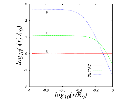
Figure 1: Radial density profile for the initial distribution of particles.

It should be noted that all the models to be presented in Section 2.6 have a total core mass of $M_{0}=5.41\,M_{\odot}$. Therefore, the particle masses $m_{i}$ are affected by a multiplicative constant, whose value obviously depends on the model in consideration. The value of the central density, $\rho_{c}$, is also affected. Thus, in Figure 1 we present the initial density profiles for the uniform and the two kinds of centrally condensed models considered here, as they were numerically measured from the initial snapshot.

2.2 The velocity of the particles

The velocity vector $\vec{v}(\vec{r})$ to be given to each SPH particle located at position $\vec{r}$ will be formed by the following combination of the two types of turbulent spectra, so that

$$\vec{v}(\vec{r})=\frac{1}{2}\,\vec{v}_{\rm DF}(\vec{r})+\frac{1}{2}\,\vec{v}_{\rm CF}(\vec{r})$$ (2)

The level of turbulence is adjusted by introducing a multiplicative constant in front of the right hand side of Eq. 2. It should be noted that Arreaga (2017) examined the effects on the collapse of cores due to variation of the number and size of the Fourier modes, although each turbulence type was allowed to act upon the core separately.

To generate the turbulent velocity spectrum, we set a second mesh, with a side length denoted here by $L_{0}$, which is proportional to the core radius $R_{0}$, so that

$$L_{0}=C_{R}\times R_{0}$$ (3)

where $C_{R}$ is a constant, the value of which will also determine the collapse model under consideration, see Section 2.6 and Table 1.

It must be noted that each term of Eq. 2 was calculated in Section 2.4 of Arreaga (2017), so that we do not repeat it here and show only the final expressions.

The components of the first term of Eq. 2 are given by

$$\begin{array}[]{l}\vec{v}_{\rm DF}\,\approx\Sigma_{i_{x},i_{y},i_{z}}\left|\vec{K}\right|^{\frac{-n-2}{2}}\times\par\left\{\par\begin{array}[]{l}\left[K_{z}\,C_{K_{y}}\sin\left(\vec{K}\cdot\vec{r}+\Phi_{K_{y}}\right)-K_{y}\,C_{K_{z}}\sin\left(\vec{K}\cdot\vec{r}+\Phi_{K_{z}}\right)\right]\;\mbox{for}\,v_{x}\\ \left[-K_{x}\,C_{K_{z}}\sin\left(\vec{K}\cdot\vec{r}+\Phi_{K_{z}}\right)+K_{z}\,C_{K_{x}}\sin\left(\vec{K}\cdot\vec{r}+\Phi_{K_{x}}\right)\right]\;\mbox{for}\,v_{y}\\ \left[-K_{x}\,C_{K_{y}}\sin\left(\vec{K}\cdot\vec{r}+\Phi_{K_{y}}\right)+K_{y}\,C_{K_{x}}\sin\left(\vec{K}\cdot\vec{r}+\Phi_{K_{x}}\right)\right]\;\mbox{for}\,v_{z}\\ \end{array}\par\right.\end{array}$$ (4)

see Dobbs et al. (2005). For the second term of Eq. 2 we have

$$\vec{v}_{\rm CF}(\vec{r})\approx\Sigma_{i_{x},i_{y},i_{z}}\left|\vec{K}\right|^{\frac{-n-2}{2}}\;\vec{K}\sin\left(\vec{K}\cdot\vec{r}+\Phi_{K}\right)$$ (5)

where the spectral index $n$ has been fixed in all our simulations to $n=-1$.

In the literature on turbulence, a parameter $\xi\in$ [0,1] is introduced to determine the relative contribution of the divergence-free and curl-free turbulent modes to the velocity field, see Federrath et al. (2010) and Brunt et al. (2014). According to equation 61 of Brunt et al. (2014), the value $\xi=$1/2, as the one chosen in this paper, implies that the ratio of curl-free power to total power of the velocity field is given by 1/3. Lomax et al. (2015) used the parameter $\delta_{\rm sol}$ that characterize the ratio of turbulent energy in diverge-free turbulent modes to the total turbulent energy, so that their model 2 defined by a velocity field given by $\vec{v}_{\rm DF}+\vec{v}_{\rm CF}$ has $\delta_{\rm sol}=$2/3, which is called a thermal mixture of turbulent modes. As we mentioned earlier, the velocity combination of this paper shown in Eq. 2, can be compared to model 2 of Lomax et al. (2015).

2.3 Initial energies

The relevant energies are calculated using all the SPH particles as follows:

$$\begin{array}[]{l}E_{\rm ther}=\frac{3}{2}\sum_{i}\,m_{i}\frac{P_{i}}{\rho_{i}}\\ E_{\rm kin}=\frac{1}{2}\sum_{i}\,m_{i}v_{i}^{2},\\ E_{\rm grav}=\frac{1}{2}\sum_{i}\,m_{i}\Phi_{i}\end{array}$$ (6)

where $P_{i}$ and $\Phi_{i}$ are the values of the pressure and gravitational potential at the location of particle $i$, with velocity given by $v_{i}$ and mass $m_{i}$; the summations include all the simulation particles.

In this paper, the value of the speed of sound $c_{0}$ is chosen in each model so that the simulations have

$$\frac{E_{\rm ther}}{\left|E_{\rm grav}\right|}\equiv 0.24$$ (7)

It should be noted that there are three different values of the speed of sound, see column 6 of Table 1. Thus, the corresponding temperatures associated with the core are $T\approx 3,4,7\,$K, respectively. It should be mentioned that Goodwin et al. (2004a) used a value of $\frac{E_{\rm ther}}{\left|E_{\rm grav}\right|}\equiv$ 0.45.

The level of turbulence is chosen to get the maximal value of $\frac{E_{\rm kin}}{E_{\rm grav}}$ in each model (see Section2.6 and Table 1), so that this is the maximum value for core collapse. In Section 2.6, we will explain how the values of $\left(\frac{E_{\rm kin}}{E_{\rm grav}}\right)_{\rm max}$ are obtained.

It must be mentioned that the virial theorem for a closed system in thermodynamic equilibrium can be expressed by the following relation:

$$\frac{E_{\rm ther}}{E_{\rm grav}}+\frac{E_{\rm kin}}{E_{\rm grav}}=\frac{1}{2}\;,$$ (8)

It should be mentioned that these energy ratios play a significant role in the determination of the stability of a gaseous system against gravitational perturbations. According to the virial theorem, if a gaseous system has $\frac{E_{\rm ther}}{E_{\rm grav}}+\frac{E_{\rm kin}}{E_{\rm grav}}>1/2$, then it will expand; in the other case, if $\frac{E_{\rm ther}}{E_{\rm grav}}+\frac{E_{\rm kin}}{E_{\rm grav}}<1/2$, then the system will collapse. Miyama et al. (1984), Hachisu and Heriguchi (1984) and Hachisu and Heriguchi (1985) obtained a more precise criterion of the type $\frac{E_{\rm ther}}{E_{\rm grav}}\times\frac{E_{\rm kin}}{E_{\rm grav}}<0.2$ to predict the collapse and fragmentation of a rotating isothermal core.

2.4 Evolution Code

The gravitational collapse of our models has been followed by using the fully parallelized particle-based code Gadget2; see Springel (2005) and also Springel et al. (2001). Gadget2 is based on the tree-PM method for computing the gravitational forces and on the standard smoothed particle hydrodynamics (SPH) method for solving the Euler equations of hydrodynamics. Gadget2 implements a Monaghan–Balsara form for the artificial viscosity; see Monaghan and Gingold (1983) and Balsara (1995). The strength of the viscosity is regulated by the parameter $\alpha_{\nu}=0.75$ and $\beta_{\nu}=\frac{1}{2}\,\times\alpha_{v}$; see Eqs. 11 and 14 in Springel (2005). In our simulations we fixed the Courant factor to be $0.1$.

2.5 Resolution and equation of state

The reliability of a program in calculating the collapse is determined by the resolution needed, which can be expressed in terms of the Jeans wavelength $\lambda_{J}$:

$$\lambda_{J}=\sqrt{\frac{\pi\,c^{2}}{G\,\rho}}\;,$$ (9)

where $c$ is the instantaneous speed of sound and $\rho$ is the local density; or to obtain a more useful form for a particle based code, the Jeans wavelength $\lambda_{J}$ can be transformed into a Jeans mass, given by

$$M_{J}\equiv\frac{4}{3}\pi\;\rho\left(\frac{\lambda_{J}}{2}\right)^{3}=\frac{\pi^{\frac{5}{2}}}{6}\frac{c^{3}}{\sqrt{G^{3}\,\rho}}\;.$$ (10)

where the values of the density and speed of sound must be updated according to the following equation of state:

$$p=c_{0}^{2}\,\rho\left[1+\left(\frac{\rho}{\rho_{crit}}\right)^{\gamma-1}\,\right],$$ (11)

which was proposed by Boss et al. (2000), where $\gamma\,\equiv 5/3$ and for the critical density we assume the value $\rho_{crit}=5.0\times 10^{-14}\,$ g   cm^-3.

Thus, the smallest mass particle that a SPH calculation must resolve in order to be reliable is given by $m_{r}\approx M_{J}/(2N_{\rm neigh})$, where $N_{\rm neigh}$ is the number of neighbouring particles included in the SPH kernel; see Truelove et al. (1997) and Bate and Burkert (1997). Hence, a simulation satisfying all the resolution requirements must satisfy $\frac{m_{p}}{m_{r}}<1$.

For the turbulent core under consideration, the number of particles is $N_{p}$ = 10,034,074, so that the average particle mass is given by m_p=5.3 $\times\,10^{-7}\,$ M_⊙. In addition, the number of neighboring particles is $N_{\rm neigh}=40$.

Let us first consider the U models, with the smallest value of the speed of sound, as given in Table 1, and assume that the peak density of these simulations to be used in this resolution calculation is $\rho=2.5\times 10^{-12}$ g cm^-3, then $M_{j}\approx 4.8\times 10^{-5}\,$ M_⊙ and m${}_{r}\approx 6\times 10^{-7}\,$ M_⊙. In this case, the ratio of masses is given by $m_{p}/m_{r}=$0.885 and then the desired resolution is achieved in these simulations up to this level of peak density. For the C models and assuming a peak density of $\rho=1.0\times 10^{-11}$ g cm^-3, we have $M_{j}\approx 4\times 10^{-5}\,$ M_⊙ and m${}_{r}\approx 5\times 10^{-7}\,$ M_⊙, so that $m_{p}/m_{r}=$1.0. Now consider the R models, which have the largest value of the sound speed, as given in Table 1, and again $\rho=2.5\times 10^{-11}$ g cm^-3, then $M_{j}\approx 8.5\times 10^{-5}\,$ M_⊙ and m${}_{r}\approx 1.6\times 10^{-6}\,$ M_⊙. In this case, the ratio of masses is given by $m_{p}/m_{r}=$0.5 and again the desired resolution is achieved in these simulations.

2.6 The models and their calibration

It must be mentioned that the values of the ratio $\left(\frac{E_{\rm kin}}{E_{\rm grav}}\right)_{\rm max}$, defined in Section 2.3, were determined by using an iterative process, so that for a given value of $\frac{E_{\rm kin}}{E_{\rm grav}}$, it was verified that the model collapses, otherwise a new value of $\frac{E_{\rm kin}}{E_{\rm grav}}$, higher than the previous one, was used until the model no longer collapses.

A clarification is needed to understand this calibration process of the models. As was mentioned in Section 2.2, in order to determine the particle velocity, a Fourier mesh of $N_{g}$ elements per side was used to generate the turbulent modes; this implies the calculation of $3\times N_{p}\,\times\,N_{g}^{3}$ operations where $N_{p}$ is the total number of particles, see Section 2.5. Therefore, at least $6.3\times 10^{13}$ operations must be performed to determine the velocity field of a simulation.

Our initial conditions code was parallelized in the number of particles, so that a processor takes only a fraction of the total $N_{p}$ particles to compute their velocities. Running in 80 processors in the cluster Intel Xeon E5-2680 v3 at 2.5 Ghz of LNS-BUAP, this code takes up to 8 hours to generate the initial conditions of all the simulation particles.

In such a situation, it is almost impractical to make the calibration of the models using all the simulation particles. For this reason, test models of a very few thousand particles were used, but only to determine the $\frac{E_{\rm ther}}{E_{\rm grav}}$ and $\left(\frac{E_{\rm kin}}{E_{\rm grav}}\right)_{\rm max}$ needed to calibrate each model.

The important point here is that it was verified that the values of $\frac{E_{\rm ther}}{E_{\rm grav}}$ and $\frac{E_{\rm kin}}{E_{\rm grav}}$ obtained in this test calibration do not change significantly in the complete simulation of $N_{p}$ particles. However, there is an indetermination factor $\delta$ in $\left(\frac{E_{\rm ther}}{E_{\rm grav}}\right)_{\rm max}$, so that it is expected that the turbulent core of the complete simulation is still in the collapsing regime within the range $\left(\frac{E_{\rm kin}}{E_{\rm grav}}\right)_{\rm max}\pm\delta$. In this paper, the upper bound of $\delta$ is less than (or equal to) 0.1.

The models considered in this paper are summarized in Table 1, whose entries are as follows. Column 1 shows the model number; column 2 shows the value of the constant $C_{R}$ as defined in Eq. 3, which determines the size of the Fourier mesh; column 3 shows the maximal energy ratio $\left(\frac{E_{\rm kin}}{E_{\rm grav}}\right)_{\rm max}$ reached by the model; column 4 shows the average Mach number${\cal M}$ obtained from the initial snapshot; column 5 shows the speed of sound used for each model; column 6 shows the number of the figure of the resulting configuration, and finally, column 7 shows a comment about the type of configuration obtained.

3 Results

The results of each model are illustrated by a column density plot, in which all the particles are used in order to make a 3D rendered image taken at the last snapshot available for each model. A bar located at the bottom of each iso-density plot shows the range of values for the $log$ of the column density $\rho(t)$, calculated in code units by the program splash version $2.7.0$, see Price (2007). The density unit is given by uden=4.77 $\times 10^{-21}$, so that the average density in code units is $\rho_{0}$/uden = 1.29. The colour bar shows values typically in the range 0–9, so that the peak column density is 10${}^{9}\,\times$ uden = 4.77 $\times 10^{-12}$ g cm^-3.

It must be clarified that the vertical and horizontal axes of all the iso-density plots indicate the length in terms of the radius $R_{0}$ of the core (approximately 3335 AU). So, the Cartesian axes $X$ and $Y$ vary initially from -1 to 1. However, in order to facilitate the visualization of the last configuration obtained, we do not use the same length scale per side in all the plots.

3.1 Dynamical evolution: A general picture

We now briefly describe, in general terms, the time evolution of the core as seen by using the publicly available visualization code splash, see Price (2007).

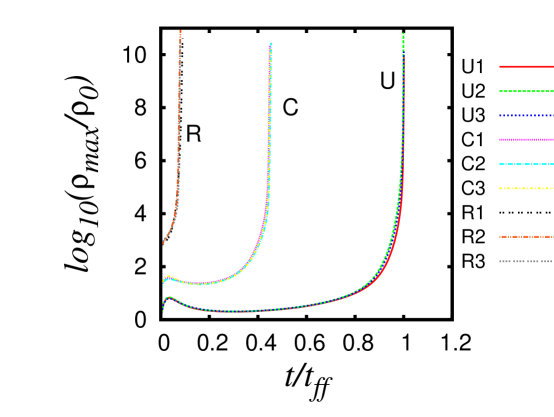
Figure 2: Time evolution of the peak density $\rho_{max}$ of the models U, C and R. The curves overlap.

A turbulent velocity field favours the occurrence of collisions between particles across the entire core volume. We decided to include the turbulence only at the initial simulation time and to leave the core to collapse freely, so that the first evolution stage is characterized by an early increase in the peak density, which can be seen in the first part of the curves for the U and C models shown in Fig. 2. After this density rebound, the core truly begins its collapse, because the initial kinetic energy of the turbulence velocity field was already dissipated.

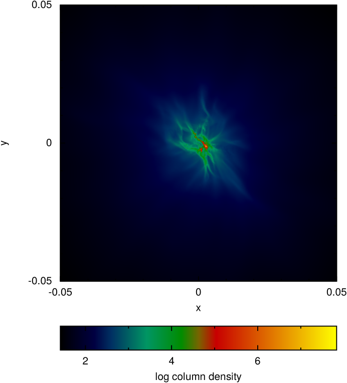
Figure 3: Column-density plot of the central $(-0.05/R_{0},0.05/R_{0})$ core X-Y midplane for model U1 when $\rho_{\rm max}=5.7\times 10^{-11}$ g/cm³ and $t/t_{ff}=1.0$.

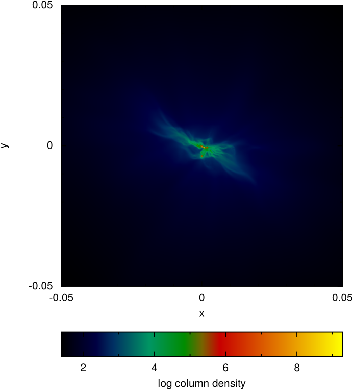
Figure 4: Column-density plot of the central $(-0.05/R_{0},0.05/R_{0})$ core X-Y midplane for model U2 when $\rho_{\rm max}=4.1\times 10^{-10}$ g/cm³ and $t/t_{ff}=0.99$.

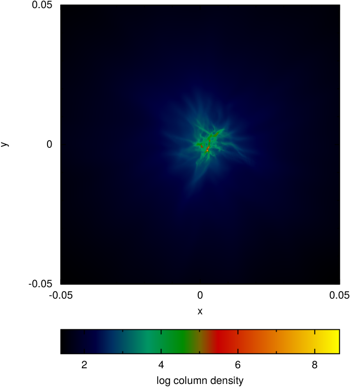
Figure 5: Column-density plot of the central $(-0.05/R_{0},0.05/R_{0})$ core X-Y midplane for model U3 when $\rho_{\rm max}=9.7\times 10^{-11}$ g/cm³ and $t/t_{ff}=1.0$.

For the uniform models, it can be seen that many dense gas filaments are formed at the central region of the core. Some of them show fragmentation, so that a few protostars are in their way of formation, see Fig. 3. When the wavelength of the perturbation mode increases to $4\times R_{0}$, it can be seen that one direction is dominant, along which the filaments form, see Fig. 4. In the case of model U3, the central overdensity seems to be a little bit elongated, see Fig. 5.

The density rebound, characterizing the first stage of evolution is not visible in the peak density curves of models R. The reason for this is that, at time $t=0$, all the particles are uniformly distributed across the entire core volume; for the uniform models, all the particles have the same mass, whereas for the centrally condensed models, those particles located in the innermost central region have larger masses than those located in the outermost core. The collapse is thus stronger and quicker in the central region of the centrally condensed core.

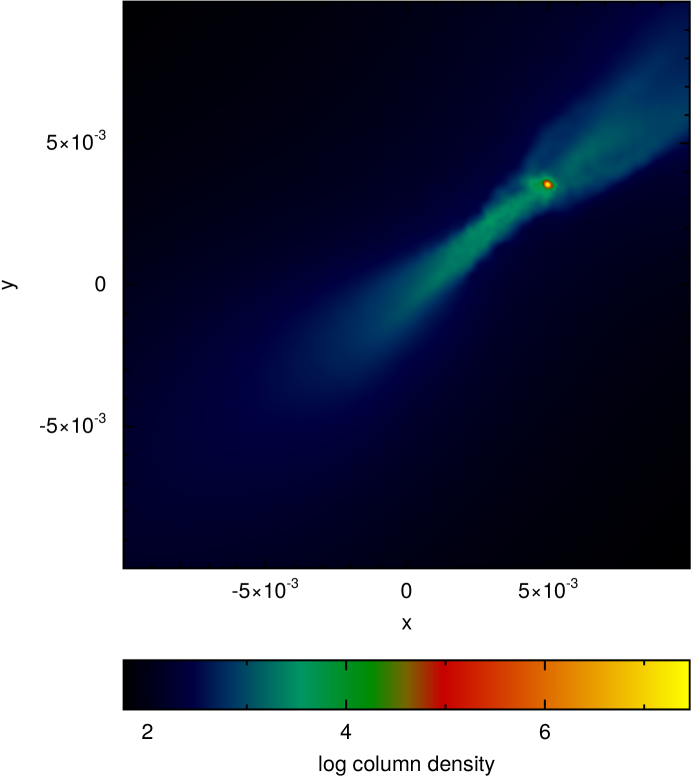
Figure 6: Column-density plot of the central $(-0.01/R_{0},0.01/R_{0})$ core X-Y midplane for model C1 when $\rho_{\rm max}=1.8\times 10^{-10}$ g/cm³ and $t/t_{ff}=0.449$.

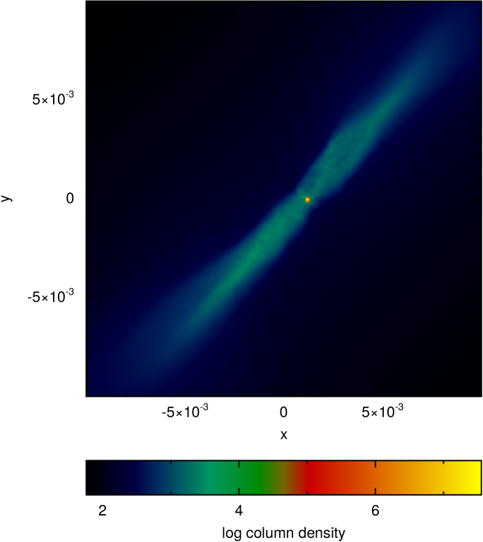
Figure 7: Column-density plot of the central $(-0.01/R_{0},0.01/R_{0})$ core X-Y midplane for model C2 when $\rho_{\rm max}=1.69\times 10^{-10}$ g/cm³ and $t/t_{ff}=0.454$.

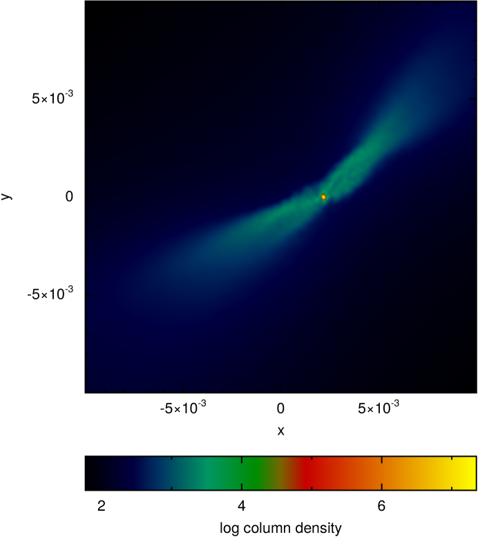
Figure 8: Column-density plot of the central $(-0.01/R_{0},0.01/R_{0})$ core X-Y midplane for model C3 when $\rho_{\rm max}=1.04\times 10^{-10}$ g/cm³ and $t/t_{ff}=0.45$.

For the C models, we observe mainly the formation of a long filament, inside which there is a well-defined overdensity in the central region of the core, so in these models, the collapse of the core will form only a primary protostar inside a gas filament, see Fig. 6, Fig. 7 and Fig. 8.

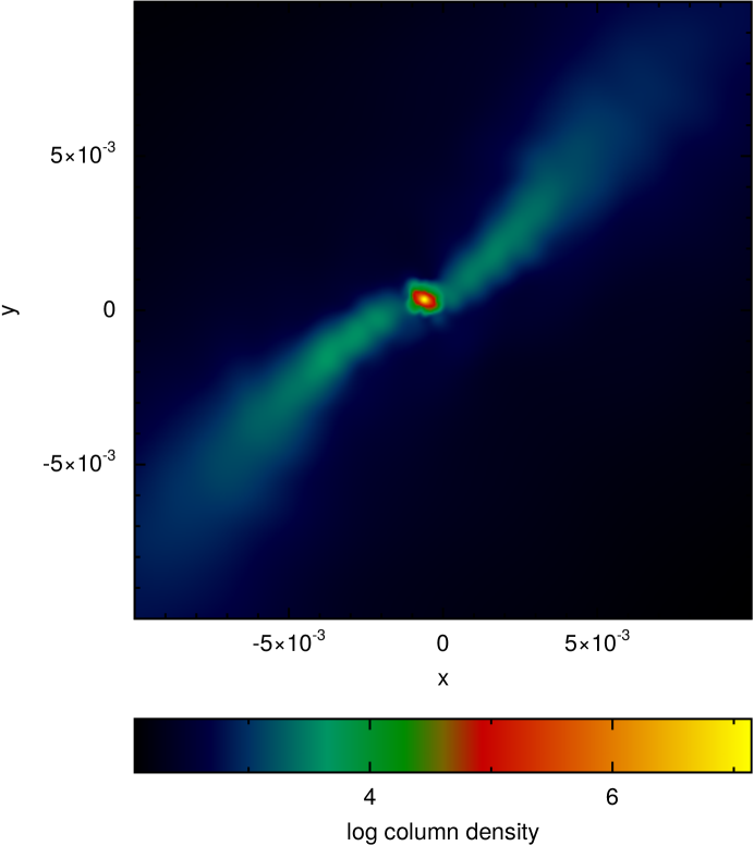
Figure 9: Column-density plot of the central $(-0.01/R_{0},0.01/R_{0})$ core X-Y midplane for model R1 when $\rho_{\rm max}=2.5\times 10^{-10}$ g/cm³ and $t/t_{ff}=0.09$.

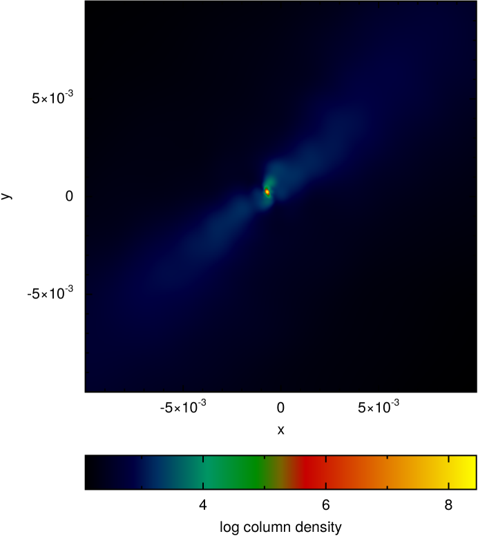
Figure 10: Column density plot of the central $(-0.01/R_{0},0.01/R_{0})$ core X-Y midplane for model R2 when $\rho_{\rm max}=1.9\times 10^{-9}$ g/cm³ and $t/t_{ff}=0.08$.

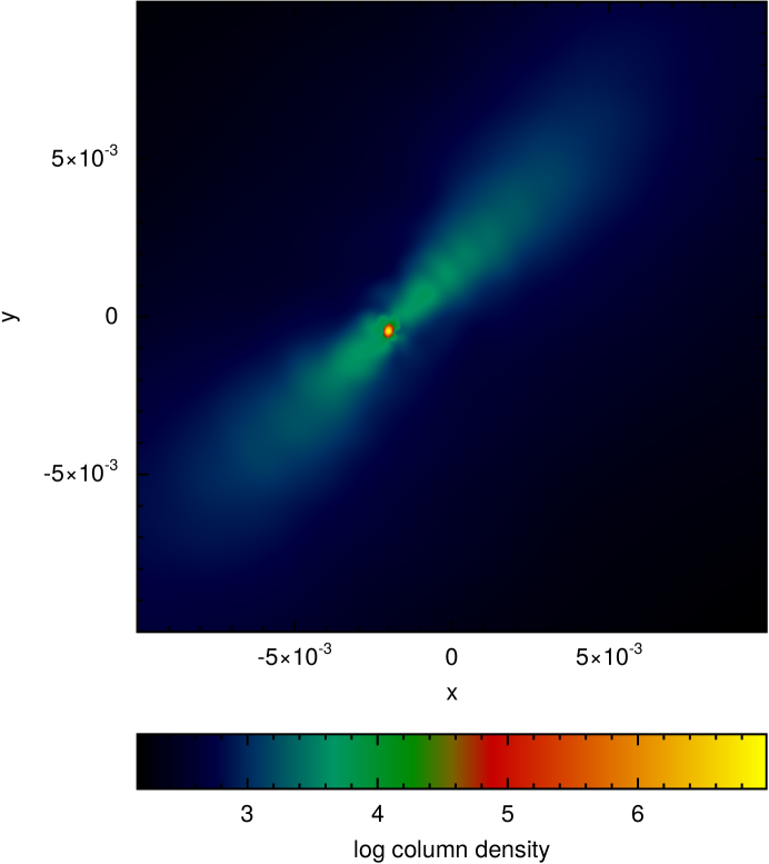
Figure 11: Column-density plot of the central $(-0.01/R_{0},0.01/R_{0})$ core X-Y midplane for model R3 when $\rho_{\rm max}=2.0\times 10^{-10}$ g/cm³ and $t/t_{ff}=0.08$.

In the case of R models, the central region of the core accretes much more mass very rapidly and thus the collapse takes place more rapidly in the central region, so that the mentioned filament could have a net angular momentum, see and compare Fig. 9, Fig. 10 and Fig. 11.

For all the centrally condensed models, the central collapse is so strong that the increase of the wavelength of the perturbation mode does not affect significantly the basic configuration.

3.2 Physical properties

In order to calculate some physical properties of the resulting protostars, such as the mass and the values of the energy ratios $\left(\frac{E_{\rm ther}}{E_{\rm grav}}\right)_{f}$ and $\left(\frac{E_{\rm kin}}{E_{\rm grav}}\right)_{f}$, we used a subset of the simulation particles, which are determined by means of the following procedure. First, the highest density particle of the last available snapshot for each model was located; this particle is going to be the centre of the protostar. All those particles are found that (i) have density above some minimum value fixed beforehand $\log_{10}\left(\rho_{\rm min}/\rho_{0}\right)=2.0$ for all the turbulent models and (ii) are also located within a given maximum radius $r_{\rm max}$ from the protostar’s centre.

The physical properties thus obtained are reported in Table 2, whose entries are as follows. The first column shows the number and label of the model; the second column shows the parameter $r_{\rm max}$ given in terms of the core radius $R_{0}$; the third column shows the number of particles used in the calculation of the properties; the fourth column shows the mass of the resulting protostar given in terms of $M_{\odot}$; the fifth and sixth columns give the values of $\left(\frac{E_{\rm ther}}{E_{\rm grav}}\right)_{f}$ and $\left(\frac{E_{\rm kin}}{E_{\rm grav}}\right)_{f}$, respectively.

Many lines are included in the Table 2 as protostars have been found in each uniform model, so that the properties of different protostars are referred to in different lines of Table 2. The average separation of the protostar found in the uniform models is around 23 to 29 AU (astronomical units).

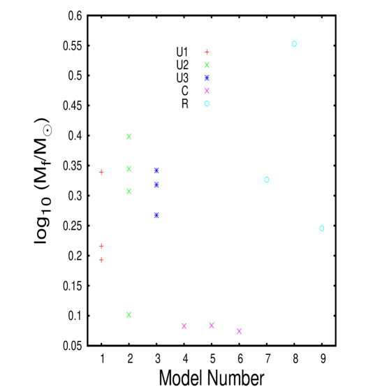
Figure 12: Fragment masses against the model number; see Table 2.

In Fig. 12, the masses of the protostars are shown in terms of the model number. For the U models, the masses ranges within 0.2-0.4 $M_{\odot}$. For C models, the masses are less than 0.1 $M_{\odot}$. As expected, the largest protostar mass was found for one of the R models.

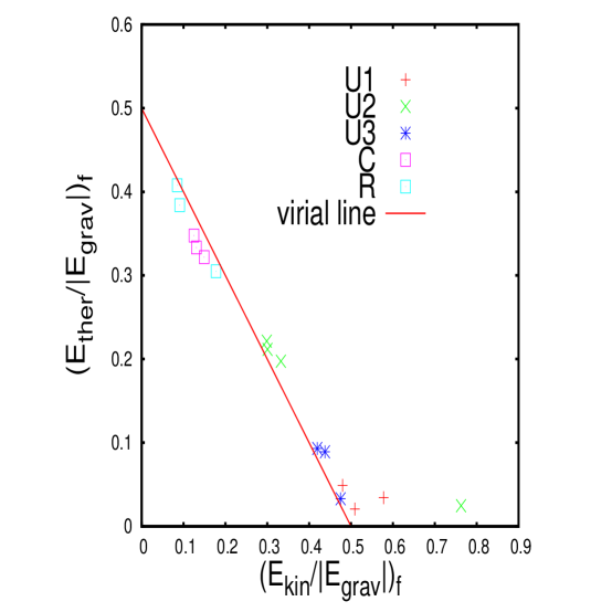
Figure 13: Integral properties of protostars: the vertical axis is the ratio of the thermal energy to the gravitational energy and the horizontal axis is the ratio of the kinetic energy to the gravitational energy; see columns 5 and 6 of Table 2.

It must be mentioned that the values obtained for the energy ratios of the protostars, namely $\left(\frac{E_{\rm ther}}{E_{\rm grav}}\right)_{f}$ and $\left(\frac{E_{\rm kin}}{E_{\rm grav}}\right)_{f}$, unfortunately depend on the values chosen for the parameters $\rho_{\rm min}$ and $r_{\rm max}$, as there is an ambiguity in defining the boundaries of the protostar. Despite this, the values of $\left(\frac{E_{\rm ther}}{E_{\rm grav}}\right)_{f}$ and $\left(\frac{E_{\rm kin}}{E_{\rm grav}}\right)_{f}$ for the C models show a clear tendency to virialize, as can be appreciated in Fig. 13. This behavior is to be expected, as the collapse of these models was so strongly centrally dominated that the formed protostars reach very quickly a thermal support against gravity. We emphasize that a similar observation was made by  Arreaga and Saucedo (2012).

4 Discussion

In this paper, we have studied the nature of the gravitational collapse of a core when extreme values of kinetic energy are provided initially by means of several turbulent velocity fields.

In order to make this paper of interest for star formation, in spite of the fact that these high values of $\left(\frac{E_{\rm kin}}{E_{\rm grav}}\right)_{\rm max}$ are perhaps unrealistic initial conditions in the observational sense, we always focused on collapsing cores and so we thus showed that the parameter space of $\frac{E_{\rm kin}}{E_{\rm grav}}$ is enormous. Indeed, in Section 2.6 we explained in detail the calibration process of our models in order to obtain the maximal value of $\left(\frac{E_{\rm kin}}{E_{\rm grav}}\right)_{\rm max}$ allowed in a collapsing core, namely: we always checked the occurrence of the collapse of the core before we increased the value of $\left(\frac{E_{\rm kin}}{E_{\rm grav}}\right)_{\rm max}$, so when the core did not collapse anymore, the process was stopped.

According to Fig. 14, where we show the $\left(\frac{E_{\rm kin}}{E_{\rm grav}}\right)_{\rm max}$ obtained for each model against the central density of the core ( see also column 3 of Table 1), the uniform models can manage a very high input of initial energy, which is dissipated by means of particle collisions, so that the collapse takes place around a 1 free fall time $t_{ff}$, see Fig. 2. At the opposite extreme, the centrally condensed models need much less input of initial energy, so that their collapse take place very quickly: for instance the collapse time for C models ranges around 0.45 times $t_{ff}$, while for R models, the collapse time varies within 0.08-0.09 times $t_{ff}$.

This behavior is to be expected, as the local free-fall time of C and R models in the innermost region of the core are shorter than in the outermost region. In these cases, we observed the occurrence of the so-called inside-out gas collapse, in which the central region of the core collapses first while much gas is left behind with low levels of collapse in the core outer region.

It should be noted that the values thus obtained for $\left(\frac{E_{\rm kin}}{E_{\rm grav}}\right)_{\rm max}$ (recall that $\frac{E_{\rm ther}}{E_{\rm grav}}$ was fixed for all the models ) were so high that the collapse of the core would not be expected, because the sum of the values chosen for the initial energy ratios $\frac{E_{\rm ther}}{E_{\rm grav}}$ and $\left(\frac{E_{\rm kin}}{E_{\rm grav}}\right)_{\rm max}$ is always higher than the equilibrium value given in Eq. 8, and therefore these ratios would not favour in principle the global collapse of the core, see Section 2.3. Two clarifying comments are in order concerning the high values of $\left(\frac{E_{\rm kin}}{E_{\rm grav}}\right)_{\rm max}$.

Firstly, it must be taken into account that the virial theorem of Section 2.3 does not include the effects of turbulence on the dynamics of the core, namely, that many gas collisions take place simultaneously across the core in the initial stage of the simulation, so that the gas is simultaneously compressed in many places, favouring the local collapse of the core. In fact, early theoretical attempts to take into account this particular nature of turbulence in the task of predicting the fate of a turbulent gas system were made by Sasao (1973) and Bonazzola (1987), who suggested considering a wavenumber-dependent effective speed of sound, so that $c_{0}\equiv c_{0}(K)$. Because of this issue, it is also possible that the resolution analysis presented in Section 2.5 is incomplete, in the sense that a Jeans mass $M_{J}$ must be replaced as well by an effective Jeans mass $M_{J}\equiv M_{J}(K)$.

Secondly, observational values of $\frac{E_{\rm kin}}{E_{\rm grav}}$ for prestellar cores have been found to be within the range 10^-4 to 0.07, see Caselli et al. (2002) and Jijina (1999). It thus seems that the high values of $\frac{E_{\rm kin}}{E_{\rm grav}}$ of this paper are not physically justified. This is a very important point, but it must be mentioned that the initial conditions for the standard isothermal test case calculated by Boss and Bodenheimer (1979), Boss (1991), Truelove et al (1998),Klein et al. (1999), Boss et al. (2000), and Kitsionas & Whitworth (2002), among others, were $\frac{E_{\rm ther}}{\left|E_{\rm grav}\right|}=0.26$ and $\frac{E_{\rm kin}}{\left|E_{\rm grav}\right|}=0.16$.

A possible limitation of the models presented in this paper is that we did not use the sink technique introduced by Bate et al. (1995) and later updated by Federrath et al. (2010), so that our simulations did not evolve much further in time than when the collapse occurred. If we were able to follow the simulations longer, we could possibly see the fragmentation of the filament of some primary protostars.

A final consideration to be mentioned here is that the stochastic nature of the turbulent spectrum of the velocity field was not taken into account, namely, in this paper, the seed to generate the random numbers was the same for all simulations and it was fixed from the beginning. However, it has been shown elsewhere that simulations with different realizations of the random seeds can have significant differences in their outcomes; see for instance Walch et al. (2012), Girichidis et al. (2011), Federrath and Klessen (2012), who used different random seeds to make a suite of turbulent simulations.

5 Concluding Remarks

In this paper we carefully prepared the initial conditions for the particles in order to have a collapsing core and thus we bounded the value of $\left(\frac{E_{\rm kin}}{E_{\rm grav}}\right)_{\rm max}$ for each model, so that beyond this value of $\frac{E_{\rm kin}}{E_{\rm grav}}$, the core get dispersed unboundedly. We emphasized that the total mass and radius of the core are the same for all the models, so that we changed only (i) the radial density profile and (ii) the wavelength of the perturbation mode.

The main result of this paper is therefore shown in Fig.14, in which we observed that (i) less input of kinetic energy is required to disperse the core as the central density increases; (ii) the effect of the increase in the wavelength of the perturbation mode is very small.

We obtained interesting configurations at the end of the core collapse, particularly those of models 1-3, which showed multiple fragmentation mainly along filaments. Lomax et al. (2015) studied a total of 50 models of velocity fields for core collapse in which the turbulent energy was varied, and identified two principal modes of fragmentation, namely the filament fragmentation and disk fragmentation. It must be noted that configurations of models 1-3 of this paper, correspond to the filament fragmentation mode.

In addition, the centrally condensed models resulted in the formation of a single central protostar, which is inside a long filament. Fragmentation was perhaps suppressed by the extreme mass concentration at the centre of the core.

Table 1: Turbulent models and their resulting configurations

Model Number (label)	$C_{R}$	$\left(\frac{E_{\rm kin}}{\left|E_{\rm grav}\right|}\right)_{\rm max}$	${\cal M}_{\rm ave}$	$c_{0}$ [cm/s]	Figure	Configuration
1 (U1)	1	8.4	8.96	9677.64	3	primary + fragmented filaments
2 (U2)	4	9.4	9.45	9677.64	4	fragmented filaments
3 (U3)	10	8.9	9.24	9677.64	5	fragmented filaments
4 (C1)	1	2.96	5.38	11423.37	6	single + long filament
5 (C2)	4	3.09	5.49	11423.37	7	single + long filament
6 (C3)	10	2.96	5.37	11423.37	8	single + long filament
7 (R1)	1	1.27	3.63	17097.9	9	single + long filament
8 (R2)	4	0.9	3.05	17097.9	10	single + long filament
9 (R3)	10	1.03	3.2	17097.9	11	single + long filament

Table 2: Integral properties of protostars

Model Number (label)	r${}_{\rm max}/R_{0}$	$N_{p}$	$M_{f}/M_{\odot}$	$\left(\frac{E_{\rm ther}}{\left|E_{\rm grav}\right|}\right)_{f}$	$\left(\frac{E_{\rm kin}}{\left|E_{\rm grav}\right|}\right)_{f}$
1 (U1)	0.008	628984	3.39e-01	0.049	0.479
1 (U1)	0.008	400546	2.16e-01	0.020	0.509
1 (U1)	0.008	358062	1.93e-01	0.034	0.578
2 (U2)	0.008	739098	3.98e-01	0.197	0.333
2 (U2)	0.008	639297	3.45e-01	0.211	0.300
2 (U2)	0.008	570112	3.07e-01	0.221	0.299
2 (U2)	0.008	188238	1.01e-01	0.025	0.762
3 (U3)	0.008	634095	3.42e-01	0.089	0.438
3 (U3)	0.008	589909	3.18e-01	0.093	0.419
3 (U3)	0.008	495728	2.67e-01	0.033	0.475
4 (C1)	0.005	15187	8.28e-02	0.322	0.149
5 (C2)	0.005	15419	8.39e-02	0.348	0.125
6 (C3)	0.005	13450	7.41e-02	0.333	0.130
7 (R1)	0.005	2514	3.27e-01	0.305	0.178
8 (R2)	0.005	4310	5.52e-01	0.408	0.085
9 (R3)	0.005	1666	2.46e-01	0.384	0.090

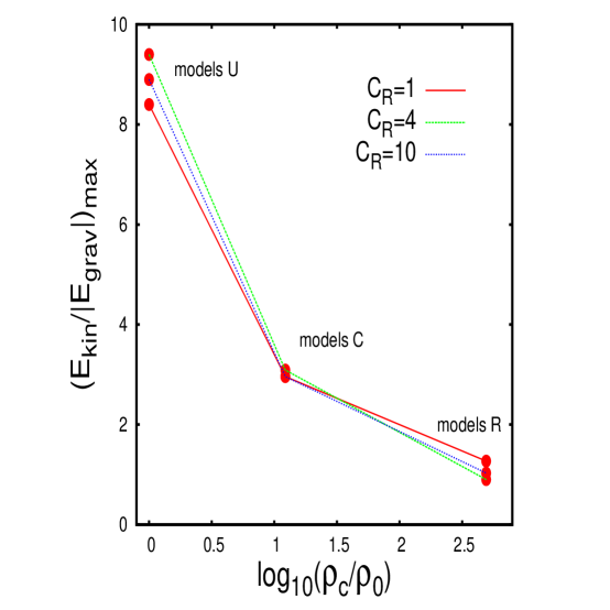
Figure 14: The value of $\left(\frac{E_{\rm kin}}{E_{\rm grav}}\right)_{\rm max}$ against the central density of the core (normalized to the average density of the core $\rho_{0}$). The lines join models with the same wavelength of the perturbation mode and the points show the measurements made in this paper.

References

- André (2007) André P., Belloche, A., Motte, F. and Peretto, N., 2007, Astron. Astrophys., 472, 519.
- Arreaga et al. (2009) Arreaga, G., Klapp, J. and Gomez, F., 2009, Astron. Astrophys., 509, pp. A96–A111.
- Arreaga et al. (2007) Arreaga, G., Klapp, J.,Sigalotti L.D., Gabbasov, R., 2007, ApJ, 666, 290–.
- Arreaga and Saucedo (2012) Arreaga-García, G. and Saucedo-Morales, J.C., 2012, Revista Mexicana de Astronomía y Astrofísica, 48, pp. 61–84.
- Arreaga (2016) Arreaga-García, G., 2016, Revista Mexicana de Astronomía y Astrofísica, 52, pp. 155–169.
- Arreaga (2017) Arreaga-García, G., 2017, Astrophysics and Space Science 362, pp. 47–.
- Arreaga (2017) Arreaga-García, G., 2017, Revista Mexicana de Astronomía y Astrofísica, 53, pp. 1–24.
- Attwood et al. (2009) Attwood, R.E., Goodwin, S.P., Stamatellos, D. and Whitworth, A.P., 2009, Astron. Astrophys., 495, pp. 201–215.
- Ballesteros et al. (1999) Ballesteros-Paredes, J., Hartmann, L. and Vazquez-Semanedi, E., 1999, ApJ, 527, pp. 285.
- Balsara (1995) Balsara, D., 1995, J. Comput. Phys., 121, 357.
- Bate et al. (1995) Bate, M.R., Bonnell, I.A. and Price, N.M., 1995, MNRAS, 277, pp. 362–376.
- Bate et al. (2002a) Bate, M.R., Bonnell, I.A. and Bromm, V., 2002, MNRAS, 332, pp. L65–L68.
- Bate et al. (2002b) Bate, M.R., Bonnell, I.A. and Bromm, V., 2002, MNRAS, 336, pp. 705–713.
- Bate et al. (2003) Bate, M.R., Bonnell, I.A. and Bromm, V., 2003, MNRAS, 339, pp. 577–599.
- Bate and Burkert (1997) Bate, M.R. and Burkert, A., 1997, MNRAS, 288, 1060.
- Bergin et al. (2007) Bergin, E. and Tafalla, M., 2007, Annu. Rev. Astro. Astrophys., 45, 339.
- Bodenheimer (1995) Bodenheimer, P., 1995, ARA&A, 33, 199.
- Bonazzola (1987) Bonazzola, S., Falgorone, E., Heyvaerts, J., Pérault, M., and Puget, J.L., 1987, Astron. Astrophys., 172, 293.
- Boss and Bodenheimer (1979) Boss, A.P. and Bodenheimer, P. 1979, ApJ, 234, 289.
- Boss (1980) Boss, A.P., 1980, ApJ, 242, pp. 699–709.
- Boss (1981) Boss, A.P., 1981, ApJ, 250, 636644.
- Boss (1991) Boss, A.P., 1991, Nature, 351, pp. 298.
- Brunt et al. (2014) Brunt, C.M. and Federrath, C., 2014, MNRAS, 442, 1451.
- Brunt et al. (2009) Brunt, C.M., Heyer, M.H. and MacLow, M.M., 2009, Astron. Astrophys., 504, 883.
- Bouwman (2004) Bouwman, A.P., 2004, Astrophysics and Space Science, 292, 325.
- Boss et al. (2000) Boss, A.P., Fisher, R.T., Klein, R. and McKee, C.F., 2000, ApJ, 528, 325.
- Burkert and Bodenheimer (1993) Burkert, A. and Bodenheimer, P., 1993, MNRAS, 264, 798.
- Caselli et al. (2002) Caselli, P., Benson, P.J., Myers, P.C. and Tafalla, M., 2002, ApJ, 572, 238.
- Chandrasekhar (1951) Chandrasekhar, S., 1951, Proc. R. Soc. London, 210, 26.
- Dobbs et al. (2005) Dobbs, C.L., Bonnell, I.A. and Clark, P.C., 2005, MNRAS, 360, pp. 2–8.
- Elmegreen (1993) Elmegreen, B.G., 1993, in: Protostars and Planets III, pp. 97.
- Federrath (2015) Federrath, C.,2015, MNRAS, 450, Issue 4, p.4035-4042.
- Federrath et al. (2010) Federrath, C., Roman-Duval, J., Klessen, R.S., Schmidt, W. and Mac Low, M.M., 2010, Astron. Astrophys., 512, A81.
- Federrath et al. (2010) Federrath, C., Banerjee, R. Clark, P. C. and Klessen, R. S., 2010, ApJ, 713, Issue 1, pp. 269-290.
- Federrath and Klessen (2012) Federrath, C. and Klessen, R.S., 2012, ApJ,761, Issue 2, article id. 156.
- Girichidis et al. (2011) Girichidis, P., Federrath, C., Banerjee, R. and Klessen, R. S., 2011, MNRAS, 413, Issue 4, pp. 2741-2759.
- Goodman et al. (1993) Goodman, A.A., Benson, P.J., Fuller, G.A., Myers, P.C., 1993, ApJ, 406, pp. 528–547.
- Goodwin et al. (2004a) Goodwin, S.P., Whitworth, A.P. and Ward-Thompson, D., 2004a, Astron. Astrophys., 414, pp. 633–650.
- Goodwin et al. (2004b) Goodwin, S.P., Whitworth, A.P. and Ward-Thompson, D., 2004b, Astron. Astrophys., 423, pp. 169–182.
- Goodwin et al. (2006) Goodwin, S.P., Whitworth, A.P. and Ward-Thompson, D., 2006, Astron. Astrophys., 452, pp. 487–492.
- Hachisu and Heriguchi (1984) Hachisu, I. and Heriguchi, Y., 1984, Astron. Astrophys., 140, 259.
- Hachisu and Heriguchi (1985) Hachisu, I. and Heriguchi, Y., 1985, Astron. Astrophys., 143, 355.
- Hopkins (2013) Hopkins, F., 2013, MNRAS, 430, pp. 1653–1693.
- Jijina (1999) Jijina, J., Myers, P.C. and Adams, F.C., 1999, ApJ, 125, pp. 161–236.
- Klein et al. (1999) Klein, R. I., Fisher, R. T., McKee, C. F. and Truelove, J. K. 1999, in Numerical Astrophysics 1998, ed. S. Miyama, K. Tomisaka and T. Hanawa Kluwer, Dordrecht, pp. 131–.
- Kitsionas & Whitworth (2002) Kitsionas, S., Whitworth, A.P., 2002, MNRAS, 330, 129.
- Léorat (1990) Léorat, J., Passot, T. and Pouquet, A., 1990, MNRAS, 243, pp. 293–311.
- Lomax et al. (2015) Lomax, O., Whitworth, A.P., and Hubber, D.A., 2015, MNRAS, 449, pp.662-669.
- Myers (2005) Myers, P.C., 2005, ApJ, 623, 280.
- Miyama et al. (1984) Miyama, S.M., Hayashi, C. and Narita, S., 1984, ApJ, 279, 621.
- Monaghan and Gingold (1983) Monaghan, J.J. and Gingold, R.A., 1983, J. Comput. Phys., 52, 374.
- Padoan and Norlund (2002) Padoan, P. and Nordlund, A., 2002, ApJ, 576, pp. 870–879.
- Padoan et al. (2014) Padoan, P., Federrath, C., Chabrier, G., Evans II, N.J., Johnstone, D., Jrgensen, J.K., McKee, C.F. and Nordlund, E., 2014, Protostars and Planets VI, H. Beuther, R. S. Klessen, C. P. Dullemond, and T. Henning (eds.), University of Arizona Press, Tucson, AZ, pp. 77–100. arXiv. 1312.5365.
- Plummer (1911) Plummer, H.C., 1911, MNRAS, 71, 460.
- Sigalotti and Klapp (2001) Sigalotti, L. and Klapp, J., 2001, Int. J. Mod. Phys. D, 10, 115.
- Sasao (1973) Sasao, T., 1973, PASJ, 25, 1.
- Springel (2005) Springel, V., 2005, MNRAS, 364, 1105.
- Springel et al. (2001) Springel, V., Yoshida, N. and White, S.D.M., 2001, New Astronomy, 6, 79.
- Price (2007) Price, D., 2007, PASA 24(3), pp. 159–173. The code SPLASH was taken from http://users.monash.edu.au/ dprice/splash/, SPLASH: a free and open source visualisation tool for Smoothed Particle Hydrodynamics (SPH) simulations, 2015.
- Tafalla et al. (1998) Tafalla, M., Mardones, D. and Myers, P.C., 1998, ApJ, 504, pp. 900–914.
- Tafalla et al. (2004) M. Tafalla, M., Myers, P.C., Caselli, P. and Walmsley, C.M., 2004, Astron. Astrophys., 416, pp. 191–212.
- Tobin et al. (2012) Tobin, J.J, Hartmann, L. and Chiang, H.F., 2012, Nature, 492, 83.
- Tobin at al. (2013) Tobin, J.J., Chandler, C., Wilner, D.J., Looney, L.W., Loinard, L., Chiang, H.-F., Hartmann, L., Calvet, N., D’Alessio, P., Bourke, T.L. and Kwon, W., 2013, ApJ779.
- Tobin at al. (2016) Tobin, J.J., Kratter, K.M., Persson, M.V., Looney, L.W., Dunham, M.M., Segura-Cox, D., Li, Z.Y., Chandler, C.J., Sadavoy, S.I., Harris, R.J., Melis, C., and Pérez, L.M., 2016, Nature, 38, pp. 483–486.
- Tohline (2002) Tohline, J.E., 2002, ARA&A, 40, 349.
- Truelove et al. (1997) Truelove, J.K., Klein, R.I., McKee, C.F., Holliman, J.H., Howell, L.H. and Greenough, J.A., 1997, ApJ, 489, L179.
- Truelove et al (1998) Truelove, J. K., Klein, R. I., McKee, C. F., Holliman, J. H., Howell, L. H., Greenough, J. A. and Woods, D. T. 1998, ApJ, 495, 821.
- Tsuribe et al. (1999) Tsuribe, T. and Inutsuka, S.-I., 1999, ApJ523, pp. L155–L158. Tsuribe, T. and Inutsuka, S.-I., 1999, ApJ, 526, pp. 307–313.
- Walch et al. (2012) Walch, S., Whitworth, A.P. and Girichidis, P., 2012, MNRAS, 419, pp. 760–770.
- Whitehouse and Bate (2006) Whitehouse, S.C. and Bate, M.R., 2006, MNRAS, 367, 32.
- Whitworth and Ward-Thompson (2001) Whitworth, A.P. and Ward-Thompson, D., 2001, ApJ, 54, 317.