Probability measure characterization by $L^{p}$-quantization error function

Convergence Rate of Optimal Quantization and Application to the Clustering Performance of the Empirical Measure

Abstract

We study the convergence rate of the optimal quantization for a probability measure sequence $(\mu_{n})_{n\in\mathbb{N}^{*}}$ on $\mathbb{R}^{d}$ converging in the Wasserstein distance in two aspects: the first one is the convergence rate of optimal quantizer $x^{(n)}\in(\mathbb{R}^{d})^{K}$ of $\mu_{n}$ at level $K$; the other one is the convergence rate of the distortion function valued at $x^{(n)}$, called the “performance” of $x^{(n)}$. Moreover, we also study the mean performance of the optimal quantization for the empirical measure of a distribution $\mu$ with finite second moment but possibly unbounded support. As an application, we show that the mean performance for the empirical measure of the multidimensional normal distribution $\mathcal{N}(m,\Sigma)$ and of distributions with hyper-exponential tails behave like $\mathcal{O}(\frac{\log n}{\sqrt{n}})$. This extends the results from [BDL08] obtained for compactly supported distribution. We also derive an upper bound which is sharper in the quantization level $K$ but suboptimal in $n$ by applying results in [FG15].

keywords: Clustering performance, Convergence rate of optimal quantization, Distortion function, Empirical measure, Optimal quantization.

1 Introduction

The $K$-means clustering procedure in the unsupervised learning area was first introduced by [Mac67], which consists in partitioning a data set of observations $\{\eta_{1},...,\eta_{N}\}\subset\mathbb{R}^{d}$ into $K$ classes $\mathcal{G}_{k},{1\leq k\leq K}$ with respect to a cluster center $x=(x_{1},...,x_{K})$ in order to minimize the quadratic distortion function $\mathcal{D}_{K,\eta}$ defined by

$$x=(x_{1},...,x_{K})\in(\mathbb{R}^{d})^{K}\mapsto\mathcal{D}_{K,\eta}(x)\coloneqq\frac{1}{N}\sum_{n=1}^{N}\min_{k=1,...,K}d(\eta_{n},x_{k})^{2},$$ (1.1)

where $d$ denotes a distance on $\mathbb{R}^{d}$. The classification of the observations $\{\eta_{1},...,\eta_{N}\}\subset\mathbb{R}^{d}$ in [Mac67] can be described as follows

$$\mathcal{G}_{1}=\big{\{}\;\eta_{n}\in\{\eta_{1},...,\eta_{N}\}\;:\;d(\eta_{n},x_{1})\leq\min_{2\leq j\leq K}d(\eta_{n},x_{j})\;\big{\}}$$

$$\mathcal{G}_{2}=\big{\{}\;\eta_{n}\in\{\eta_{1},...,\eta_{N}\}\;:\;d(\eta_{n},x_{2})\leq\min_{1\leq j\leq K,j\neq 2}d(\eta_{n},x_{j})\;\big{\}}\setminus\mathcal{G}_{1}$$

$$\cdots$$

$$\mathcal{G}_{K}=\big{\{}\;\eta_{n}\in\{\eta_{1},...,\eta_{N}\}\;:\;d(\eta_{n},x_{K})\leq\min_{1\leq j\leq K-1}d(\eta_{n},x_{j})\;\big{\}}\setminus\big{(}\mathcal{G}_{K-1}\cup\cdots\cup\mathcal{G}_{1}\big{)}.$$ (1.2)

If a cluster center $x^{*}=(x^{*}_{1},...,x^{*}_{K})$ satisfies $\mathcal{D}_{K,\eta}(x^{*})=\inf_{y\in(\mathbb{R}^{d})^{K}}\mathcal{D}_{K,\eta}(y)$, we call $x^{*}$ an optimal cluster center (or $K$-means) for the observation $\eta=(\eta_{1},...,\eta_{N})$. Such an optimal cluster center always exists but is generally not unique.

$K$-means clustering has a close connection with quadratic optimal quantization, originally developed as a discretization method for the signal transmission and compression by the Bell laboratories in the 1950s (see [IEE82] and [GG12]). Nowadays, optimal quantization has also become an efficient tool in numerical probability, used to provide a discrete representation of a probability distribution. To be more precise, let $\left|\cdot\right|$ denote the Euclidean norm on $\mathbb{R}^{d}$ induced by the canonical inner product $\langle\cdot{|}\cdot\rangle$ and let $X$ be an $\mathbb{R}^{d}$-valued random variable defined on $(\Omega,\mathcal{F},\mathbb{P})$ with probability distribution $\mu$ having a finite second moment. The quantization method consists in discretely approximating $\mu$ by using a $K$-tuple $x=(x_{1},...,x_{K})\in(\mathbb{R}^{d})^{K}$ and its weight $w=(w_{1},...,w_{K})$ as follows,

$$\mu\simeq\widehat{\mu}^{x}\coloneqq\sum_{k=1}^{K}w_{k}\delta_{x_{k}},$$

where $\delta_{a}$ denotes the Dirac mass at $a$, the weights $w_{k}$ are computed by $w_{k}=\mu\big{(}C_{k}(x)\big{)},k=1,...,K,$ and $\big{(}C_{k}(x)\big{)}_{1\leq k\leq K}$ is a Voronoï partition induced by $x$, that is, a Borel partition on $\mathbb{R}^{d}$ satisfying

$$C_{k}(x)\subset V_{k}(x)\coloneqq\big{\{}\xi\in\mathbb{R}^{d}\;\big{|}\;\left|\xi-x_{k}\right|=\min_{1\leq j\leq K}\left|\xi-x_{j}\right|\big{\}},\;\;k=1,...,K.$$ (1.3)

The value $K$ in the above description is called the quantization level and the $K$-tuple above $x=(x_{1},...,x_{K})$ is called a quantizer (or quantization grid, codebook in the literature). Moreover, we define the (quadratic) quantization error function $e_{K,\mu}$ of $\mu$ (or of $X$) at level $K$ by

$$x=(x_{1},...,x_{K})\in(\mathbb{R}^{d})^{K}\longmapsto e_{K,\mu}(x)\coloneqq\Big{[}\int_{\mathbb{R}^{d}}\min_{1\leq k\leq K}\left|\xi-x\right|^{2}\mu(d\xi)\Big{]}^{1/2}.$$ (1.4)

The set $\mathrm{argmin}\,e_{K,\mu}$ is not empty (see e.g. [GL00][see Theorem 4.12]) and any element $x^{*}=(x_{1}^{*},...,x_{K}^{*})$ in $\mathrm{argmin}\,e_{K,\mu}$ is called a (quadratic) optimal quantizer for the probability distribution $\mu$ at level $K$. Moreover, we call

$$e_{K,\,\mu}^{*}=\inf_{y=(y_{1},...,y_{K})\in(\mathbb{R}^{d})^{K}}e_{K,\mu}(y)$$ (1.5)

the optimal (quadratic) quantization error (optimal error for short) at level $K$.

The connection between $K$-means clustering and quadratic optimal quantization is the following: if the distance $d$ in (1.1) and (1) is the Euclidean distance and if we consider the empirical measure $\bar{\mu}_{N}$ of the dataset $\{\eta_{1},...,\eta_{N}\}$ defined by

$$\bar{\mu}_{N}\coloneqq\frac{1}{N}\sum_{n=1}^{N}\delta_{\eta_{n}},$$ (1.6)

then the distortion function $\mathcal{D}_{K,\eta}$ defined in (1.1) is in fact $e_{K,\bar{\mu}_{N}}^{2}$ and $\mathrm{argmin}\,\mathcal{D}_{K,\eta}=\mathrm{argmin}\,e_{K,\bar{\mu}_{N}}.$ That is, an optimal quantizer of $\bar{\mu}_{N}$ is in fact an optimal cluster center for the dataset $\{\eta_{1},...,\eta_{N}\}$.

In Figure 2, we show an optimal quantizer and its weights for the standard normal distribution $\mathcal{N}\big{(}\mathbf{0},\mathbf{I}_{2}\big{)}$ in $\mathbb{R}^{2}$ at level 60, where $\mathbf{I}_{d}$ denotes the identity matrix of size $d\times d$. The color of the cells in the figure represents the weight of each point $x_{k}$ in the quantizer $x=(x_{1},...,x_{K})$. In Figure 2, we show an optimal cluster center at level $K=20$ for an i.i.d simulated sample $\{\eta_{1},...,\eta_{500}\}$ of the $\mathcal{N}(0,\mathbf{I}_{2})$ distribution.

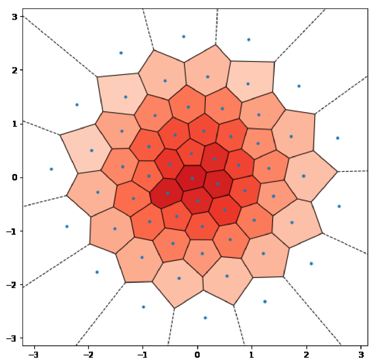
Figure 1: An optimal quantizer for $\mathcal{N}\big{(}\mathbf{0},\mathbf{I}_{2}\big{)}$
at level 60.

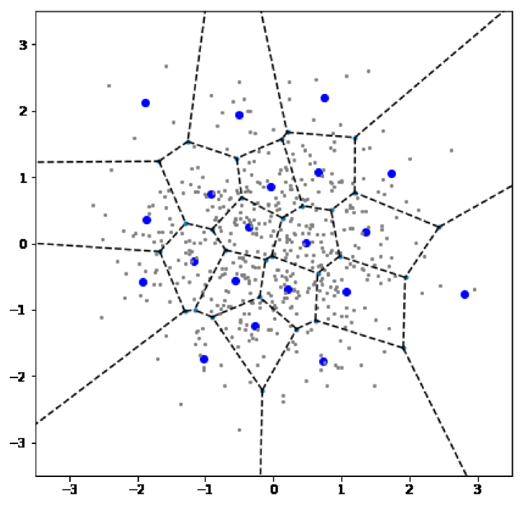
Figure 2: An optimal cluster center (blue points) for an observation $\{\eta_{1},...,\eta_{500}\}\mathrel{\overset{i.i.d}{\scalebox{1.5}[1.0]{$\sim$}}}\mathcal{N}(0,\mathbf{I}_{2})$ (grey points).

For $p\in[1,+\infty)$, let $\mathcal{P}_{p}(\mathbb{R}^{d})$ denote the set of all probability measures on $\mathbb{R}^{d}$ with a finite $p^{th}$-moment. Let $\mu,\nu\in\mathcal{P}_{p}(\mathbb{R}^{d})$ and let $\Pi(\mu,\nu)$ denote the set of all probability measures on $(\mathbb{R}^{d}\times\mathbb{R}^{d},Bor(\mathbb{R}^{d})^{\otimes 2})$ with marginals $\mu$ and $\nu$, where $Bor(\mathbb{R}^{d})$ denotes the Borel $\sigma$-algebra on $\mathbb{R}^{d}$. For $p\geq 1$, the $L^{p}$-Wasserstein distance $\mathcal{W}_{p}$ on $\mathcal{P}_{p}(\mathbb{R}^{d})$ is defined by

$$\mathcal{W}_{p}(\mu,\nu) =\Big{(}\inf_{\pi\in\Pi(\mu,\nu)}\int_{\mathbb{R}^{d}\times\mathbb{R}^{d}}\left|x-y\right|^{p}\pi(dx,dy)\Big{)}^{\frac{1}{p}}$$

$$=\inf\Big{\{}\Big{[}\mathbb{E}\;\left|X-Y\right|^{p}\Big{]}^{\frac{1}{p}},\;X,Y:(\Omega,\mathcal{A},\mathbb{P})\rightarrow(\mathbb{R}^{d},Bor(\mathbb{R}^{d}))\;\text{with}\;\mathbb{P}_{X}=\mu,\mathbb{P}_{Y}=\nu\;\Big{\}}.$$ (1.7)

The space $\mathcal{P}_{p}(\mathbb{R}^{d})$ equipped with the Wasserstein distance $\mathcal{W}_{p}$ is a Polish space, i.e. is separable and complete (see [Bol08]). If $\mu,\nu\in\mathcal{P}_{p}(\mathbb{R}^{d})$, then for any $q\leq p$, $\mathcal{W}_{q}(\mu,\nu)\leq\mathcal{W}_{p}(\mu,\nu).$

With a slight abuse of notation, we define the distortion function for the optimal quantization as follows.

Definition 1.1 (Distortion function).

Let $K\in\mathbb{N}^{*}$ be the quantization level. Let $\mu\in\mathcal{P}_{2}(\mathbb{R}^{d})$. The (quadratic) distortion function $\mathcal{D}_{K,\,\mu}$ of $\mu$ at level $K$ is defined by

$$x=(x_{1},...,x_{K})\in(\mathbb{R}^{d})^{K}\longmapsto\mathcal{D}_{K,\,\mu}(x)=\int_{\mathbb{R}^{d}}\min_{1\leq i\leq K}\left|\xi-x_{i}\right|^{2}\mu(d\xi)=e_{K,\mu}^{2}(x).$$ (1.8)

For a fixed (known) probability distribution $\mu$, its optimal quantizers can be computed by several algorithms such as the CLVQ algorithm (see e.g. [Pag15][Section 3.2]) or the Lloyd I algorithm (see e.g. [Llo82], [Kie82] and [PY16]). However, another situation exists: the probability distribution $\mu$ is unknown but there exists a known sequence $(\mu_{n})_{n\geq 1}$ converging in the Wasserstein distance to $\mu$. A typical example is the empirical measure of an i.i.d. $\mu$-distributed sequence random vectors (see (1.10) below). The empirical measure of non i.i.d. random vectors appears for example when dealing with the particle method associated to the McKean-Vlasov equations (see [Liu19][Section 7.1 and Section 7.5]) or the simulation of the invariant measure of the diffusion process (see [LP02] and [Lem05][Chapter 4]). This leads us to study the consistency and the convergence rate of the optimal quantization for a $\mathcal{W}_{p}$-converging probability distribution sequence $(\mu_{n})_{n\geq 1}$.

There exist several studies in the literature. The consistency of the optimal quantizers was first proved in [Pol82b].

Theorem (Pollard’s Theorem).

Let $\mu_{n}\in\mathcal{P}_{2}(\mathbb{R}^{d}),n\in\mathbb{N}^{*}\cup\{\infty\}$ with $\mathcal{W}_{2}(\mu_{n},\mu_{\infty})\rightarrow 0$ as $n\rightarrow+\infty$. Assume $\mathrm{card}\big{(}\mathrm{supp}(\mu_{n})\big{)}\geq K$, for $n\in\mathbb{N}^{*}\cup\{+\infty\}$. For $n\geq 1$, let $x^{(n)}=\big{(}x_{1}^{(n)},...,x_{K}^{(n)}\big{)}$ be a $K$-optimal quantizer for $\mu_{n}$, then the quantizer sequence $(x^{(n)})_{n\geq 1}$ is bounded in $\mathbb{R}^{d}$ and any limiting point of $(x^{(n)})_{n\geq 1}$, denoted by $x^{(\infty)}$, is an optimal quantizer of $\mu_{\infty}$.

Let $\mu_{n}\in\mathcal{P}_{2}(\mathbb{R}^{d}),\,n\in\mathbb{N}\cup\{\infty\}$ with $\mathcal{W}_{2}(\mu_{n},\mu_{\infty})\rightarrow 0$ as $n\rightarrow+\infty$. Let $x^{(n)}$ denote an optimal quantiser of $\mu_{n}$. There are two ways to study the convergence rate of the optimal quantizers. The first way is to directly evaluate the distance between $x^{(n)}$ and $\mathrm{argmin}\,\mathcal{D}_{K,\mu_{\infty}}$. The second way is called the quantization performance, defined by

$$\mathcal{D}_{K,\mu_{\infty}}(x^{(n)})-\inf_{x\in(\mathbb{R}^{d})^{K}}\mathcal{D}_{K,\mu_{\infty}}(x).$$ (1.9)

This quantity describes the distance between the optimal error of $\mu_{\infty}$ and the quantization error of $x^{(n)}$ considered as a quantizer of $\mu_{\infty}$ (even $x^{(n)}$ is obviously not “optimal” for $\mu_{\infty}$). Several results of convergence rate exist in the framework of the empirical measure. Let $X_{1}(\omega),...,X_{n}(\omega),...$ be i.i.d random vectors with probability distribution $\mu\in\mathcal{P}_{2}(\mathbb{R}^{d})$ and let

$$\mu^{\omega}_{n}\coloneqq\frac{1}{n}\sum_{i=1}^{n}\delta_{X_{i}(\omega)}$$ (1.10)

be the empirical measure of $\mu$. The almost sure convergence of $\mathcal{W}_{2}(\mu_{n}^{\omega},\mu)$ has been proved in [Pol82b][Theorem 7]. Let $x^{(n),\omega}$ denotes an optimal quantizer of $\mu_{n}^{\omega}$ at level $K$. In [Pol82a], the author has proved that if $\mu$ has a unique optimal quantizer $x$ at level $K$, then the convergence rate (convergence in distribution) of $\left|x^{(n),\omega}-x\right|$ is $\mathcal{O}(n^{-1/2})$ under appropriate conditions. Moreover, if $\mu$ has a support contained in $B(0,R)$, where $B(0,R)$ denotes the ball in $\mathbb{R}^{d}$ centered at $0$ with radius $R$, an upper bound of the mean performance has been proved in [BDL08], shown as follows,

$$\mathbb{E}\,\mathcal{D}_{K,\,\mu}(x^{(n),\omega})-\inf_{x\in(\mathbb{R}^{d})^{K}}\mathcal{D}_{K,\,\mu}(x)\leq\frac{12K\cdot R^{2}}{\sqrt{n}}.$$

In this paper, we extend the convergence results in [Pol82a] and in [BDL08] in two perspectives: first, we give an upper bound of the quantization performance

$$\mathcal{D}_{K,\mu_{\infty}}(x^{(n)})-\inf_{x\in(\mathbb{R}^{d})^{K}}\mathcal{D}_{K,\mu_{\infty}}(x).$$ (1.11)

and that of related optimal quantizers for any probability distribution sequence $(\mu_{n})_{n\geq 1}$ converging in the Wasserstein distance. Then, we generalize the clustering performance results in [BDL08] to empirical measures in $\mathcal{P}_{2}(\mathbb{R}^{d})$ possibly having an unbounded support.

Our main results are as follows. We obtain in Section 2 a non-asymptotic upper bound for the quantization performance: for every $n\in\mathbb{N}^{*}$,

$$\mathcal{D}_{K,\,\mu_{\infty}}(x^{(n)})-\inf_{x\in(\mathbb{R}^{d})^{K}}\mathcal{D}_{K,\,\mu_{\infty}}(x)\leq 4e_{K,\mu_{\infty}}^{*}\mathcal{W}_{2}(\mu_{n},\mu_{\infty})+4\mathcal{W}_{2}^{2}(\mu_{n},\mu_{\infty}).$$ (1.12)

Moreover, if $\mathcal{D}_{K,\mu_{\infty}}$ is twice differentiable at

$$F_{K}\coloneqq\big{\{}x=(x_{1},...,x_{K})\in(\mathbb{R}^{d})^{K}\;\big{|}\;x_{i}\neq x_{j},\text{ if }i\neq j\big{\}}$$ (1.13)

and if the Hessian matrix $H_{\mathcal{D}_{K,\mu_{\infty}}}$ of $\mathcal{D}_{K,\mu_{\infty}}$ is positive definite in the neighboorhood of every optimal quantizer $x^{(\infty)}\in G_{K}(\mu_{\infty})$ having the eigenvalues lower bounded by a $\lambda^{*}>0$, then, for $n$ large enough,

$$d\big{(}x^{(n)},G_{K}(\mu_{\infty})\big{)}^{2}\leq\frac{8}{\lambda^{*}}e_{K,\mu_{\infty}}^{*}\cdot\mathcal{W}_{2}(\mu_{n},\mu_{\infty})+\frac{8}{\lambda^{*}}\cdot\mathcal{W}^{2}_{2}(\mu_{n},\mu_{\infty}),$$

where $d(\xi,A)\coloneqq\min_{a\in A}\left|\xi-a\right|$ denotes the distance between a point $\xi\in\mathbb{R}^{d}$ and a set $A\subset\mathbb{R}^{d}$.

Several criterions for the positive definiteness of the Hessian matrix $H_{\mathcal{D}_{K,\mu}}$ of the distortion function $\mathcal{D}_{K,\mu}$ are established in Section 3. We show in Section 3.1 the conditions under which the distortion function $\mathcal{D}_{K,\mu}$ is twice differentiable in every $x\in F_{K}$ and give the exact formula of the Hessian matrix $H_{\mathcal{D}_{K,\mu}}$. Moreover, we also discuss several sufficient and necessary conditions for the positive definiteness of the Hessian matrix in dimension $d\geq 2$ and in dimension 1.

In Section 4, we give two upper bounds for the clustering performance $\mathbb{E}\,\mathcal{D}_{K,\,\mu}(x^{(n),\,\omega})-\inf_{x\in(\mathbb{R}^{d})^{K}}\mathcal{D}_{K,\,\mu}(x)$, where $x^{(n),\,\omega}$ is an optimal quantizer of $\mu_{n}^{\omega}$ defined in (1.10). If $\mu\in\mathcal{P}_{q}(\mathbb{R}^{d})$ for some $q>2$, a first upper bound is established in Proposition 4.1

$$\mathbb{E}\,\mathcal{D}_{K,\,\mu} (x^{(n),\omega})-\inf_{x\in(\mathbb{R}^{d})^{K}}\mathcal{D}_{K,\,\mu}(x)$$

$$\leq C_{d,q,\mu,K}\times\begin{cases}n^{-1/4}+n^{-(q-2)/2q}&\mathrm{if}\>d<4\>\mathrm{and}\>q\neq 4\\ n^{-1/4}\big{(}\log(1+n)\big{)}^{1/2}+n^{-(q-2)/2q}&\mathrm{if}\>d=4\>\mathrm{and}\>q\neq 4\\ n^{-1/d}+n^{-(q-2)/2q}&\mathrm{if}\>d>4\>\mathrm{and}\>q\neq d/(d-2)\end{cases},$$

where $C_{d,q,\mu,K}$ is a constant depending on $d,q,\mu$ and the quantization level $K$. This result is a direct application of the non-asymptotic upper bound (1.12) combined with results in [FG15] about the mean convergence rate of the empirical measure for the Wasserstein distance. If $d\geq 4$ and $q>\frac{2d}{d-2}$, this constant $C_{d,q,\mu,K}$ is roughly decreasing as $K^{-1/d}$ (see Remark 4.1). This upper bound is sharper in $K$ compared with the upper bound (1.14) below, although it suffers from the curse of dimensionality.

Meanwhile, we establish another upper bound for the clustering performance in Theorem 4.1, which is sharper in $n$ but increasing faster than linearly in $K$. This upper bound is

$$\mathbb{E}\,\mathcal{D}_{K,\,\mu}(x^{(n),\omega})-\inf_{x\in(\mathbb{R}^{d})^{K}}\mathcal{D}_{K,\,\mu}(x)\leq\frac{2K}{\sqrt{n}}\Big{[}r_{2n}^{2}+\rho_{K}(\mu)^{2}+2r_{1}\big{(}r_{2n}+\rho_{K}(\mu)\big{)}\Big{]},$$ (1.14)

where $r_{n}\coloneqq\big{\|}\max_{1\leq i\leq n}\left|X_{i}\right|\big{\|}_{2}$ and $\rho_{K}(\mu)$ is the maximum radius of optimal quantizers for $\mu$, defined by

$$\rho_{K}(\mu)\coloneqq\max\Big{\{}\max_{1\leq k\leq K}\left|x^{*}_{k}\right|,\;\;(x^{*}_{1},...,x^{*}_{K})\text{ is an optimal quantizer of $\mu$ at level $K$}\Big{\}}.$$ (1.15)

In particular, we give a precise upper bound for $\mu=\mathcal{N}(m,\Sigma)$, the multidimensionnal normal distribution

$$\mathbb{E}\,\mathcal{D}_{K,\,\mu}(x^{(n),\omega})-\inf_{x\in(\mathbb{R}^{d})^{K}}\mathcal{D}_{K,\,\mu}(x)\leq C_{\mu}\cdot\frac{2K}{\sqrt{n}}\Big{[}1+\log n+\gamma_{K}\log K\big{(}1+\frac{2}{d}\big{)}\Big{]},$$ (1.16)

where $\limsup_{K}\gamma_{K}=1$ and $C_{\mu}=12\cdot\Big{[}1\vee\log\big{(}2\int_{\mathbb{R}^{d}}\text{exp}(\frac{1}{4}\left|\xi\right|^{4})\mu(d\xi)\big{)}\Big{]}$. If $\mu=\mathcal{N}(0,\mathbf{I}_{d})$, $C_{\mu}=12(1+\frac{d}{2})\cdot\log 2$.

We start our discussion with a brief review on the properties of optimal quantization.

1.1 Properties of the Optimal Quantization

Let $G_{K}(\mu)=\mathrm{argmin}\,\mathcal{D}_{K,\mu}$ denote the set of all optimal quantizers at level $K$ of $\mu$ and let $e^{*}_{K,\mu}$ denote the optimal quantization error of $\mu$ defined in (1.5).

Proposition 1.1.

Let $K\in\mathbb{N}^{*}$. Let $\mu\in\mathcal{P}_{2}(\mathbb{R}^{d})$ and $\mathrm{card}\big{(}\mathrm{supp}(\mu)\big{)}\geq K$.

1. If $K\geq 2$, then $e_{K,\,\mu}^{*}<e_{K-1,\,\mu}^{*}$.

2. (Existence and boundedness of optimal quantizers) The set $G_{K}(\mu)$ is nonempty and compact so that $\rho_{K}(\mu)$ defined in (1.15) is finite for any fixed $K$. Moreover, if $x=(x_{1},...,x_{K})$ is an optimal quantizer of $\mu$, then $x\in F_{K}$, where $F_{K}$ is defined in (1.13).

3. If the support of $\mu$, denoted by $\mathrm{supp}(\mu)$, is a compact, then for every optimal quantizer $\,x=(x_{1},...,x_{K})\in G_{K}(\mu)$, its elements $x_{k},1\leq k\leq K$ are contained in the closure of convex hull of $\mathrm{supp}(\mu)$, denoted by $\mathcal{H}_{\mu}\coloneqq\overline{\mathrm{conv}\big{(}\mathrm{supp}(\mu)\big{)}}$.

For the proof of Proposition 1.1-(i) and (ii), we refer to [GL00][see Theorem 4.12] and for the proof of (iii) to Appendix B.

Theorem.

(Non-asymptotic Zador’s Theorem, see [LP08] and [Pag18][Theorem 5.2]) Let $\eta>0$. If $\mu\in\mathcal{P}_{2+\eta}(\mathbb{R}^{d})$, then for every quantization level $K$, there exists a constant $C_{d,\eta}\in(0,+\infty)$ which depends only on $d$ and $\eta$ such that

$$e_{K,\mu}^{*}\leq C_{d,\eta}\cdot\sigma_{2+\eta}(\mu)K^{-1/d},$$ (1.17)

where for $r\in(0,+\infty)$, $\sigma_{r}(\mu)=\min_{a\in\mathbb{R}^{d}}\big{[}\int_{\mathbb{R}^{d}}\left|\xi-a\right|^{r}\mu(d\xi)\big{]}^{1/r}$.

When $\mu$ has an unbounded support, we know from [PS12] that $\lim_{K}\rho_{K}(\mu)=+\infty$. The same paper also gives an asymptotic upper bound of $\rho_{K}$ when $\mu$ has a polynomial tail or a hyper-exponential tail.

Theorem.

([PS12][see Theorem 1.2]) Let $\mu\in\mathcal{P}_{p}(\mathbb{R}^{d})$ be absolutely continuous with respect to the Lebesgue measure $\lambda_{d}$ on $\mathbb{R}^{d}$ and let $f$ denote its density function.

1. Polynomial tail. For $p\geq 2$, if $\mu$ has a $c$-th polynomial tail with $c>d+p$ in the sense that there exists $\tau>0,\beta\in\mathbb{R}$ and $A>0$ such that $\forall\xi\in\mathbb{R}^{d},\left|\xi\right|\geq A\Longrightarrow\,f(\xi)=\frac{\tau}{\left|\xi\right|^{c}}(\log\left|\xi\right|)^{\beta}$, then

   $$\lim_{K}\frac{\log\rho_{K}}{\log K}=\frac{p+d}{d(c-p-d)}.$$ (1.18)

2. Hyper-exponential tail. If $\mu$ has a $(\vartheta,\kappa)$-hyper-exponential tail in the sense that there exists $\tau>0,\kappa,\vartheta>0,c>-d$ and $A>0$ such that $\forall\xi\in\mathbb{R}^{d},\left|\xi\right|\geq A\Longrightarrow\,f(\xi)=\tau\left|\xi\right|^{c}e^{-\vartheta\left|\xi\right|^{\kappa}}$, then

   $$\limsup_{K}\frac{\rho_{K}}{(\log K)^{1/\kappa}}\leq 2\vartheta^{-1/\kappa}\Big{(}1+\frac{2}{d}\Big{)}^{1/\kappa}.$$ (1.19)

   Furthermore, if $d=1$, $\lim_{K}\frac{\rho_{K}}{(\log K)^{1/\kappa}}=\big{(}\frac{3}{\vartheta}\big{)}^{1/\kappa}$.

We give now the definition of the radially controlled distribution, which will be useful to control the convergence rate of the density function $f(x)$ to 0 when $x$ converges in every direction to infinity.

Definition 1.2.

Let $\mu\in\mathcal{P}_{2}(\mathbb{R}^{d})$ be absolutely continuous with respect to the Lebesgue measure $\lambda_{d}$ on $\mathbb{R}^{d}$ having a continuous density function $f$. We call $\mu$ is $k$-radially controlled on $\mathbb{R}^{d}$ if there exists $A>0$ and a continuous non-increasing function $g:\mathbb{R}_{+}\rightarrow\mathbb{R}_{+}$ such that

$$\forall\xi\in\mathbb{R}^{d},\left|\xi\right|\geq A,\;\;\;\;\;\;\;\;\;f(\xi)\leq g(\left|\xi\right|)\;\text{and}\;\int_{\mathbb{R}_{+}}x^{d-1+k}g(x)dx<+\infty.$$

Note that the $c$-th polynomial tail with $c>k+d$ and the hyper-exponential tail are sufficient conditions to satisfy the $k$-radially controlled assumption. A typical example of hyper-exponential tail is the multidimensional normal distribution $\mathcal{N}(m,\Sigma)$.

For $\mu,\nu\in\mathcal{P}_{2}(\mathbb{R}^{d})$ and for every $K\in\mathbb{N}^{*}$, we have

$$\left\|e_{K,\mu}-e_{K,\nu}\right\|_{\sup}\coloneqq\sup_{x\in(\mathbb{R}^{d})^{K}}\left|e_{K,\,\mu}(x)-e_{K,\,\nu}(x)\right|\leq\mathcal{W}_{2}(\mu,\nu),$$ (1.20)

by a simple application of the triangle inequality for the $L^{2}-$norm (see e.g. [GL00] Formula (4.4) and Lemma 3.4). Hence, if $(\mu_{n})_{n\geq 1}$ is a sequence in $\mathcal{P}_{2}(\mathbb{R}^{d})$ converging for the $\mathcal{W}_{2}$-distance to $\mu_{\infty}\in\mathcal{P}_{2}(\mathbb{R}^{d})$, then for every $K\in\mathbb{N}^{*}$,

$$\left\|e_{K,\,\mu_{n}}-e_{K,\,\mu_{\infty}}\right\|_{\sup}\leq\mathcal{W}_{2}(\mu_{n},\mu_{\infty})\xrightarrow{n\rightarrow+\infty}0.$$ (1.21)

2 General Case

In this section, we first establish in Theorem 2.1 a non-asymptotic upper bound of the quantization performance $\mathcal{D}_{K,\,\mu_{\infty}}(x^{(n)})-\inf_{x\in(\mathbb{R}^{d})^{K}}\mathcal{D}_{K,\mu_{\infty}}(x)$. Then we discuss the convergence rate of the optimal quantizer sequence in Theorem 2.2.

Theorem 2.1 (Non-asymptotic upper bound for the quantization performance).

Let $K\in\mathbb{N}^{*}$ be the quantization level. For every $n\in\mathbb{N}^{*}\cup\{\infty\}$, let $\mu_{n}\in\mathcal{P}_{2}(\mathbb{R}^{d})$ with $\mathrm{card}\big{(}\mathrm{supp}(\mu_{n})\big{)}\geq K$. Assume that $\mathcal{W}_{2}(\mu_{n},\mu_{\infty})\rightarrow 0$ as $n\rightarrow+\infty$. For every $n\in\mathbb{N}^{*}$, let $x^{(n)}$ be an optimal quantizer of $\mu_{n}$. Then

$$\quad\mathcal{D}_{K,\mu_{\infty}}(x^{(n)})-\inf_{x\in(\mathbb{R}^{d})^{K}}\mathcal{D}_{K,\mu_{\infty}}(x)\leq 4e_{K,\mu_{\infty}}^{*}\mathcal{W}_{2}(\mu_{n},\mu_{\infty})+4\mathcal{W}_{2}^{2}(\mu_{n},\mu_{\infty}),$$

where $e_{K,\mu_{\infty}}^{*}$ is the optimal error of $\mu_{\infty}$ at level $K$ defined in (1.5).

Proof of Theorem 2.1.

Let $x^{(\infty)}$ be an optimal quantizer of $\mu_{\infty}$. Remark that here we do not need that $x^{(\infty)}$ is the limit of $x^{(n)}$. First, we have (see e.g. Corollary 4.1 in [Gyö02])

$$e_{K,\mu_{\infty}}(x^{(n)})-e_{K,\mu_{\infty}}^{*} =e_{K,\mu_{\infty}}(x^{(n)})-e_{K,\mu_{n}}(x^{(n)})+e_{K,\mu_{n}}(x^{(n)})-e_{K,\mu_{\infty}}(x^{(\infty)})$$

$$\leq 2\left\|e_{K,\mu_{\infty}}-e_{K,\mu_{n}}\right\|_{\sup}\leq 2\mathcal{W}_{2}(\mu_{n},\mu_{\infty}),$$ (2.1)

where the first inequality is due to the fact that for any $\mu,\nu\in\mathcal{P}_{2}(\mathbb{R}^{d})$ with respective $K$-level optimal quantizers $x^{\mu}$ and $x^{\nu}$, if $e_{K,\mu}(x^{\mu})\geq e_{K,\nu}(x^{\nu})$, we have

$$\left|e_{K,\mu}(x^{\mu})-e_{K,\nu}(x^{\nu})\right|=e_{K,\mu}(x^{\mu})-e_{K,\nu}(x^{\nu})\leq e_{K,\mu}(x^{\nu})-e_{K,\nu}(x^{\nu})\leq\left\|e_{K,\mu_{\infty}}-e_{K,\mu_{n}}\right\|_{\sup}.$$

If $e_{K,\mu}(x^{\mu})\leq e_{K,\nu}(x^{\nu})$, we have the same inequality by the same reasoning.

Moreover,

$$\mathcal{D}_{K,\mu_{\infty}}(x^{(n)}) -\inf_{x\in(\mathbb{R}^{d})^{K}}\mathcal{D}_{K,\mu_{\infty}}(x)=\mathcal{D}_{K,\mu_{\infty}}(x^{(n)})-\mathcal{D}_{K,\mu_{\infty}}(x^{(\infty)})$$

$$\leq\big{[}e_{K,\mu_{\infty}}(x^{(n)})+e_{K,\mu_{\infty}}(x^{(\infty)})\big{]}\big{(}e_{K,\mu_{\infty}}(x^{(n)})-e_{K,\mu_{\infty}}(x^{(\infty)})\big{)}$$

$$\leq 2\big{[}e_{K,\mu_{\infty}}(x^{(n)})-e_{K,\mu_{\infty}}(x^{(\infty)})+2e_{K,\mu_{\infty}}(x^{(\infty)})\big{]}\cdot\mathcal{W}_{2}(\mu_{n},\mu_{\infty})\quad\text{\big{(}by (\ref{perforerror})\big{)}}$$

$$\leq 4\big{[}\mathcal{W}_{2}(\mu_{n},\mu_{\infty})+e_{K,\mu_{\infty}}^{*}\big{]}\cdot\mathcal{W}_{2}(\mu_{n},\mu_{\infty})\quad\text{\big{(}by (\ref{perforerror})\big{)}}$$

$$\leq 4e_{K,\mu_{\infty}}^{*}\mathcal{W}_{2}(\mu_{n},\mu_{\infty})+4\mathcal{W}_{2}^{2}(\mu_{n},\mu_{\infty}).\hfill\qed$$

Let $B(x,r)$ denote the ball centered at $x$ with radius $r$. Recall that $F_{K}\coloneqq\big{\{}x=(x_{1},...,x_{K})\in(\mathbb{R}^{d})^{K}\;\big{|}\;x_{i}\neq x_{j},\text{ if }i\neq j\big{\}}$. Remark that if $x\in F_{K}$, then every $y\in B\big{(}x,\frac{1}{3}\min_{1\leq i,j\leq K,i\neq j}\left|x_{i}-x_{j}\right|\big{)}$ still lies in $F_{K}$. In the following theorem, we give an estimate of the convergence rate of the optimal quantizer sequence $x^{(n)},n\in\mathbb{N}^{*}$.

Theorem 2.2 (Convergence rate of optimal quantizers).

Let $K\in\mathbb{N}^{*}$ be the quantization level. For every $n\in\mathbb{N}^{*}\cup\{\infty\}$, let $\mu_{n}\in\mathcal{P}_{2}(\mathbb{R}^{d})$ with $\mathrm{card}\big{(}\mathrm{supp}(\mu_{n})\big{)}\geq K$. Assume that $\mathcal{W}_{2}(\mu_{n},\mu_{\infty})\rightarrow 0$ as $n\rightarrow+\infty$. For every $n\in\mathbb{N}^{*}$, let $x^{(n)}$ be an optimal quantizer of $\mu_{n}$ and let $G_{K}(\mu_{\infty})$ denote the set of all optimal quantizers of $\mu_{\infty}$. If the following assumptions hold

1. the distortion function $\mathcal{D}_{K,\mu_{\infty}}$ is twice differentiable at every $x\in F_{K}$;

2. $\mathrm{card}\big{(}G_{K}(\mu_{\infty})\big{)}<+\infty$;

3. for every $x^{(\infty)}\in G_{K}(\mu_{\infty})$, the Hessian matrix of $\mathcal{D}_{K,\mu_{\infty}}$, denoted by $H_{\mathcal{D}_{K,\mu_{\infty}}}$, is positive definite in the neighbourhood of $x^{(\infty)}$ having eigenvalues lower bounded by some $\lambda^{*}>0$,

then, for $n$ large enough,

$$d\big{(}x^{(n)},G_{K}(\mu_{\infty})\big{)}^{2}\leq\frac{8}{\lambda^{*}}e_{K,\mu_{\infty}}^{*}\cdot\mathcal{W}_{2}(\mu_{n},\mu_{\infty})+\frac{8}{\lambda^{*}}\cdot\mathcal{W}^{2}_{2}(\mu_{n},\mu_{\infty}).$$

Remark 2.1.

Section 3 provides a detailed discussion of the conditions in Theorem 2.2 and their relation between each other.

(1) First, in Section 3, we establish that if $\mu_{\infty}$ is $1$-radially controlled, then its distortion function $\mathcal{D}_{K,\mu_{\infty}}$ is twice continuously differentiable at every $x\in F_{K}$ and give an exact formula of the Hessian matrix $H_{\mathcal{D}_{K,\mu_{\infty}}}(x)$ in Proposition 3.1. Thus, one may obtain Condition $(c)$ either by an explicit computation or by numerical methods. Moreover, if $H_{\mathcal{D}_{K,\mu}}$ is positive definite at $x\in F_{K}$, it is also positive definite in its neighbourhood. In Section 3.2, we establish several sufficient conditions for the positive definiteness of the Hessian matrix $H_{\mathcal{D}_{K,\mu_{\infty}}}$ in the neighbourhood of $x^{(\infty)}\in G_{K}(\mu_{\infty})$ in one dimension.

(2) If the distribution $\mu_{\infty}$ is $1$-radially controlled, a necessary condition for Condition $(c)$ is Condition $(b)$ (see Lemma 3.1). Thus, if $\mathrm{card}\big{(}G_{K}(\mu_{\infty})\big{)}=+\infty$, it is more reasonable to consider the non-asymtotic upper bound of the performance (Theorem 2.1) to study the convergence rate of the optimal quantization. A typical example is the standard multidimensional normal distribution $\mu_{\infty}=\mathcal{N}(0,I_{d})$: it is $1$-radially controlled and any rotation of an optimal quantizer $x$ is still optimal so that $\mathrm{card}\big{(}G_{K}(\mu_{\infty})\big{)}=+\infty$.

Proof of Theorem 2.2.

Since the quantization level $K$ is fixed throughout the proof, we will drop the subscripts $K$ and $\mu$ of the distortion function $\mathcal{D}_{K,\,\mu}$ and we will denote by $\mathcal{D}_{n}$ (respectively, $\mathcal{D}_{\infty})$ the distortion function of $\mu_{n}$ (resp. $\mu_{\infty}$).

After Pollard’s theorem, $(x^{(n)})_{n\in\mathbb{N}^{*}}$ is bounded and any limiting point of $x^{(n)}$ lies in $G_{K}(\mu_{\infty})$. We may assume that, up to the extraction of a subsequence of $x^{(n)}$, still denoted by $x^{(n)}$, we have $x^{(n)}\rightarrow x^{(\infty)}\in G_{K}(\mu_{\infty})$. Hence $d\big{(}x^{(n)},G_{K}(\mu_{\infty})\big{)}\leq\left|x^{(n)}-x^{(\infty)}\right|$.

Proposition 1.1 implies that $x^{(\infty)}\in F_{K}$. As $\mathcal{D}_{\infty}$ is twice differentiable at $x^{(\infty)}$, the second order Taylor expansion of $\mathcal{D}_{\infty}$ at $x^{(\infty)}$ reads:

$$\mathcal{D}_{\infty}(x^{(n)})=\mathcal{D}_{\infty}(x^{(\infty)})+\big{\langle}\nabla\mathcal{D}_{\infty}(x^{(\infty)})\mid x^{(n)}-x^{(\infty)}\big{\rangle}+\frac{1}{2}H_{\mathcal{D}_{\infty}}(\zeta^{(n)})(x^{(n)}-x^{(\infty)})^{\otimes 2},$$

where $H_{\mathcal{D}_{\infty}}$ denotes the Hessian matrix of $\mathcal{D}_{\infty}$, $\zeta^{(n)}$ lies in the geometric segment $(x^{(n)},x^{(\infty)})$ and for a matrix $A$ and a vector $u$, $Au^{\otimes 2}$ stands for $u^{T}Au$.

As $x^{(\infty)}\in G_{K}(\mu_{\infty})=\text{argmin}\,\mathcal{D}_{\infty}$ and $\text{card}\big{(}\text{supp}(\mu_{\infty})\big{)}\geq K$, one has $\nabla\mathcal{D}_{\infty}(x^{(\infty)})=0$. Hence

$$\mathcal{D}_{\infty}(x^{(n)})-\mathcal{D}_{\infty}(x^{(\infty)})=\frac{1}{2}H_{\mathcal{D}_{\infty}}(\zeta^{(n)})(x^{(n)}-x^{(\infty)})^{\otimes 2}.$$ (2.2)

It follows from Theorem 2.1 that

$$H_{\mathcal{D}_{\infty}}(\zeta^{(n)})(x^{(n)}-x^{(\infty)})^{\otimes 2} =2\big{(}\mathcal{D}_{\infty}(x^{(n)})-\mathcal{D}_{\infty}(x^{(\infty)})\big{)}$$

$$\leq 8e_{K,\mu_{\infty}}^{*}\mathcal{W}_{2}(\mu_{n},\mu_{\infty})+8\mathcal{W}_{2}^{2}(\mu_{n},\mu_{\infty}).$$ (2.3)

By Condition (c), $H_{\mathcal{D}_{\infty}}$ is assumed to be positive definite in the neighbourhood of all $x^{(\infty)}\in G_{K}(\mu_{\infty})$ having eigenvalues lower bounded by some $\lambda^{*}>0$. As $\zeta^{(n)}$ lies in the geometric segment $(x^{(n)},x^{(\infty)})$ and $x^{(n)}\rightarrow x^{(\infty)}$, there exists an $n_{0}(x^{(\infty)})$ such that for all $n\geq n_{0}$, $H_{\mathcal{D}_{\infty}}(\zeta^{(n)})$ is a positive definite matrix. It follows that, for $n\geq n_{0}$,

$$\lambda^{*}\left|x^{(n)}-x^{(\infty)}\right|^{2} \leq H_{\mathcal{D}_{\infty}}(\zeta^{(n)})(x^{(n)}-x^{(\infty)})^{\otimes 2}$$

$$\leq 8e_{K,\mu_{\infty}}^{*}\mathcal{W}_{2}(\mu_{n},\mu_{\infty})+8\mathcal{W}_{2}^{2}(\mu_{n},\mu_{\infty}).$$

Thus, one can directly conclude by multiplying at each side of the above inequality by $\frac{1}{\lambda^{*}}$. ∎

Based on conditions in Theorem 2.2, if we know the exact limit of the optimal quantizer sequence $x^{(n)}$, we have the following result whose proof is similar to that of Theorem 2.2.

Corollary 2.1.

Let $K\in\mathbb{N}^{*}$ be the quantization level. For every $n\in\mathbb{N}^{*}\cup\{\infty\}$, let $\mu_{n}\in\mathcal{P}_{2}(\mathbb{R}^{d})$ with $\mathrm{card}\big{(}\mathrm{supp}(\mu_{n})\big{)}\geq K$. Assume that $\mathcal{W}_{2}(\mu_{n},\mu_{\infty})\rightarrow 0$ as $n\rightarrow+\infty$. Let $x^{(n)}\in\mathrm{argmin}\;\mathcal{D}_{K,\,\mu_{n}}$ such that $\lim_{n}x^{(n)}\rightarrow x^{(\infty)}$. If the Hessian matrix of $\mathcal{D}_{K,\,\mu_{\infty}}$ is positive definite in the neighbourhood of $x^{(\infty)}$, then, for $n$ large enough,

$$\left|x^{(n)}-x^{(\infty)}\right|^{2}\leq C^{(1)}_{\mu_{\infty}}\cdot\mathcal{W}_{2}(\mu_{n},\mu_{\infty})+C^{(2)}_{\mu_{\infty}}\cdot\mathcal{W}_{2}^{2}(\mu_{n},\mu_{\infty}),$$

where $C^{(1)}_{\mu_{\infty}}$ and $C^{(2)}_{\mu_{\infty}}$ are real constants only depending on $\mu_{\infty}$.

3 Hessian matrix $H_{\mathcal{D}_{K,\,\mu}}$ of the distortion function $\mathcal{D}_{K,\,\mu}$

Let $\mu\in\mathcal{P}_{2}(\mathbb{R}^{d})$ with $\mathrm{card}\big{(}\mathrm{supp}(\mu)\big{)}\geq K$ and let $x^{*}$ be an optimal quantizer of $\mu$ at level $K$. In Section 3.1, we show conditions under which the distortion function $\mathcal{D}_{K,\mu}$ is twice differentiable and give the exact formula of its Hessian matrix $H_{\mathcal{D}_{K,\,\mu}}$. In Section 3.2, we give several criterions for the positive definiteness of the Hessian matrix $H_{\mathcal{D}_{K,\,\mu}}$ in the neighbourhood of an optimal quantizer $x^{*}$ in dimension 1.

3.1 Hessian matrix $H_{\mathcal{D}_{K,\,\mu}}$ on $\mathbb{R}^{d}$

If $\mu$ is absolutely continuous with respect to the Lebesgue measure $\lambda_{d}$ on $\mathbb{R}^{d}$ with the density function $f$, then the distortion function $\mathcal{D}_{K,\,\mu}$ is differentiable (see [Pag98]) at all point $x=(x_{1},...,x_{K})\in F_{K}$ with

$$\frac{\partial\mathcal{D}_{K,\,\mu}}{\partial x_{i}}(x)=2\int_{V_{i}(x)}(x_{i}-\xi)f(\xi)\lambda_{d}(d\xi),\;\;\;\text{for}\;i=1,...,K.$$ (3.1)

In the following Proposition, we give a criterion for the twice differentiability of the distortion function $\mathcal{D}_{K,\mu}$.

Proposition 3.1.

Let $\mu\in\mathcal{P}_{2}(\mathbb{R}^{d})$ be absolutely continuous with respect to the Lebesgue measure $\lambda_{d}$ on $\mathbb{R}^{d}$ with a continuous density function $f$. If $\mu$ is $1$-radially controlled, then

1. the distortion function $\mathcal{D}_{K,\,\mu}$ is twice differentiable at every $x\in F_{K}$ and the Hessian matrix $H_{\mathcal{D}_{K,\mu}}(x)=\Big{[}\frac{\partial^{2}\mathcal{D}_{K,\,\mu}}{\partial x_{j}\partial x_{i}}(x)\Big{]}_{1\leq i\leq j\leq K}$ is defined by

   $$\frac{\partial^{2}\mathcal{D}_{K,\,\mu}}{\partial x_{j}\partial x_{i}}(x)=2\int_{V_{i}(x)\cap V_{j}(x)}(x_{i}-\xi)\otimes(x_{j}-\xi)\cdot\frac{1}{\left|x_{j}-x_{i}\right|}f(\xi)\lambda_{x}^{ij}(d\xi),\;\;\;\text{if $j\neq i$,}$$ (3.2)

   $$\frac{\partial^{2}\mathcal{D}_{K,\,\mu}}{\partial x_{i}^{2}}(x)=2\Big{[}\mu\big{(}V_{i}(x)\big{)}\mathrm{I}_{d}-\sum_{\begin{subarray}{c}i\neq j\\ 1\leq j\leq K\end{subarray}}\int_{V_{i}(x)\cap V_{j}(x)}(x_{i}-\xi)\otimes(x_{i}-\xi)\cdot\frac{1}{\left|x_{j}-x_{i}\right|}f(\xi)\lambda_{x}^{ij}(d\xi)\Big{]},$$ (3.3)

   where in (3.2) and (3.3), $u\otimes v\coloneqq[u^{i}v^{j}]_{1\leq i,j\leq d}$ for any two vectors $u=(u^{1},...,u^{d})$ and $v=(v^{1},...,v^{d})$ in $\mathbb{R}^{d}$;

2. every element $\frac{\partial^{2}\mathcal{D}_{K,\,\mu}}{\partial x_{j}\partial x_{i}}$ of the Hessian matrix $H_{\mathcal{D}_{K,\mu}}$ is continuous at every $x\in F_{K}$.

The proof of Proposition 3.1 is postponed to Appendix C. The following lemma shows that under the condition of Proposition 3.1, Condition (c) in Theorem 2.2 implies Condition (b).

Lemma 3.1.

Let $\mu\in\mathcal{P}_{2}(\mathbb{R}^{d})$ be absolutely continuous with the respect to the Lebesgue measure $\lambda_{d}$ on $\mathbb{R}^{d}$ with a continuous density function $f$. If $\mu_{\infty}$ is $1$-radially controlled and $\mathrm{card}\big{(}G_{K}(\mu_{\infty})\big{)}=+\infty$, then there exists a point $x\in G_{K}(\mu_{\infty})$ such that the Hessian matrix $H_{\mathcal{D}_{K,\mu_{\infty}}}$ of $\mathcal{D}_{K,\mu_{\infty}}$ at $x$ has an eigenvalue $0$.

Proof of Lemma 3.1.

We denote by $H_{\mathcal{D}_{\infty}}$ instead of $H_{\mathcal{D}_{K,\mu_{\infty}}}$ to simplify the notation. Proposition 1.1 implies that $G_{K}(\mu_{\infty})$ is a compact set. If $\mathrm{card}\big{(}G_{K}(\mu_{\infty})\big{)}=+\infty$, there exists $x,x^{(k)}\in G_{K}(\mu_{\infty}),k\in\mathbb{N}^{*}$ such that $x^{(k)}\rightarrow x$ when $k\rightarrow+\infty$. Set $u_{k}\coloneqq\frac{x^{(k)}-x}{\left|x^{(k)}-x\right|}$, $k\geq 1$, then we have $\left|u_{k}\right|=1$ for all $k\in\mathbb{N}^{*}$. Hence, there exists a subsequence $\varphi(k)$ of $k$ such that $u_{\varphi(k)}$ converges to some $\widetilde{u}$ with $\left|\widetilde{u}\right|=1$.

The Taylor expansion of $\mathcal{D}_{K,\mu_{\infty}}$ at $x$ reads:

$$\mathcal{D}_{K,\mu_{\infty}}(x^{\varphi(k)})=\mathcal{D}_{K,\mu_{\infty}}(x)+\big{\langle}\nabla\mathcal{D}_{K,\mu_{\infty}}(x)\;\big{|}\;x^{\varphi(k)}-x\big{\rangle}+\frac{1}{2}H_{\mathcal{D}_{\infty}}(\zeta^{\varphi(k)})(x^{\varphi(k)}-x)^{\otimes 2},$$

where $\zeta^{\varphi(k)}$ lies in the geometric segment $(x^{\varphi(k)},x)$. Since $x,x^{(k)},k\in\mathbb{N}^{*}\in G_{K}(\mu_{\infty})$, then $\nabla\mathcal{D}_{K,\mu_{\infty}}(x)=0$ and for any $k\in\mathbb{N}^{*}$, $\mathcal{D}_{K,\mu_{\infty}}(x^{\varphi(k)})=\mathcal{D}_{K,\mu_{\infty}}(x)$. Hence, for any $k\in\mathbb{N}^{*}$, $H_{\mathcal{D}_{\infty}}(\zeta^{\varphi(k)})(x^{\varphi(k)}-x)^{\otimes 2}=0$. Consequently, for any $k\in\mathbb{N}^{*}$,

$$H_{\mathcal{D}_{\infty}}(\zeta^{\varphi(k)})\Big{(}\frac{x^{\varphi(k)}-x}{\left|x^{\varphi(k)}-x\right|}\Big{)}^{\otimes 2}=0.$$

Thus we have $H_{\mathcal{D}_{\infty}}(x)\widetilde{u}^{\otimes 2}=0$ by letting $k\rightarrow+\infty$, so that $H_{\mathcal{D}_{\infty}}(x)$ has an eigenvalue $0$. ∎

3.2 A criterion for positive definiteness of $H_{\mathcal{D}_{\infty}}(x^{*})$ in 1-dimension

Let $\mu\in\mathcal{P}_{2}(\mathbb{R})$ with $\mathrm{card}\big{(}\mathrm{supp}(\mu)\big{)}\geq K$. Assume that $\mu$ is absolutely continuous with respect to the Lebesgue measure having a density function $f$. In the one-dimensional case, it is useful to point out a sufficient condition for the uniqueness of optimal quantizer. A probability distribution $\mu$ is called strongly unimodal if its density function $f$ satisfies that $I=\{f>0\}$ is an open (possibly unbounded) interval and $\log f$ is concave on $I$. Let $F_{K}^{+}:=\big{\{}x=(x_{1},...,x_{K})\in\mathbb{R}^{K}\mid-\infty<x_{1}<x_{2}<...<x_{K}<+\infty\big{\}}$.

Lemma 3.2.

For $K\in\mathbb{N}^{*}$, if $\mu$ is strongly unimodal with $\mathrm{card}\big{(}\mathrm{supp}(\mu)\big{)}\geq K$, then there is only one stationary (then optimal) quantizer of level $K$ in $F_{K}^{+}$.

We refer to [Kie83], [Tru82], [BP93] and [GL00][see Theorem 5.1] for the proof of Lemma 3.2 and for more details.

Given a $K$-tuple $x=(x_{1},...,x_{K})\in F_{K}^{+}$, the Voronoi region $V_{i}(x)$ can be explicitly written: $V_{1}(x)=(-\infty,\frac{x_{1}+x_{2}}{2}]$, $V_{K}(x)=[\frac{x_{K-1}+x_{K}}{2},+\infty)$ and $V_{i}(x)=[\frac{x_{i-1}+x_{i}}{2},\frac{x_{i}+x_{i+1}}{2}]$ for $i=2,...,K-1$. For all $x\in F_{K}^{+}$, $\mathcal{D}_{K,\,\mu}$ is differentiable at $x$ and by (3.1) and

$$\nabla\mathcal{D}_{K,\,\mu}(x)=\left[\int_{V_{i}(x)}2(x_{i}-\xi)f(\xi)d\xi\right]_{i=1,...,K}.$$ (3.4)

Therefore, as $\nabla\mathcal{D}_{K,\,\mu}(x^{*})=0$, one can solve the optimal quantizer $x^{*}\in F_{K}^{+}$ as follows,

$$x_{i}^{*}=\frac{\int_{V_{i}(x^{*})}\xi f(\xi)d\xi}{\mu\big{(}V_{i}(x^{*})\big{)}},\;\;\;\text{for}\;i=1,...,K.$$ (3.5)

For any $x\in F_{K}^{+}$, the Hessian matrix $H_{\mathcal{D}_{K,\mu}}$ of $\mathcal{D}_{K,\,\mu}$ at $x$ is a tridiagonal symmetry matrix and can be calculated as follows,

$$H_{\mathcal{D}_{K,\mu}}(x)=\left(\begin{array}[]{ccccccc}A_{1}-B_{1,2}&-B_{1,2}\\ &\ddots&\\ &-B_{i-1,i}&A_{i}-B_{i-1,i}-B_{i,i+1}&-B_{i,i+1}\\ &&&\ddots&\\ &&&&-B_{K-1,K}&A_{K}-B_{K-1,K}\end{array}\right),$$ (3.6)

where $A_{i}=2\mu\big{(}C_{i}(x)\big{)}$ for $1\leq i\leq K$ and $B_{i,j}=\frac{1}{2}(x_{j}-x_{i})f(\frac{x_{i}+x_{j}}{2})$ for $1\leq i<j\leq K$. Let $F_{\mu}$ be the cumulative distribution function of $\mu$, then

$$A_{1}=2\mu\big{(}C_{1}(x)\big{)}=2F_{\mu}\Big{(}\frac{x_{1}+x_{2}}{2}\Big{)},$$

$$A_{i}=2\mu\big{(}C_{i}(x)\big{)}=2\Big{[}F_{\mu}\Big{(}\frac{x_{i+1}+x_{i}}{2}\Big{)}-F_{\mu}\Big{(}\frac{x_{i-1}+x_{i}}{2}\Big{)}\Big{]},\quad\text{for }\,i=2,...,K-1,$$

$$A_{K}=2\mu\big{(}C_{K}(x)\big{)}=2\Big{[}1-F_{\mu}\Big{(}\frac{x_{K-1}+x_{K}}{2}\Big{)}\Big{]}.$$

Then the continuity of each term in the matrix $H_{\mathcal{D}_{K,\mu}}(x)$ can be directly derived from the continuity of $F_{\mu}$.

For $1\leq i\leq K$, we define $\displaystyle L_{i}(x)\coloneqq\sum_{j=1}^{K}\frac{\partial^{2}\mathcal{D}_{K,\,\mu}}{\partial x_{i}\partial x_{j}}(x)$. The following proposition gives sufficient conditions to obtain the positive definiteness of $H_{\mathcal{D}_{K,\mu}}(x^{*})$.

Proposition 3.2.

Let $\mu\in\mathcal{P}_{2}(\mathbb{R})$ with $\mathrm{card}\big{(}\mathrm{supp}(\mu)\big{)}\geq K$. Assume that $\mu$ is absolutely continuous with respect to the Lebesgue measure having a density function $f$. Any of the following two conditions implies the positive definiteness of $H_{\mathcal{D}_{K,\mu}}(x^{*})$,

1. $\mu$ is the uniform distribution,

2. $f$ is differentiable and $\log f$ is strictly concave.

In particular, $(ii)$ also implies that $L_{i}(x^{*})>0$, $i=1,...,K$.

Proposition 3.2 is proved in Appendix D. Remark that, under the conditions of Proposition 3.2, $\mu$ is strongly unimodal so that there is exactly one optimal quantizer in $F_{K}^{+}$ for $\mu$ at level $K$. The conditions in Proposition 3.2 directly imply the following convergence rate results.

Theorem 3.1.

Let $K\in\mathbb{N}^{*}$ be the quantization level. For every $n\in\mathbb{N}^{*}\cup\{\infty\}$, let $\mu_{n}\in\mathcal{P}_{2}(\mathbb{R})$ with $\mathrm{card}\big{(}\mathrm{supp}(\mu_{n})\big{)}\geq K$ be such that $\mathcal{W}_{2}(\mu_{n},\mu_{\infty})\rightarrow 0$ as $n\rightarrow+\infty$. Assume that $\mu_{\infty}$ is absolutely continuous with respect to the Lebesgue measure, written $\mu_{\infty}(d\xi)=f(\xi)d\xi$. Let $x^{(n)}$ be an optimal quantizer of $\mu_{n}$ converging to $x^{(\infty)}$. Then any one of the following two conditions

1. $\mu_{\infty}$ is the uniform distribution

2. $f$ is differentiable and $\log f$ is strictly concave

implies the existence of constants $C_{\mu_{\infty}}^{(1)}$ and $C_{\mu_{\infty}}^{(2)}$ only depending on $\mu_{\infty}$ such that for $n$ large enough,

$$\left|x^{(n)}-x^{(\infty)}\right|^{2}\leq C_{\mu_{\infty}}^{(1)}\cdot\mathcal{W}_{2}(\mu_{n},\mu_{\infty})+C_{\mu_{\infty}}^{(2)}\cdot\mathcal{W}_{2}^{2}(\mu_{n},\mu_{\infty}).$$

Proof.

Let $\mathcal{D}_{K,\,\mu_{\infty}}$ denote the distortion function of $\mu_{\infty}$ and let $H_{\mathcal{D}_{\infty}}$ denote the Hessian matrix of $\mathcal{D}_{K,\,\mu_{\infty}}$.

$(i)$ Let $g_{k}(x)$ be the $k$-th leading principal minor of $H_{\mathcal{D}_{\infty}}(x)$ defined in (3.6), then $g_{k}(x),k=1,...,K,$ are continuous functions in $x$ since every element in this matrix is continuous. Proposition 3.2 implies $g_{k}(x^{(\infty)})>0$, thus there exists $r>0$ such that for every $x\in B(x^{(\infty)},r)$, $g_{k}(x^{(\infty)})>0$ so that $H_{\mathcal{D}_{\infty}}(x)$ is positive definite. What remains can be directly proved by Corollary 2.1.

$(ii)$ The function $\displaystyle L_{i}(x)\coloneqq\sum_{j=1}^{K}\frac{\partial^{2}\mathcal{D}_{K,\,\mu_{\infty}}}{\partial x_{i}\partial x_{j}}(x)$ is continuous on $x$ and Proposition 3.2 implies that $L_{i}(x^{(\infty)})>0$. Hence, there exists $r>0$ such that $\forall x\in B(x^{(\infty)},r)$, $L_{i}(x)>0$. From (3.6), one can remark that the $i$-th diagonal elements in $H_{\mathcal{D}_{\infty}}(x)$ is always larger than $L_{i}(x)$ for any $x\in\mathbb{R}^{K}$, then after Gershgorin Circle theorem, we derive that $H_{\mathcal{D}_{\infty}}(x)$ is positive definite for every $x\in B(x^{(\infty)},r)$. What remains can be directly proved by Corollary 2.1. ∎

4 Empirical measure case

Let $K\in\mathbb{N}^{*}$ be the quantization level. Let $\mu\in\mathcal{P}_{2+\varepsilon}(\mathbb{R}^{d})$ for some $\varepsilon>0$ and $\mathrm{card}\big{(}\mathrm{supp}(\mu)\big{)}\geq K$. Let $X$ be a random variable with distribution $\mu$ and let $(X_{n})_{n\geq 1}$ be a sequence of independent identically distributed $\mathbb{R}^{d}$-valued random variables with probability distribution $\mu$. The empirical measure is defined for every $n\in\mathbb{N}^{*}$ by

$$\mu_{n}^{\omega}\coloneqq\frac{1}{n}\sum_{i=1}^{n}\delta_{X_{i}(\omega)},\;\;\;\omega\in\Omega,$$ (4.1)

where $\delta_{a}$ is the Dirac mass at $a$. For $n\geq 1$, let $x^{(n),\omega}$ be an optimal quantizer of $\mu_{n}^{\omega}$. The superscript $\omega$ is to emphasize that both $\mu_{n}^{\omega}$ and $x^{(n),\omega}$ are random and we will drop $\omega$ when there is no ambiguity. We cite two results of the convergence of $\mathcal{W}_{2}(\mu_{n}^{\omega},\mu)$ among so many researches in this topic: the a.s. convergence in [Pol82b][see Theorem 7] and the $L^{p}$-convergence rate of $\mathcal{W}_{p}(\mu_{n}^{\omega},\mu)$ in [FG15].

Theorem.

([FG15][see Theorem 1]) Let $p>0$ and let $\mu\in\mathcal{P}_{q}(\mathbb{R}^{d})$ for some $q>p$. Let $\mu_{n}^{\omega}$ denote the empirical measure of $\mu$ defined in (4.1). There exists a constant $C$ only depending on $p,d,q$ such that, for all $n\geq 1$,

$$\small{\mathbb{E}\Big{(}\mathcal{W}_{p}^{p}(\mu_{n}^{\omega},\mu)\Big{)}\leq CM_{q}^{p/q}(\mu)\times\begin{cases}n^{-1/2}+n^{-(q-p)/q}&\>\mathrm{if}\>p>d/2\>\mathrm{and}\>q\neq 2p\\ n^{-1/2}\log(1+n)+n^{-(q-p)/q}&\>\mathrm{if}\>p=d/2\>\mathrm{and}\>q\neq 2p\\ n^{-p/d}+n^{-(q-p)/q}&\>\mathrm{if}\>p\in(0,d/2)\>\mathrm{and}\>q\neq d/(d-p)\end{cases}},$$ (4.2)

where $M_{q}(\mu)=\int_{\mathbb{R}^{d}}\left|\xi\right|^{q}\mu(d\xi)$.

Let $\mathcal{D}_{K,\,\mu}$ denote the distortion function of $\mu$ and let $\mathcal{D}_{K,\,\mu_{n}}$ denote the distortion fuction of $\mu_{n}^{\omega}$ for any $n\in\mathbb{N}^{*}$. Recall by Definition 1.1 that for $c=(c_{1},...,c_{K})\in(\mathbb{R}^{d})^{K}$,

$$\mathcal{D}_{K,\,\mu}(c)=\mathbb{E}\min_{1\leq k\leq K}\left|X-c_{k}\right|^{2}=\mathbb{E}\Big{[}\left|X\right|^{2}+\min_{1\leq k\leq K}\big{(}-2\langle X|c_{k}\rangle+\left|c_{k}\right|^{2}\big{)}\Big{]},$$

$$\text{and}\;\;\mathcal{D}_{K,\,\mu_{n}}(c)=\frac{1}{n}\sum_{i=1}^{n}\min_{1\leq k\leq K}\left|X_{i}-c_{k}\right|^{2}=\frac{1}{n}\sum_{i=1}^{n}\left|X_{i}\right|^{2}+\min_{1\leq k\leq K}\left(-\frac{2}{n}\sum_{i=1}^{n}\langle X_{i}|c_{k}\rangle+\left|c_{k}\right|^{2}\right).$$

The a.s. convergence of optimal quantizers for the empirical measure has been proved in [Pol81]. We give a first upper bound of the clustering performance by applying directly Theorem 2.1 and (4.2).

Proposition 4.1.

Let $K\in\mathbb{N}^{*}$ be the quantization level. Let $\mu\in\mathcal{P}_{q}(\mathbb{R}^{d})$ for some $q>2$ with $\text{card}(\text{supp}(\mu))\geq K$ and let $\mu_{n}^{\omega}$ be the empirical measure of $\mu$ defined in (4.1). Let $x^{(n),\omega}$ be an optimal quantizer at level $K$ of $\mu_{n}^{\omega}$. Then for any $n>K$,

$$\mathbb{E}\,\mathcal{D}_{K,\,\mu} (x^{(n),\omega})-\inf_{x\in(\mathbb{R}^{d})^{K}}\mathcal{D}_{K,\,\mu}(x)$$

$$\leq C_{d,q,\mu,K}\times\begin{cases}n^{-1/4}+n^{-(q-2)/2q}&\mathrm{if}\>d<4\>\mathrm{and}\>q\neq 4\\ n^{-1/4}\big{(}\log(1+n)\big{)}^{1/2}+n^{-(q-2)/2q}&\mathrm{if}\>d=4\>\mathrm{and}\>q\neq 4\\ n^{-1/d}+n^{-(q-2)/2q}&\mathrm{if}\>d>4\>\mathrm{and}\>q\neq d/(d-2)\end{cases}.$$ (4.3)

where $C_{d,q,\mu,K}$ is a constant depending on $d,q,\mu$ and the quantization level $K$.

The reason why we only consider $n>K$ is that for a fixed $n\in\mathbb{N}^{*}$, the empirical measure $\mu_{n}$ defined in (4.1) is supported by $n$ points, which implies that, if $n\leq K$, the optimal quantizer of $\mu_{n}$ at level $K$, viewed as a set, is in fact $\mathrm{supp}(\mu_{n})$. This makes the above bound of no interest. Following the remark after Theorem 1 in [FG15], one can remark that if the probability distribution $\mu$ has sufficiently large moments (namely if $q>4$ when $d\leq 4$ and $q>2d/(d-2)$ when $d>4$), then the term $n^{-(q-2)/2q}$ is negligible and can be removed.

Proof of Proposition 4.1.

For every $\omega\in\Omega$ and for every $n>K$, Theorem 2.1 implies that

$$\mathcal{D}_{K,\mu}(x^{(n),\omega})-\inf_{x\in(\mathbb{R}^{d})^{K}}\mathcal{D}_{K,\mu}(x)\leq 4e_{K,\mu}^{*}\mathcal{W}_{2}(\mu_{n}^{\omega},\mu)+4\mathcal{W}_{2}^{2}(\mu_{n}^{\omega},\mu).$$

Thus,

$$\mathbb{E}\,\mathcal{D}_{K,\mu}(x^{(n),\omega})-\inf_{x\in(\mathbb{R}^{d})^{K}}\mathcal{D}_{K,\mu}(x)\leq 4e_{K,\mu}^{*}\mathbb{E}\,\mathcal{W}_{2}(\mu_{n}^{\omega},\mu)+4\,\mathbb{E}\,\mathcal{W}_{2}^{2}(\mu_{n}^{\omega},\mu).$$

It follows from (4.2) applied with $p=2$ that

$$\mathbb{E}\,\mathcal{W}_{2}^{2}(\mu_{n}^{\omega},\mu) \leq C_{d,q,\mu}\times\begin{cases}n^{-1/2}+n^{-(q-2)/q}&\mathrm{if}\>d<4\>\mathrm{and}\>q\neq 4\\ n^{-1/2}\log(1+n)+n^{-(q-2)/q}&\mathrm{if}\>d=4\>\mathrm{and}\>q\neq 4\\ n^{-2/d}+n^{-(q-2)/q}&\mathrm{if}\>d>4\>\mathrm{and}\>q\neq d/(d-2)\end{cases},$$ (4.4)

where $C_{d,q,\mu}=C\cdot M_{q}^{2/q}(\mu)$ and $C$ is the constant in $(\ref{nico})$. Moreover, as $\mathbb{E}\,\mathcal{W}_{2}(\mu_{n}^{\omega},\mu)\leq\big{(}\mathbb{E}\mathcal{W}_{2}^{2}(\mu_{n}^{\omega},\mu)\big{)}^{1/2}$ and $\sqrt{a+b}\leq\sqrt{a}+\sqrt{b}$ for any $a,b\in\mathbb{R}_{+}$, Inequality (4.2) also implies

$$\mathbb{E}\,\mathcal{W}_{2}(\mu_{n}^{\omega},\mu) \leq C_{d,q,\mu}^{1/2}\times\begin{cases}n^{-1/4}+n^{-(q-2)/2q}&\mathrm{if}\>d<4\>\mathrm{and}\>q\neq 4\\ n^{-1/4}\big{(}\log(1+n)\big{)}^{1/2}+n^{-(q-2)/2q}&\mathrm{if}\>d=4\>\mathrm{and}\>q\neq 4\\ n^{-1/d}+n^{-(q-2)/2q}&\mathrm{if}\>d>4\>\mathrm{and}\>q\neq d/(d-2)\end{cases}.$$

Consequently,

$$\mathbb{E}\,\mathcal{D}_{K,\mu}(x^{(n),\omega}) -\inf_{x\in(\mathbb{R}^{d})^{K}}\mathcal{D}_{K,\mu}(x)\leq 4e_{K,\mu}^{*}\mathbb{E}\,\mathcal{W}_{2}(\mu_{n}^{\omega},\mu)+4\,\mathbb{E}\,\mathcal{W}_{2}^{2}(\mu_{n}^{\omega},\mu).$$

$$\leq 8(C_{d,q,\mu}^{1/2}e_{K,\mu}^{*}\vee C_{d,q,\mu})\times$$

$$\;\;\;\;\begin{cases}n^{-1/4}+n^{-(q-2)/2q}&\mathrm{if}\>d<4\>\mathrm{and}\>q\neq 4\\ n^{-1/4}\big{(}\log(1+n)\big{)}^{1/2}+n^{-(q-2)/2q}&\mathrm{if}\>d=4\>\mathrm{and}\>q\neq 4\\ n^{-1/d}+n^{-(q-2)/2q}&\mathrm{if}\>d>4\>\mathrm{and}\>q\neq d/(d-2)\end{cases}.$$ (4.5)

One can conclude by setting $C_{d,q,\mu,K}\coloneqq 8(C_{d,q,\mu}^{1/2}e_{K,\mu}^{*}\vee C_{d,q,\mu})$. ∎

Remark 4.1.

When $d\geq 4$, if $\frac{q-2}{q}>\frac{2}{d}$ i.e. $q>\frac{2d}{d-2}$, Inequality (4.4) can be upper bounded as follows,

$$\mathbb{E}\,\mathcal{W}_{2}^{2}(\mu_{n}^{\omega},\mu)\leq 2C_{d,q,\mu}n^{-1/d}\times\begin{cases}n^{-\frac{1}{4}}\log(1+n)&\mathrm{if}\>d=4\>\mathrm{and}\>q\neq 4\\ n^{-\frac{1}{d}}&\mathrm{if}\>d>4\>\mathrm{and}\>q\neq d/(d-2)\end{cases}$$

$$\leq 2C_{d,q,\mu}K^{-1/d}\times\begin{cases}n^{-\frac{1}{4}}\log(1+n)&\mathrm{if}\>d=4\>\mathrm{and}\>q\neq 4\\ n^{-\frac{1}{d}}&\mathrm{if}\>d>4\>\mathrm{and}\>q\neq d/(d-2)\end{cases},$$

since we consider only $n\geq K$ and if $q>\frac{2d}{d-2}$, the term $n^{-(q-2)/2q}$ becomes negligible as $n$ grows. Consequently, (4) can be bounded by

$$\mathbb{E}\, \mathcal{D}_{K,\mu}(x^{(n),\omega})-\inf_{x\in(\mathbb{R}^{d})^{K}}\mathcal{D}_{K,\mu}(x)\leq 4e_{K,\mu}^{*}\mathbb{E}\,\mathcal{W}_{2}(\mu_{n}^{\omega},\mu)+4\,\mathbb{E}\,\mathcal{W}_{2}^{2}(\mu_{n}^{\omega},\mu).$$

$$\leq 8(C_{d,q,\mu}^{1/2}e_{K,\mu}^{*}\vee 2C_{d,q,\mu}K^{-1/d})\times$$

$$\;\;\;\begin{cases}n^{-\frac{1}{4}}\big{[}(\log(1+n))^{\frac{1}{2}}+\log(1+n)\big{]}&\mathrm{if}\>d=4\>\mathrm{and}\>q\neq 4\\ 2n^{-\frac{1}{d}}&\mathrm{if}\>d>4\>\mathrm{and}\>q\neq d/(d-2)\end{cases}.$$ (4.6)

By the non-asymptotic Zador theorem (1.17), one has

$$e_{K,\mu}^{*}\leq C_{d,q}(\mu)\sigma_{q}(\mu)K^{-1/d}$$

with $\sigma_{q}(\mu)=\min_{a\in\mathbb{R}^{d}}\left[\int_{\mathbb{R}^{d}}\left|\xi-a\right|^{q}\mu(d\xi)\right]^{1/q}$. Thus, Inequality (4.1) can be upper-bounded as follows,

$$\mathbb{E}\, \mathcal{D}_{K,\mu}(x^{(n),\omega})-\inf_{x\in(\mathbb{R}^{d})^{K}}\mathcal{D}_{K,\mu}(x)\leq 4e_{K,\mu}^{*}\mathbb{E}\,\mathcal{W}_{2}(\mu_{n}^{\omega},\mu)+4\,\mathbb{E}\,\mathcal{W}_{2}^{2}(\mu_{n}^{\omega},\mu).$$

$$\leq 8K^{-1/d}\big{(}C_{d,q,\mu}^{1/2}C_{d,q}(\mu)\sigma_{q}(\mu)\vee 2C_{d,q,\mu}\big{)}\times$$

$$\;\;\;\begin{cases}n^{-\frac{1}{4}}\big{[}(\log(1+n))^{\frac{1}{2}}+\log(1+n)\big{]}&\mathrm{if}\>d=4\>\mathrm{and}\>q\neq 4\\ 2n^{-\frac{1}{d}}&\mathrm{if}\>d>4\>\mathrm{and}\>q\neq d/(d-2)\end{cases},$$

from which one can remark that the constant $C_{d,q,\mu,K}$ in Proposition 4.1 is roughly decreasing as $K^{-1/d}$.

A second upper bound of the clustering performance is provided in the following theorem.

Theorem 4.1.

Let $K\in\mathbb{N}^{*}$ be the quantization level. Let $\mu\in\mathcal{P}_{2}(\mathbb{R}^{d})$ with $\text{card}\,(\text{supp}(\mu))\geq K$ and let $\mu_{n}^{\omega}$ be the empirical measures of $\mu$ defined in (4.1), generated by i.i.d observations $X_{1},...,X_{n},...$. We denote by $x^{(n),\omega}\in(\mathbb{R}^{d})^{K}$ an optimal quantizer of $\mu_{n}^{\omega}$ at level $K$. Then,

1. General upper bound of the performance.

   $$\mathbb{E}\,\mathcal{D}_{K,\,\mu}(x^{(n),\omega})-\inf_{x\in(\mathbb{R}^{d})^{K}}\mathcal{D}_{K,\,\mu}(x)\leq\frac{2K}{\sqrt{n}}\Big{[}r_{2n}^{2}+\rho_{K}(\mu)^{2}+2r_{1}\big{(}r_{2n}+\rho_{K}(\mu)\big{)}\Big{]},$$ (4.7)

   where $r_{n}\coloneqq\big{\|}\max_{1\leq i\leq n}\left|X_{i}\right|\big{\|}_{2}$ and $\rho_{K}(\mu)$ is the maximum radius of optimal quantizers of $\mu$, defined in (1.15).

2. Asymptotic upper bound for distribution with polynomial tail. For $p>2$, if $\mu$ has a $c$-th polynomial tail with $c>d+p$, then

   $$\mathbb{E}\,\mathcal{D}_{K,\,\mu}(x^{(n),\omega})-\inf_{x\in(\mathbb{R}^{d})^{K}}\mathcal{D}_{K,\,\mu}(x)\leq\frac{K}{\sqrt{n}}\Big{[}C_{\mu,p}\,n^{2/p}+6K^{\frac{2(p+d)}{d(c-p-d)}\gamma_{K}}\Big{]},$$

   where $C_{\mu,p}$ is a constant depending $\mu,p$ and $\lim_{K}\gamma_{K}=1$.

3. Asymptotic upper bound for distribution with hyper-exponential tail. Recall that $\mu$ has a hyper-exponential tail if $\mu=f\cdot\lambda_{d}$ and there exists $\tau>0,\kappa,\vartheta>0,c>-d$ and $A>0$ such that $\forall\xi\in\mathbb{R}^{d},\left|\xi\right|\geq A\Rightarrow\,f(\xi)=\tau\left|\xi\right|^{c}e^{-\vartheta\left|\xi\right|^{\kappa}}$. If $\kappa\geq 2$, we can obtain a more precise upper bound of the performance

   $$\mathbb{E}\big{[}\mathcal{D}_{K,\,\mu}(x^{(n),\omega})-\inf_{x\in(\mathbb{R}^{d})^{K}}\mathcal{D}_{K,\,\mu}(x)\big{]}\leq C_{\vartheta,\kappa,\mu}\cdot\frac{K}{\sqrt{n}}\Big{[}1+(\log n)^{2/\kappa}+\gamma_{K}(\log K)^{2/\kappa}\big{(}1+\frac{2}{d}\big{)}^{2/\kappa}\Big{]},$$

   where $C_{\vartheta,\kappa,\mu}$ is a constant depending $\vartheta,\kappa,\mu$ and $\limsup_{K}\gamma_{K}=1$.
   In particular, if $\mu=\mathcal{N}(m,\Sigma)$, the multidimensional normal distribution, we have

   $$\mathbb{E}\big{[}\mathcal{D}_{K,\,\mu}(x^{(n),\omega})-\inf_{x\in(\mathbb{R}^{d})^{K}}\mathcal{D}_{K,\,\mu}(x)\big{]}\leq C_{\mu}\cdot\frac{K}{\sqrt{n}}\Big{[}1+\log n+\gamma_{K}\cdot(\log K)\big{(}1+\frac{2}{d}\big{)}\Big{]},$$

   where $\limsup_{K}\gamma_{K}=1$ and $C_{\mu}=24\cdot\big{(}1\vee\log 2\mathbb{E}e^{\left|X\right|^{2}/4}\big{)}$ where $X$ is a random variable with distribution $\mu$. Moreover, when $\mu=\mathcal{N}(0,\mathbf{I}_{d})$, $C_{\mu}=24(1+\frac{d}{2})\cdot\log 2$.

The proof of Theorem 4.1 relies on the Rademacher process theory. A Rademacher sequence $(\sigma_{i})_{i\in\{1,...,n\}}$ is a sequence of i.i.d random variables with a symmetric $\{\pm 1\}$-valued Bernoulli distribution, independent of $(X_{1},...,X_{n})$ and we define the Rademacher process $\mathcal{R}_{n}(f),f\in\mathcal{F}$ by $\mathcal{R}_{n}(f)\coloneqq\frac{1}{n}\sum_{i=1}^{n}\sigma_{i}f(X_{i})$. Remark that the Rademacher process $\mathcal{R}_{n}(f)$ depends on the sample $\{X_{1},...,X_{n}\}$ of the probability measure $\mu$.

Theorem (Symmetrization inequalites).

For any class $\mathcal{F}$ of $\mu$-integrable functions, we have

$$\mathbb{E}\left\|\mu_{n}-\mu\right\|_{\mathcal{F}}\leq 2\mathbb{E}\left\|\mathcal{R}_{n}\right\|_{\mathcal{F}},$$

where for a probability distribution $\nu$, $\left\|\nu\right\|_{\mathcal{F}}\coloneqq\sup_{f\in\mathcal{F}}\left|\nu(f)\right|\coloneqq\sup_{f\in\mathcal{F}}\left|\int_{\mathbb{R}^{d}}fd\nu\right|$ and $\left\|\mathcal{R}_{n}\right\|_{\mathcal{F}}\coloneqq\sup_{f\in\mathcal{F}}\left|\mathcal{R}_{n}(f)\right|$.

For the proof of the above theorem, we refer to [Kol11][see Theorem 2.1]. Another more detailed reference is [VDVW96][see Lemma 2.3.1]. We will also introduce the Contraction principle in the following theorem and we refer to [BLM13][see Theorem 11.6] for the proof.

Theorem (Contraction principle).

Let $x_{1},...,x_{n}$ be vectors whose real-valued components are indexed by $\mathcal{T}$, that is, $x_{i}=(x_{i,s})_{s\in\mathcal{T}}$. For each $i=1,...,n$, let $\varphi_{i}:\mathbb{R}\rightarrow\mathbb{R}$ be a Lipschitz function such that $\varphi_{i}(0)=0$. Let $\sigma_{1},...,\sigma_{n}$ be independent Rademacher random variables and let $c_{L}=\max_{1\leq i\leq n}\sup_{\begin{subarray}{c}x,y\in\mathbb{R}\\ x\neq y\end{subarray}}\left|\frac{\varphi_{i}(x)-\varphi_{i}(y)}{x-y}\right|$ be the uniform Lipschitz constant of the function $\varphi_{i}$. Then

$$\mathbb{E}\Big{[}\sup_{s\in\mathcal{T}}\sum_{i=1}^{n}\sigma_{i}\varphi_{i}(x_{i,s})\Big{]}\leq c_{L}\cdot\mathbb{E}\Big{[}\sup_{s\in\mathcal{T}}\sum_{i=1}^{n}\sigma_{i}x_{i,s}\Big{]}.$$ (4.8)

Remark that, if we consider random variables $(Y_{1,s},...,Y_{n,s})_{s\in\mathcal{T}}$ independent of $(\sigma_{1},...,\sigma_{n})$ and for all $s\in\mathcal{T}$ and $i\in\{1,...,n\}$, $Y_{i,s}$ is valued in $\mathbb{R}$, then (4.8) implies that

$$\mathbb{E}\Big{[}\sup_{s\in\mathcal{T}}\sum_{i=1}^{n} \sigma_{i}\varphi_{i}(Y_{i,s})\Big{]}=\mathbb{E}\Big{\{}\mathbb{E}\Big{[}\sup_{s\in\mathcal{T}}\sum_{i=1}^{n}\sigma_{i}\varphi_{i}(Y_{i,s})\mid(Y_{1,s},...,Y_{n,s})_{s\in\mathcal{T}}\Big{]}\Big{\}}$$

$$\leq c_{L}\cdot\mathbb{E}\Big{\{}\mathbb{E}\Big{[}\sup_{s\in\mathcal{T}}\sum_{i=1}^{n}\sigma_{i}Y_{i,s}\mid(Y_{1,s},...,Y_{n,s})_{s\in\mathcal{T}}\Big{]}\Big{\}}\leq c_{L}\cdot\mathbb{E}\Big{[}\sup_{s\in\mathcal{T}}\sum_{i=1}^{n}\sigma_{i}Y_{i,s}\big{]}.$$ (4.9)

The proof of Theorem 4.1 is inspired by that of Theorem 2.1 in [BDL08].

Proof of Theorem 4.1.

(a) In order to simplify the notation, we will denote by $\mathcal{D}$ (respectively $\mathcal{D}_{n}$) instead of $\mathcal{D}_{K,\,\mu}$ (resp. $\mathcal{D}_{K,\,\mu_{n}}$) the distortion function of $\mu$ (resp. $\mu_{n}$). For any $c=(c_{1},...,c_{K})\in(\mathbb{R}^{d})^{K}$, note that the distortion function $\mathcal{D}(c)$ of $\mu$ can be written as

$$\mathcal{D}(c)=\mathbb{E}\big{[}\min_{1\leq k\leq K}\left|X-c_{k}\right|^{2}\big{]}=\mathbb{E}\big{[}\left|X\right|^{2}+\min_{1\leq k\leq K}(-2\langle X|c_{k}\rangle+\left|c_{k}\right|^{2})\big{]}.$$

We define $\overline{\mathcal{D}}(c)\coloneqq\min_{1\leq k\leq K}\big{(}-2\langle X|c_{k}\rangle+\left|c_{k}\right|^{2}\big{)}$. Similarly, for the distortion function $\mathcal{D}_{n}$ of the empirical measure $\mu_{n}$,

$$\mathcal{D}_{n}(c)=\frac{1}{n}\sum_{i=1}^{n}\min_{1\leq k\leq K}\left|X_{i}-c_{k}\right|^{2}=\frac{1}{n}\sum_{i=1}^{n}\left|X_{i}\right|^{2}+\min_{1\leq k\leq K}\big{(}-\frac{2}{n}\sum_{i=1}^{n}\langle X_{i}|c_{k}\rangle+\left|c_{k}\right|^{2}\big{)},$$

we define $\overline{\mathcal{D}}_{n}(c)\coloneqq\min_{1\leq k\leq K}\big{(}-\frac{2}{n}\sum_{i=1}^{n}\langle X_{i}|c_{k}\rangle+\left|c_{k}\right|^{2}\big{)}$. We will drop $\omega$ in $x^{(n),\omega}$ to alleviate the notation throughout the proof. Let $x\in\mathrm{argmin}\,\mathcal{D}_{K,\mu}$. It follows that

$$\mathbb{E}\big{[}\mathcal{D}(x^{(n)})-\mathcal{D}(x)\big{]} =\mathbb{E}\big{[}\overline{\mathcal{D}}(x^{(n)})-\overline{\mathcal{D}}(x)\big{]}=\mathbb{E}\big{[}\overline{\mathcal{D}}(x^{(n)})-\overline{\mathcal{D}}_{n}(x^{(n)})\big{]}+\mathbb{E}\big{[}\overline{\mathcal{D}}_{n}(x^{(n)})-\overline{\mathcal{D}}(x)\big{]}$$

$$\leq\mathbb{E}\big{[}\overline{\mathcal{D}}(x^{(n)})-\overline{\mathcal{D}}_{n}(x^{(n)})\big{]}+\mathbb{E}\big{[}\overline{\mathcal{D}}_{n}(x)-\overline{\mathcal{D}}(x)\big{]}.$$ (4.10)

Define for $\eta,x\in\mathbb{R}^{d}$, $f_{\eta}(x)=-2\langle\eta|x\rangle+\left|\eta\right|^{2}$.

Part (i): Upper bound of $\mathbb{E}[\overline{\mathcal{D}}(x^{(n)})-\overline{\mathcal{D}}_{n}(x^{(n)})]$. Let $R_{n}(\omega)\coloneqq\max_{1\leq i\leq n}\left|X_{i}(\omega)\right|$. Remark that for every $\omega\in\Omega$, $R_{n}(\omega)$ is invariant with the respect to all permutations of the components of $(X_{1},...,X_{n})$. Let $B_{R}$ denote the ball centred at 0 with radius $R$. Then, owing to Proposition 1.1-(iii), $x^{(n)}=(x^{(n)}_{1},...,x^{(n)}_{K})\in B_{R_{n}}^{K}$. Hence,

$$\mathbb{E}\,[\overline{\mathcal{D}}(x^{(n)})- \overline{\mathcal{D}}_{n}(x^{(n)})]\leq\mathbb{E}\,\sup_{c\,\in B_{R_{n}}^{K}}\big{(}\overline{\mathcal{D}}(c)-\overline{\mathcal{D}}_{n}(c)\big{)}$$

$$= \;\mathbb{E}\,\big{[}\sup_{c\,\in B_{R_{n}}^{K}}\big{(}\mathbb{E}\min_{1\leq k\leq K}f_{c_{k}}(X)-\frac{1}{n}\sum_{i=1}^{n}\min_{1\leq k\leq K}f_{c_{k}}(X_{i})\big{)}\big{]}$$

$$= \;\mathbb{E}\,\Big{[}\sup_{c\,\in B_{R_{n}}^{K}}\mathbb{E}\big{[}\frac{1}{n}\sum_{i=1}^{n}\min_{1\leq k\leq K}f_{c_{k}}(X^{\prime}_{i})-\frac{1}{n}\sum_{i=1}^{n}\min_{1\leq k\leq K}f_{c_{k}}(X_{i})\big{|}X_{1},...,X_{n}\big{]}\Big{]},$$ (4.11)

where $X^{\prime}_{1},...,X^{\prime}_{n}$ are i.i.d random variable with the distribution $\mu$, independent of $(X_{1},...,X_{n})$. Let $R_{2n}\coloneqq\max_{1\leq i\leq n}\left|X_{i}\right|\vee\left|X^{\prime}_{i}\right|$, then (4) becomes

$$\mathbb{E}\,[\overline{\mathcal{D}}(x^{(n)})- \overline{\mathcal{D}}_{n}(x^{(n)})]\leq\mathbb{E}\,\Big{[}\sup_{c\,\in B_{R_{2n}}^{K}}\mathbb{E}\big{[}\frac{1}{n}\sum_{i=1}^{n}\min_{1\leq k\leq K}f_{c_{k}}(X^{\prime}_{i})-\frac{1}{n}\sum_{i=1}^{n}\min_{1\leq k\leq K}f_{c_{k}}(X_{i})\big{|}X_{1},...,X_{n}\big{]}\Big{]}$$

$$\leq \;\mathbb{E}\,\Big{[}\mathbb{E}\big{[}\sup_{c\,\in B_{R_{2n}}^{K}}\big{(}\frac{1}{n}\sum_{i=1}^{n}\min_{1\leq k\leq K}f_{c_{k}}(X^{\prime}_{i})-\frac{1}{n}\sum_{i=1}^{n}\min_{1\leq k\leq K}f_{c_{k}}(X_{i})\big{)}\big{|}X_{1},...,X_{n}\big{]}\Big{]}$$

$$= \;\mathbb{E}\big{[}\sup_{c\,\in B_{R_{2n}}^{K}}\frac{1}{n}\sum_{i=1}^{n}\big{(}\min_{1\leq k\leq K}f_{c_{k}}(X^{\prime}_{i})-\min_{1\leq k\leq K}f_{c_{k}}(X_{i})\big{)}\big{]}.$$ (4.12)

The distribution of $(X_{1},...,X_{n},X^{\prime}_{1},...,X^{\prime}_{n})$ and that of $R_{2n}$ are invariant with the respect to all permutation of the components in $(X_{1},...,X_{n},X^{\prime}_{1},...,X^{\prime}_{n})$. Hence,

$$\mathbb{E}\,[\overline{\mathcal{D}}(x^{(n)})- \overline{\mathcal{D}}_{n}(x^{(n)})]=\mathbb{E}\big{[}\sup_{c\,\in B_{R_{2n}}^{K}}\frac{1}{n}\sum_{i=1}^{n}\sigma_{i}\big{(}\min_{1\leq k\leq K}f_{c_{k}}(X^{\prime}_{i})-\min_{1\leq k\leq K}f_{c_{k}}(X_{i})\big{)}\big{]}$$

$$\leq \;\mathbb{E}\big{[}\sup_{c\,\in B_{R_{2n}}^{K}}\frac{1}{n}\sum_{i=1}^{n}\sigma_{i}\min_{1\leq k\leq K}f_{c_{k}}(X^{\prime}_{i})\big{]}+\mathbb{E}\big{[}\sup_{c\,\in B_{R_{2n}^{K}}}\frac{1}{n}\sum_{i=1}^{n}\sigma_{i}\min_{1\leq k\leq K}f_{c_{k}}(X_{i})\big{]}$$

$$= \;2\mathbb{E}\big{[}\sup_{c\,\in B_{R_{2n}}^{K}}\frac{1}{n}\sum_{i=1}^{n}\sigma_{i}\min_{1\leq k\leq K}f_{c_{k}}(X_{i})\big{]}.$$ (4.13)

In the second line of (4), we can change the sign before the second term since $-\sigma_{i}$ has the same distribution of $\sigma_{i}$, and we will continue to use this property throughout the proof. Let $\displaystyle S_{K}=\mathbb{E}\Big{[}\sup_{c\,\in B_{R_{2n}}^{K}}\frac{1}{n}\sum_{i=1}^{n}\sigma_{i}\min_{1\leq k\leq K}f_{c_{k}}(X_{i})\Big{]}$ and we provide an upper bound for $S_{K}$ by induction on $K$ in what follows.

$\blacktriangleright$ For ${K}=1$,

$$S_{1}= \;\mathbb{E}\big{[}\sup_{c\,\in B_{R_{2n}}}\frac{1}{n}\sum_{i=1}^{n}\sigma_{i}\min_{1\leq k\leq K}f_{c}(X_{i})\big{]}=\mathbb{E}\big{[}\sup_{c\,\in B_{R_{2n}}}\frac{1}{n}\sum_{i=1}^{n}\sigma_{i}\big{(}-2\langle c|X_{i}\rangle+\left|c\right|^{2}\big{)}\big{]}$$

$$\leq \;2\,\mathbb{E}\big{[}\sup_{c\,\in B_{R_{2n}}}\frac{1}{n}\sum_{i=1}^{n}\sigma_{i}\langle c|X_{i}\rangle\big{]}+\mathbb{E}\big{[}\sup_{c\,\in B_{R_{2n}}}\frac{1}{n}\sum_{i=1}^{n}\sigma_{i}\left|c\right|^{2}\big{]}$$

$$\leq \;\frac{2}{n}\mathbb{E}\Big{[}\sup_{c\,\in B_{R_{2n}}}\langle c|\sum_{i=1}^{n}\sigma_{i}X_{i}\rangle\Big{]}+\frac{1}{n}\mathbb{E}\Big{[}\left|\sum_{i=1}^{n}\sigma_{i}\right|\cdot\left|R_{2n}\right|^{2}\Big{]}$$

$$\leq \;\frac{2}{n}\mathbb{E}\Big{[}\sup_{c\,\in B_{R_{2n}}}\left|\sum_{i=1}^{n}\sigma_{i}X_{i}\right|\cdot\left|c\right|\Big{]}+\frac{1}{n}\mathbb{E}\left|\sum_{i=1}^{n}\sigma_{i}\right|\cdot\mathbb{E}\left|R_{2n}\right|^{2}$$

(by Cauchy-Schwarz inequality and independence of $$\sigma_{i} X_{i}$$ and )

$$\leq \;\frac{2}{n}\left\|\sum_{i=1}^{n}\sigma_{i}X_{i}\right\|_{2}\cdot\left\|R_{2n}\right\|_{2}+\frac{1}{n}\left\|\sum_{i=1}^{n}\sigma_{i}\right\|_{2}^{2}\cdot\left\|R_{2n}\right\|_{2}^{2}$$

$$\leq \;\frac{2}{n}\sqrt{n}\left\|X_{1}\right\|_{2}\cdot\left\|R_{2n}\right\|_{2}+\frac{1}{\sqrt{n}}\left\|R_{2n}\right\|_{2}^{2}\leq\frac{\left\|R_{2n}\right\|_{2}}{\sqrt{n}}\big{(}2\left\|X_{1}\right\|_{2}+\left\|R_{2n}\right\|_{2}\big{)}.$$ (4.14)

The first inequality of the last line of (4) follows from $\mathbb{E}\left|\sum_{i=1}^{n}\sigma_{i}X_{i}\right|^{2}=\mathbb{E}\sum_{i=1}^{n}\sigma_{i}^{2}X_{i}^{2}=n\mathbb{E}X_{1}^{2}$ since the $(\sigma_{1},...,\sigma_{n})$ is independent of $(X_{1},...,X_{n})$ and $\mathbb{E}\,\sigma_{i}=0$. For $n\in\mathbb{N}^{*}$, define $r_{n}\coloneqq\left\|\max_{1\leq i\leq n}\left|Y_{i}\right|\right\|_{2}$, where $Y_{1},...,Y_{n}$ are i.i.d random variables with probability distribution $\mu$. Hence, $r_{2n}=\left\|R_{2n}\right\|_{2}$, since $(Y_{1},...,Y_{2n})$ has the same distribution as $(X_{1},...,X_{n},X^{\prime}_{1},...,X^{\prime}_{n})$. Therefore,

$$S_{1}\leq\frac{r_{2n}}{\sqrt{n}}\big{(}2\left\|X_{1}\right\|_{2}+r_{2n}\big{)}.$$

$\blacktriangleright$ For $K=2$,

$$S_{2}= \;\mathbb{E}\big{[}\sup_{c=(c_{1},c_{2})\in B_{R_{2n}}^{2}}\frac{1}{n}\sum_{i=1}^{n}\sigma_{i}\big{(}f_{c_{1}}(X_{i})\wedge f_{c_{2}}(X_{i})\big{)}\big{]}$$

$$= \;\frac{1}{2}\mathbb{E}\Big{[}\sup_{c\,\in B_{R_{2n}}^{2}}\frac{1}{n}\sum_{i=1}^{n}\sigma_{i}\big{(}f_{c_{1}}(X_{i})+f_{c_{2}}(X_{i})-\left|f_{c_{1}}(X_{i})-f_{c_{2}}(X_{i})\right|\big{)}\Big{]}(\text{as $a\wedge b=\frac{a+b}{2}-\frac{\left|a-b\right|}{2}$})$$

$$\leq \;\frac{1}{2}\Big{\{}\mathbb{E}\big{[}\sup_{c\,\in B_{R_{2n}}^{2}}\frac{1}{n}\sum_{i=1}^{n}\sigma_{i}\big{(}f_{c_{1}}(X_{i})+f_{c_{2}}(X_{i})\big{)}\big{]}+\mathbb{E}\big{[}\sup_{c\,\in B_{R_{2n}}^{2}}\frac{1}{n}\sum_{i=1}^{n}\sigma_{i}\left|f_{c_{1}}(X_{i})-f_{c_{2}}(X_{i})\right|\big{]}\Big{\}}$$

$$\leq \;\frac{1}{2}\Big{\{}2S_{1}+\mathbb{E}\big{[}\sup_{c\,\in B_{R_{2n}}^{2}}\frac{1}{n}\sum_{i=1}^{n}\sigma_{i}\big{(}f_{c_{1}}(X_{i})-f_{c_{2}}(X_{i})\big{)}\big{]}\Big{\}}\;\;\;\text{\big{(}by (\ref{contraction})\big{)}}$$

$$\leq \;\frac{1}{2}\Big{\{}2S_{1}+\mathbb{E}\big{[}\sup_{c_{1}\in B_{R_{2n}}}\frac{1}{n}\sum_{i=1}^{n}\sigma_{i}f_{c_{1}}(X_{i})\big{]}+\mathbb{E}\big{[}\sup_{c_{2}\in B_{R_{2n}}}\frac{1}{n}\sum_{i=1}^{n}\sigma_{i}f_{c_{2}}(X_{i})\big{]}\Big{\}}\leq 2S_{1}.$$ (4.15)

$\blacktriangleright$ Next, we will show by induction that $S_{K}\leq KS_{1}$ for every $K\in\mathbb{N}^{*}$. Assume that $S_{K}\leq KS_{1}$, for $K+1$,

$$S_{K+1}= \;\mathbb{E}\big{[}\sup_{c\,\in B_{R_{2n}}^{K+1}}\frac{1}{n}\sum_{i=1}^{n}\sigma_{i}\min_{1\leq k\leq K+1}f_{c_{k}}(X_{i})\big{]}$$

$$= \;\mathbb{E}\big{[}\sup_{c\,\in B_{R_{2n}}^{K+1}}\frac{1}{n}\sum_{i=1}^{n}\sigma_{i}\big{(}\min_{1\leq k\leq K}f_{c_{k}}(X_{i})\wedge f_{c_{K+1}}(X_{i})\big{)}\big{]}$$

$$\leq \;\frac{1}{2}\mathbb{E}\Big{\{}\sup_{c\,\in B_{R_{2n}}^{K+1}}\frac{1}{n}\sum_{i=1}^{n}\sigma_{i}\Big{[}\big{(}\min_{1\leq k\leq K}f_{c_{k}}(X_{i})+f_{c_{K+1}}(X_{i})\big{)}-\left|\min_{1\leq k\leq K}f_{c_{k}}(X_{i})-f_{c_{K+1}}(X_{i})\right|\Big{]}\Big{\}}$$

$$\leq \;\frac{1}{2}\mathbb{E}\Big{\{}\sup_{c\,\in B_{R_{2n}}^{K+1}}\frac{1}{n}\sum_{i=1}^{n}\sigma_{i}\big{(}\min_{1\leq k\leq K}f_{c_{k}}(X_{i})+f_{c_{K+1}}(X_{i})\big{)}$$

$$\;\;\;\;+\sup_{c\,\in B_{R_{2n}}^{K+1}}\frac{1}{n}\sum_{i=1}^{n}\sigma_{i}\left|\min_{1\leq k\leq K}f_{c_{k}}(X_{i})-f_{c_{K+1}}(X_{i})\right|\Big{\}}$$

$$\leq \;\frac{1}{2}(S_{K}+S_{1}+S_{K}+S_{1})\leq S_{K}+S_{1}\leq(K+1)S_{1}.$$ (4.16)

Hence,

$$\mathbb{E}\,[\overline{\mathcal{D}}(x^{(n)})-\overline{\mathcal{D}}_{n}(x^{(n)})]\leq 2S_{K}\leq 2KS_{1}\leq\frac{2K\cdot r_{2n}}{\sqrt{n}}\big{(}2\left\|X_{1}\right\|_{2}+r_{2n}\big{)}.$$ (4.17)

Part (ii): Upper bound of $\mathbb{E}\,[\overline{\mathcal{D}}_{n}(x)-\overline{\mathcal{D}}(x)]$. As $x=(x_{1},...,x_{K})$ is an optimal quantizer of $\mu$, we have $\max_{1\leq k\leq K}\left|x_{k}\right|\leq\rho_{K}(\mu)$ owing to the definition of $\rho_{K}(\mu)$ in (1.15). Consequently,

$$\mathbb{E}\big{[}\overline{\mathcal{D}}_{n}(x)-\overline{\mathcal{D}}(x)\big{]}\leq\mathbb{E}\sup_{c\,\in B_{\rho_{K}(\mu)}^{K}}\big{[}\overline{\mathcal{D}}_{n}(c)-\overline{\mathcal{D}}(c)\big{]}$$

By the same reasoning of Part (I), we have $\mathbb{E}\big{[}\overline{\mathcal{D}}_{n}(x)-\overline{\mathcal{D}}(x)\big{]}\leq\frac{2K}{\sqrt{n}}\rho_{K}(\mu)\big{(}2\left\|X_{1}\right\|_{2}+\rho_{K}(\mu)\big{)}$. Hence

$$\mathbb{E}\big{[}\mathcal{D}(x^{(n)})-\mathcal{D}(x)\big{]} \leq\frac{2K}{\sqrt{n}}r_{2n}\big{(}2\left\|X_{1}\right\|_{2}+r_{2n}\big{)}+\frac{2K}{\sqrt{n}}\rho_{K}(\mu)\big{(}2\left\|X_{1}\right\|_{2}+\rho_{K}(\mu)\big{)}$$

$$\leq\frac{2K}{\sqrt{n}}\Big{[}r_{2n}^{2}+\rho^{2}_{K}(\mu)+2r_{1}\big{(}r_{2n}+\rho_{K}(\mu)\big{)}\Big{]}.$$ (4.18)

The proof of $(b)$ and $(c)$ is postponed in Appendix E. ∎

5 Appendix

5.1 Appendix A: Proof of Pollard’s Theorem

Proof of Pollard’s Theorem.

Since the quantization level $K$ is fixed, in this proof, we drop the subscript $K$ of the distortion function and denote by $\mathcal{D}_{n}$ (respectively, $\mathcal{D}_{\infty})$ the distortion function of $\mu_{n}$ (resp. $\mu_{\infty}$).

We know $x^{(n)}\in\mathrm{argmin}\;\mathcal{D}_{n}$ owing to Proposition 1.1, that is, for all $y\in(y_{1},...,y_{K})\in(\mathbb{R}^{d})^{K}$, we have $\mathcal{D}_{n}(x^{(n)})\leq\mathcal{D}_{n}(y)$. For every fixed $y=(y_{1},...,y_{K})$, we have $\mathcal{D}_{n}(y)\rightarrow\mathcal{D}_{\infty}(y)$ after (1.21) so that

$$\limsup_{n}\;\mathcal{D}_{n}(x^{(n)})\leq\inf_{y\in(\mathbb{R}^{d})^{K}}\mathcal{D}_{\infty}(y).$$ (5.1)

Assume that there exists an index set $\mathcal{I}\;{\subset}\;\{1,...,K\}$ and $\mathcal{I}^{c}\neq\varnothing$ such that $(x_{i}^{(n)})_{i\in\mathcal{I},n\geq 1}$ is bounded and $(x_{i}^{(n)})_{i\in\mathcal{I}^{c},n\geq 1}$ is not bounded. Then there exists a subsequence $\psi(n)$ of $n$ such that

$$\begin{cases}x_{i}^{\psi(n)}\rightarrow\widetilde{x}_{i}^{(\infty)},&i\in\mathcal{I},\\ \left|x_{i}^{\psi(n)}\right|\rightarrow+\infty,&i\in\mathcal{I}^{c}.\end{cases}$$

After (1.21), we have $\mathcal{D}_{\psi(n)}(x^{(\psi(n))})^{1/2}\geq\mathcal{D}_{\infty}(x^{(\psi(n))})^{1/2}-\mathcal{W}_{2}(\mu_{\psi(n)},\mu_{\infty})$. Hence,

$$\liminf_{n}\mathcal{D}_{\psi(n)}(x^{(\psi(n))})^{1/2}\geq\liminf_{n}\mathcal{D}_{\infty}(x^{(\psi(n))})^{1/2}$$

so that

$$\liminf_{n}\,\mathcal{D}_{\psi(n)}(x^{(\psi(n))})^{1/2}\geq \liminf_{n}\mathcal{D}_{\infty}(x^{(\psi(n))})^{1/2}$$

$$= \big{[}\liminf_{n}\int\min_{i\in\{1,...,K\}}\left|x_{i}^{(\psi(n))}-\xi\right|^{2}\mu_{\infty}(d\xi)\big{]}^{1/2}$$

$$\geq \big{[}\int\liminf_{n}\min_{i\in\{1,...,K\}}\left|x_{i}^{(\psi(n))}-\xi\right|^{2}\mu_{\infty}(d\xi)\big{]}^{1/2}$$

$$= \big{[}\int\min_{i\in\mathcal{I}}\left|x_{i}^{(\infty)}-\xi\right|^{2}\mu_{\infty}(d\xi)\big{]}^{1/2},$$ (5.2)

where we used Fatou’s Lemma in the third line. Thus, (5.1) and (5.1) imply that

$$\int\min_{i\in\mathcal{I}}\left|x_{i}^{(\infty)}-\xi\right|^{2}\mu_{\infty}(d\xi)\leq\inf_{y\in(\mathbb{R}^{d})^{K}}\mathcal{D}_{\infty}(y).$$ (5.3)

This implies that $\mathcal{I}=\{1,...,K\}$ after Proposition 1.1 (otherwise, (5.3) implies that $e^{\left|\mathcal{I}\right|,*}(\mu_{\infty})\leq e^{K,*}(\mu_{\infty})$ with $\left|\mathcal{I}\right|<K$, which is contradictory to Proposition 1.1-(i)). Therefore, $(x^{(n)})$ is bounded and any limiting point $x^{(\infty)}\in\mathrm{argmin}_{x\in(\mathbb{R}^{d})^{K}}\mathcal{D}_{\infty}(x)$. ∎

5.2 Appendix B: Proof of Proposition 1.1 - (iii)

We define the open Voronoï cell generated by $x_{i}$ with respect to the Euclidean norm $|\cdot|$ by

$$V^{o}_{x_{i}}(x)=\big{\{}\xi\in\mathbb{R}^{d}\,\,\big{|}\,\left|\xi-x_{i}\right|<\min_{1\leq j\leq K,j\neq i}\left|\xi-x_{j}\right|\big{\}}.$$ (5.4)

It follows from [GL00][see Proposition 1.3] that $\mathrm{int}V_{x_{i}}(x)=V_{x_{i}}^{o}(x)$, where $\mathrm{int}A$ denotes the interior of a set $A$. Moreover, if we denote by $\lambda_{d}$ the Lebesgue measure on $\mathbb{R}^{d}$, we have $\lambda_{d}\big{(}\partial V_{x_{i}}(x)\big{)}=0$, where $\partial A$ denotes the boundary of $A$ (see [GL00][Theorem 1.5]). If $\mu\in\mathcal{P}_{2}(\mathbb{R}^{d})$ and $x^{*}$ is an optimal quantizer of $\mu$, even if $\mu$ is not absolutely continuous with the respect of $\lambda_{d}$, we have $\mu\big{(}\partial V_{x_{i}}(x^{*})\big{)}=0$ for all $i\in\{1,...,K\}$ (see [GL00][Theorem 4.2]).

Proof.

Assume that there exists an $x^{*}=(x_{1}^{*},...,x_{K}^{*})\in G_{K}(\mu)$ in which there exists $k\in\{1,...,K\}$ such that $x_{k}^{*}\notin\mathcal{H}_{\mu}$.

Case (I): $\mu\big{(}V_{x_{k}^{*}}^{o}(\Gamma^{*})\cap\mathrm{supp}(\mu)\big{)}=0$. The distortion function can be written as

$$\mathcal{D}_{K,\,\mu}(x^{*}) =\sum_{i=1}^{K}\int_{C_{x_{i}}(x)}\left|\xi-x^{*}_{i}\right|^{2}\mu(d\xi)=\sum_{i=1}^{K}\int_{V^{o}_{x_{i}}(x)}\left|\xi-x^{*}_{i}\right|^{2}\mu(d\xi)$$

(since $$x^{*} \left|\cdot\right| \mu\big{(}\partial V_{x_{i}}(\Gamma^{*})\big{)}=0 \mathrm{int}V_{x_{i}}(\Gamma)=V_{x_{i}}^{o}(\Gamma)$$ is optimal and is Euclidean, and )

$$=\sum_{i=1,i\neq k}^{K}\int_{V^{o}_{x_{i}}(x)}\left|\xi-x^{*}_{i}\right|^{2}\mu(d\xi)=\mathcal{D}_{K,\,\mu}(\widetilde{x}),$$ (5.5)

where $\widetilde{x}=(x_{1}^{*},...,x_{k-1}^{*},x_{k+1}^{*},...,x_{K}^{*})$. Therefore, $\widetilde{\Gamma}=\{x_{1}^{*},...,x_{k-1}^{*},x_{k+1}^{*},...,x_{K}^{*}\}$ is also a $K$-level optimal quantizer with $\mathrm{card}(\widetilde{\Gamma})<K$, contradictory to Proposition 1.1 - (i).

Case (II): $\mu\big{(}V_{x_{k}^{*}}^{o}(\Gamma^{*})\cap\mathrm{supp}(\mu)\big{)}>0$. Since $x_{k}^{*}\neq\mathcal{H}_{\mu}$, there exists a hyperplane $H$ strictly separating $x_{k}^{*}$ and ${\mathcal{H}_{\mu}}$. Let $\hat{x}_{k}^{*}$ be the orthogonal projection of $x_{k}^{*}$ on $H$. For any $z\in\mathcal{H}_{\mu}$, let $b$ denote the point in the segment joining $z$ and $x_{k}^{*}$ which lies on $H$, then $\langle b-\hat{x}_{k}^{*}|x_{k}^{*}-\hat{x}_{k}^{*}\rangle=0$. Hence,

$$\left|x_{k}^{*}-b\right|^{2}=\left|\hat{x}_{k}^{*}-b\right|^{2}+\left|x_{k}^{*}-\hat{x}_{k}^{*}\right|^{2}>\left|\hat{x}_{k}^{*}-b\right|^{2}.$$

Therefore, $\left|z-\hat{x}_{k}^{*}\right|\leq\left|z-b\right|+\left|b-\hat{x}_{k}^{*}\right|<\left|z-b\right|+\left|x_{k}^{*}-b\right|=\left|z-x_{k}^{*}\right|$.

Let $B(x,r)$ denote the ball on $\mathbb{R}^{d}$ centered at $x$ with radius $r$. Since $\mu\big{(}V_{x_{k}^{*}}^{o}(\Gamma^{*})\cap\mathrm{supp}(\mu)\big{)}>0$, there exists $\alpha\in V_{x_{k}^{*}}^{o}(\Gamma^{*})\cap\mathrm{supp}(\mu)$ such that $\exists\,r\geq 0$, $\mu\big{(}B(\alpha,r)\big{)}>0$ (when $r=0$, $B(\alpha,r)=\{r\}$). Moreover,

$$\forall\beta\in B(\alpha,r),\quad\left|\beta-\hat{x}_{k}^{*}\right|<\left|\beta-x_{k}^{*}\right|<\min_{i\neq k}\left|\beta-\hat{x}_{i}^{*}\right|.$$ (5.6)

Let $\hat{x}\coloneqq(x_{1}^{*},...,x_{k-1}^{*},\hat{x}_{k}^{*},x_{k+1}^{*},...,x_{K}^{*})$, (5.6) implies $\mathcal{D}_{K,\,\mu}(\hat{x})<\mathcal{D}_{K,\,\mu}(x^{*})$. This is contradictory with the fact that $x^{*}$ is an optimal quantizer. Hence, $x^{*}\in\mathcal{H}_{\mu}$. ∎

5.3 Appendix C: Proof of Proposition 3.1

We use Lemma 11 in [FP95] to compute the Hessian matrix $H_{\mathcal{D}_{K,\,\mu}}$ of $\mathcal{D}_{K,\,\mu}$.

Lemma 5.1 (Lemma 11 in [FP95]).

Let $\varphi$ be a countinous $\mathbb{R}$-valued function defined on $[0,1]^{d}$. For every $x\in D_{K}\coloneqq\big{\{}y\in\big{(}[0,1]^{d}\big{)}^{K}\mid y_{i}\neq y_{j}\;\text{if}\;i\neq j\big{\}}$, let $\Phi_{i}(x)\coloneqq\int_{V_{i}(x)}\varphi(\omega)d\omega$. Then $\Phi_{i}$ is continuously differentiable on $D_{K}$ and

$$\forall i\neq j,\;\; \frac{\partial\Phi_{i}}{\partial x_{j}}(x)=\int_{V_{i}(x)\cap V_{j}(x)}\varphi(\xi)\big{\{}\frac{1}{2}\overrightarrow{n}_{x}^{ij}+\frac{1}{\left|x_{j}-x_{i}\right|}\times(\frac{x_{i}+x_{j}}{2}-\xi)\big{\}}\lambda_{x}^{ij}(d\xi)$$ (5.7)

and $$\frac{\partial\Phi_{i}}{\partial x_{i}}(x)=-\sum_{1\leq j\leq K,j\neq i}\frac{\partial\Phi_{j}}{\partial x_{i}}(x),$$ (5.8)

where $\overrightarrow{n}_{x}^{ij}\coloneqq\frac{x_{j}-x_{i}}{\left|x_{j}-x_{i}\right|}$,

$$M^{x}_{ij}\coloneqq\Big{\{}u\in\mathbb{R}^{d}\mid\langle u-\frac{x_{i}+x_{j}}{2}\mid x_{i}-x_{j}\rangle=0\Big{\}}$$ (5.9)

and $\lambda_{x}^{ij}(d\xi)$ denotes the Lebesgue measure on the affine hyperplane $M^{x}_{ij}$.

Note that one can simplify the result of Lemma 5.1 as follows,

$$\forall i\neq j,\;\;\frac{\partial\Phi_{i}}{\partial x_{j}}(x) =\int_{V_{i}(x)\cap V_{j}(x)}\varphi(\xi)\big{\{}\frac{1}{2}\frac{x_{j}-x_{i}}{\left|x_{j}-x_{i}\right|}+\frac{1}{\left|x_{j}-x_{i}\right|}(\frac{x_{i}+x_{j}}{2}-\xi)\big{\}}\lambda_{x}^{ij}(d\xi)$$

$$=\int_{V_{i}(x)\cap V_{j}(x)}\varphi(\xi)\frac{1}{\left|x_{j}-x_{i}\right|}\big{\{}\frac{x_{j}-x_{i}}{2}+\frac{x_{i}+x_{j}}{2}-\xi\big{\}}\lambda_{x}^{ij}(d\xi)$$

$$=\int_{V_{i}(x)\cap V_{j}(x)}\varphi(\xi)\frac{1}{\left|x_{j}-x_{i}\right|}(x_{j}-\xi)\lambda_{x}^{ij}(d\xi).$$ (5.10)

Proof of Proposition 3.1.

$(i)$ Set $\varphi^{i,M}(\xi)=(x_{i}-\xi)f(\xi)\chi_{M}(\xi)$ with

$$\chi_{M}(\xi)\coloneqq\begin{cases}1&\quad\left|\xi\right|\leq M\\ M+1-\left|\xi\right|&\quad M<\left|\xi\right|\leq M+1\\ 0&\quad\left|\xi\right|>M+1\\ \end{cases}.$$

Set $\Phi_{i}^{M}(x)=\int_{V_{i}(x)}\varphi^{i,M}(\xi)d\xi$ and $\Phi_{i}(x)=\int_{V_{i}(x)}(x_{i}-\xi)f(\xi)d\xi$ for $i=1,...,K$. Then (3.1) implies that $\frac{\partial\mathcal{D}_{K,\,\mu}}{\partial x_{i}}=2\Phi_{i},\;i=1,...,K$.

For $j=1,...,K$ and $j\neq i$, it follows from (5.3) that

$$\frac{\partial\Phi_{i}^{M}}{\partial x_{j}}(x)=\int_{V_{i}(x)\cap V_{j}(x)}(x_{i}-\xi)\otimes(x_{j}-\xi)\cdot\frac{1}{\left|x_{j}-x_{i}\right|}f(\xi)\chi_{M}(\xi)\lambda_{x}^{ij}(d\xi),$$ (5.11)

and for $i=1,...,K$,

$$\frac{\partial\Phi_{i}^{M}}{\partial x_{i}}(x)=\Big{[}\big{(}\int_{V_{i}(\xi)}f(\xi)\chi_{M}(\xi)d\xi\big{)}\mathrm{I}_{d}-\sum_{\begin{subarray}{c}i\neq j\\ 1\leq j\leq K\end{subarray}}\int_{V_{i}(x)\cap V_{j}(x)}(x_{i}-\xi)\otimes(x_{i}-\xi)\cdot\frac{1}{\left|x_{j}-x_{i}\right|}f(\xi)\chi_{M}(\xi)\lambda_{x}^{ij}(d\xi)\Big{]},$$ (5.12)

where in (5.11) and (5.12), $u\otimes v\coloneqq[u^{i}v^{j}]_{1\leq i,j\leq d}$ for any two vectors $u=(u^{1},...,u^{d})$ and $v=(v^{1},...,v^{d})$ in $\mathbb{R}^{d}$.

We prove now the differentiability of $\Phi_{i}$ in three steps.

$\blacktriangleright$ Step 1: We prove in this part that for every $x\in F_{K}$,

$$h_{ij}(x)\coloneqq\int_{V_{i}(x)\cap V_{j}(x)}(x_{i}-\xi)\otimes(x_{j}-\xi)\cdot\frac{1}{\left|x_{j}-x_{i}\right|}f(\xi)\lambda_{x}^{ij}(d\xi)<+\infty.$$

If $V_{i}(x)\cap V_{j}(x)=\varnothing$, it is obvious that $h_{ij}(x)=0<+\infty$. Now we assume that $V_{i}(x)\cap V_{j}(x)\neq\varnothing$. Without loss of generality, we assume that $V_{1}(x)\cap V_{2}(x)=\varnothing$ and we prove in the following $h_{12}$ is well defined i.e. $(h_{12}(x)\in\mathbb{R}$.

Let

$$\alpha(x,\xi)\coloneqq(x_{1}-\xi)\otimes(x_{2}-\xi)\cdot\frac{1}{\left|x_{2}-x_{1}\right|}f(\xi).$$ (5.13)

Then

$$h_{12}(x)=\int_{V_{1}(x)\cap V_{2}(x)}\alpha(x,\xi)\lambda_{x}^{12}(d\xi).$$

Let $(e_{1},...,e_{d})$ denote the canonical basis of $\mathbb{R}^{d}$. Set $u^{x}=\frac{x_{1}-x_{2}}{\left|x_{1}-x_{2}\right|}$. As $x_{1}\neq x_{2}$, there exists at least one $i_{0}\in\{1,...,d\}$ s.t. $\langle u^{x}\mid e_{i_{0}}\rangle\neq 0$. Then $(u^{x},e_{i},1\leq i\leq d,i\neq i_{0})$ forms a new basis of $\mathbb{R}^{d}$. Applying the Gram-Schmidt orthonormalization procedure, we derive the existence of a new orthonormal basis $(u_{1}^{x},...,u_{d}^{x})$ of $\mathbb{R}^{d}$ such that $u_{1}^{x}=u^{x}$. Moreover, the Gram-Schmidt orthonormalization procedure also implies that $u_{i}^{x},1\leq i\leq d$ is continuous in $x$. With respect to this new basis $(u_{1}^{x},...,u_{d}^{x})$, the hyperplane $M_{12}^{x}$ defined in (5.9) can be written by

$$M_{12}^{x}=\frac{x_{1}+x_{2}}{2}+\mathrm{span}\big{(}u_{i}^{x},\;i=2,...,d\big{)},$$

where $\mathrm{span}(S)$ denotes the vector subspace of $\mathbb{R}^{d}$ spanned by $S$. Moreover, note that

$$V_{1}(x)\cap V_{2}(x)=\big{\{}\xi\in M_{12}^{x}\;\big{|}\;\min_{k=3,...,K}\left|x_{k}-\xi\right|\geq\left|x_{1}-\xi\right|=\left|x_{2}-\xi\right|\big{\}}.$$

Then, for every fixed $\xi\notin\partial\big{(}V_{1}(x)\cap V_{2}(x)\big{)}$, the function $x\mapsto\mathbbm{1}_{V_{1}(x)\cap V_{2}(x)}(\xi)$ is continuous in $x\in F_{K}$ and

$$\lambda_{x}^{12}\Big{(}\partial\big{(}V_{1}(x)\cap V_{2}(x)\big{)}\Big{)}=0$$ (5.14)

since $V_{1}(x)\cap V_{2}(x)$ is a polyhedral convex set in $M_{12}^{x}$.

Now by a change of variable $\xi=\frac{x_{1}+x_{2}}{2}+\sum_{i=2}^{d}r_{i}u_{i}^{x}$,

$$h_{12}(x)=\int_{\mathbb{R}^{d-1}}\mathbbm{1}_{V_{12}(x)}\big{(}(r_{2},...,r_{d})\big{)}\alpha\Big{(}x,\frac{x_{1}+x_{2}}{2}+\sum_{i=2}^{d}r_{i}u_{i}^{x}\Big{)}dr_{2}...dr_{d},$$ (5.15)

where

$$V_{12}(x)\coloneqq\Big{\{}(r_{2},...,r_{d})\in\mathbb{R}^{d-1}\;\Big{|}\;\min_{3\leq k\leq K}\Big{|}x_{k}-\frac{x_{1}+x_{2}}{2}-\sum_{i=2}^{d}r_{i}u_{i}^{x}\Big{|}\geq\Big{|}\frac{x_{1}-x_{2}}{2}-\sum_{i=2}^{d}r_{i}u_{i}^{x}\Big{|}\Big{\}}.$$ (5.16)

Let $\partial V_{12}(x)$ be the boundary of $V_{12}(x)$ given by

$$\partial V_{12}(x)\coloneqq\Big{\{}(r_{2},...,r_{d})\in\mathbb{R}^{d-1}\;\Big{|}\;\min_{3\leq k\leq K}\Big{|}x_{k}-\frac{x_{1}+x_{2}}{2}-\sum_{i=2}^{d}r_{i}u_{i}^{x}\Big{|}=\Big{|}\frac{x_{1}-x_{2}}{2}-\sum_{i=2}^{d}r_{i}u_{i}^{x}\Big{|}\Big{\}}.$$ (5.17)

Then (5.14) implies that $\lambda_{\mathbb{R}^{d-1}}\big{(}\partial V_{12}(x)\big{)}=0$ where $\lambda_{\mathbb{R}^{d-1}}$ denotes the Lebesgue measure of the subspace $\mathrm{span}\big{(}u_{i}^{x},i=2,...,d\big{)}$.

It is obvious that for any $a=(a_{1},...,a_{d}),b=(b_{1},...,b_{d})\in\mathbb{R}^{d}$, we have $\left|a_{i}b_{j}\right|\leq\left|a\right|\left|b\right|,1\leq i,j\leq d$. Thus the absolute value of every term in the matrix

$$\alpha (x,\frac{x_{1}+x_{2}}{2}+\sum_{i=2}^{d}r_{i}u_{i}^{x})$$

$$=\frac{\big{(}\frac{x_{1}-x_{2}}{2}-\sum_{i=2}^{d}r_{i}u_{i}^{x}\big{)}\otimes\big{(}\frac{x_{2}-x_{1}}{2}-\sum_{i=2}^{d}r_{i}u_{i}^{x}\big{)}}{\left|x_{2}-x_{1}\right|}f\Big{(}\frac{x_{1}+x_{2}}{2}+\sum_{i=2}^{d}r_{i}u_{i}^{x}\Big{)}$$ (5.18)

can be upper-bounded by

$$\frac{\big{|}\frac{x_{1}-x_{2}}{2}-\sum_{i=2}^{d}r_{i}u_{i}^{x}\big{|}\big{|}\frac{x_{2}-x_{1}}{2}-\sum_{i=2}^{d}r_{i}u_{i}^{x}\big{|}}{\left|x_{2}-x_{1}\right|}f\Big{(}\frac{x_{1}+x_{2}}{2}+\sum_{i=2}^{d}r_{i}u_{i}^{x}\Big{)}$$

$$\leq\frac{\Big{(}\big{|}\frac{x_{1}-x_{2}}{2}\big{|}+\big{|}\sum_{i=2}^{d}r_{i}u_{i}^{x}\big{|}\Big{)}^{2}}{\left|x_{2}-x_{1}\right|}f\Big{(}\frac{x_{1}+x_{2}}{2}+\sum_{i=2}^{d}r_{i}u_{i}^{x}\Big{)}$$

$$\leq C_{x}(1+\sum_{i=2}^{d}r_{i}^{2})f\Big{(}\frac{x_{1}+x_{2}}{2}+\sum_{i=2}^{d}r_{i}u_{i}^{x}\Big{)}$$ (5.19)

where $C_{x}>0$ is a constant depending only on $x$.

The distribution $\mu$ is assumed to be $1$-radially controlled i.e. there exist a constant $A>0$ and a continuous and decreasing function $g:\mathbb{R}_{+}\rightarrow\mathbb{R}_{+}$ such that

$$\forall\xi\in\mathbb{R}^{d},\left|\xi\right|\geq A,\;\;\;\;\;\;\;\;\;f(\xi)\leq g(\left|\xi\right|)\;\text{and}\;\int_{\mathbb{R}_{+}}x^{d}g(x)dx<+\infty.$$ (5.20)

Now let $K\coloneqq\frac{1}{2}\left|x_{1}+x_{2}\right|\vee A$ and let $r\coloneqq\sum_{i=2}^{d}r_{i}u_{i}^{x}$. As $g$ is a non-increasing function, it follows that

$$C_{x}(1+\sum_{i=2}^{d}r_{i}^{2})f\Big{(}\frac{x_{1}+x_{2}}{2}+\sum_{i=2}^{d}r_{i}u_{i}^{x}\Big{)}$$

$$\leq C_{x}(1+\left|r\right|^{2})\sup_{\xi\in B(\mathbf{0},3K)}f(\xi)\mathbbm{1}_{\{\left|r\right|\leq 2K\}}+C_{x}(1+\left|r\right|^{2})g\Big{(}\Big{|}\frac{x_{1}^{(n)}+x_{2}^{(n)}}{2}+\sum_{i=2}^{d}r_{i}u_{i}^{x}\Big{|}\Big{)}\mathbbm{1}_{\{\left|r\right|\geq 2K\}}.$$

$$\leq C_{x}(1+\left|r\right|^{2})\sup_{\xi\in B(\mathbf{0},3K)}f(\xi)\mathbbm{1}_{\{\left|r\right|\leq 2K\}}+C_{x}(1+\left|r\right|^{2})g\big{(}\left|r\right|-K\big{)}\mathbbm{1}_{\{\left|r\right|\geq 2K\}}.$$ (5.21)

Switching to polar coordinates, one obtains by letting $s=\left|r\right|$

$$\int_{\mathbb{R}^{d-1}}C_{x}\left|r\right|^{2}g\big{(}\left|r\right|-K\big{)}\mathbbm{1}_{\{\left|r\right|\geq 2K\}}dr_{2}...dr_{d}$$

$$\leq C_{x,d}\int_{\mathbb{R}_{+}}\;s^{2}g(s-K)\mathbbm{1}_{\{s\geq 2K\}}s^{d-2}ds\leq C_{x,d}\int_{K}^{\infty}(s+K)^{d}g(s)ds$$

$$\leq 2^{d}C_{x,d}\int_{K}^{\infty}(K^{d}+s^{d})g(s)ds<+\infty,$$

where the last inequality follows from (5.20). Thus one obtains

$$\int_{\mathbb{R}^{d-1}}\Big{[}C_{x}(1+\left|r\right|^{2})\sup_{\xi\in B(\mathbf{0},3K)}f(\xi)\mathbbm{1}_{\{\left|r\right|\leq 2K\}}+C_{x}(1+\left|r\right|^{2})g\big{(}\left|r\right|-K\big{)}\mathbbm{1}_{\{\left|r\right|\geq 2K\}}\Big{]}dr_{2}...dr_{d}<+\infty.$$

Hence $h_{12}$ is well-defined since

$$\int_{V_{1}(x)\cap V_{2}(x)}\left|\alpha(x,\xi)\right|\lambda_{x}^{12}(d\xi)<+\infty.$$ (5.22)

$\blacktriangleright$ Step 2: Now we prove that for any $x\in F_{K}$,

$$\sup_{y\in B(x,\,\varepsilon_{x})}\left|\frac{\partial\Phi_{i}^{M}}{\partial x_{j}}(y)-h_{ij}(y)\right|\xrightarrow{M\rightarrow+\infty}0,$$ (5.23)

where $\varepsilon_{x}=\frac{1}{3}\min_{1\leq i<j\leq K}\left|x_{i}-x_{j}\right|$ and (5.23) means every term in the matrix converges to 0.

First, for every fixed $y\in B(x,\varepsilon_{x})$, the absolute value of every term in the following matrix

$$\frac{\partial\Phi_{i}^{M}}{\partial x_{j}}(y)-h_{ij}(y)=\int_{V_{i}(y)\cap V_{j}(y)}\frac{(y_{i}-\xi)\otimes(y_{j}-\xi)}{\left|y_{j}-y_{i}\right|}f(\xi)\big{(}1-\chi_{M}(\xi)\big{)}\lambda_{y}^{ij}(d\xi)$$

can be upper bounded by

$$f_{M}(y)\coloneqq\int_{V_{i}(y)\cap V_{j}(y)\cap\big{(}\mathbb{R}^{d}\setminus B(0,M+1)\big{)}}\frac{|y_{i}-\xi||y_{j}-\xi|}{\left|y_{j}-y_{i}\right|}f(\xi)\lambda_{y}^{ij}(d\xi).$$ (5.24)

Moreover, the inequality (5.22) implies that $f_{M}(y)$ converges to 0 for every $y\in B(x,\varepsilon_{x})$ as $M\rightarrow+\infty$. As $(f_{M})_{M}$ is a monotonically decreasing sequence, one can obtain

$$\sup_{y\in B(x,\varepsilon)}\big{|}f_{M}(y)\big{|}\rightarrow 0$$

owing to Dini’s theorem, which in turn implies the convergence in (5.23).

$\blacktriangleright$ Step 3: It is obvious that $\Phi_{i}^{M}(x)$ converges to $\Phi_{i}(x)$ for every $x\in\mathbb{R}^{d}$ as $M\rightarrow+\infty$ since $\mu\in\mathcal{P}_{2}(\mathbb{R}^{d})$. Hence $\frac{\partial\Phi_{1}}{\partial x_{2}}(x)=h_{12}(x)$. Then one can directly obtain (3.2) since $\frac{\partial\mathcal{D}_{K,\mu}}{\partial x_{j}x_{i}}=2\frac{\partial\Phi_{i}}{\partial x_{j}}=2h_{ij}$ by applying (3.1). The proof for (3.3) is similar.

$(ii)$ We will only prove the continuity of $\frac{\partial^{2}\mathcal{D}_{K,\mu}}{\partial x_{1}\partial x_{2}}$ and $\frac{\partial^{2}\mathcal{D}_{K,\mu}}{\partial x_{1}^{2}}$ at a point $x\in F_{K}$. The proof for $\frac{\partial^{2}\mathcal{D}_{K,\mu}}{\partial x_{i}\partial x_{j}}$ for others $i,j\in\{1,...,K\}$ is similar. We take the same definition of $\alpha(x,\xi)$ in (5.13), then

$$\frac{\partial^{2}\mathcal{D}_{K,\mu}}{\partial x_{1}\partial x_{2}}(x)=2\int_{V_{1}(x)\cap V_{2}(x)}\alpha(x,\xi)\lambda_{x}^{12}(d\xi)$$

and by the same change of variable (5.15) as in $(i)$, we have

$$\frac{\partial^{2}\mathcal{D}_{K,\mu}}{\partial x_{1}\partial x_{2}}(x)=2\int_{\mathbb{R}^{d-1}}\mathbbm{1}_{V_{12}(x)}\big{(}(r_{2},...,r_{d})\big{)}\alpha\Big{(}x,\frac{x_{1}+x_{2}}{2}+\sum_{i=2}^{d}r_{i}u_{i}^{x}\Big{)}dr_{2}...dr_{d}$$

with the same definition of $V_{12}(x)$ as in (5.16).

Let us now consider a sequence $x^{(n)}=(x_{1}^{(n)},...,x_{K}^{(n)})\in(\mathbb{R}^{d})^{K}$ converging to a point $x=(x_{1},...,x_{K})\in F_{K}$ satisfying that for every $n\in\mathbb{N}^{*}$,

$$\big{|}x^{(n)}-x\big{|}\leq\delta_{x}\coloneqq\frac{1}{3}\min_{1\leq i,j\leq K,i\neq j}\left|x_{i}-x_{j}\right|,$$ (5.25)

so that $x^{(n)}\in F_{K}$ for every $n\in\mathbb{N}^{*}$. For a fixed $(r_{2},...,r_{d})\in\mathbb{R}^{d-1}$, the continuity of $x\mapsto\alpha(x,\frac{x_{1}+x_{2}}{2}+\sum_{i=2}^{d}r_{i}u_{i}^{x})$ in $F_{K}$ can be obtained by the continuity of $(x,\xi)\mapsto\alpha(x,\xi)$ and the continuity of Gram-Schmidt orthonormalization procedure.

By the same reasoning as in (5.3), the absolute value of every term in the matrix

$$\alpha\Big{(}x^{(n)},\frac{x_{1}^{(n)}+x_{2}^{(n)}}{2}+\sum_{i=2}^{d}r_{i}^{(n)}u_{i}^{x^{(n)}}\Big{)}$$

can be upper bounded by

$$\frac{\Big{(}\big{|}\frac{x_{1}^{(n)}-x_{2}^{(n)}}{2}\big{|}+\big{|}\sum_{i=2}^{d}r_{i}u_{i}^{x^{(n)}}\big{|}\Big{)}^{2}}{\left|x_{2}^{(n)}-x_{1}^{(n)}\right|}f\Big{(}\frac{x_{1}^{(n)}+x_{2}^{(n)}}{2}+\sum_{i=2}^{d}r_{i}^{(n)}u_{i}^{x^{(n)}}\Big{)},$$

where there exists a constant $C_{x}$ depending only on $x$ such that

$$\frac{\Big{(}\big{|}\frac{x_{1}^{(n)}-x_{2}^{(n)}}{2}\big{|}+\big{|}\sum_{i=2}^{d}r_{i}u_{i}^{x^{(n)}}\big{|}\Big{)}^{2}}{\left|x_{2}^{(n)}-x_{1}^{(n)}\right|}\leq C_{x}(1+\sum_{i=2}^{d}r_{i}^{2})$$

since by (5.25), one can get

$$\forall n\in\mathbb{N}^{*},\forall i,j\in\{1,...,K\}\text{ with }i\neq j,\quad\delta_{x}\leq\left|x_{i}^{(n)}-x_{j}^{(n)}\right|\leq\max_{1\leq i,j\leq K}\left|x_{i}-x_{j}\right|+2\delta_{x}.$$

Moreover, if we take $K\coloneqq\frac{1}{2}\sup_{n}\left|x_{1}^{(n)}+x_{2}^{(n)}\right|\vee A$ and take $r_{n}\coloneqq\sum_{i=2}^{d}r_{i}u_{i}^{x^{(n)}}$, then

$$C_{x}(1+\sum_{i=2}^{d}r_{i}^{2})f\Big{(}\frac{x_{1}^{(n)}+x_{2}^{(n)}}{2}+\sum_{i=2}^{d}r_{i}u_{i}^{x^{(n)}}\Big{)}$$

$$\leq C_{x}(1+\left|r\right|^{2})\sup_{\xi\in B(\mathbf{0},3K)}f(\xi)\mathbbm{1}_{\{\left|r\right|\leq 2K\}}+C_{x}(1+\left|r\right|^{2})g\Big{(}\Big{|}\frac{x_{1}^{(n)}+x_{2}^{(n)}}{2}+\sum_{i=2}^{d}r_{i}u_{i}^{x^{(n)}}\Big{|}\Big{)}\mathbbm{1}_{\{\left|r\right|\geq 2K\}}.$$

$$\leq C_{x}(1+\left|r\right|^{2})\sup_{\xi\in B(\mathbf{0},3K)}f(\xi)\mathbbm{1}_{\{\left|r\right|\leq 2K\}}+C_{x}(1+\left|r\right|^{2})g\big{(}\left|r\right|-K\big{)}\mathbbm{1}_{\{\left|r\right|\geq 2K\}}.$$ (5.26)

By the same reasoning as in $(i)$-Step 1, we have

$$\int_{\mathbb{R}^{d-1}}\Big{[}C_{x}(1+\left|r\right|^{2})\sup_{\xi\in B(\mathbf{0},3K)}f(\xi)\mathbbm{1}_{\{\left|r\right|\leq 2K\}}+C_{x}(1+\left|r\right|^{2})g\big{(}\left|r\right|-K\big{)}\mathbbm{1}_{\{\left|r\right|\geq 2K\}}\Big{]}dr_{2}...dr_{d}<+\infty,$$

which implies $\frac{\partial^{2}\mathcal{D}_{K,\mu}}{\partial x_{1}\partial x_{2}}(x^{(n)})\rightarrow\frac{\partial^{2}\mathcal{D}_{K,\mu}}{\partial x_{1}\partial x_{2}}(x)$ as $n\rightarrow+\infty$ by applying Lebesgue’s dominated convergence theorem. Thus $\frac{\partial^{2}\mathcal{D}_{K,\mu}}{\partial x_{1}\partial x_{2}}$ is continuous at $x\in F_{K}$.

It remains to prove the continuity of $x\mapsto\mu\big{(}V_{1}(x)\big{)}=\int_{\mathbb{R}^{d}}\mathbbm{1}_{V_{1}(x)}(\xi)f(\xi)\lambda_{d}(d\xi)$ to obtain the continuity of $\frac{\partial^{2}\mathcal{D}_{K,\mu}}{\partial x_{1}^{2}}$ defined in (3.3). Remark that

$$V_{1}(x)=\Big{\{}\xi\in\mathbb{R}^{d}\;\big{|}\;\left|\xi-x_{1}\right|\leq\min_{1\leq j\leq K}\left|\xi-x_{j}\right|\Big{\}},$$

and by [GL00][Proposition 1.3],

$$\partial V_{1}(x)=\Big{\{}\xi\in\mathbb{R}^{d}\;\big{|}\;\left|\xi-x_{1}\right|=\min_{1\leq j\leq K}\left|\xi-x_{j}\right|\Big{\}}.$$

Then for any $\xi\notin\partial V_{1}(x)$, the function $x\mapsto\mathbbm{1}_{V_{1}(x)}(\xi)$ is continuous. As the norm $\left|\cdot\right|$ is the Euclidean norm, then $\lambda_{d}(\partial V_{i}(x))=0$ (see [GL00][Proposition 1.3 and Theorem 1.5]). For any $x\in F_{K}$ and a sequence $x^{(n)}$ converging to $x$, we have $\mathbbm{1}_{V_{1}(x^{(n)})}(\xi)f(\xi)\leq f(\xi)\in L^{1}(\lambda_{d})$. Thus the continuity of $x\mapsto\mu\big{(}V_{1}(x)\big{)}=\int_{\mathbb{R}^{d}}\mathbbm{1}_{V_{1}(x)}(\xi)f(\xi)\lambda_{d}(d\xi)$ is a direct application of Lebesgue’s dominated convergence theorem.

∎

5.4 Appendix D: Proof of Proposition 3.2

Proof.

(i) We will only deal with the uniform distribution $U([0,1])$. The proof is similar for other uniform distributions.

In [GL00][see Example 4.17 and 5.5] and [BFP98], the authors show that $\Gamma^{*}=\{\frac{2i-1}{2K}:i-1,...,K\}$ is the unique optimal quantizers of $U([0,1])$. Let $x^{*}=(\frac{1}{2K},...,\frac{2i-1}{2K},...,\frac{2K-1}{2K})$, then one can compute explicitly $H_{\mathcal{D}}(x^{*})$:

$$H_{\mathcal{D}}(x^{*})=\left[\begin{array}[]{ccccccc}\frac{3}{2K}&-\frac{1}{2K}&&&&&\Large 0\normalsize\\ &\ddots&\ddots&\ddots\\ &&-\frac{1}{2K}&\frac{1}{K}&-\frac{1}{2K}\\ &&&\ddots&\ddots&\ddots\\ \Large 0\normalsize&&&&&-\frac{1}{2K}&\frac{3}{2K}\end{array}\right],$$ (5.27)

The matrix $H_{\mathcal{D}}(x^{*})$ is tridiagonal. If we denote by $f_{k}(x^{*})$ its $k$-th leading principal minor and we define $f_{0}(x^{*})=1$, then

$$f_{k}(x^{*})=\frac{1}{K}f_{k-1}(x^{*})-\frac{1}{4K^{2}}f_{k-2}(x^{*})\;\;\;\mathrm{for}\;k=2,...,K-1,$$ (5.28)

and $f_{1}(x^{*})=\frac{3}{2K}$ and $f_{K}(x^{*})=\left|H_{\mathcal{D}}(x^{*})\right|=\frac{3}{K}f_{K-1}(x^{*})-\frac{1}{4K^{2}}f_{K-2}(x^{*})$ (see [EM03]). One can solve from the three-term recurrence relation that

$$f_{k}(x^{*})=\frac{2k+1}{2^{k}K^{k}},\;\;\text{for}\;k=1,...,K-1$$ (5.29)

$$\mathrm{And}\;\;\; f_{K}(x^{*})=\frac{2{K}+1}{2^{K}K^{K}}+\frac{1}{2K}f_{K-1}.$$ (5.30)

In fact, (5.29) is true for $k=1$. Suppose (5.29) holds for $k\leq K-2$, then owing to (5.28)

$$f_{k+1}(x^{*})=\frac{1}{K}\cdot\frac{2k+1}{2^{k}K^{k}}-\frac{1}{4{K}^{2}}\cdot\frac{2(k-1)+1}{2^{k-1}K^{k-1}}=\frac{2(k+1)+1}{2^{k+1}K^{k+1}}.$$

Then it is obvious that $f_{k}(x^{*})>0$ for $k=1,...,K$. Thus, $H_{\mathcal{D}}(x^{*})$ is positive definite.

(ii) We define for $i=2,...,K$, $\widetilde{x}_{i}^{*}=\frac{x_{i-1}^{*}+x_{i}^{*}}{2}$, then the Voronoi region $V_{i}(x^{*})=[\widetilde{x}_{i}^{*},\;\widetilde{x}_{i+1}^{*}]$ for $i=2,...,K-1$, $V_{1}(x^{*})=(-\infty,\widetilde{x}_{2}^{*}]$ and $V_{K}(x^{*})=[\widetilde{x}_{K}^{*},+\infty)$.

For $2\leq i\leq K-1$,

$$L_{i}(x^{*}) =A_{i}-2B_{i-1,i}-2B_{i,i+1}$$

$$=2\mu\big{(}V_{i}(x^{*})\big{)}-(x^{*}_{i}-x_{i-1}^{*})f(\frac{x_{i-1}^{*}+x_{i}^{*}}{2})-(x^{*}_{i+1}-x_{i}^{*})f(\frac{x_{i}^{*}+x_{i+1}^{*}}{2})$$

$$=2\mu\big{(}V_{i}(x^{*})\big{)}-2(x_{i}^{*}-\widetilde{x}_{i}^{*})f(\widetilde{x}_{i}^{*})-{2}(\widetilde{x}_{i+1}^{*}-x_{i}^{*})f(\widetilde{x}_{i+1}^{*})$$

$$=\frac{2}{\mu\big{(}V_{i}(x^{*})\big{)}}\Big{\{}\mu\big{(}V_{i}(x^{*})\big{)}^{2}-[x_{i}^{*}\mu\big{(}V_{i}(x^{*})\big{)}$$

$$\;\;\;\;\>\>-\widetilde{x}_{i}^{*}\mu\big{(}V_{i}(x^{*})\big{)}]f(\widetilde{x}_{i}^{*})-[\widetilde{x}_{i+1}^{*}\mu\big{(}V_{i}(x^{*})\big{)}-x_{i}^{*}\mu\big{(}V_{i}(x^{*})\big{)}]f(\widetilde{x}_{i+1}^{*})\Big{\}}$$

$$=\frac{2}{\mu\big{(}V_{i}(x^{*})\big{)}}\Big{\{}\mu\big{(}V_{i}(x^{*})\big{)}^{2}-[\int_{V_{i}(x^{*})}\xi f(\xi)d\xi-\widetilde{x}_{i}^{*}\int_{V_{i}(x^{*})}f(\xi)d\xi]f(\widetilde{x}_{i}^{*})$$

$$\>\>\>\>\>\>\>-[\widetilde{x}_{i+1}^{*}\int_{V_{i}(x^{*})}f(\xi)d\xi-\int_{V_{i}(x^{*})}\xi f(\xi)d\xi]f(\widetilde{x}_{i+1}^{*})\Big{\}}\>\>\>\>\text{ \big{(}owing to (\ref{stationarych3})\big{)}}$$

$$=\frac{2}{\mu\big{(}V_{i}(x^{*})\big{)}}\Big{\{}\mu\big{(}V_{i}(x^{*})\big{)}^{2}-f(\widetilde{x}_{i}^{*})\int_{V_{i}(x^{*})}(\xi-\widetilde{x}_{i}^{*})f(\xi)d\xi+f(\widetilde{x}_{i+1}^{*})\int_{V_{i}(x^{*})}(\xi-\widetilde{x}_{i+1}^{*})f(\xi)d\xi\Big{\}}.$$ (5.31)

In order to study the positivity of $L_{i}(x^{*})$, we define a function $\varphi_{i}(u)$ for any $i\in\{1,...,K\}$ and for any $u=(u_{1},...,u_{K+1})\in F_{K+1}^{+}$ by

$$\varphi_{i}(u)\coloneqq\big{[}\int_{u_{i}}^{u_{i+1}}f(\xi)d\xi\big{]}^{2}-f(u_{i})\int_{u_{i}}^{u_{i+1}}(\xi-u_{i})f(\xi)d\xi+f(u_{i+1})\int_{u_{i}}^{u_{i+1}}(\xi-u_{i+1})f(\xi)d\xi,\;\;$$ (5.32)

∎

Lemma 5.2.

If $f$ is positive and differentiable and if $\log f$ is strictly concave, then for all $u=(u_{1},...,u_{K+1})\in F_{K+1}^{+}$, we have the following results for $\varphi_{i}(u)$ defined in (5.32),

1. for every $i=1,...,K$, $\varphi_{i}(u)>0$;

2. $\frac{\partial\varphi_{1}}{\partial u_{1}}(u)<0$;

3. $\frac{\partial\varphi_{K}}{\partial u_{K+1}}(u)>0$.

Proof of lemma 5.2.

For a fixed $i\in\{1,...,K\}$, the partial derivatives of $\varphi_{i}$ are

$$\frac{\partial\varphi_{i}}{\partial u_{i}}(u)=-2\big{[}\int_{u_{i}}^{u_{i+1}}f(\xi)d\xi\big{]}f(u_{i})-f^{\prime}(u_{i})\int_{u_{i}}^{u_{i+1}}(\xi-u_{i})f(\xi)d\xi+f(u_{i})f(u_{i+1})(u_{i+1}-u_{i})$$

$$\frac{\partial\varphi_{i}\;\;\;}{\partial u_{i+1}}(u)=2\big{[}\int_{u_{i}}^{u_{i+1}}f(\xi)d\xi\big{]}f(u_{i+1})+f^{\prime}(u_{i+1})\int_{u_{i}}^{u_{i+1}}(\xi-u_{i+1})f(\xi)d\xi$$

$$\hskip 85.35826pt-f(u_{i})f(u_{i+1})(u_{i+1}-u_{i})$$

$$\frac{\partial\varphi_{i}}{\partial u_{l}}(u)=0,\>\>\>\text{for all}\;l\neq i\;\text{and}\;l\neq i+1.$$ (5.33)

The second derivatives of $\varphi_{i}$ are

$$\frac{\partial^{2}\varphi_{i}}{\partial u_{i+1}\partial u_{i}}(u)=\frac{\partial^{2}\varphi_{i}}{\partial u_{i}\partial u_{i+1}}(u)=-f(u_{i+1})f(u_{i})+(u_{i+1}-u_{i})\big{(}f(u_{i})f^{\prime}(u_{i+1})-f^{\prime}(u_{i})f(u_{i+1})\big{)}$$

$$\frac{\partial^{2}\varphi_{i}}{\partial u_{l}\partial u_{i}}(u)=\frac{\partial^{2}\varphi_{i}}{\partial u_{i}\partial u_{l}}(u)=0\>\>\>\>\text{for all}\;l\neq i\;\text{and}\;l\neq i+1.$$ (5.34)

If $\log f$ is strictly concave, then $\displaystyle(\log f)^{\prime}=\frac{f^{\prime}}{f}$ is strictly decreasing. For $u\in F_{K+1}^{+}$, we have $u_{i+1}>u_{i}$, then

$$\frac{f^{\prime}(u_{i+1})}{f(u_{i+1})}-\frac{f^{\prime}(u_{i})}{f(u_{i})}=\frac{\>f^{\prime}(u_{i+1})f(u_{i})-f(u_{i+1})f^{\prime}(u_{i})\>}{f(u_{i})f(u_{i+1})}<0.$$

Thus $f^{\prime}(u_{i+1})f(u_{i})-f(u_{i+1})f^{\prime}(u_{i})<0$ and from which one can get $\displaystyle\frac{\partial^{2}\varphi_{i}}{\partial u_{i+1}\partial u_{i}}(u)<0$.

In fact, $\varphi_{i}$, $\frac{\partial\varphi_{i}}{\partial u_{i}}$, $\frac{\partial\varphi_{i}}{\partial u_{i+1}}$ and $\frac{\partial^{2}\varphi_{i}}{\partial u_{i+1}\partial u_{i}}$ only depend on the variables $u_{i}$ and $u_{i+1}$.

(a) For $1\leq i\leq K$, $\varphi_{i}(u_{i+1},u_{i+1})=0$. After the Mean value theorem, there exists $\gamma\in(u_{i},u_{i+1})$ such that

$$\frac{1}{u_{i}-u_{i+1}}\big{(}\varphi_{i}(u_{i},u_{i+1})-\varphi_{i}(u_{i+1},u_{i+1})\big{)}=\frac{\partial\varphi_{i}}{\partial u_{i}}(\gamma,u_{i+1}).$$ (5.35)

Moreover, there exists $\zeta\in(\gamma,u_{i+1})$ such that

$$\frac{1}{u_{i+1}-\gamma}\big{(}\frac{\partial\varphi_{i}}{\partial u_{i}}(\gamma,u_{i+1})-\frac{\partial\varphi_{i}}{\partial u_{i}}(\gamma,\gamma)\big{)}=\frac{\partial^{2}\varphi_{i}}{\partial u_{i+1}\partial u_{i}}(\gamma,\zeta).$$

As $\gamma<\zeta$, $\displaystyle\frac{\partial^{2}\varphi_{i}}{\partial u_{i+1}\partial u_{i}}(\gamma,\zeta)<0$. Thus $\displaystyle\frac{\partial\varphi_{i}}{\partial u_{i}}(\gamma,u_{i+1})<0$, since $\displaystyle\frac{\partial\varphi_{i}}{\partial u_{i}}(\gamma,\gamma)=0$. Then $\varphi_{i}(u_{i},u_{i+1})>0$ by applying $\displaystyle\frac{\partial\varphi_{i}}{\partial u_{i}}(\gamma,u_{i+1})<0$ in $(\ref{varphi1d})$.

(b) After the Mean value theorem, there exists $\gamma^{\prime}\in(u_{1},u_{2})$ such that

$$\frac{\partial^{2}\varphi_{1}}{\partial u_{1}\partial u_{2}}(u_{1},\gamma^{\prime})=\frac{1}{u_{2}-u_{1}}\big{(}\frac{\partial\varphi_{1}}{\partial u_{1}}(u_{1},u_{2})-\frac{\partial\varphi_{1}}{\partial u_{1}}(u_{1},u_{1})\big{)}.$$

As $\displaystyle\frac{\partial^{2}\varphi_{1}}{\partial u_{1}\partial u_{2}}(u_{1},\gamma^{\prime})<0$ and $\displaystyle\frac{\partial\varphi_{1}}{\partial u_{1}}(u_{1},u_{1})=0$, one can get $\displaystyle\frac{\partial\varphi_{1}}{\partial u_{1}}(u_{1},u_{2})<0$.

(c) In the same way, there exists $\zeta^{\prime}\in(u_{K},u_{K+1})$ such that

$$\frac{\partial^{2}\varphi_{K}}{\partial u_{K}\partial u_{K+1}}(\zeta^{\prime},u_{K+1})=\frac{1}{u_{K}-u_{K+1}}\big{(}\frac{\partial\varphi_{K}}{\partial u_{K+1}}(u_{K},u_{K+1})-\frac{\partial\varphi_{K}}{\partial u_{K+1}}(u_{K+1},u_{K+1})\big{)}.$$

As $\displaystyle\frac{\partial^{2}\varphi_{K}}{\partial u_{K}\partial u_{K+1}}(\zeta^{\prime},u_{K+1})<0$ and $\displaystyle\frac{\partial\varphi_{K}}{\partial u_{K+1}}(u_{K+1},u_{K+1})=0$, one gets $\displaystyle\frac{\partial\varphi_{K}}{\partial u_{K+1}}(u_{K},u_{K+1})>0$. ∎

Proof of Proposition 3.2, continuation.

We set $\widetilde{x}^{*,M}\coloneqq(-M,\widetilde{x}^{*}_{2},...,\widetilde{x}^{*}_{K},M)$ with $M$ large enough such that $\widetilde{x}^{*,M}\in F_{K+1}^{+}$, then for $2\leq i\leq K-1$, $L_{i}(x^{*})=\frac{2}{\mu(V_{i}(x^{*}))}\varphi_{i}(\widetilde{x}^{*,M})$. Thus $L_{i}(x^{*})>0,\;i=2,...,K-1$ owing to Lemma 5.2-(a).

For $i=1$,

$$L_{1}(x^{*}) =A_{1}(x^{*})-2B_{1,2}(x^{*})$$

$$=\frac{2}{\mu\big{(}V_{1}(x^{*})\big{)}}\Big{\{}\mu\big{(}V_{1}(x^{*})\big{)}^{2}-f(\widetilde{x}^{*}_{2})\int_{V_{1}(x^{*})}(\widetilde{x}_{2}^{*}-\xi)f(\xi)d\xi\Big{\}}.$$

If we denote $D_{1}(x^{*})\coloneqq\mu\big{(}V_{1}(x^{*})\big{)}^{2}-f(\widetilde{x}^{*}_{2})\int_{V_{1}(x^{*})}(\widetilde{x}_{2}^{*}-\xi)f(\xi)d\xi$, then

$$D_{1}(x^{*})=\lim_{M\rightarrow+\infty}\varphi_{1}(\widetilde{x}^{*,M})+f(-M)\int_{V_{1}^{M}(x^{*})}\big{(}\xi-(-M)\big{)}f(\xi)d\xi,$$

where $V_{1}^{M}(x^{*})=[-M,\widetilde{x}^{*}_{2}]$.

For all $M$ such that $-M<\widetilde{x}^{*}_{2}$, $\displaystyle f(-M)\int_{V_{1}^{M}(x^{*})}\big{(}\xi-(-M)\big{)}f(\xi)d\xi>0$, then

$$\lim_{M\rightarrow+\infty}f(-M)\int_{V_{1}^{M}(x^{*})}\big{(}\xi-(-M)\big{)}f(\xi)d\xi\geq 0.$$

It follows from Lemma 5.2-(b) that $\displaystyle\frac{\partial\varphi_{1}}{\partial u_{1}}(u)<0$ for $u\in F_{K+1}^{+}$, so that for a fixed $M_{1}$ such that $\widetilde{x}^{*,M_{1}}\in F_{K+1}^{+}$, we have $\displaystyle\varphi_{1}(\widetilde{x}^{*,M_{1}})\leq\lim_{M\rightarrow+\infty}\varphi_{1}(\widetilde{x}^{*,M})$. We also have $\varphi_{1}(\widetilde{x}^{*,M_{1}})>0$ by applying Lemma 5.2-(a). It follows that

$$D_{1}(x^{*}) =\lim_{M\rightarrow+\infty}\varphi_{1}(\widetilde{x}^{*,M})+\lim_{M\rightarrow+\infty}f(-M)\int_{V_{1}^{M}(x^{*})}\big{(}\xi-(-M)\big{)}f(\xi)d\xi$$

$$\geq\varphi_{1}(\widetilde{x}^{*,M_{1}})+\lim_{M\rightarrow+\infty}f(-M)\int_{V_{1}^{M}(x^{*})}\big{(}\xi-(-M)\big{)}f(\xi)d\xi$$

$$>0.$$

Then $L_{1}(x^{*})=\displaystyle\frac{2}{\mu\big{(}V_{1}(x^{*})\big{)}}D_{1}(x^{*})>0$.

The proof of $L_{K}(x^{*})$ is similar by applying Lemma 5.2-(c). Thus $H_{\mathcal{D}}(x^{*})$ is positive definite owing to Gershgorin circle theorem. ∎

5.5 Appendix E: Proof of Theorem 4.1 - $(b)$ and $(c)$

Proof of Theorem 4.1.

(b) If $\mu$ has a $c$-th polynomial tail with $c>d+p$, then $\mu\in\mathcal{P}_{p}(\mathbb{R}^{d})$. Let $X,X_{1},...,X_{n}$ be i.i.d random variable with probability distribution $\mu$. Then,

$$r_{n} =\left\|R_{n}\right\|_{2}^{2}=\mathbb{E}\big{[}\max\,(\left|X_{1}\right|,...,\left|X_{n}\right|)^{2}\big{]}=\mathbb{E}\big{[}\max(\left|X_{1}\right|^{p},...,\left|X_{n}\right|^{p})^{2/p}\big{]}$$

$${\leq}\mathbb{E}\Big{(}\big{[}\sum_{i=1}^{n}\left|X_{i}\right|^{p}\big{]}^{2/p}\Big{)}\leq\Big{[}\mathbb{E}\big{(}\sum_{i=1}^{n}\left|X_{i}\right|^{p}\big{)}\Big{]}^{2/p}=\Big{[}n\,\mathbb{E}\left|X\right|^{p}\Big{]}^{2/p}=n^{2/p}\left\|X\right\|_{p}^{2},$$ (5.36)

where the last line is due to the fact that $X_{1},...,X_{n}$ have the same distribution as $X$. Moreover, we have

$$\rho_{K}(\mu)=K^{\frac{p+d}{d(c-p-d)}\gamma_{K}}\;\;\;\text{with}\;\;\;\lim_{K\rightarrow+\infty}\gamma_{K}=1$$ (5.37)

owing to (1.18). It follows from (4) that

$$\mathbb{E}\big{[}\mathcal{D}(x^{(n)})-\mathcal{D}(x)\big{]}\leq\frac{2K}{\sqrt{n}}\Big{[}3r_{2n}^{2}+\big{(}(2m_{2})\vee\rho_{K}(\mu)\big{)}\cdot\rho_{K}(\mu)\Big{]}$$

since $r_{2n}\geq m_{2}$ after the definitions of $r_{2n}$ and $m_{2}$. In addition, (5.37) implies that $\rho_{K}(\mu)\rightarrow+\infty$ as $K\rightarrow+\infty$ and, for large enough $K$, $\rho_{K}(\mu)\geq 2m_{2}$. Therefore,

$$\mathbb{E}\big{[}\mathcal{D}(x^{(n)})-\mathcal{D}(x)\big{]}\leq \frac{2K}{\sqrt{n}}\Big{(}3\cdot(2n)^{2/p}\left\|X\right\|_{p}^{2}+3K^{\frac{p+d}{d(c-p-d)}\gamma_{K}}\Big{)}$$

$$= \frac{K}{\sqrt{n}}\Big{(}C_{\mu,p}\,n^{2/p}+6K^{\frac{p+d}{d(c-p-d)}\gamma_{K}}\Big{)},$$

where $C_{\mu,p}=6\cdot 2^{2/p}\left\|X\right\|_{p}^{2}$ and $\lim_{K}\gamma_{K}=1$.

(c) The distribution $\mu$ is assumed to have a hyper-exponential tail, that is, $\mu=f\cdot\lambda_{d}$ with $f(\xi)=\tau\left|\xi\right|^{c}e^{-\vartheta\left|\xi\right|^{\kappa}}$ for $\left|\xi\right|$ large enough with $c>-d$. The real constant $\kappa$ is assumed to be greater than or equal to 2. Let $X$ be a random variable with probability distribution $\mu$. Therefore, for every $\lambda\in(0,\vartheta)$, $\mathbb{E}\,e^{\lambda\left|X\right|^{\kappa}}<+\infty$ and

$$r_{n}= \left\|R_{n}\right\|_{2}^{2}=\mathbb{E}\big{[}\max(\left|X_{1}\right|,...,\left|X_{n}\right|)^{2}\big{]}=\mathbb{E}\big{[}\max(\left|X_{1}\right|^{\kappa},...,\left|X_{n}\right|^{\kappa})^{2/\kappa}\big{]}$$

$$= \mathbb{E}\Big{(}\Big{[}\frac{1}{\lambda}\log\big{(}\max(e^{\lambda\left|X_{1}\right|^{\kappa}},...,e^{\lambda\left|X_{n}\right|^{\kappa}})\big{)}\Big{]}^{2/\kappa}\Big{)}\leq\left(\frac{1}{\lambda}\right)^{2/\kappa}\Big{[}\log\mathbb{E}\max(e^{\lambda\left|X_{1}\right|^{\kappa}},...,e^{\lambda\left|X_{n}\right|^{\kappa}})\Big{]}^{2/\kappa}$$

$$\leq \left(\frac{1}{\lambda}\right)^{2/\kappa}\Big{\{}\log\mathbb{E}\Big{[}\sum_{i=1}^{n}e^{\lambda\left|X_{i}\right|^{\kappa}}\Big{]}\Big{\}}^{2/\kappa}=\left(\frac{1}{\lambda}\right)^{2/\kappa}\big{\{}\log(n\mathbb{E}\,e^{\lambda\left|X\right|^{\kappa}})\big{\}}^{2/\kappa}$$

$$= \left(\frac{1}{\lambda}\right)^{2/\kappa}\big{(}\log\mathbb{E}\,e^{\lambda\left|X\right|^{\kappa}}+\log n\big{)}^{2/\kappa},$$ (5.38)

where the last line of (5.5) is due to the fact that $X_{1},...,X_{n}$ have the same distribution than $X$. Under the same assumption as before, it follows from (1.19) that

$$\rho_{K}(\mu)\leq\gamma_{K}(\log K)^{1/\kappa}\cdot 2\vartheta^{-1/\kappa}\big{(}1+\frac{2}{d}\big{)}^{1/\kappa}\;\;\text{with}\;\;\limsup_{K\rightarrow+\infty}\gamma_{K}\leq 1.$$ (5.39)

Moreover, it follows from (4) that

$$\mathbb{E}\big{[}\mathcal{D}(x^{(n)})-\mathcal{D}(x)\big{]}\leq\frac{2K}{\sqrt{n}}\Big{[}3r_{2n}^{2}+\big{(}(2m_{2})\vee\rho_{K}(\mu)\big{)}\cdot\rho_{K}(\mu)\Big{]}$$

since $r_{2n}\geq m_{2}$ after the definitions of $r_{2n}$ and $m_{2}$. In addition, (5.39) implies that $\rho_{K}(\mu)\rightarrow+\infty$ as $K\rightarrow+\infty$ and, for large enough $K$, $\rho_{K}(\mu)\geq 2m_{2}$. Therefore,

$$\mathbb{E}\big{[}\mathcal{D}(x^{(n)})-\mathcal{D}(x)\big{]}\leq \frac{2K}{\sqrt{n}}\Big{\{}3\cdot\Big{(}1\vee\log\big{(}2\mathbb{E}\,e^{\lambda\left|X\right|^{\kappa}}\big{)}\,\Big{)}^{2/\kappa}\big{(}\frac{1}{\lambda}\big{)}^{2/\kappa}\big{[}(\log n)^{2/\kappa}+1\big{]}\Big{\}}$$

$$+4\vartheta^{-2/\kappa}\gamma_{K}(\log K)^{2/\kappa}\big{(}1+\frac{2}{d}\big{)}^{2/\kappa}.$$ (5.40)

Inequality (5.5) is true for all $\lambda\in(0,\vartheta)$. We may take $\lambda=\frac{\vartheta}{2}$. It follows that

$$\mathbb{E}\big{[}\mathcal{D}(x^{(n)})-\mathcal{D}(x)\big{]}\leq C_{\vartheta,\kappa,\mu}\cdot\frac{K}{\sqrt{n}}\Big{[}1+(\log n)^{2/\kappa}+\gamma_{K}(\log K)^{2/\kappa}\big{(}1+\frac{2}{d}\big{)}^{2/\kappa}\Big{]},$$ (5.41)

where $C_{\vartheta,\kappa,\mu}=\Big{[}6\big{(}\frac{2}{\vartheta}\big{)}^{2/\kappa}\cdot(1\vee\log 2\mathbb{E}\,e^{\vartheta\left|X\right|^{\kappa}/2})\Big{]}\vee 8\vartheta^{-2/\kappa}$ and $\limsup_{K}\gamma_{K}=1$.

Multi-dimensional normal distribution is a special case of hyper-exponential tail distribution, i.e. if $\mu=\mathcal{N}(m,\Sigma)$, we have $\kappa=2,\vartheta=\frac{1}{2}$ and $c=0$. By the same reasoning as before,

$$\mathbb{E}\big{[}\mathcal{D}(x^{(n)})-\mathcal{D}(x)\big{]}\leq C_{\mu}\cdot\frac{K}{\sqrt{n}}\Big{[}1+\log n+\gamma_{K}\log K\big{(}1+\frac{2}{d}\big{)}\Big{]},$$

where $C_{\mu}=24\cdot\big{(}1\vee\log 2\mathbb{E}\,e^{\left|X\right|^{2}/4}\big{)}$. When $\mu=\mathcal{N}(0,\mathbf{I}_{d})$, $C_{\mu}=24(1+\frac{d}{2})\cdot\log 2$, since $\mathbb{E}\,e^{\left|X\right|^{2}/4}=2^{d/2}$ by the moment-generating function of a $\chi^{2}$ distribution. ∎

References

- [BDL08] Gérard Biau, Luc Devroye, and Gábor Lugosi. On the performance of clustering in Hilbert spaces. IEEE Transactions on Information Theory, 54(2):781–790, 2008.
- [BFP98] Michel Benaïm, Jean-Claude Fort, and Gilles Pagès. Convergence of the one-dimensional Kohonen algorithm. Adv. in Appl. Probab., 30(3):850–869, 1998.
- [BLM13] Stéphane Boucheron, Gábor Lugosi, and Pascal Massart. Concentration Inequalities: A nonasymptotic theory of independence. Oxford university press, 2013.
- [Bol08] François Bolley. Separability and completeness for the Wasserstein distance. In Séminaire de probabilités XLI, pages 371–377. Springer, 2008.
- [BP93] Catherine Bouton and Gilles Pagès. Self-organization and a.s. convergence of the one-dimensional Kohonen algorithm with non-uniformly distributed stimuli. Stochastic Process. Appl., 47(2):249–274, 1993.
- [EM03] Moawwad El-Mikkawy. A note on a three-term recurrence for a tridiagonal matrix. Applied Mathematics and Computation, 139(2):503–511, 2003.
- [FG15] Nicolas Fournier and Arnaud Guillin. On the rate of convergence in Wasserstein distance of the empirical measure. Probability Theory and Related Fields, 162(3-4):707–738, 2015.
- [FP95] Jean-Claude Fort and Gilles Pagès. On the as convergence of the Kohonen algorithm with a general neighborhood function. The Annals of Applied Probability, pages 1177–1216, 1995.
- [GG12] Allen Gersho and Robert M Gray. Vector quantization and signal compression, volume 159. Springer Science & Business Media, 2012.
- [GL00] Siegfried Graf and Harald Luschgy. Foundations of Quantization for Probability Distributions, volume 1730 of Lecture Notes in Mathematics. Springer-Verlag, Berlin, 2000.
- [Gyö02] László Györfi, editor. Principles of nonparametric learning, volume 434 of CISM International Centre for Mechanical Sciences. Courses and Lectures. Springer-Verlag, Vienna, 2002. Papers from the Summer School held in Udine, July 9–13, 2001.
- [IEE82] IEEE Transactions on Information Theory. IEEE Trans. Inform. Theory, 28(2), 1982.
- [Kie82] John C. Kieffer. Exponential rate of convergence for Lloyd’s method. I. IEEE Trans. Inform. Theory, 28(2):205–210, 1982.
- [Kie83] J. Kieffer. Uniqueness of locally optimal quantizer for log-concave density and convex error weighting function. IEEE Transactions on Information Theory, 29(1):42–47, January 1983.
- [Kol11] Vladimir Koltchinskii. Oracle Inequalities in Empirical Risk Minimization and Sparse Recovery Problems. Springer, 2011.
- [Lem05] Vincent Lemaire. Estimation récursive de la mesure invariante d’un processus de diffusion. PhD thesis, Université de Marne la Vallée, 2005.
- [Liu19] Yating Liu. Optimal quantization: limit theorems, clustering and simulation of the McKean-Vlasov equation. PhD thesis, Sorbonne Université, 2019.
- [Llo82] Stuart P. Lloyd. Least squares quantization in PCM. IEEE Trans. Inform. Theory, 28(2):129–137, 1982.
- [LP02] Damien Lamberton and Gilles Pagès. Recursive computation of the invariant distribution of a diffusion. Bernoulli, 8(3):367–405, 2002.
- [LP08] Harald Luschgy and Gilles Pagès. Functional quantization rate and mean regularity of processes with an application to Lévy processes. The Annals of Applied Probability, 18(2):427–469, 2008.
- [Mac67] J. MacQueen. Some methods for classification and analysis of multivariate observations. In Proc. Fifth Berkeley Sympos. Math. Statist. and Probability (Berkeley, Calif., 1965/66), pages Vol. I: Statistics, pp. 281–297. Univ. California Press, Berkeley, Calif., 1967.
- [Pag98] Gilles Pagès. A space quantization method for numerical integration. Journal of computational and applied mathematics, 89(1):1–38, 1998.
- [Pag15] Gilles Pagès. Introduction to vector quantization and its applications for numerics. ESAIM: Proceedings and Surveys, 48:29–79, 2015.
- [Pag18] Gilles Pagès. Numerical Probability: An Introduction with Applications to Finance. Springer, 2018.
- [Pol81] David Pollard. Strong consistency of -means clustering. The Annals of Statistics, 9(1):135–140, 1981.
- [Pol82a] David Pollard. A central limit theorem for -means clustering. The Annals of Probability, pages 919–926, 1982.
- [Pol82b] David Pollard. Quantization and the method of -means. IEEE Transactions on Information theory, 28(2):199–205, 1982.
- [PS12] Gilles Pagès and Abass Sagna. Asymptotics of the maximal radius of an -optimal sequence of quantizers. Bernoulli, 18(1):360–389, 2012.
- [PY16] Gilles Pagès and Jun Yu. Pointwise convergence of the Lloyd I algorithm in higher dimension. SIAM Journal on Control and Optimization, 54(5):2354–2382, 2016.
- [Tru82] A Trushkin. Sufficient conditions for uniqueness of a locally optimal quantizer for a class of convex error weighting functions. IEEE Transactions on Information Theory, 28(2):187–198, 1982.
- [VDVW96] Aad W Van Der Vaart and Jon A Wellner. Weak Convergence. Springer, 1996.