Spinning Gyroscope in an Acoustic Black Hole : Precession Effects and Observational Aspects

Abstract

The exact precession frequency of a freely-precessing test gyroscope is derived for a $2+1$ dimensional rotating acoustic black hole analogue spacetime, without making the somewhat unrealistic assumption that the gyroscope is static. We show that, as a consequence, the gyroscope crosses the acoustic ergosphere of the black hole with a finite precession frequency, provided its angular velocity lies within a particular range determined by the stipulation that the Killing vector is timelike over the ergoregion. Specializing to the ‘Draining Sink’ acoustic black hole, the precession frequency is shown to diverge near the acoustic horizon, instead of the vicinity of the ergosphere. In the limit of an infinitesimally small rotation of the acoustic black hole, the gyroscope still precesses with a finite frequency, thus confirming a behaviour analogous to geodetic precession in a physical non-rotating spacetime like a Schwarzschild black hole. Possible experimental approaches to detect acoustic spin precession and measure the consequent precession frequency, are discussed.

I Introduction

In general relativity, spacetime curvature causes the spin of a freely-precessing gyroscope travelling along a geodesic to undergo a precession known as ‘geodetic precession’ or ‘de-Sitter (dS) precession’, as was first predicted by Willem de Sitter in 1916 chiba ; kro . If the spinning test object (gyroscope) happens to move in a stationary axisymmetric spacetime like a rotating black hole, it undergoes an additional precession known as Lense-Thirring precession arising due to the dragging of inertial frames by the rotating black hole spacetime. This latter precession persists even if the trajectory of the gyroscope is not geodesic str ; cp ; cmb ; cc2 ; ccb ; saj . Therefore, the complete precession frequency of a test gyroscope ought to be computed taking all these effects into account. In a recent paper ckp , the spin precession formulation of a test gyroscope, valid in any general stationary and axisymmetric spacetime, has been derived. That work was motivated by the need to distinguish a superspinar (also known as Kerr naked singularity) ckj ; kjb from a black hole using the spin precession of a test gyroscope. The general formalism ckp stipulates that stationary rotating gyroscopes can avoid any divergence in their precession frequency at the ergosphere. Such a divergence is known to be an artifact of test gyroscopes that are assumed to be static cm ; ckj . From a realistic standpoint, an ordinary test object following a timelike trajectory outside the ergosphere, can scarcely remain static inside the spacelike ergoregion of a rotating black hole.

The direct observation of such precession effects is extremely challenging technically, if not outright impossible, in strong-gravity astrophysical phenomena. Acoustic black hole analogues offer an alternative option to probe a general relativistic astrophysical phenomenon un ; bm in a comparatively accessible laboratory setup st ; tor ; liao . An incipient exploration of the acoustic Lense-Thirring precession has been performed recently cgm for Draining Sink (DS) vortex flows described in terms of rotating acoustic black hole analogues. There, it has been shown that the acoustic LT precession frequency increases unboundedly as one approaches the ergosphere. This is very likely an artifact, as mentioned, of considering test gyroscopes which are static inside the ergoregion. The artifactual aspects of the previous assay are discarded here by considering instead test gyroscopes which undergo rotation as they move in the acoustic black hole geometry. The range of allowed angular velocities of the rotating gyroscope is determined by requiring that the Killing vector field $K=\partial_{t}+\Omega\partial_{\phi}$ now remains timelike throughout the ergoregion. In the case of the DS acoustic black hole, therefore, one seeks to reconsider the precession of a test gyroscope. As we shall show, a gyroscope is seen to cross the ergosphere without any spectacular enhancement in its precession frequency. This requirement restricts possible angular velocities of the test gyroscope to lie within a certain range. The enhancement of the precession frequency reappears however, as we shall demonstrate, when the gyroscope approaches the acoustic event horizon, corresponding to the Killing vector field $K$ turning null on the acoustic horizon.

A key question in acoustic analogue gravity work is of course that of experimental or observational accessibility of such precession effects. In normal inviscid, barotropic fluids, the primary excitations are the phonon perturbations which usually are assumed to have no spin polarization. Thus, how does one conceive of a spinning test gyroscope using such phonons ? There is apparently no easy answer to this question. In ref. cgm , it has been suggested that if the phonons representing acoustic perturbations inside the fluid have an intrinsic spin, in addition to their orbital angular momentum, which is free to precess around the rotation axis of the background flow, one can study such a ‘spin precession’ as a gyroscopic precession. The notion of an intrinsic phonon spin has been proposed by Zhang and Niu zhang2014 for spin relaxation in ionic crystals exposed to uniform magnetic fields, based on the Raman spin-phonon interaction which is linear in the phonon momentum ray1967 . An elaboration of this notion of phonon spin has also been presented by Garanin and Chudnovsky garanin2015 . Another possible scenario which can be useful to observe the ‘spin precession’, involving spinor condensates pethickbook ; fetter2009 . In this paper, we describe another observational scenario which involves a change of the fluid itself to a biologically active nematic fluid : bacteria or active particles with a rod-like structure swimming through a solvent fluid. Recently, the first-ever analysis of hydrodynamics of such nematic fluids, from the acoustic analogue gravity standpoint, has just appeared as an e-print bkm .

We organize the paper as follows : we derive the general spin precession formalism in acoustic DS geometry in section II. Section III is devoted to show that a spin can precess even in the ‘non-rotating’ acoustic analogue spacetime. We elaborate on experimental and observational scenarios for kinematic gravitational precession effects in section IV. Finally, we conclude in section V.

II General formalism of spin precession in (2+1)D geometry

In a rotating spacetime, an observer can remain still without changing its location with respect to infinity, only outside the ergoregion. Such an observer is called as a static observer and its four-velocity is written as: $u_{\rm static}^{\alpha}=u_{\rm static}^{0}(1,0,0,0)$. In contrast, an observer can hover very close the horizon of a rotating black hole, if the observer rotates around the black hole with respect to infinity. Such observer is called as a stationary observer and its four-velocity is written as: $u_{\rm stationary}^{\alpha}=u_{\rm stationary}^{0}(1,0,0,\Omega)$ ckp , where $\Omega$ is the angular velocity of the observer. The general spin precession frequency of a static gyro relative to a Copernican frame str ; cgm was derived for a four dimensional stationary spacetime in str , and it has recently been extended for a stationary gyro in ckp .

Let us now consider a test gyroscope, which moves along a Killing trajectory in a stationary $(2+1)$D spacetime. The spin of such a test spin undergoes Fermi-Walker transport along the 4-velocity of the test body str

$$u=(-K^{2})^{-\frac{1}{2}}K,$$ (1)

where $K$ is the timelike Killing vector field appropriate to stationarity of the spacetime. In this special situation, it is known that the gyroscope precession frequency coincides with the vorticity field associated with the Killing congruence, i.e., the gyro rotates relative to a corotating frame with an angular velocity. Referring to previous work cm ; ckp ; cgm for detailed derivations, the spin precession of a test spin in $(2+1)$ dimensional spacetime can be expressed as

$$\Omega_{(2+1)}=\frac{1}{2K^{2}}*(\tilde{K}\wedge d\tilde{K})$$ (2)

following str , where $\Omega_{(2+1)}$ is the spin precession rate of a test spin relative to a Copernican frame of reference in coordinate basis, $\tilde{K}$ is the dual one-form of $K$ and $*$ represents the Hodge star operator or Hodge dual. By spin we mean either the polarization vector of a particle (i.e., the expectation value of the spin operator for a particle in a particular quantum mechanical state) or the intrinsic angular momentum of a rigid body, such as a gyroscope str . We also recapitulate here that the spin precession frequency $\Omega_{(2+1)}$ in $(2+1)$D acoustic spacetime is now a spatial scalar cgm . In any stationary spacetime, $K$ can be expressed as $K=\partial_{0}$ str for which Eq.(2) reduces to cgm ,

$$\Omega_{(2+1)} = \frac{1}{2\sqrt{-g}}\epsilon_{ij}g_{00}\left[\frac{g_{0i}}{g_{00}}\right]_{,j}.$$ (3)

Since the focal point of this paper is to study the spin precession in the rotating acoustic DS geometry, we point out here that it has two Killing vectors : one is the time translation Killing vector $\partial_{0}$ and another is the azimuthal Killing vector $\partial_{\phi}$. Now, we can construct a new Killing vector from a linear combination, with constant coefficients, of $\partial_{0}$ and $\partial_{\phi}$. With this motivation, we consider here the precession of the spin of gyroscopes attached to stationary observers, whose velocity vectors are proportional to the Killing vectors $K=\partial_{0}+\Omega\partial_{\phi}$ ckp . These gyroscopes move along the circular orbits around the central object with a constant angular velocity $\Omega$, which at any given distance ($r$) can be chosen to be in a particular range, so that $K$ is timelike. However, for a general stationary spacetime which also possesses a spacelike Killing vector, we can write down the general timelike Killing vector as :

$$K=\partial_{0}+\Omega\partial_{c},$$ (4)

where $\partial_{c}$ is a spacelike Killing vector in that stationary spacetime, i.e., the spacetime is isometric vis-a-vis two coordinate directions : $x^{0}$ and $x^{c}$. Therefore, the corresponding co-vector of $K$ can be written as

$$\tilde{K}=g_{0\nu}dx^{\nu}+\Omega g_{\gamma c}dx^{\gamma}$$ (5)

where $\gamma,\nu=0,c,2$ in 3-dimensional spacetime. Separating space and time components we can write

$$\tilde{K}=(g_{00}dx^{0}+g_{0c}dx^{c})+\Omega(g_{0c}dx^{0}+g_{cc}dx^{c})$$ (6)

and

$$d\tilde{K}=(g_{00,j}dx^{j}\wedge dx^{0}+g_{0c,j}dx^{j}\wedge dx^{c})+\Omega(g_{0c,j}dx^{j}\wedge dx^{0}+g_{cc,j}dx^{j}\wedge dx^{c}).$$ (7)

Substituting the expressions of $\tilde{K}$ and $d\tilde{K}$ in Eq.(2), we obtain the spin precession frequency in $(2+1)$D spacetime as:

$$\Omega_{p} = \frac{\epsilon_{cj}}{2\sqrt{-g}\left(g_{00}+2\Omega~{}g_{0c}+\Omega^{2}~{}g_{cc}\right)}.\left[g_{00}^{2}~{}\left(\frac{g_{0c}}{g_{00}}\right)_{,j}+g_{00}^{2}~{}\Omega\left(\frac{g_{cc}}{g_{00}}\right)_{,j}+g_{0c}^{2}~{}\Omega^{2}\left(\frac{g_{cc}}{g_{0c}}\right)_{,j}\right]$$

where we use $*(dx^{0}\wedge dx^{j}\wedge dx^{c})=\eta^{0jc}=-\frac{1}{\sqrt{-g}}\epsilon_{jc}$ and $K^{2}=g_{00}+2\Omega g_{0c}+\Omega^{2}g_{cc}$. $\eta^{0jc}$ represent the components of the volume form in $(2+1)$D spacetime. We note that Eq.(LABEL:ltp) reduces to Eq.(3) for $\Omega=0$, which is only applicable outside the ergoregion.

II.1 Application to the ‘Draining Sink’ acoustic black hole

The acoustic analogue of a rotating black hole spacetime is best captured by a planar ‘Draining Sink’ flow of an incompressible, barotropic, inviscid fluid with no global vortex present. The flow is characterized by the velocity potential

$$\vec{v}_{b}=-\frac{A}{r}~{}\hat{r}+\frac{B}{r}~{}\hat{\phi}~{}$$ (9)

where $(r,\phi)$ are plane polar coordinates. The two parameters, $A$ (for drain) and $B$ (for circulation) are constants, and also analogous to the mass and angular momentum of a rotating black hole tor18 , respectively. Therefore, the radial component of the fluid velocity is characterized by $v_{r}=|A|/r$ and the angular velocity of the flow is described by $\Omega_{a}=B/r^{2}$. It was shown in Ref.cgm that $\Omega_{a}$ (or $B$) was responsible for the dragging of inertial frames. It can also be seen from the explicit emerging form of the (2+1)-D acoustic black hole metric (Eq.(2) of cgm or Eq.(6) of bm ) ,

$$ds_{\rm DS}^{2}=-\left(1-\frac{A^{2}+B^{2}}{r^{2}}\right)dt^{2}+\left(1-\frac{A^{2}}{r^{2}}\right)^{-1}dr^{2}-2B~{}d\phi dt+r^{2}~{}d\phi^{2}$$ (10)

that it describes a ‘non-rotating’ acoustic analogue black hole geometry for $B=0$, for which we do not see any frame-dragging effect as expected. Another interesting thing is that unlike Kerr black hole, the ergoregion is spherical in shape in a $(3+1)$D acoustic analogue black hole and it does not touch the event horizon in any direction, i.e., event horizon and ergoregion both are circular in shape in the $(2+1)$ dimensional ‘Draining Sink’ geometry.

Now, using Eq.(LABEL:ltp) we can obtain the spin precession frequency of a ‘test spin’ in the $(2+1)$D ‘Draining Sink’ geometry as

$$\Omega_{p}=-\frac{r_{E}^{2}(B-\Omega r^{2})+\Omega r^{2}(r^{2}-r_{E}^{2})+B\Omega^{2}r^{4}}{r^{2}[(r^{2}-r_{E}^{2})+2B\Omega r^{2}-\Omega^{2}r^{4}]}.$$ (11)

For $\Omega=0$, the above Eq.(11) reduces to Eq.(9) of Ref.cgm .

In the above expression (Eq.11), the angular velocity $\Omega$ of the test spin is constrained by the requirement that $K$ remains timelike outside the acoustic horizon at $r=A$. Therefore, it should satisfy the following condition ckp

$$K^{2}=g_{\phi\phi}\Omega^{2}+2g_{t\phi}\Omega+g_{tt} < 0,$$ (12)

i.e., inside the ergoregion the angular velocity can take only those values which are in the following range:

$$\Omega_{-}<\Omega<\Omega_{+}$$ (13)

where,

$$\Omega_{\pm}=\frac{-g_{t\phi}\pm\sqrt{g_{t\phi}^{2}-g_{\phi\phi}g_{tt}}}{g_{\phi\phi}}.$$ (14)

For this particular metric (Eq.10),

$$\Omega_{\pm}=\frac{1}{r^{2}}(B\pm\sqrt{r^{2}-A^{2}}).$$ (15)

Now, the test spin can take any value of $\Omega$ between $\Omega_{+}$ and $\Omega_{-}$. Here, we introduce a new parameter $q$ to scan the range of allowed values of $\Omega$. Therefore, we can write

$$\Omega=q~{}\Omega_{+}+(1-q)~{}\Omega_{-}=\frac{1}{r^{2}}\left[(2q-1)~{}\sqrt{r^{2}-A^{2}}+B\right]$$ (16)

where $0<q<1$.

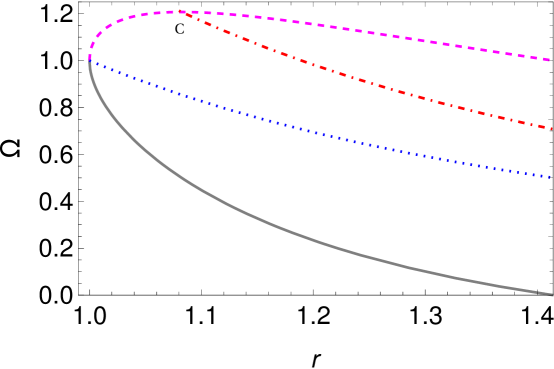
Figure 1: Variation of $\Omega$ (unit of ‘length^-1’) versus $r$ (unit of ‘length’) for $A=B=1$. $\Omega$ can take values only in the range: $(\Omega_{-},\Omega_{+})$. $\Omega_{+}$ and $\Omega_{-}$ (unit of ‘length^-1’) are in dashed magenta and solid gray respectively and are plotted specifically inside the ergoregion, as a function of $r$. It is seen that $\Omega_{\pm}$ meet at the horizon. The dotted blue line stands for the frequency of ZAMO (Zero Angular Momentum Observer), i.e., $q=0.5$. The orbital frequency, i.e., $\Omega_{\phi}=r_{E}/r^{2}$ (see Eq.39) which is indicated by the dot-dashed red curve, crossed over the $\Omega_{+}$ curve at point ‘C’. It signifies that the observer moving with $\Omega_{\phi}$ cannot continue its motion after reaching at the orbit $r=r_{C}$ which corresponds to the particular point ‘C’.

Fig.1 shows that the test spin can take any value of $\Omega$ which is fallen between the dashed magenta and the solid gray curves. One intriguing feature is that the orbital frequency $\Omega_{\phi}$ (see Eq.39 of Appendix A) becomes equal to $\Omega_{+}$ at point ‘C’ cbgm2 . The corresponding radius of the orbit ($r=r_{C}$) is

$$r_{C}=\sqrt{2r_{E}(r_{E}-B)}.$$ (17)

Therefore, a test spin with $\Omega_{\phi}$ is unable to continue its motion at $r\leq r_{C}$ whereas it is possible for $r>r_{C}$. As we have already mentioned, one can note that the test spin can easily continue its motion with any value of $\Omega$ within the range : $\Omega_{-}<\Omega<\Omega_{+}$ in the region $r>r_{H}$. Fig.1 also reveals that the $\Omega_{\pm}$ meet at the horizon with the frequency

$$\Omega_{H}=\frac{B}{r_{H}^{2}}.$$ (18)

Substituting the expression of $\Omega$ (Eq.16) in Eq.(11) we obtain

$$\Omega_{p}=-\frac{2B(1-2q+2q^{2})\sqrt{r^{2}-A^{2}}-(1-2q)(r^{2}-2A^{2})}{4q(1-q)r^{2}\sqrt{r^{2}-A^{2}}}~{},$$ (19)

demonstrating that the spin precession frequency ($\Omega_{p}$) becomes arbitrarily large as it approaches to the horizon ($r\rightarrow A$) for all values of $q$ except $q=0.5$. One should note that Eq.(19) is not valid on the horizon ($r=r_{H}$) as $K$ (Eq.4) must turn null on it.

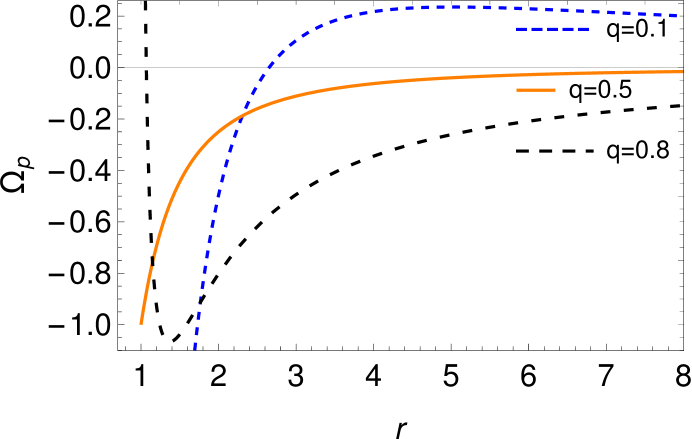
Figure 2: Variation of $\Omega_{p}$ (unit of ‘length^-1’) versus $r$ (unit of ‘length’) for $A=B=1$. It shows that the spin precession frequency $\Omega_{p}$ becomes arbitrarily large as it approaches to the horizon for any value of $q$ whereas $\Omega_{p}$ is finite for $q=0.5$ at $r\rightarrow r_{H}$.

We can see the evolution of the spin precession frequency ($\Omega_{p}$) of a test spin from Fig.2 which is plotted for three consecutive values of $q:0.1,~{}0.5$ and $0.8$. We have taken $A=B=1$ (in the unit of length) which means that the radius of event horizon $r_{H}=A=1$ and radius of the ergoregion $r_{E}=\sqrt{2}$. It can be seen from the figure that $\Omega_{p}$ vanishes for a particular value of $r=r_{0}$ except for $q=0.5$. The value of $r_{0}$ for these cases can be calculated using Eq.(19) and setting $\Omega_{p}|_{r=r_{0}}=0$, which comes out as

$$r_{0}|_{(0<q<0.5)} = \frac{\sqrt{2Y}}{1-2q}~{}\left[Y+B(1-2q+2q^{2})\right]^{\frac{1}{2}}$$ (20)

$${\rm and}$$

$$r_{0}|_{(0.5<q<1)} = \frac{\sqrt{2Y}}{1-2q}~{}\left[Y-B(1-2q+2q^{2})\right]^{\frac{1}{2}}$$ (21)

where, $Y=\left[r_{E}^{2}~{}(1-2q)^{2}+4q^{2}B^{2}~{}(1-q)^{2}\right]^{\frac{1}{2}}$. Eq.(20) is valid for $0<q<0.5$ and Eq.(21) is valid for $0.5<q<1$. This means that even the spacetime possesses a non-zero angular velocity ($\Omega_{a}\neq 0$ or $B\neq 0$), the test spin does not precesses at a particular orbit of radius $r_{0}$. The dashed blue curve of Fig. 2 shows that the spin precession frequency ($\Omega_{p}$) first increases with decreasing of $r$, then it becomes maximum (at $r=r_{p}$) and decreases to zero at $r=r_{0}$ for $q=0.1$. Surprisingly, it becomes ‘negative’ in the region $r_{H}<r<r_{0}$, which means that the spin precesses in the reverse direction after crossing the $r=r_{0}$ orbit. The same feature could be seen for all values of $q$ within the range $0<q<1/2$. Moreover, as $q$ increases, $r_{0}$ shifts in the outward direction and the region ($r_{H}<r<r_{0}$) of the ‘negative precession frequency’ becomes broader and broader. For $q\rightarrow 0^{+}$, $r_{0}\rightarrow\sqrt{2r_{E}~{}(r_{E}+B)}$ which is always greater than $r_{H}=A$ which means that it is always possible to get ‘negative precession frequency’ region for any value of $q~{}:~{}0<q<1/2$.

Now, if we consider the value of $q$ as $0.8$, the precession frequency curve will show a similar feature as occurs for the first case (i.e., $0<q<0.5$). The only difference is that the spin precesses in the opposite direction comparing to the $q<0.5$ cases and it is evident from the dashed black curve of the figure. We point out that the similar trend of the plot could be found for all values of $q:0.5<q<1$, i.e., the precession frequency increases with decreasing of $r$, becomes maximum and then decreases to zero at $r=r_{0}$ (the value of $r_{0}$ can be calculated using Eq.(21) in this case). As $q$ increases, the value of $r_{0}$ shifts in the outward direction but the maximum value of $r_{0}$ will be $r_{0}\rightarrow\sqrt{2r_{E}~{}(r_{E}-B)}$ for $q\rightarrow 1^{-}$. In this case, the value of $r_{0}$ is always greater than $r_{H}$. Therefore, we should get a ‘positive precession frequency’ region ($r_{H}<r<r_{0}$) for any value of $q~{}:~{}0.5<q<1$.

We note that $q=0.5$ (see the dotted blue curve of Fig.1) is a very special case, as $\Omega$ (see Eq.16) reduces to:

$$\Omega|_{q=0.5}=\omega=-\frac{g_{t\phi}}{g_{\phi\phi}}=\frac{B}{r^{2}}=\Omega_{a}.$$ (22)

In this special case, the above expression gives a particular angular frequency $(\omega)$ of the stationary observer computed in the Copernican frame, which is, in fact, the characteristic ZAMO (Zero Angular Momentum Observer) frequency (see the dotted blue line in FIG. 1). In this case, test spins attached to stationary observers regard both $+\phi$ and $-\phi$ directions equivalently, in terms of the local geometry, and see phonons symmetrically mtw . These gyros are non-rotating relative to the local spacetime geometry. The angular momentum of such a ‘locally non-rotating observer’ is zero and is therefore called a zero angular momentum observer (ZAMO), first introduced by Bardeen bd ; mtw . Bardeen et al.bpt showed that the ZAMO frame is a powerful tool in the analysis of physical processes near astrophysical objects. However, Eq.(19) reduces to

$$\Omega_{p}|_{q=0.5}=-\frac{B}{r^{2}}$$ (23)

for $q=0.5$. It is clearly seen that Eq.(23) is independent of $A$, which implies that the spin precession does not diverge at the horizon $r_{H}=A$. It is finite for all values of $r:0<r<\infty$ in principle and the spin precession rate just outside the horizon is a constant which can be expressed as

$$\Omega_{p}|_{(q=0.5,r\rightarrow A)}=-\frac{B}{r_{H}^{2}}=-\Omega_{H}.$$ (24)

Noticeably, it is exactly similar to the expression of $\Omega_{H}$ (see Eq.18) but the direction is opposite. Here, we should note that Eq.(23) diverges only at the ‘singularity’ $r=0$. Therefore, in principle, the following relation holds everywhere of $r:r_{H}<r<\infty$ in the draining bathtub spacetime for $q=0.5$ :

$$\Omega|_{q=0.5}=\Omega_{a}=-\Omega_{p}=\frac{B}{r^{2}}.$$ (25)

One can also conclude that a test spin attached to a ZAMO can easily approach to the event horizon of a ‘Draining Bathtub’ geometry without facing any major difficulty. We also note that the precession frequency ($\Omega_{p}$) of a test spin attached to a ZAMO is same with the angular velocity ($\Omega_{a}$) of the background fluid flow in the draining bathtub geometry but Eq.(25) suggests that their directions are opposite to each other. It is also evident from the solid orange curve of Fig.2 that the spin precession frequency becomes completely ‘negative’ (compared to the first case) for $q=0.5$. Remarkably, $r_{0}$ is absent for $q=0.5$, which means that the spin precession does not vanish except $r\rightarrow\infty$. For $q\neq 1/2$, spin precession frequency shows a divergence feature at $r_{H}=A$, which is similar to the Kerr case ckp .

II.2 At the boundary of ergoregion

Now, it is easily seen from Eq.(19) that the divergence of spin precession can be avoided at the boundary of the ergoregion, contrary to the earlier work reported in Ref.cgm . To cross the boundary of the ergoregion ($r=r_{E}$) the test spin has to acquire the angular velocity as,

$$\Omega|_{r=r_{E}}=\frac{2qB}{r_{E}^{2}}.$$ (26)

Now, substituting the value of $\Omega$ (Eq.(26)) in Eq.(11), we obtain the spin precession rate at the boundary of the ergoregion

$$\Omega_{p}|_{r=r_{E}}=-\frac{4q^{2}B^{2}+r_{E}^{2}(1-2q)}{4q(1-q)Br_{E}^{2}}.$$ (27)

which is finite for the range $0<q<1$ (see also Eq.16), contrary to our previous result (Eq.(9) of cgm ). In a special case, say, for $q=0.5$, the above equation (Eq.(27)) reduces to

$$\Omega_{p}|_{(r=r_{E},q=0.5)}=-\frac{B}{r_{E}^{2}}.$$ (28)

which is same as the angular velocity $(\Omega_{a})$ of the DS flow (Eq.(13) of cgm ) at the boundary of ergoregion.

III Geodetic precession in the ‘non-rotating’ acoustic analogue black hole

It has been shown ckp ; cp that a test spin undergoes precession even in a non-rotating spacetime, if it rotates with a non-zero angular velocity $\Omega$. Therefore, the similar incident can happen in the non-rotating acoustic spacetime also. For $B\rightarrow 0$, the metric (Eq.10) reduces to

$$ds_{\rm DB}^{2}|_{B=0}=-\left(1-\frac{A^{2}}{r^{2}}\right)dt^{2}+\left(1-\frac{A^{2}}{r^{2}}\right)^{-1}dr^{2}+r^{2}~{}d\phi^{2}$$ (29)

and the flow is characterized by the radial component of the fluid velocity potential

$$\vec{v}_{b}|_{B=0}=-\frac{A}{r}~{}\hat{r}~{}.$$ (30)

Though the fluid flow (see Eq.29) does not exactly mimics the Schwarzschild geometry but we are reasonably close to it visser . However, using Eq.(19) for $B\rightarrow 0$, one can easily obtain the spin precession frequency in the non-rotating acoustic analogue spacetime (Eq.29). This turns out as:

$$\Omega_{p}|_{B=0}=-\Omega~{}\frac{r^{2}-2A^{2}}{r^{2}-A^{2}-\Omega^{2}r^{4}}.$$ (31)

where $\Omega$ is not necessarily to be a function of $r$, rather it can take any finite value so that $K$ remains timelike. Now, if the test spin moves along the circular geodesic, $\Omega$ should be the orbital frequency, i.e., $\Omega_{\phi}=A/r^{2}$ (see Eq.(39) of Appendix A for the derivation). For this particular angular velocity, Eq.(31) reduces to

$$\Omega_{p}|_{(B=0,\Omega=A/r^{2})}=-\Omega=-\frac{A}{r^{2}}.$$ (32)

Eq.(32) gives the precession frequency in the Copernican frame, computed with respect to the proper time $\tau$ which is related to the coordinate time $t$ via $d\tau=\sqrt{1-\frac{2A^{2}}{r^{2}}}~{}dt$. Therefore, the precession frequency in the coordinate basis should be written as

$$\Omega^{\prime}=-\frac{A}{r^{2}}\sqrt{1-\frac{2A^{2}}{r^{2}}}.$$ (33)

Now, the difference of $\Omega_{\phi}$ and $\Omega^{\prime}$ could be written as

$$\Omega_{dS}=\Omega_{\phi}-\Omega^{\prime}=\frac{A}{r^{2}}\left(1+\sqrt{1-\frac{2A^{2}}{r^{2}}}\right).$$ (34)

which is identified as the analogous of de-Sitter/geodetic precession chiba ; kro in the non-rotating Schwarzschild black hole, as mentioned in section IV C of Ref. ckp and the Introduction of this paper.

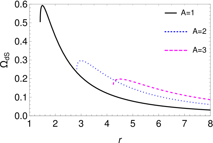
Figure 3: Variation of geodetic precession $\Omega_{dS}$ (unit of ‘length^-1’) versus $r$ (unit of ‘length’) for the non-rotating acoustic blacks hole with different $A$ values. It shows that the precession frequency $\Omega_{\rm dS}$ initially increases, achieves a peak value and then decreases (until it reaches to the orbit of radius $r=\sqrt{2}A$), as the gyro approaches the horizon.

One intriguing behaviour that emerges is, the de-Sitter/geodetic precession frequency ($\Omega_{\rm dS}$) of the test gyro initially increases, achieves a peak value at $r=r_{\rm peak}$, then decreases and discontinues for $r<\sqrt{2}A$, as it approaches to the horizon (see Fig.3). The similar feature cannot occur for Schwarzschild black hole, as the ISCO (innermost stable circular orbit) is located at $r_{\rm ISCO}=6M$ in this case. On the other hand, the stable circular orbits exist everywhere (i.e., $r\geq r_{H}$) in the DS black hole, as is pointed out in Appendix A and therefore gyro can approach the horizon using the stable orbits. However, the gyro does not show geodetic precession for $r<\sqrt{2}A$ as Eq.(34) becomes imaginary for those values of $r$. Eq.(17) also reveals that the orbit of radius $r=\sqrt{2}A$ coincides with $r_{C}$ for $B=0$, which is null. Therefore, the test gyro could not be able to continue its stable ‘geodesic’ motion in those circular orbits which are located at : $A<r\leq\sqrt{2}A$, although those orbits are mathematically stable (see Appendix A). However, as we have mentioned that the geodetic precession frequency becomes maximum at $r=r_{\rm peak}$, one can obtain $r_{\rm peak}=1.5A$ differentiating Eq.(34) with respect to $r$ and setting it to zero for $r=r_{\rm peak}$. Thus, the maximum geodetic precession frequency achieved by a gyro at $r=1.5A$ would be :

$$\Omega^{\rm max}_{\rm dS}|_{r=1.5A}=\frac{16}{27A}\approx 0.593A^{-1}.$$ (35)

IV Observational Prospects

The crucial requirement in the fluid with phonon excitations is the existence of an anisotropy which embodies a precessing gyroscope. In general, this is impossible for a phonon fluid, since phonons do not carry any spin. However, as argued by Garanin and Chudnovsky garanin2015 , circular shear deformations in rotating systems like the DS induces an anisotropy at the classical level in the background fluid. The entire system is of course rotationally invariant, which implies that the shear anisotropy must have a compensation. If the lattice deformation caused by the shear induces a phonon spin through a magnetic Raman spin-phonon interaction, this provides for a mechanism to compensate the shear anisotropy. Recently, Zhang and Niu zhang2014 have argued that this indeed happens in certain paramagnetic materials, providing the possibility of a phonon spin. The question remains as to whether this magnetic effect can be replicated in condensate systems with atoms in the hydrodynamic approximation.

A very different idea is the possibility of an acoustic analogue black hole in an active nematic fluid with bacteria swimming in it. One can associate with these bacteria an orientation (‘polarization’) which introduces an intrinsic degree of anisotropy. Typically, this orientation has a time dependence described by giomi ; bkm

$$[\partial_{t}+{\bf v}\cdot\mathbf{\nabla}]p_{i}+\omega_{ij}p_{j}\\ =\delta_{ij}^{T}\left[\lambda u_{jk}p_{k}+\kappa\nabla^{2}p_{j}\right]~{}$$ (36)

with $\gamma^{\prime},\kappa,\lambda$ being constants, $\delta_{ij}^{T}=\delta_{ij}-p_{i}p_{j}$ being the transverse projection operator$~{},~{}u_{ij}\equiv(\partial_{i}v_{j}+\partial_{j}v_{i})/2~{},{\bf v}=\vec{v_{b}}+\epsilon\vec{v_{1}}$ with $\epsilon<<1$, $\omega_{ij}\equiv(\partial_{i}v_{j}-\partial_{j}v_{i})/2$, and $D_{ij}$ being the effective diffusion tensor governing orientation-dependent diffusion of active nematics and is given by

$$D_{ij}=D(\delta_{ij}-\xi p_{i}p_{j})~{}$$ (37)

where $D$ is the diffusion constant and $\xi$ is another constant related to how much diffusion is influenced by the alignment of active particles. The parameter $|\lambda|$ measures the alignent of the swimming bacteria to a shear flow in the background fluid. The energy lost due to deforming the polarization field of the particles generated by the aligning interactions between individual particles is represented in the last term in right hand side of Eq. (36). In the limit of low background concentration of active particles (bacteria), the active particles may serve as freely-precessing gyroscopes, provided one can ignore their self-interaction. In this case, the dynamic behaviour of the orientation can be graphically represented as in Fig.4 (or, Fig.2(a) of bkm ).

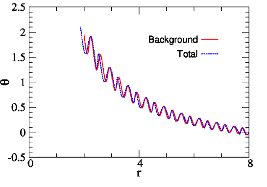
Figure 4: Dynamics of the orientation $\theta$ of active particles with radial coordinate $r$; with $\omega=0.001,A=1,B=10,\epsilon=0.1$. The initial conditions are $x=8,y=0,\theta=0$.

It is obvious that there is marked monotonic functional dependence on the radial distance from the ergosphere. This is precisely what may be quite useful in an accurate measurement of the Lense-Thirring frequency without invoking any weak field approximation. While we no longer claim that the precession frequency diverges on the ergosphere, there is still a substantial enhancement outside the ergoregion. This is where laboratory measurements are the most practicable.

V Conclusions and discussions

We have derived the exact spin precession frequency in the $(2+1)$D stationary and axisymmetric spacetime. From this general formulation, we have shown that the spin precession frequency becomes arbitrarily large as it approaches to the horizon. We have also shown that a test spin attached with the ZAMO can reach close to the horizon of the draining sink geometry without facing any major problem, i.e., its precession frequency remains finite. Contrary to our earlier work cgm , it has been shown here that a test spin can cross the boundary of the ergoregion of an acoustic black hole with a finite precession frequency, if the spin possesses a non-zero finite angular velocity $\Omega$ in a particular range. We note that the results in Ref.cgm was a special case of this general formalism and valid only for the test spin attached to a static observer.

The notion of the test spin in the $(2+1)$D acoustic analogue spacetime has been described in the Introduction but one can question that how the ‘test spin’ acquires the various values of $\Omega$ which has been specified in Eq.(16). Though the phonon-magnon interactions with possible spin-dependent coupling to phonons in spinor condensate are yet to be observed, one can speculate that the coupling should be different for different ionic crystals, discussed in section 5.1 of cgm . This coupling parameter of a particular ionic crystal could be parameterized with the parameter $q$ of this paper. Moreover, in a very recent article bps , an effective magnetic interaction due to the curvature coupling of the quasiparticles has been obtained, which could be think as an equivalent to the ‘spin-gravity coupling’ in the strong gravity regime. One can try to parametrize the notion of curvature coupling using the parameter $q$.

Finally, the very recent assay bkm on discerning an acoustic black hole analogue in an active nematic fluid, raises very interesting prospects of an accurate measurement of the Lense-Thirring precession due to acoustic inertial frame dragging. If issues regarding viscosity in such fluids can be dealt with by lowering the concentration, so that bacteria may indeed propagate with the speed of the fluid, then experimental viability of this very novel, interdisciplinary approach to observation of the full effect of ‘acoustic spin precession’ is perhaps the best of all methods attempted.

Appendix A Derivation of some important observables in DS black hole

In section II, we have derived the general spin precession frequency of a test spin in the $(2+1)$ DS geometry. We already know that a test spin does not move along the geodesic in general hoj ; abk . The spin moves along an arbitrary timelike Killing vector field $K$. In general relativity, the behaviour of a spin is different in the strong gravity regime due to the spin-gravity coupling. This coupling is negligible in the weak gravity regime and that’s why one can assume that the test spin moves along a geodesic jh in the weak gravity regime. This is indeed a fair assumption. Therefore, at a reasonably large distance from the horizon of the draining sink, we can consider that the test spin rotates in a circular ‘geodesic’ and we can derive the orbital frequency ($\Omega_{\phi}$) as well as the radial epicyclic frequency ($\Omega_{r}$) experienced by it. From the general expression of the orbital frequency

$$\Omega_{\phi}=\dot{\phi}/\dot{t}=d\phi/dt=\left[-\partial_{r}g_{t\phi}\pm\sqrt{(\partial_{r}g_{t\phi})^{2}-\partial_{r}g_{tt}~{}\partial_{r}g_{\phi\phi}}\right]/\partial_{r}g_{\phi\phi}$$ (38)

we obtain the orbital frequency in the DS geometry (see Eq.10) as cgm

$$\Omega_{\phi}=\frac{r_{E}}{r^{2}}.$$ (39)

In this spacetime, the proper angular momentum ($l$) is written as :

$$l=\frac{L}{E} = -\frac{g_{t\phi}+\Omega_{\phi}g_{\phi\phi}}{g_{tt}+\Omega_{\phi}g_{t\phi}}$$ (40)

$$= \frac{r^{2}~{}(r_{E}-B)}{(r^{2}-r_{E}^{2}+Br_{E})}.$$ (41)

Now, the general expression for calculating the radial ($\Omega_{r}$) epicyclic frequency is cbgm ; cpjcap

$$\Omega_{r}^{2}=\frac{(g_{tt}+\Omega_{\phi}g_{t\phi})^{2}}{2~{}g_{rr}}\left[\partial_{r}^{2}\left({g_{\phi\phi}}/{Y}\right)+2l~{}\partial_{r}^{2}\left({g_{t\phi}}/{Y}\right)+l^{2}~{}\partial_{r}^{2}\left({g_{tt}}/{Y}\right)\right]$$ (42)

where

$$Y=g_{tt}g_{\phi\phi}-g_{t\phi}^{2}=A^{2}-r^{2}.$$ (43)

Using Eq.(42) square of the radial epicyclic frequency can be obtained as :

$$\Omega_{r}^{2}=\frac{4r_{E}^{2}(r_{E}-B)^{2}}{r^{6}}=\frac{4}{r^{2}}~{}\Omega_{\phi}^{2}~{}(r_{E}-B)^{2}.$$ (44)

It is well-known to us that the square of the radial epicyclic frequency is equal to zero at the innermost stable circular orbit (ISCO) and it is negative for the smaller radius, which shows the radial instabilities for orbits with radius smaller than the ISCO. Interestingly, it can be seen from Eq.(44) that the stable circular orbits exist everywhere in this draining sink spacetime for any value of $r\geq r_{H}$. “Innermost” is not applicable here. $\Omega_{r}^{2}$ could not be negative for any value of $r$ and thus radial instability is completely absent in this spacetime. Now, the periastron precession rate or precession rate of the orbit can be calculated as

$$\Omega_{per}=\Omega_{\phi}-\Omega_{r}=\Omega_{\phi}\left[1-\frac{2}{r}(r_{E}-B)\right].$$ (45)

Therefore, it may also be possible to see the non-zero precession of the phonon orbit in the DS geometry, so long as one restricts observation to the region outside the horizon.

Acknowledgements : One of us (CC) thanks Oindrila Ganguly for useful discussions on this topic. CC also gratefully acknowledges support from the National Key R&D Program of China (Grant No. 2016YFA0400703) and the National Natural Science Foundation of China (Grant No. 11750110410).

References

- (1) K. Sakina, J. Chiba, Phys. Rev. D 19, 2280 (1979)
- (2) K. D. Krori, R. Bhattacharjee, S. Chaudhury, Phys. Rev. D 24, 3044 (1981)
- (3) N. Straumann, General Relativity with applications to Astrophysics, Springer, Berlin (2009)
- (4) C. Chakraborty, P. Pradhan, Eur. Phys. J. C 73, 2536 (2013)
- (5) C. Chakraborty, K. P. Modak, D. Bandyopadhyay, Astrophys. J. 790, 2 (2014)
- (6) C. Chakraborty, Eur. Phys. J. C 75, 572 (2015)
- (7) D. Chatterjee, C. Chakraborty, D. Bandyopadhyay, JCAP 01(2017)062
- (8) S. Mukherjee, S. Chakraborty, Phys. Rev. D 97 (2018) 124007
- (9) C. Chakraborty, P. Kocherlakota, M. Patil, S. Bhattacharyya, P. S. Joshi, A. Królak, Phys. Rev. D 95, 084024 (2017)
- (10) C. Chakraborty, P. Kocherlakota, P. S. Joshi, Phys. Rev. D 95, 044006 (2017)
- (11) P. Kocherlakota, P. S. Joshi, S. Bhattacharyya, C. Chakraborty, A. Ray, S. Biswas, MNRAS 490, 3262 (2019)
- (12) C. Chakraborty, P. Majumdar, Class. Quantum Grav. 31, 075006 (2014)
- (13) W. Unruh, Phys. Rev. Lett. 46, 1351 (1981)
- (14) S. Basak, P. Majumdar, Class. Quantum Grav. 20, 3907 (2003)
- (15) J. Steinhauer, Nature Physics 12, 959 (2016)
- (16) T. Torres et al., Nature Physics 13, 833 (2017)
- (17) L. Liao et al., Phys. Rev. A 99, 023850 (2019)
- (18) C. Chakraborty, O. Ganguly, P. Majumdar, Ann. Phys. (Berlin) 530, 1700231 (2018)
- (19) L. Zhang, Q. Niu, Phys. Rev. Lett. 112, 085503 (2014)
- (20) T. Ray, D. K. Ray, Phys. Rev. 164, 420 (1967).
- (21) D. A. Garanin, E. M. Chudnovsky, Phys. Rev B 92 024421 (2015)
- (22) C. J. Pethick, H. Smith, Bose-Einstein Condensation in Dilute Gases, 2nd ed., Cambridge University Press, (2008)
- (23) A. L. Fetter, Rev. Mod. Phys. 81, 648 (2009)
- (24) A. Banerjee, R. Koley, P. Majumdar, arXiv: 1808.01828 [gr-qc] (2018).
- (25) T. Torres, S. Patrick, M. Richartz, S. Weinfurtner, arXiv:1811.07858 [gr-qc] (2018)
- (26) C. Chakraborty, S. Bhattacharyya, JCAP 05(2019)034
- (27) C. W. Misner, K. S. Thorne, J. A. Wheeler, Gravitation, W. H Freeman Company (1973)
- (28) J. M. Bardeen, Astrophys. J. 162, 71 (1970)
- (29) J. M. Bardeen, W. H. Press, S. A. Teukolsky, Astrophys. J. 178, 347 (1972)
- (30) M. Novello, M. Visser, G. Volovik, Artificial Black Holes, World Scientific, Singapore (2002)
- (31) L. Giomi, T. B. Liverpool, M. C. Marchetti, Phys. Rev. E 81, 051908 (2010)
- (32) P. Banerjee, S. Paul, T. Sarkar, arXiv:1712.05230v2 [gr-qc] (2017)
- (33) S. A. Hojman, F. A. Asenjo, Class. Quantum Grav. 30, 025008 (2013)
- (34) C. Armaza, M. Banados, B. Koch, Class. Quantum Grav. 33, 105014 (2016)
- (35) J. B. Hartle, Gravity:An introduction to Einstein’s General relativity, Pearson (2009)
- (36) C. Chakraborty, P. Pradhan, JCAP 03(2017)035
- (37) C. Chakraborty, S. Bhattacharyya, Phys. Rev. D 98, 043021 (2018)