Conductivity in the square lattice Hubbard model at high temperatures: importance of vertex corrections

Abstract

Recent experiments on cold atoms in optical lattices allow for a quantitative comparison of the measurements to the conductivity calculations in the square lattice Hubbard model. However, the available calculations do not give consistent results and the question of the exact solution for the conductivity in the Hubbard model remained open. In this letter we employ several complementary state-of-the-art numerical methods to disentangle various contributions to conductivity, and identify the best available result to be compared to experiment. We find that at relevant (high) temperatures, the self-energy is practically local, yet the vertex corrections remain rather important, contrary to expectations. The finite-size effects are small even at the lattice size $4\times 4$ and the corresponding Lanczos diagonalization result is therefore close to the exact result in the thermodynamic limit.

Theoretical study of transport in condensed matter systems with strong interactions is very difficult. In many cases there are no long-lived quasi-particles, and the conventional Boltzmann theory of transport provides little insight. Progress can only be made using bona fide many-body approaches to simplified lattice models or effective field theories, where approximations are made in a controlled manner. Terletska et al. (2011); Deng et al. (2013); Xu et al. (2013); Vučičević et al. (2015); Pakhira and McKenzie (2015); Perepelitsky et al. (2016); Kokalj (2017); Huang et al. (2018); Hartnoll et al. (2018) Even then, as only a few specifics of a real system enter the model, the comparison to relevant experiments can only be made at a qualitative level. This changed very recently, when Ref. Brown et al., 2019 reported a measurement of transport in a quantum simulator of the fermionic Hubbard model in two dimensions (2D). The experiment is performed on cold lithium atoms in an optical lattice, a controllable setup free from disorder, phonons and other complications of realistic materials. It is well justified to compare at the quantitative level such experimental result for conductivity with the Hubbard model calculations.

Ref. Brown et al., 2019 found that two state-of-the-art methods namely the finite-temperature Lanczos method (FTLM) and the dynamical mean field theory (DMFT) give conductivities that differ by up to a factor $\frac{3}{2}$, and only FTLM shows a solid agreement with the experiment. At high temperatures $T\gtrsim t$ relevant to these observations (for instance, in cuprates where the hopping parameter $t\approx 0.3$eV the corresponding temperature is well above the melting temperature) one expects the correlation lengths to be short, and the approximations made in the two methods to apply. Our aim is to reveal the physical origin of this discrepancy and to establish a numerically exact solution in the regime $T/t\gtrsim 1$ relevant for optical lattice experiments, as well as other narrow band systems, such as organic superconductors Powell and McKenzie (2011), low temperature phase of TaS₂ Rossnagel and Smith (2006), twisted bilayer graphene Cao et al. (2018), and monolayer transition metal dichalcogenides Coleman et al. (2011), such as 1T-NbSe₂ Nakata et al. (2016).

It is useful to recall that the mentioned numerical methods belong to two distinct general approaches: $A$) one solves an isolated finite cluster of lattice sites, as representative of the thermodynamic limit; Trivedi et al. (1996); Kokalj (2017); Huang et al. (2018) $B$) one solves an effective, self-consistently determined “embedded” cluster, which provides propagators of infinite range, yet limits the range of electronic correlations. Biroli and Kotliar (2002); Maier et al. (2005); Kotliar et al. (2006); Gull et al. (2011); LeBlanc et al. (2015); Ayral and Parcollet (2016); Ayral et al. (2017); Vučičević et al. (2018); Rohringer et al. (2018) The diagrammatic content of the self-energy in the two approaches is sketched in Fig. 1a. Approach $B$ captures longer distance quantum fluctuations, and is therefore assumed to converge more quickly with cluster size at the price of an iterative solution of the (embedded) cluster, as opposed to the “single-shot” calculation in the approach $A$. FTLM solves a $4\times 4$ isolated cyclic cluster and belongs to $A$. DMFT is an embedded cluster calculation ($B$) with the cluster size one, and therefore it approximates the self-energy by a purely local quantity.

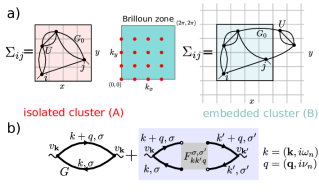
Figure 1: (a) Illustration of the type of self-energy diagrams that are captured by isolated cluster and embedded cluster (in particular cellular DMFT), and the respective difference in the Brillouin zone (discrete vs. continuous). (b) Separation of a susceptibility into the bubble and the vertex corrections part.

Therefore, there are three possible sources of discrepancy between the DMFT and FTLM results for resistivity: (i) non-local correlations which are encoded in the non-local corrections to self-energy, present in FTLM but beyond the DMFT approximation; (ii) quantum fluctuations at distances beyond the linear size of the FTLM cluster; DMFT captures them through an effective fermionic bath; (iii) vertex corrections, included within FTLM, but neglected within DMFT where one calculates only the bubble contribution . We recall that the two-particle correlation functions can be split into the disconnected part (“the bubble”) and the connected part (“vertex corrections”), as shown in Fig. 1b. The bubble captures only the single-particle scattering off the medium, described by the self-energy which enters the full Green’s function. The collective excitations come from the particle-hole scattering, and are present only in the vertex corrections. Whereas the contribution of the connected part is always important for charge susceptibility  Hafermann et al. (2014); Nourafkan et al. (2019); Krien et al. (2018), in the large dimensionality limit the vertex corrections to conductivity cancel  Khurana (1990) (the full vertex $F$ loses $\mathbf{k}\mathbf{k}^{\prime}$-dependence and the current vertex is odd $v_{-\mathbf{k}}=-v_{\mathbf{k}}$, unlike the charge vertex which is even). In finite dimensions, however, the vertex corrections do contribute to conductivity, as discussed previously in several approximative approaches at low temperatures Lin et al. (2009, 2010); Bergeron et al. (2011); Sato et al. (2012); Lin et al. (2012); Sato and Tsunetsugu (2016); Kauch et al. (2019). Based on the Ward identity one could think that when the correlations are approximately local, the vertex corrections become negligible Bergeron et al. (2011); Lin et al. (2009). We show that this expectation is not satisfiedcom (a), and that despite the non-local self-energy being practically negligible at $T\gtrsim 0.3D$, the vertex corrections still amount for a sizable shift in dc-resistivity. Additionally, we show that long-distance quantum fluctuations have little effect on dc conductivity, thus rendering a $4\times 4$ isolated-cluster calculation sufficient to obtain exact results for the bulk model.

Model. We consider the Hubbard model on the square lattice

$$H=-t\sum_{\sigma,\langle i,j\rangle}c^{\dagger}_{\sigma i}c_{\sigma j}+U\sum_{i}n_{\uparrow i}n_{\downarrow i}-\mu\sum_{\sigma,i}n_{\sigma i},$$ (1)

where $c^{\dagger}_{\sigma i}/c_{\sigma i}$ create/annihilate an electron of spin $\sigma$ at the lattice site $i$. The hopping amplitude between the nearest neighbors is denoted $t$, and we set $D=4t$ as the unit of energy. We also take lattice spacing $a=1$, and $\hbar=e=1$. The density operator is $n_{\sigma i}=c^{\dagger}_{\sigma i}c_{\sigma i}$, the chemical potential $\mu$, and the on-site Hubbard interaction $U$. Throughout the paper, we keep $U=2.5D$, which corresponds to the (doped) Mott insulator regime, and assume paramagnetic solutions with full lattice symmetry.

Figure 2: Charge susceptibility (upper) and dc resistivity (lower) as a function of temperature, at different levels of doping. The color between the curves denotes the physical origin of the difference. Dashed curves denote just the bubble contribution, solid lines the full result.

Formalism. The conductivity is defined in terms of the current-current correlation function

$$\Lambda^{xx}_{\mathbf{q}}(i\nu_{n})\equiv\sum_{i}e^{-i\mathbf{q}\cdot\mathbf{r}_{i}}\int d\tau e^{i\nu_{n}\tau}\langle j^{x}_{i}(\tau)j^{x}_{i=0}(0)\rangle,$$ (2)

where $\tau$ is imaginary time, $i\nu_{n}=2in\pi T$ is bosonic Matsubara frequency, $\mathbf{r}_{i}=(x_{i},y_{i})$ denotes the real-space vector of the site $i$. The current operator $j$ is defined as $j^{x}_{i}=-it\sum_{\sigma}c^{\dagger}_{\sigma i}c_{\sigma,\mathrm{n.n.}(i;x)}+\mathrm{h.c.}$ where $\mathrm{n.n.}(i;x)$ denotes the nearest neighbor in the $x$ direction. We are interested in longitudinal, uniform conductivity $\sigma^{xx}_{\mathbf{q}=0}(\omega)$, so we adopt a shorthand notation $\Lambda(i\nu_{n})\equiv\Lambda^{xx}_{\mathbf{q}=0}(i\nu_{n})$ and $\sigma(\omega)\equiv\sigma^{xx}_{\mathbf{q}=0}(\omega)$. The optical conductivity is given byColeman (2015) $\sigma(\omega)=-(i/\omega)\left[\Lambda(\omega)-\Lambda(\omega=0)\right]$, where $\Lambda(\omega)$ is the analytical continuation of $\Lambda(i\nu_{n})$ to the real axis, i.e. the inverse of the Hilbert transform

$$\Lambda(i\nu)=\frac{1}{\pi}\int d\omega\frac{\mathrm{Im}\Lambda(\omega)}{\omega-i\nu}=\frac{1}{\pi}\int d\omega\frac{\omega\mathrm{Re}\sigma(\omega)}{\omega-i\nu}.$$ (3)

The second equality in Eq. (3) is due to $\mathrm{Im}\Lambda(\omega=0)=0$. The direct-current (dc) conductivity is defined as $\sigma_{\mathrm{dc}}=\mathrm{Re}\sigma(\omega=0)=\mathrm{Im}\Lambda^{\prime}(\omega=0)$, and the dc resistivity is then $\rho_{\mathrm{dc}}=1/\sigma_{\mathrm{dc}}$.

In order to better identify and understand the importance of various processes for the transport, we also calculate the charge susceptibility $\chi_{\mathrm{c}}=d\langle n\rangle/d\mu$, which corresponds to the charge-charge correlation functioncom (b). Both $\chi_{\mathrm{c}}$ and $\Lambda$ and can be separated into the bubble and the vertex corrections partcom (c), Fig. 1. In all quantities, the superscript “disc” denotes the bubble contribution, and the superscript “conn” the vertex corrections part.

Methods $A$. We solve an isolated cyclic $4\times 4$ cluster using the FTLM Jaklič and Prelovšek (2000, 1995) method and both $4\times 4$ and $8\times 8$ using quantum Monte Carlo (the continuous-time interaction-expansion algorithm, CTINTRubtsov and Lichtenstein (2004); Gull et al. (2011)) Both methods yield numerically exact solutions of the representative finite-size model. In FTLM we calculate $\sigma(\omega)$, while CTINT yields $\Lambda(i\nu_{n})$, as well as the self-energy $\Sigma_{ij}(i\omega_{n})$ and the Green’s function $G_{ij}(i\omega_{n})$com (d). Note that both CTINT and FTLM allow for a direct calculation of the full current-current correlation function, and that we need not evaluate the full vertex function $F$ at any stage of the calculation.

In the isolated cluster calculations one faces several finite-size effects stemming from the finite range of the bare electronic propagatorJaklič and Prelovšek (1995, 2000). Most importantly, this not only limits the range of electronic correlations, but also affects the diagrammatic content of short range correlations: diagrams with distant interaction vertices are not captured (Fig. 1). One may see this equivalently in the $\mathbf{k}$-space as a discretization of the Brillouin zone, which affects the internal momentum summations in all self-energy and full vertex diagrams.

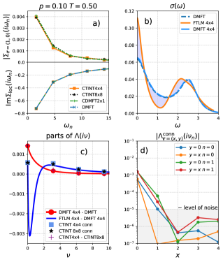
Figure 3: All panels: $p=0.1$, $T=0.5D$. a) Benchmark of self-energy and inspection of its leading non-local component. b) Comparison of the optical conductivity between various methods. c) See text. d) Real-space resolution of the vertex corrections along two spatial directions (CTINT $8\times 8$ result).

Methods $B$. We solve the embedded clusters of size $2\times 1$ and $2\times 2$ within the cellular DMFT scheme (CDMFT)Kotliar et al. (2001) and the $4\times 4$ cluster within the dynamical cluster approximation (DCA) schemeHettler et al. (1998), both using CTINT. (Unlike the isolated cluster case, the bare propagator entering CTINT here takes into account the effective medium.) The single-site DMFT calculations (cluster size $N_{\mathrm{c}}=1$) are done using both the CTINT and the approximative real-frequency numerical renormalization group method (NRG) as impurity solvers.

In CDMFT, an electron can travel infinitely far between two scatterings, but a self-energy insertion in the corresponding diagrammatic expansion can only be of limited range (see Fig. 1). In DCA, the approximation is made in reciprocal space and amounts to allowing the electron to visit $\mathbf{k}$-states otherwise not present in the finite cluster.Vučičević et al. (2018)

Results. Top panels of Fig. 2 show the temperature dependence of $\chi_{\mathrm{c}}$ for several values of doping $p=1-\langle n\rangle$. One sees that in the high-temperature regime $T\gtrsim 0.3D$, the results of different methods (solid curves) all agree and tend toward the atomic limit, as expected for a thermodynamic quantity.

At lower temperatures, the non-local correlations show up. Away from half-filling, FTLM and DCA yield a charge susceptibility that increases with lowering temperature, yet in DMFT, it saturates instead. The enhancement of charge susceptibility at low $T$ comes from the antiferromagnetic fluctuations Kokalj (2017). The difference between the DCA and the DMFT is used to characterize the importance of non-local correlations (green shading). They manifest themselves also in the growth of non-local self-energy at low $T$ (thin dashed-dotted lines). The DCA and the FTLM result do not completely coincide; the difference (pink shading) comes from the longer-distance quantum fluctuations. The discretization of the Brillouin zone in FTLM can be somewhat ameliorated by the twisted-boundary conditions scheme (TBC) Poilblanc (1991). As expected, TBC is closer to DCA (black line), but one needs a better method to capture the full effect of longer-range processes.

We have also evaluated separately the bubble contribution $\chi^{\mathrm{disc}}$ to $\chi_{c}$ (dashed lines) and observe it is substantially larger than the full result $\chi_{c}$.

Bottom panels of Fig. 2 show the temperature dependence of resistivity $\rho_{\mathrm{dc}}$ as calculated from the bubble term in the DMFT (dashed line) and the full result from FTLM (solid line). Strikingly, even in the temperature range $T\gtrsim 0.3D$ where the behavior of $\chi_{c}$ collapsed to that of the atomic limit, the DMFT and FTLM are shown to yield significantly different results with a lower value of resistivity found in the FTLM.

To understand the origin of this difference we take a closer look of the data at $T=0.5$, $p=0.1$ that we show in Fig. 3. In panel a) we compare the self-energies found in the DMFT, CDMFT 2x1 and the CTINT calculation for the isolated $4\times 4$ and $8\times 8$ clusters. Not only is the nearest neighbor self-energy (top) found to be two orders of magnitude smaller than the local one (bottom), but also the local parts of the self-energies show excellent agreement. Thus, neither non-local correlations (neglected in DMFT) nor long-range processes (neglected in $4\times 4$) play an important role for the self-energy at this temperature.

Might long-range processes play a more important role for the conductivity? One can readily investigate the role of long-range processes for the bubble part of the conductivity. This is done by calculating the conductivity in the DMFT formulated for the $4\times 4$ lattice, which amounts to discretizing the Brillouin zone (in both the self-consistency condition, and internal bubble summation (Fig. 1b). Fig. 3b compares the optical conductivity obtained in this way (denoted by DMFT $4\times 4$) to the infinite lattice DMFT result and to the FTLM one. The DMFT and the DMFT $4\times 4$ are close: the long-range processes clearly do not account for the discrepancy between the DMFT and the FTLM either. The most of the difference between the DMFT and the FTLM conductivity thus comes from the vertex corrections.

To further verify this result we have evaluated the current-current correlation function $\Lambda(i\nu_{n})$ also in CTINT $4\times 4$, and deduced the connected part by $\Lambda^{\mathrm{conn}}(i\nu_{n})=\Lambda(i\nu_{n})-\Lambda^{\mathrm{disc}}(i\nu_{n})$, which is shown by the blue squares in Fig. 3c. These points fall on the blue line which is obtained by the Hilbert transform to the imaginary axis (Eq. 3) of the difference in $\sigma(\omega)$ between the FTLM and the DMFT $4\times 4$ (see Supplemental Material (SM) for details and other $p,T$). Note that the magnitude of $\Lambda^{\mathrm{conn}}$ at the Matsubara frequencies is rather small, consistent with the Ward identity $\Lambda^{\mathrm{conn}}(i\nu=0)\sim\sum_{\mathbf{k}}v_{\mathbf{k}}\sum_{i\omega_{n}}G^{2}_{\mathbf{k}}(i\omega_{n})\partial_{k_{x}}\Sigma_{\mathbf{k}}(i\omega_{n})$, that associates $\Lambda^{\mathrm{conn}}(i\nu_{0})$ with $\partial_{k_{x}}\Sigma_{\mathbf{k}}$ (see SM for further discussion). The conductivity is, however, determined by the slope, $-\partial_{\nu}\mathrm{Re}\Lambda(i\nu)|_{\nu=0^{+}}=\sigma(\omega=0)=\sigma_{\mathrm{d}c}$, and the contribution from $\Lambda^{\mathrm{conn}}$ is not small, but comparable to the bubble term. The slope of the red line which corresponds to the DMFT $4\times 4$ - DMFT difference is small, reflecting the practically negligible finite-size effects in the bubble.

The shape of $\Lambda^{\mathrm{conn}}$ is difficult to reconstruct with analytical continuation from noisy data at the Matsubara frequencies (see SM), which we circumvented by using FTML.

Might the impact of vertex corrections change if larger systems are considered? The added longer distance components of $\Lambda^{\mathrm{conn}}_{\mathbf{r}}$ could be sizeable, and even the short distance components might change due to improved diagrammatic content captured by the bigger cluster. We have performed the CTINT $8\times 8$ computation to address this question. In Fig. 3c we compare $\Lambda^{\mathrm{conn}}(i\nu_{n})$ between $4\times 4$ and $8\times 8$ clusters (blue squares and black stars) and observe they are equal within the statistical error bars (about the size of the square symbol). As for the longer distance components, we analyze the vertex corrections term as a function of real-space vector $\Lambda^{\mathrm{conn}}_{\mathbf{r}}(i\nu_{n})$ and present the results in Fig. 3d. Indeed, the values drop rapidly with distance and the range of $\Lambda^{\mathrm{conn}}$ is clearly captured by the $4\times 4$ cluster. Furthermore, the difference in the full $\Lambda$ between $4\times 4$ and $8\times 8$ clusters (purple crosses) appears to coincide with the finite size effects in the bubble (red line/dots) obtained entirely independently with DMFT.

Small finite-size effects are also indicated from a comparison of the frequency moments of FTLM $\sigma(\omega)$ in the high-$T$ limit with the exact values from Ref. Huang et al., 2018, where we find an excellent agreement within $\lesssim 0.2$% (see SM).

It is important to note that apart from reducing the dc resistivity, the vertex corrections have a characteristic effect on the frequency dependence of optical conductivity (see Fig. 3b and SM). The high-frequency peak in $\sigma(\omega)$ obtained from DMFT is centered at precisely $\omega=U=2.5D$. This peak describes single-particle transitions between the Hubbard bands. The inclusion of vertex corrections brings about multi-particle excitations which move this peak towards lower frequencies, as noted previously in a slightly different context (see Refs. Cunningham et al., 2018; Gatti et al., 2007; Vidal et al., 2010).

Conclusions. In the high-temperature $T\gtrsim t$, (doped) Mott insulator regime of the Hubbard model, the single-particle self-energy is almost local, yet the vertex corrections to dc resistivity persist. This finding applies to the optical lattice investigation in Ref. Brown et al., 2019, and explains why the DMFT results disagree with the experiment. On the other hand, we demonstrate that the long-distance quantum fluctuations play a negligible role, and thus the $4\times 4$ isolated cluster becomes representative of the thermodynamic limit. The corresponding FTLM result is therefore close to exact, and is an important benchmark for the experiment in Ref. Brown et al., 2019 and future cold atoms experiments.

We cannot access with the same confidence the regime below $T\sim t$. Determinantal Quantum Monte Carlo algorithms in principle allow access to larger lattices and thus lower temperatures (see Ref. Huang et al., 2018), but the analytical continuation presents a possible source of systematic error which is difficult to detect and estimate (see SM for a detailed analysis using the implementation of Maximum Entropy method taken from Ref. Levy_mem17). Our results highlight the need for developing real-frequency diagrammatic methods, like the one proposed recently in Ref. Taheridehkordi et al., 2019.

Finally, our results suggest that proper account of the vertex corrections is needed at all temperatures. The discrepancies between the experimental observations and the DMFT, such as those observed in the case of hcp-Fe Pourovskii et al. (2014) or in Sr₂RuO₄ Deng et al. (2016) should not be interpreted only in terms of non-local correlations. Very recentlyKauch et al. (2019), this conclusion has been shown to be valid even at much weaker coupling and in various other models.

See pages 1 of supp_mat.pdf See pages 2 of supp_mat.pdf See pages 3 of supp_mat.pdf See pages 4 of supp_mat.pdf See pages 5 of supp_mat.pdf See pages 6 of supp_mat.pdf See pages 7 of supp_mat.pdf