Updated Core Libraries of the ALPS Project

Abstract

The open source ALPS (Algorithms and Libraries for Physics Simulations) project provides a collection of physics libraries and applications, with a focus on simulations of lattice models and strongly correlated electron systems. The libraries provide a convenient set of well-documented and reusable components for developing condensed matter physics simulation codes, and the applications strive to make commonly used and proven computational algorithms available to a non-expert community. In this paper we present an update of the core ALPS libraries. We present in particular new Monte Carlo libraries and new Green’s function libraries.

PROGRAM SUMMARY

Program Title: ALPS Core libraries 2.3
Project homepage: http://alpscore.org
Catalogue identifier: –
Journal Reference: –
Operating system: Unix, Linux, macOS
Programming language: C++11 or later
Computers: any architecture with suitable compilers including PCs, clusters and supercomputers
Licensing provisions: GNU General Public License (GPLv2+)
Classification: 6.5, 7.3, 20
Dependencies: CMake ($\geq 3.1$), Boost ($\geq 1.56$), HDF5 ($\geq 1.8$), Eigen ($\geq 3.3.4$)
Optional dependencies: MPI ($\geq 2.1$), Doxygen
Nature of problem: Modern, lightweight, tested and documented libraries covering the basic requirements of rapid development of efficient physics simulation codes, especially for modeling strongly correlated electron systems.
Solution method: We present C++ open source computational libraries that provide a convenient set of components for developing parallelized physics simulation codes. The library features a short development cycle and up-to-date user documentation.

1 Introduction

The open source ALPS (Algorithms and Libraries for Physics Simulations) project [1, 2, 3, 4] provides a collection of computational physics libraries and applications, especially suited for the simulation of lattice models and strongly correlated systems. The libraries are lightweight, thoroughly tested and documented. The libraries are targeted at code developers who implement generic algorithms and utilities for rapid development of efficient computational physics applications.

Computer codes based on the ALPS (core) libraries have provided physical insights into many subfields of condensed matter. Highlights include nonequilibrium dynamics [5, 6], continuous-time quantum Monte Carlo [7, 8, 9, 10], LDA+DMFT materials simulations [11], simulations of quantum [12] and classical [13] spin systems, correlated boson [14] and fermion [15] models, as well as cuprate superconductivity [16].

In this paper we present an updated and refactored version of the ALPS core libraries. This version introduces a new module to the library: ALPS ALEA, which is designed as a replacement of the previous accumulator framework. It provides significant runtime speed-ups for all of its accumulator types, improved compile times, as well as support for complex random variables, non-linear propogation of uncertainty and statistical hypothesis testing as a way to compare stochastic results (Section 2).

Improvements and bug fixes were made to the existing modules. The Green’s function library was rewritten to be faster and more versatile (Section 3). Section 4 briefly discusses the other components of the library with the corresponding improvements.

An effort was made to make the installation procedure more robust and straight-forward. In Section 5, we list the software packages prerequisite for compiling and installing the library, as well as outline the installation procedure. In Section 6 we specify the ALPS citation policy and license, and in Sections 7 and 8 we summarize the paper and acknowledge our contributors. Additionally, A provides installation examples.

2 ALEA library

The ALEA library (namespace alps::alea) is the next-generation statistics library for Markov chain Monte Carlo calculations in the ALPS core libraries. It is intended to supersede the old accumulators library (namespace alps::accumulators), which is still supported for backwards compatibility. Compared to the old library, ALEA features:

• improved runtime scaling for full binning and logarithmic binning accumulators, which were both reduced from ${\mathcal{O}}(N\log N)$ to ${\mathcal{O}}(N)$ in terms of the number of samples $N$.[17]

• improved runtime performance for vector-valued accumulators due to the use of the Eigen library and the avoidance of the creation of temporary objects.

• improved memory footprint: (a) the use of finalize() semantics avoids duplicating the accumulator’s data when evaluating the mean and variance; (b) computed objects allow creating and adding a new measurement in one step without the need to create a temporary.

• improved full binning procedure allows the retention of more fine-grained data while keeping linear runtime scaling.[17]

• improved compilation times and error messages: (a) the interface was greatly simplified, the metaprogramming logic was removed, and the numerics are now in the compiled library instead of the headers; (b) the compile-time dependence on MPI and HDF5 was removed and superseded by clearly specified interfaces.

• native support for complex random variables, with user choice of computing either circular error bars or an error ellipse.

• support for computing the full covariance matrix.

• support for statistical hypothesis testing [18] as a robust way to compare Monte Carlo results.

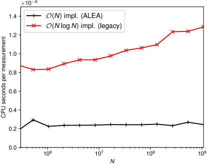
Figure 1: CPU time spent per data point when accumulating $N$ data points of a random vector with $k=100$ components for the legacy accumulators framework (red crosses) and the ALEA library (black plusses).

To illustrate the improvements, we compare the CPU time needed per data point for accumulating the autocorrelation time for a random vector with $k=100$ components between the old accumulators framework and ALEA (Figure 1). One can see that there is both an offset to the scaling, which comes from avoiding temporaries, as well as a better overall ${\mathcal{O}}(N)$ vs. ${\mathcal{O}}(N\log N)$ scaling.

Accumulators

In Monte Carlo simulations, we are interested in obtaining statistical properties of some random vector $X$ with $k$ components by estimating it from a sequence of $N$ samples or “measurements” $x=(x_{1},x_{2}\ldots,x_{N})$. Typically, $N$ is so large that retaining the individual sample points is impossible or at least impractical. ALEA accumulators provide a workaround by retaining only certain aggregates of the measurements by performing reductions over the measurements on the fly, one measurement at a time.

ALEA defines five accumulators, which differ in the stored statistical estimates and associated runtime and memory cost (cf. Table 1). They represent commonly used cases ranging from fast and memory efficient to slow but precise. In all accumulators, size() returns $k$, while count() returns $N$.

ALEA name	old name	time	memory	mean	var	cov	tau	batch
				$\langle x\rangle$	$\sigma_{x}^{2}$	$\Sigma_{x}$	$\tau_{\mathrm{int},x}$	$\bar{x}_{i}$
mean_acc	MeanAccumulator	$Nk$	$k$	✓
var_acc	NoBinningAccumulator	$Nk$	$k$	✓	✓
cov_acc	—	$Nk^{2}$	$k^{2}$	✓	✓	✓
autocorr_acc	LogBinningAccumulator	$Nk$	$k\log N$	✓	✓		✓
batch_acc	FullBinningAccumulator	$Nk$	$Bk$	✓	✓	✓		✓

Table 1: Accumulators in ALEA. Asymptotic complexity ${\mathcal{O}}(\cdots)$ for memory and runtime in terms of sample size $N$, number of components of random vector $k$, and number of bins $B$. Available statistical estimates are marked with “✓”, where $\langle x\rangle$ is the sample mean, $\sigma_{x}^{2}$ is the sample variance, $\Sigma_{x}$ is the sample covariance matrix, $\tau_{\mathrm{int},x}$ is the logarithmic binning estimate for the integrated autocorrelation time, and $\bar{x}_{i}$ are bin means.

Complex variances

In the case of complex random variables, the concept of error bars becomes somewhat ambiguous. ALEA supports two common strategies by admitting an additional Str template argument to var_acc and cov_acc:

• Error with circularity constraint (circular_var): error based on the distance from the mean (circle) in the complex plane. Provides an upper bound to the total error and ignores any error structure in the real and imaginary part of the variable.

• Error ellipse (elliptic_var): Treats the real and imaginary part of a complex variable as two separate random variables, thus creating an error ellipse around the mean in the complex plane. Retains the full error structure in the complex plane and allows one to plot separate error bars for real and imaginary part.

Accumulators and results

Figure 2: Accumulator and result types: finite state machine for accumulator lifecycle. The boxes “empty”, “accumulating” and “finalized” represent the possible states of the accumulator. Calling the method indicated on the edges takes the accumulator from one state to another.

Each accumulator type has a matching result type (e.g., mean_acc has a matching mean_result). Accumulators and results are facade types over a common base type (e.g., mean_data), but differ conceptually and thus have complementary functionality: accumulators support adding data to them, while results allow one to perform transformations, reductions, as well as extracting statistical estimates such as the sample mean.

To obtain a result from an accumulator, the accumulators provide both a result() and a finalize() method. The result() method creates an intermediate result, which leaves the accumulator untouched and thus must involve a copy of the data, while the finalize() method invalidates the accumulator and repurposes its internal data as simulation result (it replaces the sum with the mean and the sum of squares with the variance). A finite state machine for these semantics is shown in Figure 2.

One can not only add a vector of data points to an accumulator, but also a computed object, which creates and adds the data to the accumulator. The result and computed semantics taken together allow one to use ALEA with very large random vectors which may fit in memory only once.

Reductions and serializations

For parallel codes, all results support reduction (averaging over elements) through the reduce() method, which takes an instance of the abstract reducer interface. Depending on the implementation of the reducer, the reduction is performed over different instances (threads, processes, etc.) using MPI, OpenMP, ssh etc. without introducing a hard dependency on any of these libraries.

Similarly, all results support serialization (converting to permanent format) though the serialize() method and deserialization through the deserialize() method, which take an instance of the abstract serializer and deserializer interface, respectively. Depending on the implementation, serialization to HDF5 as well as support for the HPX parallelization framework [19] is provided.

Nonlinear propagation of uncertainty

Transformations of results can be performed using the transform method. The definition of transform, somewhat simplified, is:

⬇

Result transform(Strategy strategy, Function f, const Result &x);

where strategy is a tag denoting the strategy for error propagation, f is the function $f$, and x is the stochastic result.

Care has to be taken to correctly propagate the uncertainties if these functions are non-linear, since neglecting the proper error propagation leads to biasing both the mean and the variance of the transformed result. Several strategies exist for performing these transforms, and we summarize the ones supported by ALEA in Table 2. Similar to the case of the accumulators, there is a tradeoff between computer time required (in particular where $f$ has to be evaluated repeatedly) and requirements on the Result type, such as the presence of binned data.[17]

If $f$ is a linear function, propagation through linear_prop is exact. For non-linear functions on moderate number of components $k$, we suggest the use of Jackknife (jackknife_prop), which strikes a good tradeoff between bias correction and cost. The strategies sampling_prop and bootstrap_prop will be implemented in a later version.

propagation strategy	preimage distribution	mean bias	variance bias	$N_{f}$	requires
					$\langle x\rangle$	$\Sigma_{x}$	$\tau_{x}$	$\bar{x}_{i}$
no_prop	any	$N^{-1}$	—	$1$	✓
linear_prop	Gauss	$N^{-1}$	$1$	$k$	✓	✓	✓
sampling_prop	known	$S^{-\frac{1}{2}}$	$S^{-\frac{1}{2}}$	$S$	✓	✓	✓
jackknife_prop	any	$B^{-2}$	$B^{-2}$	$B$				✓
bootstrap_prop	any	$S^{-\frac{1}{2}}$	$S^{-\frac{1}{2}}$	$S$				✓

Table 2: Common strategies for uncertainty propagation through a function $Y=f(X)$. The preimage distribution is the distribution of $X$. Bias describes the asymptotic $O(\cdots)$ worst-case behavior of the bias on the mean in terms of the bin size $B$, the number of measurements $N$ taken, or the number of samples $S$ used for resampling. $N_{f}$ summarizes the number of function invocations required. The statistical estimates required by each strategy are marked with “✓”. $\langle x\rangle$ is the sample mean, $\Sigma_{x}$ is the sample covariance matrix, $\tau_{x}^{\mathrm{int}}$ is the integrated autocorrelation time, and $\bar{x}_{i}$ are the bin means.

Hypothesis testing

A common task arising in statistical post-processing is to compare a stochastic result with a deterministic one, e.g., when testing the algorithm against known benchmark results, as well as comparing two stochastic results with each other, e.g., when trying to determine whether an iterative procedure has converged. This is usually done by visual inspection or some ad hoc criterion.

Statistical hypothesis testing[18] provides a controlled alternative to these methods. ALEA provides the method test_mean(x, y), which allows for hypothesis testing. If x is a statistical result with proper (co-)variances and y is a benchmark (or vice-versa), test_mean performs Hotelling’s $T^{2}$ test for the following null hypothesis $H_{0}$:[20]

$$H_{0}:\langle x\rangle=y,$$ (1)

whereas if both are statistical results, the null hypothesis

$$H_{0}:\langle x\rangle=\langle y\rangle$$ (2)

is checked. In both cases, an object providing the test score and the corresponding $p$-value is returned, which, roughly speaking, indicates the probability of the two results being in agreement. The $p$-value can then be compared with a suitable threshold $\alpha\in[0,1)$, and one considers the results equal (accepts the null hypothesis) if $p>\alpha$.

3 Green’s function library

The Green’s functions component provides a type-safe interface to manipulate objects representing bosonic or fermionic many-body Green’s functions, self-energies, susceptibilities, polarization functions, and similar objects. From a programmer’s perspective, these objects are multidimensional arrays of floating-point or complex numbers, defined over a set of meshes and addressable by a tuple of indices, each belonging to a grid. Currently, real frequency, Matsubara (imaginary frequency), imaginary time (uniform, power, [21] Legendre [22] and Chebyshev [23]), momentum space, real space, and arbitrary index meshes are supported.

These many-body objects often need to be supplemented with analytic tail information encapsulating the high frequency / short time moments of the Green’s functions, so that high precision Fourier transforms, density evaluations, or energy evaluations can be performed. In addition to this functionality, the Green’s function component supports saving data to and loading it from binary HDF5 files. The UML diagram illustrating the Green’s function classes and their interdependencies is given in Fig. 3.

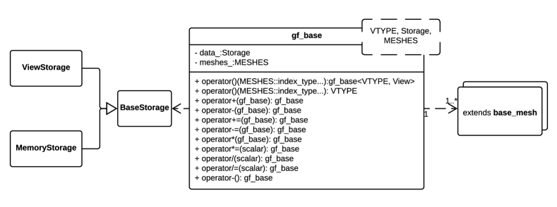
Figure 3: UML class diagram of Green’s function library, indicating the main classes in the Green’s function library. Each box corresponds to a class, and arrows correspond to relationships between classes.

The central class of the Green’s function library is gf_base. This class should be parametrized by the scalar type, the type of storage and the list of meshes (grids). It provides the following basic arithmetic operations:

• Addition/subtraction;

• In-place addition/subtraction;

• Multiplication by a constant.

The addition/subtraction operations can be performed on the Green’s function objects that are defined on the same grid and have the same shape of the data array. There are two possible storage types for this class. The memory storage version of the class is called greenf, whereas the view-based class is called greenf_view. Instead of having only pre-defined Green’s function classes of fixed dimension, we provide a flexible interface that makes it possible to declare Green’s function types of any dimension. The following example defines 4-dimensional Green’s function on Matsubara, arbitrary index, imaginary time and Legendre meshes:

⬇

alps::gf::matsubara_positive_mesh x(100, 10);

alps::gf::index_mesh y(10);

alps::gf::itime_mesh z(100, 10);

alps::gf::legendre_mesh w(100, 10);

greenf<double, alps::gf::matsubara_positive_mesh, alps::gf::index_mesh, alps::gf::itime_mesh, alps::gf::legendre_mesh> g(x, y, z, w);

Using view-storage Green’s function one can easily get access to a part of another Green’s function object using index slicing. This idea is illustrated by the following code,

⬇

alps::gf::matsubara_positive_mesh x(100, 10);

alps::gf::index_mesh y(20);

greenf<double, alps::gf::matsubara_positive_mesh, alps::gf::index_mesh> g(x,y);

// loop over leading index

for(alps::gf::matsubara_positive_mesh::index_type w(0); w<x.extent(); ++w) {

greenf_view<double, alps::gf::index_mesh> g2 = g(w);

// do some operation on the Green’s function view object

// defined on the ’y’ mesh alone

}

In the current implementation we support only a slicing over a set of the leading indices. More details on the Green’s function library can be found in the respective tutorial.

4 Some of the other key library components

In this section, we provide a brief overview of the purpose and functionality of some of the key components comprising the ALPS core libraries. For a more detailed exposition with a working example, see the previous publication[1]. Additional information is available online and as part of the Doxygen code documentation. It should be noted that the components maintain minimal interdependence, and using a component in a program does not bring in other components, unless they are required dependencies, in which case they will be used automatically.

Building a parallel Monte Carlo simulation

A generic Monte Carlo simulation can be easily assembled from the classes provided by the Monte Carlo Scheduler component. The programmer needs to define only the problem-specific methods that are called at each Monte Carlo step, such as methods to update the configuration of the Markov chain and to collect the measured data. The simulation is parallelized implicitly, using one MPI process per chain.

Storing, restoring, and checkpointing simulation results

To store the results of a simulation in a cross-platform format for subsequent analysis, one can use the Archive component. The component provides convenient interface to saving and loading of common C++ data structures (primitive types, complex numbers, STL vectors and maps), as well as of objects of user-defined classes to/from HDF5 [24], which is a universally supported and machine independent data format.

Reading command-line arguments and parameter files

Input parameters to a simulation can be passed via a combination of a parameter file and command line arguments. The Parameters library component is responsible for parsing the files and the command line, and providing access to the data in the form of an associative array (akin to C++ map or Python dictionary). The parameter files use the standard “*.ini” format, a plain text format with a line-based syntax containing key = value pairs, optionally divided into sections.

5 Prerequisites and Installation

To build the ALPS core libraries, any recent C++ compiler can be used; the libraries are tested with GCC [25] 4.8.1 and above, Intel [26] C++ 15.0 and above, and Clang [27] 3.2 and above. The library follows the C++11 standard [28] to facilitate the portability to a wide range of programming environments, including HPC clusters with older compilers. The library depends on the following external packages:

• The CMake build system [29] of version 3.1 and above.

• The Boost C++ libraries [30] of version 1.56.0 and above. Only the headers of the Boost library are required.

• The HDF5 library [24] version 1.8 and above.

• The Eigen library [31] version 3.3.4 and above (can be requested to be downloaded automatically).

To make use of (optional) parallel capabilities, an MPI implementation supporting standard 2.1 [32] and above is required. Generating the developer’s documentation requires Doxygen [33] along with its dependencies.

The installation of the ALPS core libraries follows the standard procedure for any CMake-based package. The first step is to download the ALPS core libraries source code; the recommended way is to download the latest ALPS core libraries release from https://github.com/ALPSCore/ALPSCore/releases. Assuming that all above-mentioned prerequisite software is installed, the installation consists of unpacking the release archive and running CMake from a temporary build directory, as outlined in the shell session example below (the $ sign designates a shell prompt):

⬇

$ tar -xzf ALPSCore-2.3.0.ta#()r.gz

$ mkdir build

$ cd build

$ export ALPSCore_DIR=$HOME/software/ALPSCore

$ cmake -DCMAKE_INSTALL_PREFIX=$ALPSCore_DIR \

-DALPS_INSTALL_EIGEN=yes \

../ALPSCore-2.3.0

$ make

$ make t#()est

$ make install

The command at line 1 unpacks the release archive (version 2.3.0 in this example); at line 4 the destination install directory of the ALPS core libraries is set ($HOME/software/ALPSCore in this example). At line 6 the downloading and co-installation of Eigen library is requested (see  A for more details).

The ALPS core libraries come with an extensive set of tests; it is strongly recommended to run the tests (via make test) to verify the correctness of the build, as it is done at line 9 in the example above.

The installation procedure is outlined in more details in A; Also, the file common/build/build.jenkins.sh in the library release source tree contains a build and installation script that can be further consulted for various build options.

Binary packages are available for some operating systems. On macOS operating system, the ALPS core libraries package can be downloaded and installed from the MacPorts [34] repository, using a command port install alpscore. On GNU/Debian Linux operating system, the ALPS core Debian package is provided by the MateriApps LIVE! project [35] (see [36] for more details).

6 License and citation policy

The GitHub version of ALPS core libraries is licensed under the GNU General Public License version 2 (GPL v. 2) [37] or later. The older ALPS license under which previous versions of the code were licensed [4] has been retired. We kindly request that the present paper be cited, along with any relevant original physics or algorithmic paper, in any published work utilizing an application code that uses this library.

7 Summary

We have presented an updated and repackaged version of the core ALPS libraries, a lightweight C++ library, designed to facilitate rapid development of computational physics applications, and have described its main features.

The new version contains the next-generation statistics library ALEA, a major overhaul of the Green’s function library as well as updates to other components.

8 Acknowledgments

Work on the ALPS library project is supported by the Simons collaboration on the many-electron problem. Aspects of the library are supported by NSF DMR-1606348 and DOE ER 46932.

Appendix A Detailed installation procedure

In the following discussion we assume that all prerequisite software (section 5) is installed, and the ALPS core libraries release (here, release 2.3.0) is downloaded into the current directory as ALPSCore-2.3.0.tar.gz. Also, we assume that the libraries are to be installed in ALPSCore subdirectory of the current user’s home directory. The commands are given assuming bash as a user shell.

The first step is to unpack the release archive and set the desired install directory:

⬇

$ tar -xzf ALPSCore-2.3.0.t#()ar.gz

$ export ALPSCore_DIR=$HOME/software/ALPSCore

The next step is to perform the build of the library (note that the build should not be performed in the source directory):

⬇

$ mkdir build

$ cd build

$ cmake ../ALPSCore-2.3.0 -DCMAKE_INSTALL_PREFIX=$ALPSCore_DIR \

-DALPS_INSTALL_EIGEN=yes

The cmake command at lines 5 and 6 accepts additional arguments in the format -Dvariable=value. A number of relevant CMake variables is listed in Table 3. The installation process is also affected by environment variables, some of which are listed in Table 4; the CMake variables take precedence over the environment variables. The build and installation script common/build/build.jenkins.sh in the ALPS core libraries release source tree provides an example of using some of the build options.

It should be noted that line 6 of the example above will cause the ALPSCore installation process to download a copy of Eigen library[31] and co-install it with ALPSCore. If the Eigen library is already installed on your system, it may be preferable to use the installed version. In this case, instead of requesting the installation of Eigen, the location of the Eigen library should be specified:

⬇

$ cmake ../ALPSCore-2.3.0 -DCMAKE_INSTALL_PREFIX=$ALPSCore_DIR \

-DEIGEN3_INCLUDE_DIR=/usr/l#()ocal/Eigen3

In this example, the location of the Eigen library is assumed to be /usr/local/Eigen3; the actual location depends on your local Eigen installation. The directory specified by the -DEIGEN3_INCLUDE_DIR option must contain the Eigen subdirectory.

Variable	Default value	Comment
CMAKE_CXX_COMPILER	(system default)	Path to C++ compiler executable.*
ALPS_CXX_STD	c++11	The C++ standard to compile ALPSCore with.
CMAKE_INSTALL_PREFIX	/usr/local	library target install directory.
CMAKE_BUILD_TYPE	RelWithDebInfo	Specifies build type.
BOOST_ROOT		Boost install directory. Set if CMake fails to find Boost.
Boost_NO_SYSTEM_PATHS	false	Set to true to disable search in default system directories, if the wrong version of Boost is found.
Boost_NO_BOOST_CMAKE	false	Set to true to disable search for Boost CMake file, if the wrong version of Boost is found.
Documentation	ON	Build developer’s documentation.
ENABLE_MPI	ON	Enable MPI build (set to OFF to disable).
Testing	ON	Build unit tests (recommended).
ALPS_BUILD_TYPE	dynamic	Can be dynamic or static: build libraries as dynamic (“shared”) or static libraries, respectively.*
EIGEN3_INCLUDE_DIR		Location of Eigen headers* (containing Eigen subdirectory)
Eigen3_DIR		Location of CMake-based Eigen installation* (containing Eigen3Config.cmake)
ALPS_INSTALL_EIGEN	NO	set to yes to request downloading and co-installation of Eigen*
ALPS_EIGEN_UNPACK_DIR	(autodetected)	directory where to unpack Eigen for co-installation
ALPS_EIGEN_TGZ_FILE	(autodetected)	location of Eigen archive to unpack
*Note: For the change of this variable to take effect, remove your build directory and redo the build.

Table 3: CMake arguments relevant to building of ALPS core libraries.

Variable	Comment
CXX	Path to C++ compiler executable.*
BOOST_ROOT	Boost install directory. Set if CMake fails to find Boost.
HDF5_ROOT	HDF5 install directory. Set if CMake fails to find HDF5.
Eigen3_DIR	Eigen install directory. Set if you use CMake-based installation of Eigen.
*Note: For the change of this variable to take effect, remove your build directory and redo the build.

Table 4: Environment variables arguments relevant to building of ALPS core libraries.

References

-
[1]
A. Gaenko, A. Antipov, G. Carcassi, T. Chen, X. Chen, Q. Dong, L. Gamper,
J. Gukelberger, R. Igarashi, S. Iskakov, M. Könz, J. LeBlanc, R. Levy,
P. Ma, J. Paki, H. Shinaoka, S. Todo, M. Troyer, E. Gull,