Review of Calculators for BSM Higgs bosons

Abstract:

We have reached a new era of particle physics in which the properties of the Higgs boson, in particular its mass, turned into precision observables. Therefore, it is necessary to have accurate predictions of these properties in models for new physics. I give an overview of available tools for supersymmetric and non-supersymmetric models which are publically available. Afterwards, the main idea behind generic tools to study a large variety of models is summarised. Also some remarks about the validity of checks for perturbative unitarity, which are often applied for non-supersymmetric models, are given.

1 Introduction

The Large Hadron Collider has opened a new era of precision physics. Following the discovery of the Higgs, the measurement of its properties – in particular its mass – have now been performed with an astonishing precision. This is interesting because a precise determination of the Higgs properties is of crucial importance in understanding the fate of the Standard Model and is especially sensitive to new physics beyond the SM (BSM). Therefore, public tools are developed to get precise prediction for the properties of the SM-like Higgs but also for other fundamental scalars in BSM models.
Before we discuss the different tools, we want to consider the question what are suitable input parameters for a BSM model and what the output of the tools should be. We can distinguish two cases:

1. Supersymmetric Theory:
   In a SUSY theory, the Lagrangian parameters are the input. Therefore, it is necessary to calculate the masses of the scalars from these parameter including important higher order corrections. The calculation of other properties like decay widths, branching ratios or production rates are only a second step.

2. Non-Supersymmetric Theory:
   In Non-SUSY models it is common to use physical masses/angles as input. Therefore, these tools can focus immediately on the calculation of decays and other features.

The reason for this big difference between SUSY and non-SUSY models are the strong constraints on the shape of the scalar potential in SUSY models. While in non-SUSY models the scalar self-interactions are free parameters, this is not the case in SUSY theories where those terms are fixed by $F$- and $D$-term conditions. Thus, a non-SUSY model has usually a sufficient number of counter-terms to perform a full on-shell (OS) calculation, while this is not the case for a SUSY model.

2 SUSY Tools

The tasks of a ’Spectrum generator’ are

1. Perform a RGE running if an unified/GUT scenario is assumed

2. Calculate the mass spectrum including important radiative corrections

3. Optionally: calculate decays, flavour observables or other information for a given parameter point

Note, I focus here on tools calculating Higgs (and SUSY) masses. For other purposes tools like SDECAY/SUSY-HIT, SFOLD, Higlu, SuSHi, …exist.

2.1 MSSM

Well established codes available for the MSSM are:

• (Standard) Spectrum Generators: SoftSUSY [1], SPheno[2, 3], Suspect[4]

• Higgs focused tools: FeynHiggs[5], CPsuperH[6], H3M/Himalaya[7]
  

However, the LHC results had some impact on this landscape:

• These tools are well established since many years but need(ed) to be revised because of LHC results.

• New tools appeared: SusyHD[8], MhEFT[9]

The reason for this is that most MSSM spectrum generators use(d) the same approach to get the SUSY and Higgs masses:

1. The matching to the SM model was performed as in Ref. [10], i.e.

   1. The DR values of the gauge and Yukawa couplings $g_{i}$, $Y_{i}$ at the scale $Q=M_{Z}$ are derived from $G_{F},\alpha_{ew},\alpha_{S},M_{Z},m_{q},m_{l}$ at the one-loop level

   2. SUSY RGEs are used between $M_{Z}$ and $M_{SUSY}$

   Of course, this is only a good approximation as long as $M_{\rm SUSY}\simeq M_{Z}$ holds

2. The SM-like Higgs mass is calculated at the scale $Q=M_{SUSY}$ in full MSSM usually at two-loop level. This leads to a significant rise in the theoretical uncertainty with increasing $M_{\rm SUSY}$ as shown in Fig. 1.

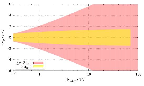
Figure 1: Theoretical uncertainty of the light Higgs mass for a fixed order calculation as function of the SUSY scale. Plot taken from [11].

This has caused significant improvements in the codes: the SUSY particles are now usually decoupled at the SUSY scale with SM RGEs between $M_{Z}$ and $M_{\rm SUSY}$. Moreover, the Higgs mass is not longer calculated at the fixed order but EFT techniques are used:

1. Match the SM and MSSM at $M_{\rm SUSY}$ to obtain $\lambda_{\rm SM}(M_{\rm SUSY})$

2. Run $\lambda_{\rm SM}$ to $m_{t}$

3. Calculate $m_{h}$ at $m_{t}$ with SM corrections

The common models considered as EFT are usually the SM or 2HDMs. An overview about the Tools for the MSSM and their features is given in Tab. 1.

	CPsuperH	FeynHiggs	MhEFT	SoftSUSY	SPheno	Suspect	SusyHD
General
GUT model	✗	✗	✗	✓	✓	✓	✗
CPV	✓	✓	✗	partially	partially	✗	✗
Heavy SUSY
supported	✓	✓	only	-	✓	✗	only
EFT	SM	SM, THDM	THDM	-	SM	-	SM
Other observables
Decays	✓	✓	✓	✓	✓	✓	✗
Flavour	✗	✓	✗	✗	✓	✓	✗
$g-2$	✓	✓	✗	✗	✓	✓	✗
Oblique P.	✗	✓	✗	✗	✓	✗	✗
EDMs	✓	✓	✗	✗	✓	✓	✗

Table 1: Public tools for the MSSM.

2.2 NMSSM

In the NMSSM, The particle content of the MSSM is extended by a gauge singlet superfield $\hat{S}$. The most general, renormalisable and $R$-parity conserving superpotential reads

$${W}_{S}={W}_{\rm{Yukawa}}+\frac{1}{3}\kappa\hat{S}^{3}+{\mu\hat{H}_{u}\hat{H}_{d}}+\lambda\hat{S}\hat{H}_{u}\hat{H}_{d}+{\frac{1}{2}\mu_{s}\hat{S}^{2}+t_{s}\hat{S}}\;,$$ (1)

The dimensionful terms can be forbidden by a $Z_{3}$ symmetry. In general, the scalar sector consists of 3 CP-even and 2 CP-odd states in the CP conserving limit, respectively 5 mixed states. An overview about the available (stand-alone) tools for the NMSSM is given in Tab. 2. One can see that so far no EFT techniques are used in the NMSSM codes, i.e. one should be careful and not use very large SUSY masses.

	NMSSMCalc[12]	NMSSMTools [13]	SoftSUSY[14]
General
No $Z_{3}$	✗	✓	✓
GUT model	✗	✓	✓
CPV	✓	✓	✗
scheme	OS, $\overline{\rm{DR}}$	$\overline{\rm{DR}}$	$\overline{\rm{DR}}$
Heavy SUSY
supported	✗	✗	✗
EFT	-	-	-
Other observables
Decays	✓	✓	✓
Flavour	✗	✓	✗
g-2	✗	✓	✗
Oblique P.	✗	✓	✗
EDMs	✓	✓	✗

Table 2: Public tools for the NMSSM.

3 Non-SUSY Tools

As already mentioned, masses are used as input for non-SUSY tools. Thus, their tasks are a bit different compared to SUSY tools and usually consist of:

• Calculate couplings

• Calculate decays

• Check theoretical constraints: (i) Perturbative unitarity, (ii) Vacuum stability

The reason for checking perturbative unitarity is that randomly chosen masses could correspond to arbitrary large Lagrangian parameters. Therefore, unitarity for 2 $\to$ 2 scattering processes is imposed to filter unphysical points. However, the results very often used in literature are based on crucial assumptions. I’ll discuss this in mode detail in sec. 5.
An overview about the existing tools for non-SUSY models is given in Tab. 3.

	GMcalc [15]	2HDMC[16]	HDECAY extensions [17, 18, 19, 20]
General
Models	Georgi-Machacek	2HDMs	EFT (eHDECAY), SM+Singlet (sHDECAY), 2HDM (C2HDM_HDECAY), N2HDM (N2HDECAY)
Higgs Results
CPV	✗	✗	(✓)
Decays	✓	✓	✓
Theoretical checks
Unitarity	✓	✓	2HDM
Vacuum stability	✓	✓	2HDM
Other Observables
Flavour	✗	✗	✗
Oblique Parameters	✓	✓	2HDM
$g-2$	✓	✓	✗
EDMs	✗	✗	✗

Table 3: Public tools for non-SUSY models.

4 Multipurpose Tools

The idea of multipurpose tools it to generate automatically a numerical tool for the study of a given model. For this purpose, one needs expressions for masses, vertices, RGEs and loop corrections. This is exactly the purpose of the package SARAH[21, 22, 23, 24, 25]: SARAH is a Mathematica package which was developed to get from a minimal input all important properties of SUSY and non-SUSY models:

• all Vertices, Tadpole equations, Masses and Mass matrices

• Two-loop RGEs including the full CP and flavour structure, effects of gauge kinetic mixing, and $R_{\xi}$ dependence of VEVs.

• Loop corrections to masses and precision observables

The necessary input to define a model are the gauge symmetries, particle content, (super)potential, and how the symmetries are broken. SARAH is already delivered with a large variety of SUSY and non-SUSY models. Nowadays, there are two interfaces which make use of the derived information to obtain a spectrum generator:

• The SARAH/SPheno interface

• FlexibelSUSY [26, 27]

	FlexibleSUSY	SPheno
Higgs Results
one-loop	full	full
two-loop	(N)MSSM hardcoded general results in preparation	fully model dependent calculation
Heavy BSM scales
supported	✓	✓
scenarios	several MSSM limits hardcoded	general one-loop matching
Theoretical constraints
Unitarity	✗	✓
Vacuum Stability	✗	via Vevacious
Other Calculations
Decays	in progress	✓
Flavor	✗	✓
$g-2$	✓	✓
EDMs	✓	✓
Oblique P.	($\delta m_{W}$)	✓

Table 4:

The obtained precision for scalar masses is comparable to the dedicated MSSM tools mentioned above. However, for other SUSY models the framework SARAH/SPheno is the only combination which provides important two-loop corrections. In the example for the NMSSM, these are the corrections $(\alpha_{\lambda}+\alpha_{\kappa})^{2}$ for instance. Moreover, with SARAH and SPheno also loop corrected masses for non-SUSY models are available. This becomes important if UV completions of a model are considered: in that case, the input parameters are set at a scale well above the electroweak scale and the calculated masses at the weak scale are no longer an in- but an output, see e.g. [28] for a discussion in the context of 2HDMs.
Until recently, SARAH/SPheno used a fixed order calculation which could be combined with a pole mass matching in the case that all particles but the SM ones are very heavy. This has been improved and an automatised matching between two scalar sectors is now available [29]. This makes it possible to study all kind of mass hierarchies for a given UV model. The hierarchies already implemented in SARAH for the example of the MSSM involving very heavy states are summarised in Fig. 2. With this setup, one could reproduce the results of SusyHD, MhEFT in the respective limits.

Figure 2: Mass hierarchies for the MSSM now implemented in the SARAH/SPheno framework.

5 A few words about unitarity constraints

We had mentioned that most non-SUSY tools check the validity of the underlying Lagrangian parameters. For doing that, they impose constraints on the the $2\to 2$ scattering cross sections: the maximal eigenvalue $|(a^{\rm max}_{0})|$ of the scattering matrix must fulfil

$$(a^{\rm max}_{0})|\leq\frac{1}{2}$$ (2)

Usually, the scattering matrices become huge, e.g. they have dimension $36\times 36$ in 2HDMs and $91\times 91$ in the Georgi-Machacek model. Therefore, very often the approximation is used that all involved masses are much smaller than the scattering energy, i.e.

$$s\gg m_{i}^{2}$$ (3)

The consequence is that only point interactions contribute, while (effective) cubic couplings are completely neglected.
In order to test the validity of this approximation, a full tree-level calculation is now available in SARAH/SPheno taking into also the propagator diagrams [30]. The difference compared the large $s$ approximation can be tremendous as shown in Fig. 3 at the example of a singlet extensions.

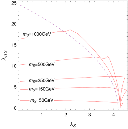
Figure 3: Constraints from perturbative unitarity on the quartic couplings in the singlet extended SM. The purple dashed lines shows the constraint when using the large $s$ approximation, while the red lines show the results from the full calculation. Plot taken from [30].

For scattering energies $s$ close to the masses, we find that the maximal eigenvalue of the scattering matrix is enhanced by a factor

$$\frac{|a^{s}_{0}|}{|a^{s\to\infty}_{0}|}\sim\frac{\lambda_{HS}v^{2}}{m_{h}^{2}}$$ (4)

Thus, the constrains on $\lambda_{HS}$ become stronger up to a factor of 10 for small singlet masses.
The setup was also used to check other models like 2HDMs [31] or triplet extensions [32]. In all cases parameter regions were found, where the large $s$ approximations fails.

6 Summary

Precise predictions for Higgs observables are crucial today. Therefore, many public tools were developed in the past for a fast and accurate study of Higgs properties in BSM models. While the stand-alone numerical tools concentrate on the most widely studied models (MSSM, NMSSM, 2HDMS, GM and SSM), so called ’Spectrum-Generators-Generators’ can be used to go beyond that. These tools create automatically a spectrum generator for a given model which provides very similar features for a large variety of models as the well established tools for the most prominent ones.

References

- [1] B. C. Allanach, Comput. Phys. Commun. 143 (2002) 305 doi:10.1016/S0010-4655(01)00460-X [hep-ph/0104145].
- [2] W. Porod and F. Staub, Comput. Phys. Commun. 183 (2012) 2458 doi:10.1016/j.cpc.2012.05.021 [arXiv:1104.1573 [hep-ph]].
- [3] W. Porod, Comput. Phys. Commun. 153 (2003) 275 doi:10.1016/S0010-4655(03)00222-4 [hep-ph/0301101].
- [4] A. Djouadi, J. L. Kneur and G. Moultaka, Comput. Phys. Commun. 176 (2007) 426 doi:10.1016/j.cpc.2006.11.009 [hep-ph/0211331].
- [5] S. Heinemeyer, W. Hollik and G. Weiglein, Comput. Phys. Commun. 124 (2000) 76 doi:10.1016/S0010-4655(99)00364-1 [hep-ph/9812320].
- [6] J. S. Lee, A. Pilaftsis, M. Carena, S. Y. Choi, M. Drees, J. R. Ellis and C. E. M. Wagner, Comput. Phys. Commun. 156 (2004) 283 doi:10.1016/S0010-4655(03)00463-6 [hep-ph/0307377].
- [7] R. V. Harlander, J. Klappert and A. Voigt, Eur. Phys. J. C 77 (2017) no.12, 814 doi:10.1140/epjc/s10052-017-5368-6 [arXiv:1708.05720 [hep-ph]].
- [8] J. Pardo Vega and G. Villadoro, JHEP 1507 (2015) 159 doi:10.1007/JHEP07(2015)159 [arXiv:1504.05200 [hep-ph]].
- [9] G. Lee and C. E. M. Wagner, Phys. Rev. D 92 (2015) no.7, 075032 doi:10.1103/PhysRevD.92.075032 [arXiv:1508.00576 [hep-ph]].
- [10] D. M. Pierce, J. A. Bagger, K. T. Matchev and R. j. Zhang, Nucl. Phys. B 491 (1997) 3 doi:10.1016/S0550-3213(96)00683-9 [hep-ph/9606211].
- [11] P. Athron, J. h. Park, T. Steudtner, D. Stöckinger and A. Voigt, JHEP 1701 (2017) 079 doi:10.1007/JHEP01(2017)079 [arXiv:1609.00371 [hep-ph]].
- [12] J. Baglio, R. Gröber, M. Mühlleitner, D. T. Nhung, H. Rzehak, M. Spira, J. Streicher and K. Walz, Comput. Phys. Commun. 185 (2014) no.12, 3372 doi:10.1016/j.cpc.2014.08.005 [arXiv:1312.4788 [hep-ph]].
- [13] U. Ellwanger, J. F. Gunion and C. Hugonie, JHEP 0502 (2005) 066 doi:10.1088/1126-6708/2005/02/066 [hep-ph/0406215].
- [14] B. C. Allanach, P. Athron, L. C. Tunstall, A. Voigt and A. G. Williams, Comput. Phys. Commun. 185 (2014) 2322 doi:10.1016/j.cpc.2014.04.015 [arXiv:1311.7659 [hep-ph]].
- [15] K. Hartling, K. Kumar and H. E. Logan, arXiv:1412.7387 [hep-ph].
- [16] D. Eriksson, J. Rathsman and O. Stal, Comput. Phys. Commun. 181 (2010) 189 doi:10.1016/j.cpc.2009.09.011 [arXiv:0902.0851 [hep-ph]].
- [17] R. Contino, M. Ghezzi, C. Grojean, M. Mühlleitner and M. Spira, Comput. Phys. Commun. 185 (2014) 3412 doi:10.1016/j.cpc.2014.06.028 [arXiv:1403.3381 [hep-ph]].
- [18] R. Costa, M. Mühlleitner, M. O. P. Sampaio and R. Santos, JHEP 1606 (2016) 034 doi:10.1007/JHEP06(2016)034 [arXiv:1512.05355 [hep-ph]].
- [19] D. Fontes, M. Mühlleitner, J. C. Romão, R. Santos, J. P. Silva and J. Wittbrodt, JHEP 1802 (2018) 073 doi:10.1007/JHEP02(2018)073 [arXiv:1711.09419 [hep-ph]].
- [20] I. Engeln, M. Mühlleitner and J. Wittbrodt, Comput. Phys. Commun. 234 (2019) 256 doi:10.1016/j.cpc.2018.07.020 [arXiv:1805.00966 [hep-ph]].
- [21] F. Staub, arXiv:0806.0538 [hep-ph].
- [22] F. Staub, Comput. Phys. Commun. 181 (2010) 1077 doi:10.1016/j.cpc.2010.01.011 [arXiv:0909.2863 [hep-ph]].
- [23] F. Staub, Comput. Phys. Commun. 182 (2011) 808 doi:10.1016/j.cpc.2010.11.030 [arXiv:1002.0840 [hep-ph]].
- [24] F. Staub, Comput. Phys. Commun. 184 (2013) 1792 doi:10.1016/j.cpc.2013.02.019 [arXiv:1207.0906 [hep-ph]].
- [25] F. Staub, Comput. Phys. Commun. 185 (2014) 1773 doi:10.1016/j.cpc.2014.02.018 [arXiv:1309.7223 [hep-ph]].
- [26] P. Athron, J. h. Park, D. Stöckinger and A. Voigt, Comput. Phys. Commun. 190 (2015) 139 doi:10.1016/j.cpc.2014.12.020 [arXiv:1406.2319 [hep-ph]].
- [27] P. Athron, M. Bach, D. Harries, T. Kwasnitza, J. h. Park, D. Stöckinger, A. Voigt and J. Ziebell, Comput. Phys. Commun. 230 (2018) 145 doi:10.1016/j.cpc.2018.04.016 [arXiv:1710.03760 [hep-ph]].
- [28] M. E. Krauss, T. Opferkuch and F. Staub, arXiv:1807.07581 [hep-ph].
- [29] M. Gabelmann, M. Mühlleitner and F. Staub, arXiv:1810.12326 [hep-ph].
- [30] M. D. Goodsell and F. Staub, Eur. Phys. J. C 78 (2018) no.8, 649 doi:10.1140/epjc/s10052-018-6127-z [arXiv:1805.07306 [hep-ph]].
- [31] M. D. Goodsell and F. Staub, arXiv:1805.07310 [hep-ph].
- [32] M. E. Krauss and F. Staub, Phys. Rev. D 98 (2018) no.1, 015041 doi:10.1103/PhysRevD.98.015041 [arXiv:1805.07309 [hep-ph]].