Study of Multi-Step Knowledge-Aided Iterative Nested MUSIC for Direction Finding

Abstract

In this work, we propose a subspace-based algorithm for direction-of-arrival (DOA) estimation applied to the signals impinging on a two-level nested array, referred to as multi-step knowledge-aided iterative nested MUSIC method (MS-KAI-Nested-MUSIC), which significantly improves the accuracy of the original Nested-MUSIC. Differently from existing knowledge-aided methods applied to uniform linear arrays (ULAs), which make use of available known DOAs to improve the estimation of the covariance matrix of the input data, the proposed Multi-Step KAI-Nested-MU employs knowledge of the structure of the augmented sample covariance matrix, which is obtained by exploiting the difference co-array structure covariance matrix, and its perturbation terms and the gradual incorporation of prior knowledge, which is obtained on line. The effectiveness of the proposed technique can be noticed by simulations focusing on uncorrelated closely-spaced sources.

I Introduction

Direction-of-arrival (DOA) estimation and beamforming are two main applications of the sensor array. Nevertheless, both of them have been mainly restricted to the case of uniform linear arrays (ULA) [1, 2, 3, 4, 5, 6, 7, 8, 9, 10, 11, 12, 13, 14, 15, 29, 18, 17, 20, 19, 21, 23, 22, 25, 26, 27, 32, 33, 30, 31, 24, 57, 36, 34, 35, 40, 38, 39, 40, 41, 42, 43, 44, 45, 47, 49, 50, 54, 55, 56, 57, 59, 60, 61, 62, 63, 64, 65, 66, 67, 68, 69]. The number of sources that can be resolved with a N element ULA using conventional subspace based methods like MUSIC [70] is N-1. Over the years, the question of detecting more sources than sensors has been dealt with by different means. In [71, 72], the use of minimum redundancy arrays (MRA) [73] and the construction of an enlarged covariance matrix for reaching improved degrees of freedom (DOF) were not successful in making it positive semidefinite for finite number of samples. In [74, 75], an approach to convert the enlarged matrix into an appropriate positive definite Toeplitz matrix was proposed. In spite of that, for achieving more DOF to detect N-1 sources with N sensors, that approach also depends on MRA, for which there is no closed form expression for the array geometry. Moreover, such arrays demand hard designs which are limited to computer simulations or complex algorithms for locating the sensors [76, 77],[78, 79, 80]. In [81], the approach using fourth-order cumulants succeeded in increasing DOF. Yet it is limited to non-Gaussian sources. In [82], by using the Khatri-Rao (KR) product and the hypothesis of quasi-stationary sources, one can recognize 2N-1 sources through a N element ULA without needing to calculate high-order statistics. However, this approach depending on quasi-stationary sources is not appropriate to stationary sources. In [83], the rise of the DOF resulted from building a virtual array making use of a MIMO radar. Since the creation of that array relies on active sensing, that method is not suitable for passive sensing. In [84, 85], by exploring the class of non-uniform arrays, it was suggested an array structure called nested array. It is formed by combining two or more ULAs to obtain a difference co-array, which provides increase of DOF and, therefore, can resolve more sources than the real number of physical sensors. In a subsequent work [86], linear nested arrays were employed to estimate DOAs of distributed sources. Additionally, in [87], it was proposed a robust beamforming for these arrays based on interference-plus-noise reconstruction and steering vector estimation. The four last mentioned studies [84, 85, 86, 87] focus on scenarios composed of multiple unclosely spaced sources in order to assess the performances of their proposed methods in resolving more sources than the real number of physical sensors. For this aim, their signal models assume that the sources are uncorrelated. However, the required vectorization of the initial covariance matrix resulting from the employment of uncorrelated sources already leads to an equivalent source signal vector whose powers of their sources behave like fully coherent ones. For this reason, that method, which is based on a system model assuming uncorrelated sources, makes use of spatial smoothing.

In previous works using ULAs [88, 89, 90, 91], we developed two ESPRIT-based methods known as Two-Step KAI ESPRIT (TS-KAI-ESPRIT), Multi-Step KAI-ESPRIT (MS-KAI-ESPRIT) and the Krylov subspace based Multi-Step KAI-Conjugate Gradient (MS-KAI-CG). All of them make use of the refinements of the covariance matrix estimates via steps of reductions [92, 93] of their undesirable terms. The mentioned methods determine the values of scaling factors that reduce the undesirable terms causing perturbations in the estimates of the signal and noise subspaces in an iterative manner, resulting in better estimates. This is carried out by choosing the set of DOA estimates that have the highest likelihood of being the set of true DOAs. TS-KAI ESPRIT combines this refinement, which has been considered in only two steps, with the use of prior knowledge about signals [94, 95, 96]. Considering a practical scenario, the mentioned previous knowledge could be from the signals coming from known base stations or from static users in a system. The MS-KAI-ESPRIT and MS-KAI-CG, instead of employing prior knowledge about the signals, obtain their initial knowledge on line, i.e. by means of initial estimates, computed at the first step. At each iteration of their second step, the initial Vandermonde matrix is updated by replacing an increasing number of steering vectors of initial estimates with their corresponding newer ones. In other words, at each iteration, the knowledge obtained on line is updated, allowing the correction of the sample covariance matrix estimates, which yields more accurate estimates.

In this work, we propose a subspace-based algorithm for direction-of-arrival (DOA) estimation applied to the signals impinging on a two-level nested array, referred to as multi-step knowledge-aided iterative nested MUSIC method (MS-KAI-Nested-MUSIC), which is inspired by previously reported knowledge-aided techniques. Differently from existing knowledge-aided methods applied to uniform linear arrays (ULAs), which make use of available known DOAs to improve the estimation of the covariance matrix of the input data, the proposed Multi-Step KAI-Nested-MU employs knowledge of the structure of the spatially smoothed covariance matrix, which is obtained from processing part of the difference co-array, its perturbation terms and the gradual incorporation of prior knowledge, which is obtained on line.

The employment of such ULA-based method like MUSIC in a two-level nested array is justified [84] by the following: its difference coarray, in which is based this method, is a filled longer ULA; the spatially-smoothed covariance matrix resulted from processing signals impinging on a two-level nested array is positive semidefinite for any finite number of snapshots; since its resulting smoothed matrix is equal to the square of a covariance matrix obtained from the mentioned longer ULA, both covariance matrices share the same set of eigenvectors and the square of the eigenvalues of the former are equal to the corresponding ones of the later.

This paper is organized as follows. Section II briefly describes the Nested-MUSIC and the necessary background for understanding the proposed technique. Section III presents the proposed MS-KAI-Nested-MUSIC algorithm. Section IV, illustrates and discusses the computational complexity of the proposed algorithm. In Section V, we present the simulation results whereas the conclusions are drawn in Section VI.

Notation: the superscript H denote the Hermitian transposition, $\mathbb{E}[\cdot]$ expresses the expectation operator and $\bm{I}_{M}$ stands for the $M\times M$ identity matrix.

II System Models and Background

II-A The Nested MUSIC system model

Let us consider a two-level nested passive array composed of $\mathit{M}$ sensors, which is a concatenation of two ULAs. The inner ULA has $\mathit{M_{1}}$ sensors with intersensor spacing $\mathit{d}_{1}$ and the outer has $\mathit{M_{2}}$ sensors with intersensor spacing $\mathit{d}_{2}=\left(\mathit{M_{1}}+1\right)\mathit{d}_{1}$. Specifically speaking, it is a linear array with sensors positions obtained by the union of the sets $I_{nner}=\left\{md_{1}\mid\>m=1,2,\ldots,M_{1}\right\}$ and $O_{uter}=\left\{n\left\{M_{1}+1\right\}d_{1}\mid\>n=1,2,\ldots,M_{2}\right\}$. Fig. 1 illustrates a two-level nested array.

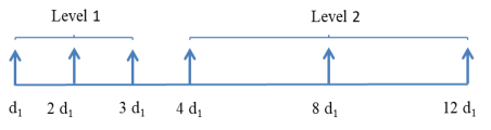
Figure 1: A two level nested array with 3 sensors at each level.

Assuming $\mathit{P}$ uncorrelated narrowband signals from far-field sources at directions $\left\{\theta_{p},p=1,2,\ldots,P\right\}$ impinging on this array, the $i$th data snapshot of the $M$-dimensional array output vector can be modeled as

$$\bm{y}(i)=\bm{F\,s}(i)+\bm{n}(i),\qquad i=1,2,\ldots,N,$$ (1)

where $\bm{y}(i)=[y_{1}(i),y_{2}(i),\ldots,y_{M}(i)]^{T}$ is the received signal vector at the snapshot $\mathit{i}$, $\bm{s}(i)=[s_{1}(i),s_{2}(i),\ldots,s_{P}(i)]^{T}$ is the source signal vector and $s_{p}(i)\sim N^{C}\left(0,\sigma_{k}^{2}\right)$. Additionally, we assume that $\bm{n}(i)=[n_{1}(i),n_{2}(i),\ldots,n_{M}(i)]^{T}$ is the white Gaussian noise vector with power $\sigma_{n}^{2}$ and that its components and the source vector ones are uncorrelated to each other. We also consider that $\bm{f}(\theta_{p})=\left\{e^{-j2\pi\frac{d_{1}}{\lambda_{c}}r_{n}\sin\theta_{p}}\mid n=1,2,\ldots,M\right\}$ denotes the steering vector of the pth signal, where $\lambda_{c}$ stands for the carrier wavelength and

$$\left\{r_{n}\mid n=1,2,\ldots,M\right\}= \left\{0,1,\ldots,M_{1}-1,M_{1},\right.$$

$$\left.2\left(M_{1}+1\right)-1,\ldots,\right.$$

$$\left.M_{2}\left(M_{1}+1\right)-1\right\}$$ (2)

is a vector that contains the location of the sensors. Next, the array manifold containing the steering vectors of the signals can be formed as

$$\bm{F}(\Theta)=[\bm{f}(\theta_{1}),\bm{f}(\theta_{2}),\ldots,\bm{f}(\theta_{P})]$$ (3)

By averaging the N collected snapshots through the time, we can express the sample covariance matrix as

$$\bm{\hat{R}_{1}}=\frac{1}{N}\sum\limits^{N}_{i=1}\bm{y}\left(i\right)\bm{y}^{H}\left(i\right)\approx\mathbb{E}\left[\bm{y}\left(i\right)\bm{y}^{H}\left(i\right)\right]$$

$$=\bm{F}\,\bm{R}_{s}\bm{F}^{H}+\sigma_{n}^{2}\bm{I},$$ (4)

where $\bm{R}_{s}=\mathit{diag}\left\{\sigma_{1}^{2},\sigma_{2}^{2},\ldots,\sigma_{P}^{2}\right\}$

By vectorizing $\bm{\hat{R}_{1}}$ (II-A), we can obtain a long vector, in which some elements appear more than once. By removing these repeated rows and sorting them so that the ith row corresponds to the sensor located at $\left(-\bar{M}+i\right)d_{1}$, where $\bar{M}=\left(M^{2}/4+M/2\right)$, we can obtain a new vector

$$\bm{z}=\bm{G}\>\bm{p}+\sigma_{n}^{2}\bm{e},$$ (5)

where

$$\bm{G}(\Theta)=[\bm{g}(\theta_{1}),\bm{g}(\theta_{2}),\ldots,\bm{g}(\theta_{P})],$$ (6)

in which

$$\bm{g}(\theta_{p})= \left[e^{-j2\pi\frac{d_{1}}{\lambda_{c}}\left(-\bar{M}+1\right)\sin\theta_{p}},e^{-j2\pi\frac{d_{1}}{\lambda_{c}}\left(-\bar{M}+2\right)\sin\theta_{p}},\right.$$

$$\left.\ldots,e^{-j2\pi\frac{d_{1}}{\lambda_{c}}\left(\bar{M}-2\right)\sin\theta_{p}},e^{-j2\pi\frac{d_{1}}{\lambda_{c}}\left(\bar{M}-1\right)\sin\theta_{p}}\right]^{T},$$ (7)

$$\bm{p}=\left[\sigma_{1}^{2},\sigma_{2}^{2},\ldots,\sigma_{P}^{2}\right]^{T},$$ (8)

and

$$\bm{e}\in\mathfrak{R}^{\left(2\bar{M}-1\right)\times 1}$$ (9)

is a vector of all zeros, except for a $\mathit{1}$ at the center position.

By comparing (5) with (1), we can notice that $\bm{z}$ in (5) behaves like the signal received by a longer difference coarray, whose sensors locations can be determined by the distinct values in the set $\left\{r_{i}-r_{j}\mid\>1\leq i,j\leq M\right\}$. The equivalent source signal vector $\bm{p}$ (8) consists of powers $\sigma_{p}^{2}$ of the actual sources and thus they behaves like fully coherent sources[84]. This, combined with the fact that the difference coarray is a filled ULA, motivates to apply spatial smoothing to $\bm{z}$ (5) to obtain a full rank covariance matrix $\widetilde{R}$, as follows:

$$\bm{\widetilde{R}}= \frac{1}{M^{2}/4+M/2}\sum\limits^{M^{2}/4+M/2}_{i=1}\bm{z}_{i}\bm{z}_{i}^{H}$$

$$= \frac{1}{M^{2}/4+M/2}\left(\bm{G}_{1}\bm{R}_{s}\bm{G}_{1}^{H}+\sigma_{n}^{2}\bm{I}\right)^{2},$$ (10)

where $\bm{z}_{i}$ corresponds to the $\left(M^{2}/4+M/2-i+1\right)$ th to $\left(\left(M^{2}-2\right)/2+M-i+1\right)$ th rows of $\bm{z}$ and $\bm{G}_{1}$ is a manifold array composed of the last $\bar{M}$ rows of $\bm{G}$.

It can be shown [84] that the smoothed covariance matrix $\bm{\widetilde{R}}$ (II-A) can be expressed as $\bm{\widetilde{R}}=\bm{\hat{R}}^{2}$, where $\bm{\hat{R}}$ has the same form as the covariance received by a longer ULA composed of $M^{2}/4+M/2$ sensors. Since $\bm{\hat{R}}$ and $\bm{\widetilde{R}}$ share the same set of eigenvectors and the eigenvalues of $\bm{\hat{R}}$ are the square roots of $\bm{\widetilde{R}}$, by eigendecomposition of $\bm{\widetilde{R}}$, we can found the eigenvectors corresponding to the smallest $M^{2}/4+M/2-P$ eigenvalues of $\bm{\hat{R}}$. Due to the previously mentioned reasons and also for being PSD by construction, which results from the sum of vector outer products, the spatially smoothed matrix $\bm{\widetilde{R}}$ can be used as the basis for our proposed MS-KAI-Nested-MUSIC algorithm.

II-B Background - ULA model and MUSIC algorithm

Let us assume that P narrowband signals from far-field sources impinge on a uniform linear array (ULA) of $M_{1}>\textit{P}$ sensor elements from directions ${\bm{\theta}}=[\theta_{1},\theta_{2},\ldots,\theta_{P}]^{T}$. We also consider that the sensors are spaced from each other by a distance $d_{1}\leq\frac{\lambda_{c}}{2}$, where $\lambda_{c}$ is the signal wavelength, and that without loss of generality, we have ${\frac{-\pi}{2}\leq\theta_{1}\leq\theta_{2}\ldots\leq\theta_{P}\leq\frac{\pi}{2}}$.

The $i$th data snapshot of the $M_{1}$-dimensional array output vector can be modeled as

$$\bm{x}\left(i\right)=\bm{A\,s}\left(i\right)+\bm{n}\left(i\right),\qquad i=1,2,\ldots,N,$$ (11)

where $\bm{s}(i)=[s_{1}(i),\ldots,s_{P}(i)]^{T}\in\mathbb{C}^{\mathit{P\times 1}}$ represents the zero-mean source data vector, $\bm{n}(i)\in\mathbb{C}^{\mathit{M_{1}\times 1}}$ is the vector of white circular complex Gaussian noise with zero mean and variance $\sigma_{n}^{2}$, and $N$ denotes the number of available snapshots. The Vandermonde matrix $\bm{A}\left(\Theta\right)=[\bm{a}(\theta_{1}),\ldots,\bm{a}(\theta_{P})]\in\mathbb{C}^{\mathit{M_{1}\times P}}$, known as the array manifold, contains the array steering vectors $\bm{a}(\theta_{j})$ corresponding to the $n$th source, which can be expressed as

$$\bm{a}(\theta_{n})=[1,e^{-j2\pi\frac{d}{\lambda_{c}}\sin\theta_{n}},\ldots,e^{-j2\pi(M_{1}-1)\frac{d}{\lambda_{c}}\sin\theta_{n}}]^{T},$$ (12)

where $n=1,\ldots,P$. Using the fact that $\bm{s}\left(i\right)$ and $\bm{n}\left(i\right)$ are modeled as uncorrelated linearly independent variables, the $M_{1}\times M_{1}$ signal covariance matrix is calculated by

$$\bm{R}=\mathbb{E}\left[\bm{x}\left(i\right)\bm{x}^{H}\left(i\right)\right]=\bm{A}\,\bm{R}_{ss}\bm{A}^{H}+\sigma_{n}^{2}\bm{I}_{M},$$ (13)

where $\bm{R}_{ss}=$ $\mathbb{E}\left[\bm{s}\left(i\right)\bm{s}^{H}\left(i\right)\right]=$ diag $\left\{\sigma_{1}^{2},\sigma_{2}^{2},\ldots,\sigma_{P}^{2}\right\}$. Since the true signal covariance matrix is unknown, it must be estimated and a widely-adopted approach is the sample average formula given by

$$\bm{\hat{R}}=\frac{1}{N}\sum\limits^{N}_{i=1}\bm{x}(i)\bm{x}^{H}(i),$$ (14)

whose estimation accuracy is dependent on $N$.

From [70], it is known that $\bm{R}$ (13) has $M_{1}$ eigenvalues $\left[\lambda_{1},\lambda_{2},\ldots,\lambda_{P}\right]$ and $M_{1}$ associated eigenvectors forming a subspace $\bm{\Phi}=\left[\bm{\phi}_{1},\bm{\phi}_{2},\ldots,\bm{\phi}_{M_{1}}\right]$. By sorting the $M_{1}$ eigenvalues from the smallest to the largest, the subspace $\bm{\Phi}$ can be decomposed into two subspaces $\bm{\Phi}=\left[\bm{\Phi}_{S}\>\bm{\Phi}_{N}\right]$, where $\bm{\Phi}_{S}$ is the $\left[M_{1}\times P\right]$ signal subspace composed of the eigenvectors associated with the impinging signals and $\bm{\Phi}_{N}$ is the $\left[M_{1}\times\left(M_{1}-P\right)\right]$ noise subspace, composed of the eigenvectors associated with the noise. Due to the orthogonality between the noise subspace and the array steering vector at the angles of arrival $\left(\theta_{1},\theta_{2},\ldots,\theta_{P},\right)$, the matrix product $\bm{a}^{H}\left(\theta\right)\bm{\Phi}_{N}\bm{\Phi}_{N}^{H}\bm{a}^{H}\left(\theta\right)$ tends to zero. The reciprocal of this matrix product $\left(\bm{a}^{H}\left(\theta\right)\bm{\Phi}_{N}\bm{\Phi}_{N}^{H}\bm{a}^{H}\left(\theta\right)\right)^{-1}$ called MUSIC pseudospectrum creates sharp peaks at the angles of arrival. By plotting it in the range $\left[-\pi/2\quad\pi/2\right]$, it is possible to determine the peaks and its corresponding angles of arriving by a peak search.

III The proposed MS-KAI-Nested-MUSIC algorithm

The idea behind the MS-KAI-Nested-MUSIC algorithm is to expand the estimated spatially smoothed covariance matrix $\bm{\widetilde{R}}$ (II-A) as if it were generated by the ith data snapshots of $L=M^{2}/4+M/2$-dimensional array output vectors, where, as mentioned in II-A, $M$ is the number of the physical sensors of the nested array. That is to say that we can employ the estimated spatially smoothed covariance matrix $\bm{\widetilde{R}}$ as if it were the estimate provided by the sample average formula. Therefore, after making $\bm{\widetilde{R}}$ (II-A) equal to $\bm{\hat{R}}$ (14) , we can start by expanding the former (II-A) using (11) as follows:

$$\bm{\widetilde{R}}=\frac{1}{N}\sum\limits^{N}_{i=1}(\bm{A}\,s(i)+\bm{n}(i))\>(\bm{A}\,s(i)+\bm{n}(i))^{H}$$

$$=\bm{A}\left\{\frac{1}{N}\sum\limits^{N}_{i=1}\bm{s}(i)\bm{s}^{H}(i)\right\}\bm{A}^{H}+\>\frac{1}{N}\sum\limits^{N}_{i=1}\bm{n}(i)\bm{n}^{H}(i)\;+$$

$$\underbrace{\bm{A}\left\{\frac{1}{N}\sum\limits^{N}_{i=1}\bm{s}(i)\bm{n}^{H}(i)\right\}\>+\>\left\{\frac{1}{N}\sum\limits^{N}_{i=1}\bm{n}(i)\bm{s}^{H}(i)\right\}\bm{A}^{H}}_{\text{"undesirable by-products"}}$$ (15)

The first two terms of $\bm{\widetilde{R}}$ in (15) can be considered as estimates of the two summands of $\bm{R}$ given in (13), which represent the signal and the noise components, respectively. The last two terms in (15) are undesirable by-products, which can be seen as estimates for the correlation between the signal and the noise vectors. The system model under study is based on noise vectors which are zero-mean and also independent of the signal vectors. Thus, the signal and noise components are uncorrelated to each other. As a consequence, for a large enough number of samples $N$, the last two terms pointed out in (15) tend to zero. Nevertheless, in practice the number of available samples can be limited. In such situations, the last two terms in (15) may have significant values, which causes the deviation of the estimates of the signal and the noise subspaces from the true signal and noise ones. The key point of the proposed MS-KAI-Nested-MUSIC algorithm is to modify the smoothed covariance matrix estimate at each iteration by gradually incorporating the knowledge provided by the updated Vandermonde matrices which progressively incorporate the newer estimates from the preceding iteration. Based on these updated Vandermonde matrices, refined estimates of the projection matrices of the signal and noise subspaces are calculated. These estimates of projection matrices associated with the initial smoothed covariance matrix estimate and the reliability factor employed to reduce its by-products allow to choose the set of estimates that has the minimum value of the SMLOF, i.e., the highest likelihood of being the set of the true DOAs. The modified smoothed covariance matrix estimate is computed by deriving a scaled version of the undesirable terms from $\bm{\widetilde{R}},$ which are pointed out in (15).

The steps of the proposed algorithm are listed in Table I. The algorithm starts by computing the spatially smoothed covariance matrix estimate (II-A). Next, based on it, the DOAs are estimated using the original MUSIC [70] algorithm, as briefly described in II-B. The superscript $(\cdot)^{(1)}$ refers to the estimation task performed in the first step. Now, a process composed of $n=1:I$ iterations starts by forming the Vandermonde matrix using the DOA estimates. Then, the amplitudes of the sources are estimated such that the square norm of the differences between the observation vector and the vector containing estimates and the available known DOAs is minimized. This problem can be formulated as

$$\hat{\bm{s}}(i)=\arg\min_{\begin{subarray}{c}\bm{s}\end{subarray}}\parallel\bm{x}(i)-\hat{\bm{A}}\mathbf{s}\parallel^{2}_{2}.$$ (16)

The minimization of (16) is achieved using the least squares technique and the solution is described by

$$\hat{\bm{s}}(i)=(\mathbf{\hat{A}}^{H}\>\mathbf{\hat{A}})^{-1}\>\mathbf{\hat{A}}\>\bm{x}(i)$$ (17)

The noise component is then estimated as the difference between the estimated signal and the observations made by the array, as given by

$$\hat{\bm{n}}(i)=\bm{x}(i)\>-\>\hat{\bm{A}}\>\hat{\bm{s}}(i).$$ (18)

After estimating the signal and noise vectors, the third term in (15) can be computed as

$$\bm{V} \triangleq\hat{\bm{A}}\left\{\frac{1}{N}\sum\limits^{N}_{i=1}\bm{\hat{}}{\mathbf{s}}(i)\bm{\hat{}}{\mathbf{n}}^{H}(i)\right\}$$

$$=\hat{\bm{A}}\left\{\frac{1}{N}\sum\limits^{N}_{i=1}(\mathbf{\hat{A}}^{H}\>\mathbf{\hat{A}})^{-1}\mathbf{\hat{A}}^{H}\bm{x}(i)\right.$$

$$\left.\times(\bm{x}^{H}(i)-\bm{x}^{H}(i)\hat{\mathbf{A}}(\hat{\mathbf{A}}^{H}\hat{\mathbf{A}})^{-1}\>\hat{\mathbf{A}}^{H})\right\}$$

$$=\mathbf{\hat{Q}}_{A}\left\{\frac{1}{N}\sum\limits^{N}_{i=1}\bm{x}(i)\bm{x}^{H}(i)\>\left(\mathbf{I}_{M}\>-\>\hat{\mathbf{Q}}_{A}\right)\right\}$$

$$=\mathbf{\hat{Q}}_{A}\>\mathbf{\widetilde{R}}\>\mathbf{\hat{Q}}_{A}^{\perp},$$ (19)

where

$$\mathbf{\hat{Q}}_{A}\triangleq\mathbf{\hat{A}}\>(\mathbf{\hat{A}}^{H}\>\mathbf{\hat{A}})^{-1}\>\mathbf{\hat{A}}^{H}$$ (20)

is an estimate of the projection matrix of the signal subspace, and

$$\mathbf{\hat{Q}}_{A}^{\perp}\triangleq\mathbf{I}_{M}\>-\>\mathbf{\hat{Q}}_{A}$$ (21)

is an estimate of the projection matrix of the noise subspace.

Next, as part of the process of $n=1:I$ iterations, the modified data covariance matrix $\mathbf{\widetilde{R}}^{(n+1)}$ is calculated by computing a scaled version of the estimated terms from the initial smoothed covariance matrix as given

$$\mathbf{\widetilde{R}}^{(n+1)}=\mathbf{\widetilde{R}}\>-\>\mathrm{\mu}\>(\mathbf{V}^{(n)}\>+\>\mathbf{V}^{(n)H}),$$ (22)

where the superscript $(\cdot)^{(n)}$ refers to the $n^{th}$ iteration performed. The scaling or reliability factor $\mu$ increases from 0 to 1 incrementally, resulting in modified smoothed covariance matrix estimates. Each of them gives origin to new estimated DOAs also denoted by the superscript $(\cdot)^{(n+1)}$ by using the MUSIC algorithm, as briefly described in II-B.

In this work, the rank P is assumed to be known, which is an assumption frequently found in the literature. Alternatively, the rank P could be estimated by model-order selection schemes [97] such as Akaike’s Information Theoretic Criterion (AIC) [98] and the Minimum Descriptive Length (MDL) Criterion [99].

Then, a new Vandermonde matrix $\mathbf{\hat{B}}^{(n+1)}$ is formed by the steering vectors of those newer estimated DOAs. By using this new matrix, it is possible to compute the newer estimates of the projection matrices of the signal $\mathbf{\hat{Q}}_{B}^{(n+1)}$ and the noise $\mathbf{\hat{Q}}_{B}^{(n+1)\perp}$ subspaces.

Afterwards, employing the newer estimates of the projection matrices, the initial smoothed covariance matrix estimate, $\bm{\hat{R}}$, the number of its corresponding sensors and the number of sources, the stochastic maximum likelihood objective function $\mathit{U^{(n+1)}(\mu)}$ [100] is computed for each value of $\mu$ at the $n^{th}$ iteration, as follows:

$$\mathit{U^{(n+1)}(\mu)}=\mathrm{ln\>det}\left(\cdot\right),$$ (23)

where

$$\left(\cdot\right)=\left(\mathbf{\hat{Q}}_{B}^{(n+1)}\>\mathbf{\widetilde{R}}\>\mathbf{\hat{Q}}_{B}^{(n+1)}+\dfrac{{\rm Trace}\{\mathbf{\hat{Q}}_{B}^{\perp\>(n+1)}\>\mathbf{\widetilde{R}}\}}{\mathrm{L-P}}\>\mathbf{\hat{Q}}_{B}^{\>(n+1)\perp}\right)$$

The preceding computation selects the set of unavailable DOA estimates that have a higher likelihood at each iteration. Then, the set of estimated DOAs corresponding to the optimum value of $\mu$ that minimizes (23) also at each $n^{th}$ iteration is determined. Finally, the output of the proposed MS-KAI-Nested-MUSIC algorithm is formed by the set of the estimates obtained at the $I^{th}$ iteration, as described in Table I.

TABLE I: MS-KAI-Nested-MUSIC algorithm

Inputs:

$\mathit{M_{1}}$,  $\mathit{M_{2}}$,  $\mathit{d}$,  $\lambda$,  $\mathit{N}$,  $\mathit{P}$

Received vectors $\bm{y}\left(1\right)$,  $\bm{y}\left(2\right)$,$\cdots$, $\bm{y}\left(N\right)$

Outputs:

Estimates $\mathit{\hat{\theta}_{1}^{(n+1)}(\mu\,opt)}$,  $\mathit{\hat{\theta}_{2}^{(n+1)}(\mu\,opt)}$,$\cdots$,  $\mathit{\hat{\theta}_{P}^{(n+1)}(\mu\,opt)}$

First step:

$\{\mathit{\hat{\theta}_{1}}^{(1)},\>\mathit{\hat{\theta}_{2}}^{(1)},\cdots,\mathit{\hat{\theta}_{P}}^{(1)}\}\;\;\underleftarrow{MUSIC}$ $\>(\bm{\widetilde{R}},P,d,\lambda)$

$\bm{\hat{A}}^{(1)}=\left[\bm{a}(\mathit{\hat{\theta}_{1}^{(1)}}),\bm{a}(\mathit{\hat{\theta}_{2}^{(1)}}),\cdots,\bm{a}(\mathit{\hat{\theta}_{P}^{(1)}})\right]$

Second step:

for n =  1 : I

$\bm{\hat{Q}}_{A}^{(n)}=\bm{\hat{A}}^{(n)}\>(\bm{\hat{A}}^{(n)H}\>\bm{\hat{A}}^{(n)})^{-1}\>\bm{\hat{A}}^{(n)H}$

$\bm{\hat{Q}}_{A}^{(n)\perp}=\bm{I}_{M}\>-\>\bm{\hat{Q}}_{A}^{(n)}$

$\bm{V}^{(n)}=\bm{\hat{Q}}_{A}^{(n)}\>\bm{\widetilde{R}}\>\bm{\hat{Q}}_{A}^{(n)\perp}$

for $\bm{\mu}=\mathrm{\>0:\iota\>:1}$

$\bm{\widetilde{R}}^{(n+1)}=\bm{\widetilde{R}}\>-\>\mathrm{\mu}\>(\bm{V}^{(n)}\>+\>\bm{V}^{(n)H})$

$\{\mathit{\hat{\theta}_{1}}^{(n+1)},\>\mathit{\hat{\theta}_{2}}^{(n+1)},\cdots,\mathit{\hat{\theta}_{P}}^{(n+1)}\}\;\;\underleftarrow{MUSIC}$ $\>(\bm{\widetilde{R}}^{(n+1)},\>P,d,\lambda)$

$\bm{\hat{B}}^{(n+1)}=\left[\bm{a}(\mathit{\hat{\theta}_{1}^{(n+1)}}),\bm{a}(\mathit{\hat{\theta}_{2}^{(n+1)}}),\cdots,\bm{a}(\mathit{\hat{\theta}_{P}^{(n+1)}})\right]$

$\bm{\hat{Q}}_{B}^{(n+1)}=\bm{\hat{B}}^{(n+1)}\>(\bm{\hat{B}}^{(n+1)H}\>\bm{\hat{B}}^{(n+1)})^{-1}\>\bm{\hat{B}}^{(n+1)H}$

$\bm{\hat{Q}}_{B}^{(n+1)\perp}=\bm{I}_{M}\>-\>\bm{\hat{Q}}_{B}^{(n+1)}$

$\mathit{U^{(n+1)}(\mu)}=\mathrm{ln\>det}\left(\cdot\right),$

$\left(\cdot\right)=\left(\bm{\hat{Q}}_{B}^{(n+1)}\>\bm{\widetilde{R}}\>\bm{\hat{Q}}_{B}^{(n+1)}+\dfrac{{\rm Trace}\{\bm{\hat{Q}}_{B}^{\perp\>(n+1)}\>\bm{\widetilde{R}}\}}{\mathit{L-P}}\>\bm{\hat{Q}}_{B}^{\>(n+1)\perp}\right)$

$\mathit{\mu}_{\mathrm{o}}^{(n+1)}=\arg\min\hskip 2.84526pt\mathit{U^{(n+1)}(\mu)}$

$\mathrm{DOAs}^{(n+1)}=\left(\ast\right),$

$\left(\ast\right)=\{\mathit{\hat{\theta}_{1}^{(n+1)}(\mu_{o})}$,  $\mathit{\hat{\theta}_{2}^{(n+1)}(\mu_{o})}$,$\cdots$,  $\mathit{\hat{\theta}_{P}^{(n+1)}(\mu_{o})}\}$

$\textbf{if}\hskip 2.84526pt\mathit{n<=\;P}$

$\bm{\hat{A}}^{(n+1)}=\left\{\bm{a}(\mathit{\hat{\theta}_{\{1,\cdots,n\}}^{(n+1)}(\mu_{o})})\right\}\bigcup\left\{\bm{a}(\mathit{\hat{\theta}_{\{1,\cdots,P\}\,-\,\{1,\cdots,n\}}^{(1)}})\right\}$

else

$\bm{\hat{A}}^{(n+1)}=\left(\ast\right),$

$\left(\ast\right)=\left[\bm{a}(\mathit{\hat{\theta}_{1}^{(n+1)}}(\mu_{o})),\bm{a}(\mathit{\hat{\theta}_{2}^{(n+1)}}(\mu_{o})),\cdots,\bm{a}(\mathit{\hat{\theta}_{P}^{(n+1)}}(\mu_{o}))\right]$

end if

end for

end for

IV Computational Complexity Analysis

In this section, we evaluate the approximate computational cost of the proposed MS-KAI-Nested-MUSIC algorithm in terms of multiplications and additions. For this purpose, we make use of Table II, where $\mathrm{\tau}=\frac{1}{\iota}+1$. The increment ${\iota}$ is defined in Table I. From Table II, it can be seen that assuming the specific configuration used in the simulations V, MS-KAI-Nested-MUSIC shows a roughly similar computational burden in terms of multiplications and also of additions with

$\mathcal{O}\left\{I\tau\left[\frac{180}{\Delta}\left(\frac{M^{2}}{4}+\frac{M}{2}\right)^{2}\right]+\left(\frac{M^{2}}{4}+\frac{M}{2}\right)8N^{2}\right\}$, where $\tau$ is typically an integer that ranges from $1$ to $20$, $\Delta$ stands for the search step and $I$ is the number of iterations at the $2nd$ step. The relatively high costs come from the two nested loops for computing $I\times\tau$ times two subprocesses at its second step. These nested loops, from which the last is the more significant, concentrate most of the required operations. For this reason it is responsible for most of the burden of the proposed MS-KAI-Nested-MUSIC algorithm.

TABLE II: MS-KAI-Nested-MUSIC algorithm

Multiplications

$\approx\>I\tau\left\{\frac{180}{\Delta}[\left(\frac{M^{2}}{4}+\frac{M}{2}\right)^{2}+\left(\frac{M^{2}}{4}+\frac{M}{2}\right)\left(2-P\right)-P]\right.$

$\left.+\left(\frac{M^{2}}{4}+\frac{M}{2}\right)8N^{2}{+\frac{10}{3}\left(\frac{M^{2}}{4}+\frac{M}{2}\right)^{3}}+\left(\frac{M^{2}}{4}+\frac{M}{2}\right)^{2}\left(P+2\right)\right.$

$\left.+\left(\frac{M^{2}}{4}+\frac{M}{2}\right)\left(P^{2}+2P\right)+\frac{P^{3}}{2}+\frac{3P^{2}}{2}\right\}$

Additions

$\approx\>I\tau\left\{\frac{180}{\Delta}[\left(\frac{M^{2}}{4}+\frac{M}{2}\right)^{2}-\left(\frac{M^{2}}{4}+\frac{M}{2}\right)\left(P-1\right)]\right.$

$\left.+\left(\frac{M^{2}}{4}+\frac{M}{2}\right)8N^{2}{+\frac{10}{3}\left(\frac{M^{2}}{4}+\frac{M}{2}\right)^{3}}+\left(\frac{M^{2}}{4}+\frac{M}{2}\right)^{2}\left(P-1\right)\right.$

$\left.+\left(\frac{M^{2}}{4}+\frac{M}{2}\right)\left(\frac{3P^{2}}{2}+\frac{5P}{2}-1\right)-P^{2}-\frac{P}{2}\right\}$

V Simulations

In this section, we examine the performance of the proposed MS-KAI-Nested-MUSIC algorithm in terms of probability of resolution (PR) and RMSE and compare them to the corresponding performances of Nested-MUSIC [84] and of the original MUSIC [70]. We focus on the specific case of closely-spaced sources.

We employ $M=8$ sensors in the algorithms based on two-level nested array and, in the original MUSIC, we use a ULA with $M_{1}=20$ sensors, which is also the same number of sensors $\left(M^{2}/4+M/2\right)$ of the filled ULA obtained from part of the difference coarray, which is the actual number of sensors employed the Nested-MUSIC and MS-KAI-Nested-MUSIC algorithms. We assume an inter-element spacing $\Delta=\frac{\lambda_{c}}{2}$ and also that there are two uncorrelated complex Gaussian signals with equal power impinging on the arrays. The closely-spaced sources are separated by $2^{o}$, at $\mathrm{(}15^{o},17^{o})$. The first two figures make use of $N=150$ snapshots and $L_{r}=250$ trials, whereas the two later ones employ $3.33dB$ and $L_{r}=250$ trials.

In Fig. 4, we show the probability of resolution versus SNR. We take into account the criterion [101], in which two sources with DOAs $\theta_{1}$ and $\theta_{2}$ are said to be resolved if their respective estimates $\hat{\theta}_{1}$ and $\hat{\theta}_{2}$ are such that both $\left|\hat{\theta}_{1}-\theta_{1}\right|$ and $\left|\hat{\theta}_{2}-\theta_{2}\right|$ are less than $\left|\theta_{1}-\theta_{2}\right|/2$. It can be seen the superior performance of the proposed MS-KAI-Nested-MUSIC in the range $\left(-10\;7\right)dB$. From this point on, all considered algorithms provide similar performance. The gap between the proposed MS-KAI-Nested-MUSIC and the Nested-MUSIC [84] shows a significant improvement achieved in terms of PR. It can be noticed a bigger gap between the proposed MS-KAI-Nested-MUSIC and the original MUSIC [70], whose number of physical sensors is $2.5\times$ the number of the physical sensors of the other two-level nested based algorithms under comparison, what means an important saving of sensors.

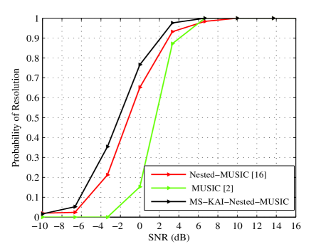
Figure 2: Probability of resolution versus SNR with $P=2$, $M=8$, $N=150$, $L_{r}=250$ runs

In Fig. 3, it is shown the RMSE in degrees versus SNR. The RMSE is defined as

$$\centering\mathrm{RMSE}=\sqrt{\frac{1}{L_{r}\>P}\sum\limits^{L_{r}}_{l=1}\sum\limits^{P}_{p=1}\bm{(}\theta_{p}-\bm{\hat{}}{\theta}_{p}(l))^{2}},\@add@centering$$ (24)

where $L_{r}$ is the number of trials.

It can be noticed that the MS-KAI-Nested-MUSIC outperforms Nested-MUSIC, in the whole range under consideration. In the range $\left[-10\;-1.8\right)dB$., it is outperformed by conventional MUSIC, however, the achieved levels of RMSE are still. From $-1.8$ to $6.7\,dB$ MS-KAI-Nested-MUSIC is superior to it. From $10\,dB$ on all algorithms have similar performance. As mentioned before, it must be highlighted that in this specific case MUSIC makes use of a ULA whose number of physical sensors is $2.5\times$ the number of the physical sensors of the other two-level nested based algorithms under comparison.

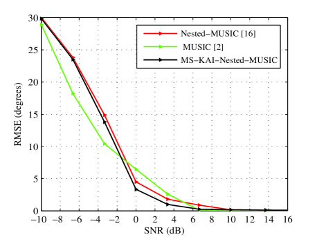
Figure 3: RMSE in degrees versus SNR with with $P=2$, $M=8$, $N=150$, $L_{r}=250$ runs.

In Fig. 4, it is shown the influence of the number of snapshots on the probability of resolution. For this purpose we have set the SNR at $3.33\,dB$ and employed $500$ trials. From the curves, it can be noticed the superior performance in the range $\left[25\;250\right)$ snapshots. From this upper bound on, all algorithms have the same performance.

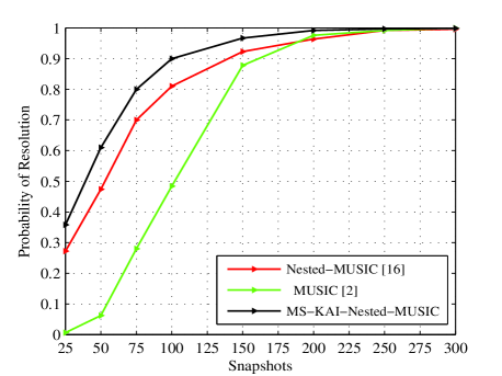
Figure 4: Probability of resolution versus SNR with $P=2$, $M=8$, $SNR=3.33\,dB$, $L_{r}=500$ runs.

In Fig. 5, it is shown the influence of the number of snapshots on RMSE. In this case, we also set the SNR at $3.33\,dB$ and employed $500$ trials. It can be seen that the performance of the MS-KAI-Nested-MUSIC is superior to the Nested-MUSIC. It can also be noticed that except for the range $\left[25\;50\right)$, in which the RMSE has high levels, the performance of MS-KAI-Nested-MUSIC is also superior to the the original MUSIC [70], whose number of physical sensors is $2.5\times$ the number of the physical sensors of the other two-level nested based algorithms under comparison.

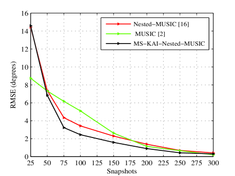
Figure 5: RMSE versus SNR with $P=2$, $M=8$, $SNR=3.33\,dB$, $L_{r}=500$ runs.

VI Conclusions

We have proposed the MS-KAI-Nested-MUSIC algorithm which gradually exploits the knowledge of source signals obtained on line and the structure of the covariance matrix and its perturbations. MS-KAI-Nested-MUSIC algorithm can obtain significant gains in RMSE or probability of resolution performance over the original Nested-MUSIC, and has excellent potential for applications with sufficiently large data records in large-scale antenna systems for wireless communications, radar and other large sensor arrays.

References

- [1] Van Trees, H. L.: ’Optimum Array Processing’, (Wiley,New York, 2002).
- [2] H. Ruan and R. C. de Lamare, “Robust Adaptive Beamforming Using a Low-Complexity Shrinkage-Based Mismatch Estimation Algorithm,” IEEE Sig. Proc. Letters., Vol. 21, No. 1, pp 60-64, 2013.
- [3] A. Elnashar, “Efficient implementation of robust adaptive beamforming based on worst-case performance optimization,” IET Signal Process., Vol. 2, No. 4, pp. 381-393, Dec 2008.
- [4] J. Zhuang and A. Manikas, “Interference cancellation beamforming robust to pointing errors,” IET Signal Process., Vol. 7, No. 2, pp. 120-127, April 2013.
- [5] L. Wang and R. C. de Lamare, “Constrained adaptive filtering algorithms based on conjugate gradient techniques for beamforming,” IET Signal Process., Vol. 4, No. 6, pp. 686-697, Feb 2010.
- [6] H. Ruan and R. C. de Lamare, ”Robust Adaptive Beamforming Based on Low-Rank and Cross-Correlation Techniques,” in IEEE Transactions on Signal Processing, vol. 64, no. 15, pp. 3919-3932, 1 Aug.1, 2016.
- [7] H. Ruan and R. C. de Lamare, “Low-Complexity Robust Adaptive Beamforming Based on Shrinkage and Cross-Correlation,” 19th International ITG Workshop on Smart Antennas, pp 1-5, March 2015.
- [8] L. L. Scharf and D. W. Tufts, “Rank reduction for modeling stationary signals,” IEEE Transactions on Acoustics, Speech and Signal Processing, vol. ASSP-35, pp. 350-355, March 1987.
- [9] A. M. Haimovich and Y. Bar-Ness, “An eigenanalysis interference canceler,” IEEE Trans. on Signal Processing, vol. 39, pp. 76-84, Jan. 1991.
- [10] D. A. Pados and S. N. Batalama ”Joint space-time auxiliary vector filtering for DS/CDMA systems with antenna arrays” IEEE Transactions on Communications, vol. 47, no. 9, pp. 1406 - 1415, 1999.
- [11] J. S. Goldstein, I. S. Reed and L. L. Scharf ”A multistage representation of the Wiener filter based on orthogonal projections” IEEE Transactions on Information Theory, vol. 44, no. 7, 1998.
- [12] Y. Hua, M. Nikpour and P. Stoica, ”Optimal reduced rank estimation and filtering,” IEEE Transactions on Signal Processing, pp. 457-469, Vol. 49, No. 3, March 2001.
- [13] M. L. Honig and J. S. Goldstein, “Adaptive reduced-rank interference suppression based on the multistage Wiener filter,” IEEE Transactions on Communications, vol. 50, no. 6, June 2002.
- [14] E. L. Santos and M. D. Zoltowski, “On Low Rank MVDR Beamforming using the Conjugate Gradient Algorithm”, Proc. IEEE International Conference on Acoustics, Speech and Signal Processing, 2004.
- [15] Q. Haoli and S.N. Batalama, “Data record-based criteria for the selection of an auxiliary vector estimator of the MMSE/MVDR filter”, IEEE Transactions on Communications, vol. 51, no. 10, Oct. 2003, pp. 1700 - 1708.
- [16] R. C. de Lamare and R. Sampaio-Neto, “Reduced-Rank Adaptive Filtering Based on Joint Iterative Optimization of Adaptive Filters”, IEEE Signal Processing Letters, Vol. 14, no. 12, December 2007.
- [17] Z. Xu and M.K. Tsatsanis, “Blind adaptive algorithms for minimum variance CDMA receivers,” IEEE Trans. Communications, vol. 49, No. 1, January 2001.
- [18] R. C. de Lamare and R. Sampaio-Neto, “Low-Complexity Variable Step-Size Mechanisms for Stochastic Gradient Algorithms in Minimum Variance CDMA Receivers”, IEEE Trans. Signal Processing, vol. 54, pp. 2302 - 2317, June 2006.
- [19] C. Xu, G. Feng and K. S. Kwak, “A Modified Constrained Constant Modulus Approach to Blind Adaptive Multiuser Detection,” IEEE Trans. Communications, vol. 49, No. 9, 2001.
- [20] Z. Xu and P. Liu, “Code-Constrained Blind Detection of CDMA Signals in Multipath Channels,” IEEE Sig. Proc. Letters, vol. 9, No. 12, December 2002.
- [21] R. C. de Lamare and R. Sampaio Neto, ”Blind Adaptive Code-Constrained Constant Modulus Algorithms for CDMA Interference Suppression in Multipath Channels”, IEEE Communications Letters, vol 9. no. 4, April, 2005.
- [22] L. Landau, R. C. de Lamare and M. Haardt, “Robust adaptive beamforming algorithms using the constrained constant modulus criterion,” IET Signal Processing, vol.8, no.5, pp.447-457, July 2014.
- [23] R. C. de Lamare, “Adaptive Reduced-Rank LCMV Beamforming Algorithms Based on Joint Iterative Optimisation of Filters”, Electronics Letters, vol. 44, no. 9, 2008.
- [24] R. C. de Lamare and R. Sampaio-Neto, “Adaptive Reduced-Rank Processing Based on Joint and Iterative Interpolation, Decimation and Filtering”, IEEE Transactions on Signal Processing, vol. 57, no. 7, July 2009, pp. 2503 - 2514.
- [25] R. C. de Lamare and Raimundo Sampaio-Neto, “Reduced-rank Interference Suppression for DS-CDMA based on Interpolated FIR Filters”, IEEE Communications Letters, vol. 9, no. 3, March 2005.
- [26] R. C. de Lamare and R. Sampaio-Neto, “Adaptive Reduced-Rank MMSE Filtering with Interpolated FIR Filters and Adaptive Interpolators”, IEEE Signal Processing Letters, vol. 12, no. 3, March, 2005.
- [27] R. C. de Lamare and R. Sampaio-Neto, “Adaptive Interference Suppression for DS-CDMA Systems based on Interpolated FIR Filters with Adaptive Interpolators in Multipath Channels”, IEEE Trans. Vehicular Technology, Vol. 56, no. 6, September 2007.
- [28] R. C. de Lamare, “Adaptive Reduced-Rank LCMV Beamforming Algorithms Based on Joint Iterative Optimisation of Filters,” Electronics Letters, 2008.
- [29] R. C. de Lamare and R. Sampaio-Neto, “Reduced-rank adaptive filtering based on joint iterative optimization of adaptive filters”, IEEE Signal Process. Lett., vol. 14, no. 12, pp. 980-983, Dec. 2007.
- [30] R. C. de Lamare, M. Haardt, and R. Sampaio-Neto, “Blind Adaptive Constrained Reduced-Rank Parameter Estimation based on Constant Modulus Design for CDMA Interference Suppression”, IEEE Transactions on Signal Processing, June 2008.
- [31] M. Yukawa, R. C. de Lamare and R. Sampaio-Neto, “Efficient Acoustic Echo Cancellation With Reduced-Rank Adaptive Filtering Based on Selective Decimation and Adaptive Interpolation,” IEEE Transactions on Audio, Speech, and Language Processing, vol.16, no. 4, pp. 696-710, May 2008.
- [32] R. C. de Lamare and R. Sampaio-Neto, “Reduced-rank space-time adaptive interference suppression with joint iterative least squares algorithms for spread-spectrum systems,” IEEE Trans. Vehi. Technol., vol. 59, no. 3, pp. 1217-1228, Mar. 2010.
- [33] R. C. de Lamare and R. Sampaio-Neto, “Adaptive reduced-rank equalization algorithms based on alternating optimization design techniques for MIMO systems,” IEEE Trans. Vehi. Technol., vol. 60, no. 6, pp. 2482-2494, Jul. 2011.
- [34] R. C. de Lamare, L. Wang, and R. Fa, “Adaptive reduced-rank LCMV beamforming algorithms based on joint iterative optimization of filters: Design and analysis,” Signal Processing, vol. 90, no. 2, pp. 640-652, Feb. 2010.
- [35] R. Fa, R. C. de Lamare, and L. Wang, “Reduced-Rank STAP Schemes for Airborne Radar Based on Switched Joint Interpolation, Decimation and Filtering Algorithm,” IEEE Transactions on Signal Processing, vol.58, no.8, Aug. 2010, pp.4182-4194.
- [36] L. Wang and R. C. de Lamare, ”Low-Complexity Adaptive Step Size Constrained Constant Modulus SG Algorithms for Blind Adaptive Beamforming”, Signal Processing, vol. 89, no. 12, December 2009, pp. 2503-2513.
- [37] L. Wang and R. C. de Lamare, “Adaptive Constrained Constant Modulus Algorithm Based on Auxiliary Vector Filtering for Beamforming,” IEEE Transactions on Signal Processing, vol. 58, no. 10, pp. 5408-5413, Oct. 2010.
- [38] L. Wang, R. C. de Lamare, M. Yukawa, ”Adaptive Reduced-Rank Constrained Constant Modulus Algorithms Based on Joint Iterative Optimization of Filters for Beamforming,” IEEE Transactions on Signal Processing, vol.58, no.6, June 2010, pp.2983-2997.
- [39] L. Wang, R. C. de Lamare and M. Yukawa, “Adaptive reduced-rank constrained constant modulus algorithms based on joint iterative optimization of filters for beamforming”, IEEE Transactions on Signal Processing, vol.58, no. 6, pp. 2983-2997, June 2010.
- [40] L. Wang and R. C. de Lamare, “Adaptive constrained constant modulus algorithm based on auxiliary vector filtering for beamforming”, IEEE Transactions on Signal Processing, vol. 58, no. 10, pp. 5408-5413, October 2010.
- [41] R. Fa and R. C. de Lamare, “Reduced-Rank STAP Algorithms using Joint Iterative Optimization of Filters,” IEEE Transactions on Aerospace and Electronic Systems, vol.47, no.3, pp.1668-1684, July 2011.
- [42] Z. Yang, R. C. de Lamare and X. Li, “L1-Regularized STAP Algorithms With a Generalized Sidelobe Canceler Architecture for Airborne Radar,” IEEE Transactions on Signal Processing, vol.60, no.2, pp.674-686, Feb. 2012.
- [43] Z. Yang, R. C. de Lamare and X. Li, “Sparsity-aware space–time adaptive processing algorithms with L1-norm regularisation for airborne radar”, IET signal processing, vol. 6, no. 5, pp. 413-423, 2012.
- [44] Neto, F.G.A.; Nascimento, V.H.; Zakharov, Y.V.; de Lamare, R.C., ”Adaptive re-weighting homotopy for sparse beamforming,” in Signal Processing Conference (EUSIPCO), 2014 Proceedings of the 22nd European , vol., no., pp.1287-1291, 1-5 Sept. 2014
- [45] Almeida Neto, F.G.; de Lamare, R.C.; Nascimento, V.H.; Zakharov, Y.V.,“Adaptive reweighting homotopy algorithms applied to beamforming,” IEEE Transactions on Aerospace and Electronic Systems, vol.51, no.3, pp.1902-1915, July 2015.
- [46] L. Wang, R. C. de Lamare and M. Haardt, “Direction finding algorithms based on joint iterative subspace optimization,” IEEE Transactions on Aerospace and Electronic Systems, vol.50, no.4, pp.2541-2553, October 2014.
- [47] S. D. Somasundaram, N. H. Parsons, P. Li and R. C. de Lamare, “Reduced-dimension robust capon beamforming using Krylov-subspace techniques,” IEEE Transactions on Aerospace and Electronic Systems, vol.51, no.1, pp.270-289, January 2015.
- [48] S. Xu and R.C de Lamare, , Distributed conjugate gradient strategies for distributed estimation over sensor networks, Sensor Signal Processing for Defense SSPD, September 2012.
- [49] S. Xu, R. C. de Lamare, H. V. Poor, “Distributed Estimation Over Sensor Networks Based on Distributed Conjugate Gradient Strategies”, IET Signal Processing, 2016 (to appear).
- [50] S. Xu, R. C. de Lamare and H. V. Poor, Distributed Compressed Estimation Based on Compressive Sensing, IEEE Signal Processing letters, vol. 22, no. 9, September 2014.
- [51] S. Xu, R. C. de Lamare and H. V. Poor, “Distributed reduced-rank estimation based on joint iterative optimization in sensor networks,” in Proceedings of the 22nd European Signal Processing Conference (EUSIPCO), pp.2360-2364, 1-5, Sept. 2014
- [52] S. Xu, R. C. de Lamare and H. V. Poor, “Adaptive link selection strategies for distributed estimation in diffusion wireless networks,” in Proc. IEEE International Conference onAcoustics, Speech and Signal Processing (ICASSP), , vol., no., pp.5402-5405, 26-31 May 2013.
- [53] S. Xu, R. C. de Lamare and H. V. Poor, “Dynamic topology adaptation for distributed estimation in smart grids,” in Computational Advances in Multi-Sensor Adaptive Processing (CAMSAP), 2013 IEEE 5th International Workshop on , vol., no., pp.420-423, 15-18 Dec. 2013.
- [54] S. Xu, R. C. de Lamare and H. V. Poor, “Adaptive Link Selection Algorithms for Distributed Estimation”, EURASIP Journal on Advances in Signal Processing, 2015.
- [55] N. Song, R. C. de Lamare, M. Haardt, and M. Wolf, “Adaptive Widely Linear Reduced-Rank Interference Suppression based on the Multi-Stage Wiener Filter,” IEEE Transactions on Signal Processing, vol. 60, no. 8, 2012.
- [56] N. Song, W. U. Alokozai, R. C. de Lamare and M. Haardt, “Adaptive Widely Linear Reduced-Rank Beamforming Based on Joint Iterative Optimization,” IEEE Signal Processing Letters, vol.21, no.3, pp. 265-269, March 2014.
- [57] R.C. de Lamare, R. Sampaio-Neto and M. Haardt, ”Blind Adaptive Constrained Constant-Modulus Reduced-Rank Interference Suppression Algorithms Based on Interpolation and Switched Decimation,” IEEE Trans. on Signal Processing, vol.59, no.2, pp.681-695, Feb. 2011.
- [58] Y. Cai, R. C. de Lamare, “Adaptive Linear Minimum BER Reduced-Rank Interference Suppression Algorithms Based on Joint and Iterative Optimization of Filters,” IEEE Communications Letters, vol.17, no.4, pp.633-636, April 2013.
- [59] R. C. de Lamare and R. Sampaio-Neto, “Sparsity-Aware Adaptive Algorithms Based on Alternating Optimization and Shrinkage,” IEEE Signal Processing Letters, vol.21, no.2, pp.225,229, Feb. 2014.
- [60] R. C. de Lamare, “Massive MIMO Systems: Signal Processing Challenges and Future Trends”, Radio Science Bulletin, December 2013.
- [61] W. Zhang, H. Ren, C. Pan, M. Chen, R. C. de Lamare, B. Du and J. Dai, “Large-Scale Antenna Systems With UL/DL Hardware Mismatch: Achievable Rates Analysis and Calibration”, IEEE Trans. Commun., vol.63, no.4, pp. 1216-1229, April 2015.
- [62] R. C. De Lamare and R. Sampaio-Neto, ”Minimum Mean-Squared Error Iterative Successive Parallel Arbitrated Decision Feedback Detectors for DS-CDMA Systems,” in IEEE Transactions on Communications, vol. 56, no. 5, pp. 778-789, May 2008.
- [63] R. C. de Lamare, ”Adaptive and Iterative Multi-Branch MMSE Decision Feedback Detection Algorithms for Multi-Antenna Systems,” in IEEE Transactions on Wireless Communications, vol. 12, no. 10, pp. 5294-5308, October 2013.
- [64] Y. Cai, R. C. de Lamare, B. Champagne, B. Qin and M. Zhao, ”Adaptive Reduced-Rank Receive Processing Based on Minimum Symbol-Error-Rate Criterion for Large-Scale Multiple-Antenna Systems,” in IEEE Transactions on Communications, vol. 63, no. 11, pp. 4185-4201, Nov. 2015.
- [65] A. G. D. Uchoa, C. T. Healy and R. C. de Lamare, ”Iterative Detection and Decoding Algorithms for MIMO Systems in Block-Fading Channels Using LDPC Codes,” in IEEE Transactions on Vehicular Technology, vol. 65, no. 4, pp. 2735-2741, April 2016.
- [66] P. Li and R. C. de Lamare, ”Distributed Iterative Detection With Reduced Message Passing for Networked MIMO Cellular Systems,” in IEEE Transactions on Vehicular Technology, vol. 63, no. 6, pp. 2947-2954, July 2014.
- [67] K. Zu, R. C. de Lamare and M. Haardt, ”Multi-Branch Tomlinson-Harashima Precoding Design for MU-MIMO Systems: Theory and Algorithms,” in IEEE Transactions on Communications, vol. 62, no. 3, pp. 939-951, March 2014.
- [68] W. Zhang et al., ”Widely Linear Precoding for Large-Scale MIMO with IQI: Algorithms and Performance Analysis,” in IEEE Transactions on Wireless Communications, vol. 16, no. 5, pp. 3298-3312, May 2017.
- [69] J. Gu, R. C. de Lamare and M. Huemer, ”Buffer-Aided Physical-Layer Network Coding With Optimal Linear Code Designs for Cooperative Networks,” in IEEE Transactions on Communications, vol. 66, no. 6, pp. 2560-2575, June 2018.
- [70] Schmidt, R.: ’Multiple emitter location and signal parameter estimation’, IEEE Transactions on Antennas and Propagation, 1986, 34, (3), pp 276-280.
- [71] Pillai, S. , Bar-Ness, Y., Haber, F.: ’A new approach to array geometry for improved spatial spectrum estimation’, Proceedings IEEE, 1985, 73, pp. 1522–1524.
- [72] Pillai, S., Haber, F.: ’Statistical analysis of a high resolution spatial spectrum estimator utilizing an augmented covariance matrix’, IEEE Trans. Acoustics, Speech, and Signal Processing, 1987, 35, (11), pp. 1517–1523
- [73] Moffet, A.: ’Minimum-redundancy linear arrays’, IEEE Trans. on Antennas and Propagation, 1968, 16, pp. 172–175.
- [74] Abramovich, Y., Gray, D., Gorokhov, Y., Spencer,N.: ’Positive-definite Toeplitz completion in DOA estimation for nonuniform linear antenna arrays. I. Fully augmentable arrays’, IEEE Trans. on Signal Processing, 1998 , 46, pp. 2458–2471.
- [75] Abramovich, Y., Gorokhov, Y., Spencer,N.: ’Positive-definite Toeplitz completion in DOA estimation for nonuniform linear antenna arrays. II. Partially augmentable arrays’, IEEE Trans. on Signal Processing, 1999, 47, pp. 1502–1521.
- [76] Johnson, D., Dudgeon, D.: ’Array Signal Processing – Concepts and Techniques’, (Englewood Cliffs, NJ: Prentice-Hall, 1993).
- [77] Linebarger, D., Sudborough H., Tollis, I.: ’Difference bases and sparse sensor arrays’, IEEE Trans. on Inf. Theory, 1993, 39, pp.716–721.
- [78] Chen, C., Vaidyanathan, P.: ’Minimum redundancy MIMO radars’, IEEE Int. Symp. Circuits Syst. (ISCAS), 2008, pp. 45–48.
- [79] Pearson, D., Pillai, S., Lee, Y.: ’An algorithm for near-optimal placement of sensor elements’, IEEE Trans. on Inf. Theory, 1990, 36, pp. 1280–1284.
- [80] Ruf, C. : ’Numerical annealing of low-redundancy linear arrays’, IEEE Trans.on Antennas and Propagation, 1993, 41, pp. 85–90.
- [81] Porat, B., Friedlander, B.: ’Direction finding algorithms based on high-order statistics’, IEEE Trans.on Signal Processing, 1991 39, pp. 2016–2024.
- [82] Ma, W., Hsieh, T., Chi, C: ’DOA estimation of quasi-stationary signals via Khatri-Rao subspace’, Proc. Int. Conf. Acoust. Speech Signal Processing (ICASSP), 2009, pp. 2165–2168.
- [83] Bliss, D., Forsythe, K.: ’Multiple-input multiple-output (MIMO) radar and imaging: Degrees of freedom and resolution’, Proc. 37th IEEE Asilomar Conf. on Signals, Systems and Computers, 2003, 1,pp. 54–59..
- [84] Pal, P., Vaidyanathan, P.P.: ’A Novel Approach to Array Processing With Enhanced Degrees of Freedom’,IEEE Transactions on Signal Processing, 2010, 58, (8) pp. 4167-4181.
- [85] Pal, P., Vaidyanathan, P.: ’A novel array structure for directions-of-arrival estimation with increased degrees of freedom’, Proc. Int. Conf. on Acoustic Speech and Signal Processing ICASSP, 2010, pp. 2606-2609.
- [86] Han, Keyong., Nehorai, A.: ’Nested Array Processing for Distributed Sourced’, IEEE Signal Processing Letters, 2014, 9.
- [87] Yang, J.,Liao, G., Li, J.: ’Robust adaptive beamforming on nested array’, Signal Processing, 2015, 114, pp. 143-149.
- [88] Pinto, S., Lamare, R: ’Two-Step Knowledge-aided Iterative ESPRIT Algorithm’, Proc. IEEE Twenty First ITG Workshop on Smart Antennas, Berlin, Germany, March 2017, pp. 1-5.
- [89] Pinto, S., Lamare, R.: ’ Multi-Step Knowledge-Aided Iterative ESPRIT for Direction Finding’, Proc. IEEE 22nd International Conference on Digital Signal Processing, London, UK, August 2017, pp. 1-5.
- [90] Pinto, S., Lamare, R.: ’ Multi-Step Knowledge-Aided Iterative ESPRIT: Design and Analysis’, IEEE Transactions on Aerospace and Electronic Systems. (To be published.)
- [91] Pinto, S., Lamare, R.: ’ Multi-Step Knowledge-Aided Iterative Conjugate Gradient for Direction Finding’, Proc. IEEE 22nd ITG Workshop on Smart Antennas, 2018, Bochum, Germany. (Accepted)
- [92] Shaghaghi, M., Vorobyov, S.: ’ Iterative root-MUSIC algorithm for DOA estimation’, Proc. IEEE 5th International Workshop on Computational Advances in Multisensor Adaptive Processing, 2013.
- [93] Shaghaghi, M., Vorobyov, S.: ’Subspace leakage analysis and improved DOA estimation with small sample size’, IEEE Trans. Signal Processing, 2015, 63, (12), pp. 3251-3265.
- [94] Pinto, S., Lamare, R.: ’Knowledge-Aided Parameter Estimation Based on Conjugate Gradient Algorithms’, 35th Brazilian Communications and Signal Processing Symposium,2017, Sao Pedro, SP, Brazil, pp.1-5.
- [95] Steinwandt, J.,Lamare, R., Haardt, M.: ’Knowledge-aided direction finding based on Unitary ESPRIT’, Proc IEEE 45th Asilomar Conference on Signals, Systems and Computers, 2011, pp. 613-617.
- [96] Stoica, P., Zhu, X., Guerci, J.: ’On using a priori knowledge in space-time adaptive processing’, IEEE Transactions on Signal Processing, 2008, pp. 2598-2602.
- [97] Liberti Jr, J.C., Rappaport, T. S.: ’Smart antennas for Wireless Communications: IS-95 and Third Generation CDMA Applications’, Prentice Hall, 1999.
- [98] Schell, S.V., Gardner, W.A.: ’High Resolution Direction Finding”, Handbook of Statistics, 10, Bose, K., Rao, C.R. , Elsevier, 1993.
- [99] Rissanen, J.: ’Modeling by the Shortest Data Description’, Automatica, 1978, 14, pp. 465-471.
- [100] Stoica, P., Nehorai, A.: ’Performance study of conditional and unconditional direction-of-arrival estimation’, IEEE Trans. Acoust., Speech, Signal Processing, 1990, 38, (10), pp. 1783-1795.
- [101] Stoica, P., Gershman, A.: ’Maximum-likelihood DOA estimation by data-supported grid search’, IEEE Signal Processing Letters, 1999,6 pp. 273-275.