How Quantum is the Speedup in Adiabatic Unstructured Search?
Abstract
In classical computing, analog approaches have sometimes appeared to be more powerful than they really are. This occurs when resources, particularly precision, are not appropriately taken into account. While the same should also hold for analog quantum computing, precision issues are often neglected from the analysis. In this work we present a classical analog algorithm for unstructured search that can be viewed as analogous to the quantum adiabatic unstructured search algorithm devised by Roland and Cerf [Phys. Rev. A 65, 042308 (2002)]. We show that similarly to its quantum counterpart, the classical construction may also provide a quadratic speedup over standard digital unstructured search. We discuss the meaning and the possible implications of this result in the context of adiabatic quantum computing.
I Introduction
Along with Shor’s polynomial-time algorithm for integer factorization Shor (1994), Grover’s unstructured search algorithm Grover (1997) is considered a tour de force of quantum computing, exhibiting one of only a few examples to date of the superiority of quantum computers over classical. Classically, the number of queries required for finding a marked item in an unsorted database scales linearly with the number of elements , while Grover’s quantum circuit requires only calls.
A different quantum algorithm for unstructured search yielding the same quadratic speedup has been proposed in the framework of adiabatic quantum computing Finnila et al. (1994); Brooke et al. (1999); Kadowaki and Nishimori (1998); Farhi et al. (2001); Santoro et al. (2002)—a paradigm of computation that is viewed by many as a simpler way of carrying out quantum-assisted calculations and is easier and perhaps more natural to implement experimentally Vandersypen et al. (2001); Bian et al. (2012); Rønnow et al. (2014); Johnson et al. (2011); Hen et al. (2015); Boixo et al. (2013); Albash et al. (2015); Johnson et al. (2011); QEO ; Tolpygo et al. (2015a, b); Jin et al. (2015); DW (2). Adiabatic quantum computing is a gate-free method in which a time-evolving Hamiltonian that uses continuously decreasing quantum fluctuations is employed to find the global optima of discrete optimization problems in an analog, rather than digital, manner Young et al. (2008, 2010); Hen and Young (2011); Hen (2012); Farhi et al. (2012).
The quantum adiabatic search algorithm, originally devised by Roland and Cerf Roland and Cerf (2002) (but see also Refs. Farhi and Gutmann (1996); van Dam et al. (2001) for earlier variants), consists of encoding the search space in a ‘problem Hamiltonian,’ , that is constant across the entire search space except for one ‘marked’ configuration whose cost is lower than the rest. Here, are the bits of the -bit solution (the number of elements in the search space is thus ).
In terms of distinct -body interactions, the unstructured search problem Hamiltonian, which is a one-dimensional projection onto the marked state, decomposes to a sum of terms, namely,
To achieve the quadratic speedup, a carefully tailored variable-rate annealing schedule is selected which evolves the Hamiltonian in time between a ‘beginning’ Hamiltonian whose purpose is to provide the quantum fluctuations, and , such that the state of the system remains close to the instantaneous ground state throughout the evolution, varying slowly in the vicinity of the minimum gap and allowed to evolve more rapidly in places where the gap is large Jansen et al. (2007); Lidar et al. (2009); Kato (1951); Roland and Cerf (2002). Here, the beginning Hamiltonian is a one-dimensional projection onto the equal superposition of all computational basis states, i.e., and the total Hamiltonian is given by
| (2) |
where is the annealing schedule which varies smoothly with time from initially to at the end of the evolution.
The quantum adiabatic search algorithm is nonstandard in several ways. First, the one-dimensional projection Hamiltonian that it uses for an oracle may be viewed as physically unrealizable. Unlike its circuit-based counterpart Grover (1997), any implementation of the oracle must contain highly non-local interactions, requiring up to -body terms, and exponentially, many more Hen (2014a, b, 2017). The same holds for the beginning Hamiltonian. Moreover, the quantum adiabatic algorithm is purely analog in nature, requiring continuously varying coupling strengths throughout the evolution Roland and Cerf (2002, 2003); Hen (2014a, b). Explicitly, the quantum adiabatic gap can be computed to be with a minimum gap on the order of that is centered around to within a region of width Childs and Goldstone (2004); Hen (2017)—implying that in order to maintain the quadratic speedup as the problem scales up, an exponentially precise annealing schedule is required. To wit, the ‘digitization’ of the algorithm, as prescribed by the polynomial equivalence between adiabatic quantum computing and the quantum circuit model van Dam et al. (2001); Albash and Lidar (2018); Jiang et al. (2017), does not in fact preserve the quadratic speedup, but instead yields a classical scaling.
Given the above arguments, it is important to ask whether the quadratic speedup produced by the quantum adiabatic Grover algorithm originates from its ‘quantumness’ or is simply a consequence of its analog nature. It is useful to recall that analog computation (be it classical or quantum), in which finite precision is not properly taken into account, may be misleadingly construed as more powerful than it actually is Aaronson (2005); Vergis et al. (1986); Jackson (1960); Albash et al. (2019).
Here, we do not answer this question directly. However we address it by considering the possibility that there exists a classical variant of the quantum adiabatic search algorithm that provides a similar quadratic speedup without utilizing quantum fluctuations. The classical model we propose may in fact be viewed as a direct analog of Roland and Cerf’s algorithm, wherein qubits have been replaced with rotors and the Pauli operators in the Hamiltonians are replaced with expectation values.
II Classical analog unstructured search
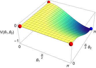
Let us consider a system of two-dimensional rotors, with angular degrees of freedom denoted by with . Taking our cue from the quantum adiabatic search algorithm Roland and Cerf (2002), we allow the rotors to interact via a similar black-box potential. Starting with the potential given in Eq. (I) we demote the Pauli operators to their single-qubit expectation values , ending up with
The above potential attains its minimum value of at (that is, the angle is zero if , and if ) and vanishes for any other angle combination in . The potential is plotted in Fig. 1 for the simple case of with a solution at .
Next, the kinetic energy of the rotors is given by where is a rotor’s moment of inertia (we will choose in the appropriate units). Treating as a source of fluctuations, we consider the following Lagrangian, which interpolates between the kinetic and potential terms:
| (4) |
where is the classical annealing parameter obeying and 111The Lagrangian can be interpreted as a system of rotors with time-varying potential and moments of inertia..
We now ask: how long would it take for the rotors to align into a configuration that minimizes the potential? To answer the question, we set up the initial conditions for the angles and their derivatives such that at , the state of the system minimizes the kinetic energy , namely, and for all (while the latter condition is not strictly necessary for the minimization of the energy, it is chosen so that the angles favor neither zero nor in the beginning 222One could consider a small addition to the kinetic term that would remove the degeneracy of its minima and enforce the condition.).
The Euler-Lagrange equations of motion for the system are
| (5) |
The transformation for all for which simplifies matters, sending the marked state into the all- solution, and along the way transforming all the equations of motion to the set:
| (6) |
Since the transformed angles all evolve in time in an identical manner, the above set of equations may be reduced to a single one by switching to a single variable , yielding:
| (7) |
Equation (7) describes the evolution of a single rotor interpolating between a kinetic term and an effective potential term of the form
| (8) |
This effective potential is plotted in Fig. 2 for various values of . An interesting property of the potential is that it contains no barriers, nor does it have plateaus. It points directly at the correct solution despite becoming more and more shallow with increasing .
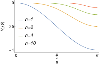
We thus find that the oracular implementation of the potential provides the search space with an important structure.
The equation of motion, Eq. (7), unfortunately has no closed-form solution, making it difficult to find the optimal schedule that would minimize the time to reach from the initial . Nonetheless, a hint as to the performance of the analog algorithm may be gained by studying the special case 333In this case, the algorithm is reminiscent of the analog quantum search algorithm proposed in Ref. Farhi and Gutmann (1996).. In this case, energy is conserved:
| (9) |
and its equation can be integrated to give:
where is the ordinary hypergeometric function. In the large limit, the above expression simplifies to
| (11) |
yielding, asymptotically, a square root scaling with the size of the search space (up to logarithmic corrections).
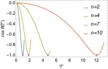
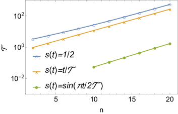
A similar runtime scaling is obtained numerically for two other ‘standard’ schedules, namely, and for . Here, the runtimes are defined as the minimal annealing runtime for which , equivalently, [an example is given in Fig. 3 (top) for a linear schedule]. The minimal runtimes for the above schedules, as a function of size, are depicted in Fig. 3 (bottom), all producing a scaling of (with perhaps additional logarithmic corrections).
It would be instructive to note at this point that the potential governing of the evolution of the rotors does not only have structure, but is also devoid of local minima, a property that in turn leads to a seemingly super-classical performance. Explicitly, the torque it exerts on the rotors always points them towards its minimum. The torque on the -th rotor is given by
Since the term in parenthesis is always negative [it is in fact the potential term for a system of () rotors] the directionality, or sign, of the torque is directly proportional to , the bit that sets its minimizing angle. Determining the minimizing configuration of the potential thus requires only determining the direction in which each of the rotors rotates. Interestingly, the ability to do so hinges on the sensitivity, or resolving power, of the observing device (be it the eye or some type of device). Since the angular resolution of any such device cannot be assumed to scale with system size, the time required to discern the direction in which the rotors move is linearly proportional to the time it takes the rotors to rotate a full quadrant to hit the marked state.
III Effects of finite precision
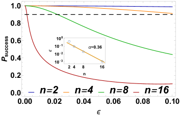
So far, the role that precision requirements play in the performance of the proposed algorithm has not been discussed explicitly. One may ask whether it is indeed the hidden infinite precision that characterizes analog computation that allows for the speedup over digital search. To that aim, we next study the effect of having limited precision on performance by examining the probability of success to find the marked state at the end of the run in the presence small perturbations, or errors, in the initial conditions. Specifically, we consider a deviation in the angles of the rotors at the beginning of the run, namely , where is a small constant. For simplicity, we assume the same error for all angles and consider the schedule . We note though that the effects on performance are expected to be similar, if not more pronounced, for time-varying schedules or in the presence of uncorrelated errors.
The results are summarized in Fig. 4 which depicts the probability of success of the algorithm, , as a function of the initial angle misspecification for different system sizes. As is evident from the figure, the performance of the algorithm is more adversely affected by the perturbation as system size grows. We can quantify this effect by recording the value of for which the probability of success drops by some fixed amount, e.g., as a function of system size. This is shown in the inset of Fig. 4. We find that the allowed error decays exponentially with system size, requiring increasing precision if the quadratic speedup over digital search is to be maintained.
IV Conclusions and discussion
In this study we provided an example of a classical analog construction, inspired by the quantum adiabatic unstructured search algorithm devised by Roland and Cerf Roland and Cerf (2002), for searching an unstructured database. We showed that the required runtime for finding the marked item scales as the square root of the number of elements in the search space, similar to the analogous quantum construction. Since the classical algorithm presented here does not possess any uniquely quantum properties such as entanglement or massive parallelism, the possibility arises that the speedup of the quantum adiabatic search algorithm is a result of it being analog rather than quantum.
We also demonstrated that the classical algorithm is indeed sensitive to small perturbations in the setup, specifically, in initial conditions, as analog algorithms typically are Aaronson (2005); Vergis et al. (1986); Jackson (1960); Albash et al. (2019). We found that the algorithm’s precision requirements increase with problem size if its quadratic speedup is to be maintained. In this context, it is also useful to note again that obtaining the quantum speedup for the Roland and Cerf algorithm requires an ‘exponentially precise’ annealing schedule, as the minimum gap is exponentially localized Childs and Goldstone (2004); Hen (2017); Jonckheere et al. (2013), and that further digitization of the algorithm into a circuit by Trotterization van Dam et al. (2001); Albash and Lidar (2018); Jiang et al. (2017) does not preserve the quadratic quantum speedup Slutskii et al. (2019). Nonetheless, it should be noted that newer algorithms for simulating Hamiltonian evolutions using quantum circuits offer more efficient digitization techniques Berry et al. (2014a, b, 2015); Cleve et al. (2009). These, however, primarily apply to sparse Hamiltonians. It would be interesting to see whether and how much of the quantum advantage of the Roland and Cerf algorithm is sustained if one employs these advanced techniques.
The classical analog construction proposed in this work shares several other key similarities with its quantum adiabatic counterpart. First, in the present algorithm one takes advantage of the symmetries of the problem in order to show that the evolution takes place in a sub-manifold of an exponentially reduced dimensionality, while in the quantum case, one could write down an effective two-by-two Hamiltonian to describe the evolution of the spins in the system. In the classical case the evolution of the two-dimensional rotors is described using an equivalent second-order differential equation. Second, the oracular potential in the present algorithm interpolates between the originally discretized search space states, accepting as input superpositions of digital queries. This property in turn provides the potential for an all-important structure. As we have demonstrated, the added structure to an otherwise unstructured search space is eventually translated to a runtime speedup over the digital unstructured case. One may therefore wonder whether the oracles in both the adiabatic quantum and the analog classical cases are somehow more powerful than intended—especially given their physical infeasibility which may be playing an unintentionally important role.
It should be explicitly noted perhaps that the classical construction proposed here is not meant to be experimentally realizable but was conceived to highlight the potential pitfalls of analog — in this case quantum — algorithms. In light of the results presented here, it would be of interest to therefore rigorously determine whether the quantum adiabatic quadratic speedup for unstructured search is not indeed a consequence of the infinite precision possessed by ideal analog computation (or a too powerful oracle). Of course, similar arguments may also be posed for other quantum analog algorithms. We leave this for future work Slutskii et al. (2019).
Finally, it is also worth noting that the issues raised in this study, namely, the need for infinite precision and the infeasibility of the oracle, do not arise in the context of Grover’s original gate-based algorithm as the latter is not only digital but the unitary operations required to ‘mark’ the sought state can be efficiently carried out Nielsen and Chuang (2000).
Acknowledgements.
We thank Tameem Albash, Elizabeth Crosson, Daniel Lidar and Eleanor Rieffel for insightful discussions. The research is based upon work (partially) supported by the Office of the Director of National Intelligence (ODNI), Intelligence Advanced Research Projects Activity (IARPA), via the U.S. Army Research Office contract W911NF-17-C-0050. The views and conclusions contained herein are those of the authors and should not be interpreted as necessarily representing the official policies or endorsements, either expressed or implied, of the ODNI, IARPA, or the U.S. Government. The U.S. Government is authorized to reproduce and distribute reprints for Governmental purposes notwithstanding any copyright annotation thereon.References
- Shor (1994) P. W. Shor, “Algorithms for quantum computing: discrete logarithms and factoring,” in Proc. 35th Symp. on Foundations of Computer Science, edited by S. Goldwasser (1994) p. 124.
- Grover (1997) L. K. Grover, “Quantum mechanics helps in searching for a needle in a haystack,” Phys. Rev. Lett. 79, 325 (1997).
- Finnila et al. (1994) A.B. Finnila, M.A. Gomez, C. Sebenik, C. Stenson, and J.D. Doll, “Quantum annealing: A new method for minimizing multidimensional functions,” Chemical Physics Letters 219, 343 – 348 (1994).
- Brooke et al. (1999) J. Brooke, D. Bitko, T. F., Rosenbaum, and G. Aeppli, “Quantum annealing of a disordered magnet,” Science 284, 779–781 (1999).
- Kadowaki and Nishimori (1998) T. Kadowaki and H. Nishimori, “Quantum annealing in the transverse Ising model,” Phys. Rev. E 58, 5355 (1998).
- Farhi et al. (2001) E. Farhi, J. Goldstone, S. Gutmann, J. Lapan, A. Lundgren, and D. Preda, “A quantum adiabatic evolution algorithm applied to random instances of an NP-complete problem,” Science 292, 472 (2001).
- Santoro et al. (2002) G. Santoro, R. Martoňák, E. Tosatti, and R. Car, “Theory of quantum annealing of an Ising spin glass,” Science 295, 2427 (2002).
- Vandersypen et al. (2001) L. M. K. Vandersypen, M. Steffen, G. Breyta, C. S. Yannoni, M. H. Sherwood, and I. L. Chuang, “Experimental realization of shor’s quantum factoring algorithm using nuclear magnetic resonance,” Nature 414, 883–887 (2001).
- Bian et al. (2012) Z. Bian, F. Chudak, W. G. Macready, L. Clark, and F. Gaitan, “Experimental determination of ramsey numbers with quantum annealing,” (2012), (arXiv:1201.1842).
- Rønnow et al. (2014) Troels F. Rønnow, Zhihui Wang, Joshua Job, Sergio Boixo, Sergei V. Isakov, David Wecker, John M. Martinis, Daniel A. Lidar, and Matthias Troyer, “Defining and detecting quantum speedup,” Science 345, 420–424 (2014).
- Johnson et al. (2011) M. W. Johnson, M. H. S. Amin, S. Gildert, T. Lanting, F. Hamze, N. Dickson, R. Harris, A. J. Berkley, J. Johansson, P. Bunyk, E. M. Chapple, C. Enderud, J. P. Hilton, K. Karimi, E. Ladizinsky, N. Ladizinsky, T. Oh, I. Perminov, C. Rich, M. C. Thom, E. Tolkacheva, C. J. S. Truncik, S. Uchaikin, J. Wang, B. Wilson, and G. Rose, “Quantum annealing with manufactured spins,” Nature 473, 194–198 (2011).
- Hen et al. (2015) Itay Hen, Joshua Job, Tameem Albash, Troels F. Rønnow, Matthias Troyer, and Daniel A. Lidar, “Probing for quantum speedup in spin-glass problems with planted solutions,” Phys. Rev. A 92, 042325– (2015).
- Boixo et al. (2013) Sergio Boixo, Tameem Albash, Federico M. Spedalieri, Nicholas Chancellor, and Daniel A. Lidar, “Experimental signature of programmable quantum annealing,” Nat. Commun. 4, 2067 (2013).
- Albash et al. (2015) Tameem Albash, Walter Vinci, Anurag Mishra, Paul A. Warburton, and Daniel A. Lidar, “Consistency tests of classical and quantum models for a quantum annealer,” Phys. Rev. A 91, 042314– (2015).
- (15) “Quantum enhanced optimization (qeo),” .
- Tolpygo et al. (2015a) S. K. Tolpygo, V. Bolkhovsky, T. J. Weir, L. M. Johnson, M. A. Gouker, and W. D. Oliver, “Fabrication process and properties of fully-planarized deep-submicron nb/al-alox/nb josephson junctions for vlsi circuits,” IEEE Transactions on Applied Superconductivity 25, 1–12 (2015a).
- Tolpygo et al. (2015b) S. K. Tolpygo, V. Bolkhovsky, T. J. Weir, C. J. Galbraith, L. M. Johnson, M. A. Gouker, and V. K. Semenov, “Inductance of circuit structures for mit ll superconductor electronics fabrication process with 8 niobium layers,” IEEE Transactions on Applied Superconductivity 25, 1–5 (2015b).
- Jin et al. (2015) X. Y. Jin, A. Kamal, A. P. Sears, T. Gudmundsen, D. Hover, J. Miloshi, R. Slattery, F. Yan, J. Yoder, T. P. Orlando, S. Gustavsson, and W. D. Oliver, “Thermal and residual excited-state population in a 3d transmon qubit,” Phys. Rev. Lett. 114, 240501 (2015).
- DW (2) “D-wave systems previews 2000-qubit quantum system,” .
- Young et al. (2008) A. P. Young, S. Knysh, and V. N. Smelyanskiy, “Size dependence of the minimum excitation gap in the Quantum Adiabatic Algorithm,” Phys. Rev. Lett. 101, 170503 (2008), (arXiv:0803.3971) .
- Young et al. (2010) A. P. Young, S. Knysh, and V. N. Smelyanskiy, “First order phase transition in the Quantum Adiabatic Algorithm,” Phys. Rev. Lett. 104, 020502 (2010), (arXiv:0910.1378) .
- Hen and Young (2011) I. Hen and A. P. Young, “Exponential complexity of the quantum adiabatic algorithm for certain satisfiability problems,” Phys. Rev. E. 84, 061152 (2011), arXiv:1109.6872v2 .
- Hen (2012) I. Hen, “Excitation gap from optimized correlation functions in quantum Monte Carlo simulations,” Phys. Rev. E. 85, 036705 (2012), arXiv:1112.2269v2 .
- Farhi et al. (2012) E. Farhi, D. Gosset, I. Hen, A. W. Sandvik, P. Shor, A. P. Young, and F. Zamponi, “Performance of the quantum adiabatic algorithm on random instances of two optimization problems on regular hypergraphs,” Phys. Rev. A 86, 052334 (2012).
- Roland and Cerf (2002) J. Roland and N. J. Cerf, “Quantum search by local adiabatic evolution,” Phys. Rev. A 65, 042308 (2002).
- Farhi and Gutmann (1996) E. Farhi and S. Gutmann, “An Analog Analogue of a Digital Quantum Computation,” eprint arXiv:quant-ph/9612026 (1996), quant-ph/9612026 .
- van Dam et al. (2001) W. van Dam, M. Mosca, and U. Vazirani, “How powerful is adiabatic quantum computation?” in Proceedings 2001 IEEE International Conference on Cluster Computing (2001) pp. 279–287.
- Jansen et al. (2007) S. Jansen, M. B. Ruskai, and R. Seiler, “Bounds for the adiabatic approximation with applications to quantum computation,” J. Math. Phys. 47, 102111 (2007).
- Lidar et al. (2009) D. A. Lidar, A. T. Rezakhani, and A. Hamma, “Adiabatic approximation with exponential accuracy for many-body systems and quantum computation,” J. Math. Phys. 50, 102106 (2009).
- Kato (1951) T. Kato, “On the adiabatic theorem of quantum mechanics,” J. Phys. Soc. Jap. 5, 435 (1951).
- Hen (2014a) I. Hen, “Continuous-time quantum algorithms for unstructured problems,” J. Phys. A: Math. Theor. 47, 045305 (2014a), arXiv:1302.7256 .
- Hen (2014b) Itay Hen, “How fast can quantum annealers count?” Journal of Physics A: Mathematical and Theoretical 47, 235304 (2014b).
- Hen (2017) I. Hen, “Realizable quantum adiabatic search,” EPL (Europhysics Letters) 118, 30003 (2017).
- Roland and Cerf (2003) J. Roland and N. J. Cerf, “Adiabatic quantum search algorithm for structured problems,” Phys. Rev. A 68, 062312 (2003).
- Childs and Goldstone (2004) Andrew M. Childs and Jeffrey Goldstone, “Spatial search by quantum walk,” Phys. Rev. A 70, 022314 (2004).
- Albash and Lidar (2018) Tameem Albash and Daniel A. Lidar, “Adiabatic quantum computation,” Rev. Mod. Phys. 90, 015002 (2018).
- Jiang et al. (2017) Zhang Jiang, Eleanor G. Rieffel, and Zhihui Wang, “Near-optimal quantum circuit for grover’s unstructured search using a transverse field,” Phys. Rev. A 95, 062317 (2017).
- Aaronson (2005) Scott Aaronson, “Guest column: Np-complete problems and physical reality,” SIGACT News 36, 30–52 (2005).
- Vergis et al. (1986) Anastasios Vergis, Kenneth Steiglitz, and Bradley Dickinson, “The complexity of analog computation,” Mathematics and Computers in Simulation 28, 91 – 113 (1986).
- Jackson (1960) Albert S. Jackson, Analog Computation (McGraw-Hill, New York, USA, 1960).
- Albash et al. (2019) T. Albash, V. Martin-Mayor, and I. Hen, “Analog Errors in Ising Machines,” accepted for publication in Quantum Science & Technology (2019), arXiv:1806.03744 [quant-ph] .
- Note (1) The Lagrangian can be interpreted as a system of rotors with time-varying potential and moments of inertia.
- Note (2) One could consider a small addition to the kinetic term that would remove the degeneracy of its minima and enforce the condition.
- Note (3) In this case, the algorithm is reminiscent of the analog quantum search algorithm proposed in Ref. Farhi and Gutmann (1996).
- Jonckheere et al. (2013) Edmond A. Jonckheere, Ali T. Rezakhani, and Farooq Ahmad, “Differential topology of adiabatically controlled quantum processes,” Quantum Information Processing 12, 1515–1538 (2013).
- Slutskii et al. (2019) Mikhail Slutskii, Tameem Albash, Lev Barash, and Itay Hen, “Analog Nature of Quantum Adiabatic Unstructured Search,” arXiv e-prints , arXiv:1904.04420 (2019), arXiv:1904.04420 [quant-ph] .
- Berry et al. (2014a) Dominic W. Berry, Richard Cleve, and Sevag Gharibian, “Gate-efficient discrete simulations of continuous-time quantum query algorithms,” Quantum Info. Comput. 14, 1–30 (2014a).
- Berry et al. (2014b) Dominic W. Berry, Andrew M. Childs, Richard Cleve, Robin Kothari, and Rolando D. Somma, “Exponential improvement in precision for simulating sparse hamiltonians,” in Proceedings of the Forty-sixth Annual ACM Symposium on Theory of Computing, STOC ’14 (ACM, New York, NY, USA, 2014) pp. 283–292.
- Berry et al. (2015) Dominic W. Berry, Andrew M. Childs, Richard Cleve, Robin Kothari, and Rolando D. Somma, “Simulating hamiltonian dynamics with a truncated taylor series,” Phys. Rev. Lett. 114, 090502 (2015).
- Cleve et al. (2009) Richard Cleve, Daniel Gottesman, Michele Mosca, Rolando D. Somma, and David Yonge-Mallo, “Efficient discrete-time simulations of continuous-time quantum query algorithms,” in Proceedings of the Forty-first Annual ACM Symposium on Theory of Computing, STOC ’09 (ACM, New York, NY, USA, 2009) pp. 409–416.
- Nielsen and Chuang (2000) M. A. Nielsen and I. L. Chuang, Quantum Computation and Quantum Information (Cambridge University Press, Cambridge, England, 2000).