A novel derivation of the Marchenko-Pastur law through analog bipartite spin-glasses

Abstract

In the last decades, statistical mechanics of disordered systems (mainly spin glasses) has become one of the main tool to investigate complex systems, probably due to the celebrated Replica Symmetry Breaking scheme of Parisi Theory and its deep implications.
In this work we consider the analog bipartite spin-glass (or real-valued restricted Boltzmann machine in a neural network jargon), whose variables (those quenched as well as those dynamical) share standard Gaussian distributions. First, via Guerra’s interpolation technique, we express its quenched free energy in terms of the natural order parameters of the theory (namely the self- and two-replica overlaps), then, we re-obtain the same result by using the replica-trick: a mandatory tribute, given the special occasion. Next, we show that the quenched free energy of this model is the functional generator of the moments of the correlation matrix among the weights connecting the two layers of the spin-glass (i.e., the Wishart matrix in random matrix theory or the Hebbian coupling in neural networks): as weights are quenched stochastic variables, this plays as a novel tool to inspect random matrices. In particular, we find that the Stieltjes transform of the spectral density of the correlation matrix is determined by the (replica-symmetric) quenched free energy of the bipartite spin-glass model. In this setup, we re-obtain the Marchenko-Pastur law in a very simple way.

1 Introduction

It did not take long for scientists to realize the impressive representational power of the Sherrington-Kirkpatrick model (i.e., the simplest mean-field spin glass), especially in relation to its low temperature behaviour with the spontaneous hierarchical organization of its thermodynamical states, as painted by Parisi at the turn of the seventies and eighties Giorgio1 ; Giorgio2 ; Giorgio3 (and duly mathematically confirmed in recent times by Guerra Guerra-Broken , Panchencko Panchenko and Talagrand talaProof ). Since then, spin glasses quickly became the harmonic oscillators of complex systems, with applications ranging from Biology to Engineering. As for the former, the spin-glass framework applies over different scales, from the extracellular world of neural Albert2 ; Giorgio-Neural and immune Agliari-Immune ; Giorgio-Immune networks to the inner world of protein folding protein and gene regulatory networks gene and even questioning about evolution Kaufmann ; Peliti ; as for the latter, spin-glasses are extensively exploited in machine learning Coolen ; Giorgio-Learning and computer science Zecchina1 ; Zecchina2 , tackling computational complexity from an entirely statistical-mechanics driven perspective CompCompl ; Nishimori (of course, this is far from being an exhaustive list). Further, spin-glass theory gave several hints even in more theoretical contexts (quoting Talagrand, “spin glasses are heaven for mathematicians” Tala ) as their studies inspired several fields of Mathematics such as random matrix theory RMT , variational calculus Auffinger , probability theory Bovierbook , PDE theory dynamic and much more.
In this paper we investigate a hidden link between bipartite spin-glasses and the Marchenko-Pastur law. To this goal we consider a fully analog bipartite system, whose quenched and dynamical variables (i.e., the couplings and the spins, respectively) are all drawn from a normal distribution $\mathcal{N}[0,1]$, and we look for an explicit expression of its quenched free energy: this is achieved by means of Guerra’s interpolating technique and, independently, by means of the celebrated replica trick. Once the resulting free energy is extremized over the order parameters, en route for their self-consistent expression, we obtain the latter in terms of an algebraic set of equations, whose solution captures the momenta of the Wishart matrix stemming from the weights among the two parties.
More explicitely, if the two parties have sizes $N$ and $P=\alpha N$ (with $\alpha\in\mathbb{R}^{+}$), we can define their mutual connections via a weight matrix $\xi_{i}^{\mu}$ ($i\in(1,...,N)$ and $\mu\in(1,...,P)$), such that the weight correlation matrix reads as $C_{\mu\nu}=N^{-1}\sum_{i}^{N}\xi_{i}^{\mu}\xi_{j}^{\mu}$. Notice that, by definition, the matrix $\mathbb{C}$ is, according to the perspective, a Wishart matrix as well as a Hebbian kernel Amit ; Coolen and its spectrum obeys the well-known Marchenko-Pastur law. Then, we prove that the quenched free energy of the fully analog bipartite spin glass is the generating functional of the moments of such a correlation matrix. This link allows the usage of the Stieltjes-Perron inversion formula to reconstruct the spectral density of the correlation matrix, thus obtaining, from a pure statistical mechanics framework, the Marchenko-Pastur distribution.
Extensive comparison between our theory and simulations shows full agreement between the analytical and the numerical sides of the present investigation.
As a final remark we stress that another powerful link between Disordered Statistical Mechanics and Random Matrix Theory was settled in Kuhn where the Wigner semicircle distribution and the Marchenko-Pastur law were re-obtained by an extensive use of the cavity field technique, another primary technique in spin-glasses Barra-JSP2006 ; GuerraCavity ; MP0 ; MPV , but directly applied in a pure random matrix context.

2 The analog bi-partite spin-glass

We start by introducing the model, described by the following energy cost function

$$E(\boldsymbol{z},\boldsymbol{\varphi}|\xi):=-\frac{1}{\sqrt{N}}\sum_{\mu,i}^{P,N}\xi^{\mu}_{i}z_{\mu}\varphi_{i}.$$ (1)

This is a bipartite system composed by two different layers of standard Gaussian variables $z_{\mu}$ and $\varphi_{i}$ with symmetric interactions $\xi_{i}^{\mu}$, whose strength is also sampled i.i.d. from $\mathcal{N}[0,1]$. The indices $i$ and $\mu$ run respectively in the ranges $1,\dots,N$ and $1,\dots,P$. We will consider the so-called high-storage case where $P=\alpha N$, with $\alpha\in\mathbb{R}^{+}$, for large $N$, namely the challenging regime to explore when studying bipartite spin glasses bipartiti ; how-glassy or restricted Boltzmann machines Agliari-Dantoni ; Coolen (and the related Hopfield model Agliari-PRL1 ; Albert1 ; Albert2 ; Mezard ; Monasson ).
The partition function for such a system is therefore defined as

$$Z_{N,P}(\beta|\xi):=\int d\mu(\boldsymbol{z},\boldsymbol{\varphi})\exp\Big{(}\frac{\beta}{\sqrt{N}}\sum_{\mu,i}^{P,N}\xi^{\mu}_{i}z_{\mu}\varphi_{i}\Big{)},$$ (2)

where $\beta\in\mathbb{R}^{+}$ tunes the level of noise and

$$d\mu(\boldsymbol{z},\boldsymbol{\varphi}):=\prod_{\mu,i}^{P,N}\frac{dz_{\mu}}{\sqrt{2\pi}}\exp(-z_{\mu}^{2}/2)\frac{d\varphi_{i}}{\sqrt{2\pi}}\exp(-\varphi_{i}^{2}/2)$$ (3)

is the multidimensional Gaussian measure. The key quantity to study in order to have a picture of the properties of the model is its quenched free-energy defined as

$$\mathit{f}(\alpha,\beta):=\lim_{N\to\infty}\frac{1}{N}\mathbb{E}_{\xi}\log\int d\mu(\boldsymbol{z},\boldsymbol{\varphi})\exp\Big{(}\frac{\beta}{\sqrt{N}}\sum_{\mu,i}^{P,N}\xi^{\mu}_{i}z_{\mu}\varphi_{i}\Big{)},$$ (4)

where $\mathbb{E}_{\xi}$ is the average over all possible weight (or coupling or pattern) realizations, i.e.

$$\mathbb{E}_{x}f(x)=\int dxf(x)e^{-x^{2}/2}.$$

3 Replica symmetric solution of the quenched free energy

3.1 The interpolation scheme

The computation of the quenched free energy in the thermodynamic limit can be performed by means of a Guerra’s interpolation method (whose genesis lies in the treatment of the analog Hopfield model Barra-JSP2010 ). More precisely, once introduced an interpolating parameter $s\in(0,1)$, the scalars $A,B,C,D$ (whose explicit values will be set a fortiori), $N$ i.i.d. Gaussian fields $\eta_{i}\sim\mathcal{N}[0,1]$, $i\in(1,...,N)$ and $P$ i.i.d. Gaussian fields $\psi_{\mu}\sim\mathcal{N}[0,1]$, $\mu\in(1,...,P)$, the interpolating free energy is defined as

$$\begin{split}\mathit{f}(s):=\frac{1}{N}\mathbb{E}_{\xi,\eta,\psi}\log\int d\mu(\boldsymbol{z},\boldsymbol{\varphi})\exp&\Big{[}\sqrt{s}\frac{\beta}{\sqrt{N}}\sum_{\mu i}\xi^{\mu}_{i}z_{\mu}\varphi_{i}\\ &+\sqrt{1-s}(A\sum_{i}\eta_{i}\varphi_{i}+B\sum_{\mu}\psi_{\mu}z_{\mu})\\ &+\frac{1-s}{2}(C\sum_{\mu}z_{\mu}^{2}+D\sum_{i}\varphi_{i}^{2})\Big{]}.\end{split}$$ (5)

In the first line, we introduced the contribution coming from the model under consideration (which is of course reproduced for $s=1$, i.e., in the thermodynamic limit $f(s=1)=f(\alpha,\beta)$); the second line is an effective mean-field contribution, statistically representing the external field produced by each layer on the other one (but where we replaced the original two-body interactions with a one-body coupling); the third line contains terms necessary to properly rescale the second moments of the dynamical variables $(\boldsymbol{z},\boldsymbol{\varphi})$.
Note that now the average $\mathbb{E}_{\xi}$ over quenched variables has to be replaced by $\mathbb{E}_{\xi,\eta,\psi}\equiv\mathbb{E}$ such that the average is performed over all the quenched random variables, as stressed by the subscript.
In order to compute the free energy of the system (2), we adopt the elementary sum rule

$$\mathit{f}(s=1)=\mathit{f}(s=0)+\int_{0}^{1}\frac{df(s)}{ds}ds.$$ (6)

The computation of the derivative in (6) is straightforward:

$$\begin{split}\frac{df(s)}{ds}=\frac{1}{N}\mathbb{E}\Bigg{[}&\frac{1}{2\sqrt{s}}\frac{\beta}{\sqrt{N}}\sum_{i,\mu=1}^{N,P}\xi^{\mu}_{i}\langle z_{\mu}\varphi_{i}\rangle-\frac{1}{2\sqrt{1-s}}\left(A\sum_{i=1}^{N}\eta_{i}\langle\varphi_{i}\rangle+B\sum_{\mu=1}^{P}\psi_{\mu}\langle z_{\mu}\rangle\right)\\ &-\frac{1}{2}\left(C\sum_{\mu=1}^{P}\langle z_{\mu}^{2}\rangle+D\sum_{i=1}^{N}\langle\varphi_{i}^{2}\rangle\right)\Bigg{]}.\end{split}$$ (7)

By simple applications of the Wick theorem [$\mathbb{E}_{x}xF(x)=\mathbb{E}_{x}\partial_{x}F(x)$] over the Gaussian variables, we have

$$\begin{split}\mathbb{E}\,\xi^{\mu}_{i}\langle z_{\mu}\varphi_{i}\rangle&=\sqrt{s/N}\beta\leavevmode\nobreak\ \mathbb{E}\,(\langle z_{\mu}^{2}\varphi_{i}^{2}\rangle-\langle z_{\mu}\varphi_{i}\rangle^{2}),\\ \mathbb{E}\,\eta_{i}\langle\varphi_{i}\rangle&=A\sqrt{1-s}\leavevmode\nobreak\ \mathbb{E}\,(\langle\varphi_{i}^{2}\rangle-\langle\varphi_{i}\rangle^{2}),\\ \mathbb{E}\,\psi_{\mu}\langle z_{\mu}\rangle&=B\sqrt{1-s}\leavevmode\nobreak\ \mathbb{E}\,(\langle z_{\mu}^{2}\rangle-\langle z_{\mu}\rangle^{2}).\end{split}$$ (8)

Then,

$$\begin{split}\frac{df(s)}{ds}=&\frac{1}{N}\mathbb{E}\Big{[}\frac{\beta^{2}}{2N}\sum_{\mu,i=1}^{P,N}(\langle z_{\mu}^{2}\varphi_{i}^{2}\rangle-\langle z_{\mu}\varphi_{i}\rangle^{2})-\frac{A^{2}}{2}\sum_{i=1}^{N}(\langle\varphi_{i}^{2}\rangle-\langle\varphi_{i}\rangle^{2})-\frac{B^{2}}{2}\sum_{\mu=1}^{P}(\langle z_{\mu}^{2}\rangle-\langle z_{\mu}\rangle^{2})\\ &-\frac{1}{2}(C\sum_{\mu=1}^{P}\langle z_{\mu}^{2}\rangle+D\sum_{i=1}^{N}\langle\varphi_{i}^{2}\rangle)\Big{]}\end{split}$$ (9)

We now introduce the self- and the two-replica overlaps within each layer, respectively as

$$\begin{split}q_{11}&=\frac{1}{N}\sum_{i=1}^{N}\varphi_{i}^{2},\qquad\qquad p_{11}=\frac{1}{P}\sum_{\mu=1}^{P}z_{\mu}^{2},\\ q_{12}&=\frac{1}{N}\sum_{i=1}^{N}\varphi_{i}^{(1)}\varphi_{i}^{(2)},\qquad p_{12}=\frac{1}{P}\sum_{\mu=1}^{P}z_{\mu}^{(1)}z_{\mu}^{(2)},\end{split}$$ (10)

where the superscript $(1),(2)$ are replica indices, and we use these overlaps to recast the r.h.s. of eq. (9) as

$$\begin{split}\frac{df(s)}{ds}=\frac{\alpha\beta^{2}}{2}\mathbb{E}\Big{[}&\langle p_{11}q_{11}\rangle-\frac{A^{2}+D}{\alpha\beta^{2}}\langle q_{11}\rangle-\frac{B^{2}+C}{\beta^{2}}\langle p_{11}\rangle-(\langle p_{12}q_{12}\rangle-\frac{A^{2}}{\alpha\beta^{2}}\langle q_{12}\rangle-\frac{B^{2}}{\beta^{2}}\langle p_{12}\rangle)\Big{]}.\end{split}$$ (11)

Finally, by choosing

$$A=\beta\sqrt{q_{N}},\quad B=\beta\sqrt{p_{N}},\quad C=\beta^{2}(q_{D}-q_{N}),\quad D=\alpha\beta^{2}(p_{D}-p_{N}),$$ (12)

we can rewrite the streaming of the interpolating free energy as

$$\frac{df(s)}{ds}=\frac{\alpha\beta^{2}}{2}\mathbb{E}\Big{[}\langle(p_{11}-p_{D})(q_{11}-q_{D})\rangle-p_{D}q_{D}-(\langle(p_{12}-p_{N})(q_{12}-q_{N})\rangle-p_{N}q_{N})\Big{]}.$$ (13)

The crucial point now is to fix $q_{D,N}$ and $p_{D,N}$. We notice that, in a replica-symmetry regime, the overlaps converge to their average values (meaning that fluctuations are suppressed) in the thermodynamic limit. Therefore, if we interpret $q_{D,N}$ and $p_{D,N}$ as respectively the (self-averaging) equilibrium values of the diagonal and non-diagonal overlaps in the thermodynamic limit, we simply have $d_{s}f(s)=\tfrac{\alpha\beta^{2}}{2}p_{N}q_{N}-\tfrac{\alpha\beta^{2}}{2}p_{D}q_{D}$, that is clearly $s$-independent. Consequently, the integral in the sum rule (6) is trivial as it coincides with the multiplication by one.

The one-body term (i.e., $f(s=0)$) is easy to evaluate, since it is a one-body calculation, returning

$$\begin{split}f(s=0)&=\frac{1}{N}\mathbb{E}\ln\int d\mu(\boldsymbol{z},\boldsymbol{\varphi})\exp\Big{(}A\sum_{i}\eta_{i}\varphi_{i}+B\sum_{\mu}\psi_{\mu}z_{\mu}+C\sum_{\mu}z_{\mu}^{2}+D\sum_{i}\varphi_{i}^{2}\Big{)}=\\ &=-\frac{\alpha}{2}\log(1-C)-\frac{1}{2}\log(1-D)+\frac{A^{2}}{2(1-D)}+\frac{\alpha B^{2}}{2(1-C)}.\end{split}$$ (14)

By combining (6), (13) and (14), we get the quenched free energy related to the analog bipartite spin-glass as

$$\begin{split}f(\alpha,\beta)=&-\frac{\alpha}{2}\log[1-\beta^{2}(q_{D}-q_{N})]-\frac{1}{2}\log[1-\alpha\beta^{2}(p_{D}-p_{N})]\\ &+\frac{\alpha\beta^{2}p_{N}}{2[1-\alpha\beta^{2}(p_{D}-p_{N})]}+\frac{\alpha\beta^{2}q_{N}}{2[1-\beta^{2}(q_{D}-q_{N})]}+\frac{\alpha\beta^{2}}{2}p_{N}q_{N}-\frac{\alpha\beta^{2}}{2}p_{D}q_{D}.\end{split}$$ (15)

3.2 The replica trick route

To conclude this investigation, recalling that this is a dedicated contribution to celebrate the seventieth birthday of Giorgio Parisi, it seems mandatory to re-obtain the previous results with the first route paved in order to embed replica symmetry breaking into a mathematical framework: the replica trick MPV . In the original replica-trick framework MPV , the quenched free energy is represented as

$$f(\alpha,\beta)=\lim_{N\rightarrow\infty}\lim_{n\rightarrow 0}\frac{\mathbb{E}Z_{N,P}^{n}(\beta|\xi)-1}{nN}.$$ (16)

The $n$-th power of the partition function is therefore naturally expressed in terms of replicas as

$$Z_{N,P}^{n}(\beta|\xi)=\prod_{\gamma=1}^{n}Z_{N,P}^{(\gamma)}(\beta|\xi)=\int\left(\prod_{\gamma=1}^{n}d\mu(\boldsymbol{z}^{\gamma},\boldsymbol{\varphi}^{\gamma})\right)\exp\Big{(}\frac{\beta}{\sqrt{N}}\sum_{i,\mu,\gamma=1}^{N,P,n}\xi^{\mu}_{i}z_{\mu}^{\gamma}\varphi^{\gamma}_{i}\Big{)}.$$ (17)

In this way, one can directly perform the average over the quenched noise (the couplings $\boldsymbol{\xi}$), so that

$$\mathbb{E}Z_{N,P}^{n}(\beta|\xi)=\int\left(\prod_{\gamma}d\mu(\boldsymbol{z}^{\gamma},\boldsymbol{\varphi}^{\gamma})\right)\exp\Big{(}\frac{\beta^{2}}{2N}\sum_{i,\mu}\sum_{\gamma,\delta}z_{\mu}^{\gamma}z_{\mu}^{\delta}\varphi^{\gamma}_{i}\varphi^{\delta}_{i}\Big{)}.$$ (18)

In order to linearize the problem in the dynamical variables, one can introduce the overlaps in each layer by inserting, for each kind of overlap and for each couple of replicas, a Dirac delta, namely

$$\delta(q_{\gamma\delta}-N^{-1}\sum_{i}\varphi_{i}^{\gamma}\varphi_{i}^{\delta})\delta(p_{\gamma\delta}-P^{-1}\sum_{\mu}z_{\mu}^{\gamma}z_{\mu}^{\delta}),$$ (19)

then, by using the Fourier representation of the delta function, we can rewrite the partition function as

$$\begin{split}\mathbb{E}Z_{N,P}^{n}(\beta|\xi)&=\int\left(\prod_{\gamma}d\mu(\boldsymbol{z}^{\gamma},\boldsymbol{\varphi}^{\gamma})\right)\left(\prod_{\gamma,\delta}dq_{\gamma\delta}dp_{\gamma\delta}\frac{Nd\bar{q}_{\gamma\delta}}{2\pi}\frac{Pd\bar{q}_{\gamma\delta}}{2\pi}\right)\times\\ &\times\exp\Big{(}iN\sum_{\gamma,\delta}\bar{q}_{\gamma\delta}(q_{\gamma\delta}-\tfrac{1}{N}\sum_{i}\varphi_{i}^{\gamma}\varphi_{i}^{\delta})+iP\sum_{\gamma,\delta}\bar{p}_{\gamma\delta}(p_{\gamma\delta}-\tfrac{1}{P}\sum_{\mu}z_{\mu}^{\gamma}z_{\mu}^{\delta})+\frac{\beta^{2}P}{2}\sum_{\gamma,\delta}p_{\gamma\delta}q_{\gamma\delta}\Big{)},\end{split}$$ (20)

where $\bar{q}_{\gamma\delta}$ and $\bar{p}_{\gamma\delta}$ are, respectively, the conjugates of $q_{\gamma\delta}$ and $p_{\gamma\delta}$, for any $\gamma,\delta=1,...,n$. At this point, we can easily perform the Gaussian integration over the dynamical variables, yielding (after a trivial rescaling of the conjugates $\bar{q}_{\gamma\delta}\rightarrow 2^{-1}i\bar{q}_{\gamma\delta}$ and $\bar{p}_{\gamma\delta}\rightarrow 2^{-1}i\bar{p}_{\gamma\delta}$)

$$\begin{split}\mathbb{E}Z^{n}_{N,P}(\beta|\xi)&=\int\left(\prod_{\gamma\delta}dq_{\gamma\delta}dp_{\gamma\delta}\frac{iNd\bar{q}_{\gamma\delta}}{4\pi}\frac{iPd\bar{q}_{\gamma\delta}}{4\pi}\right)\times\\ &\times\exp\Big{(}-\frac{N}{2}\sum_{\gamma\delta}\bar{q}_{\gamma\delta}q_{\gamma\delta}-\frac{\alpha N}{2}\sum_{\gamma\delta}\bar{p}_{\gamma\delta}p_{\gamma\delta}+\frac{\alpha\beta^{2}N}{2}\sum_{\gamma\delta}p_{\gamma\delta}q_{\gamma\delta}\\ &-\frac{\alpha N}{2}\log\det(1-\bar{\boldsymbol{p}})-\frac{N}{2}\log\det(1-\bar{\boldsymbol{q}})\Big{)},\end{split}$$ (21)

where $\bar{\boldsymbol{q}}$ and $\bar{\boldsymbol{p}}$ are the conjugate overlap matrices. By taking the intensive logarithm of the expression above, we get the following quenched free energy

$$\begin{split}f(\alpha,\beta)&=-\frac{1}{2n}\sum_{\gamma\delta}\bar{q}_{\gamma\delta}q_{\gamma\delta}-\frac{\alpha}{2n}\sum_{\gamma\delta}\bar{p}_{\gamma\delta}p_{\gamma\delta}+\frac{\alpha\beta^{2}}{2n}\sum_{\gamma\delta}p_{\gamma\delta}q_{\gamma\delta}\\ &-\frac{\alpha}{2n}\log\det(1-\bar{\boldsymbol{p}})-\frac{1}{2n}\log\det(1-\bar{\boldsymbol{q}}).\end{split}$$ (22)

The replica symmetry ansatz, in this context, reads as

$$\begin{split}q_{\gamma\delta}=&q_{D}\delta_{\gamma\delta}+q_{N}(1-\delta_{\gamma\delta}),\\ p_{\gamma\delta}=&p_{D}\delta_{\gamma\delta}+p_{N}(1-\delta_{\gamma\delta}),\\ \bar{q}_{\gamma\delta}=&\bar{q}_{D}\delta_{\gamma\delta}+\bar{q}_{N}(1-\delta_{\gamma\delta}),\\ \bar{p}_{\gamma\delta}=&\bar{p}_{D}\delta_{\gamma\delta}+\bar{p}_{N}(1-\delta_{\gamma\delta}).\end{split}$$ (23)

Then, by straightforward computations, assuming the commutativity of the infinite volume limit and the zero-replica limit, we have

$$\begin{split}f(\alpha,\beta)&=\frac{\alpha\beta^{2}}{2}(p_{D}q_{D}-p_{N}q_{N})-\frac{\alpha}{2}(\bar{p}_{D}p_{D}-\bar{p}_{N}p_{N})-\frac{1}{2}(\bar{q}_{D}q_{D}-\bar{q}_{N}q_{N})\\ &-\frac{\alpha}{2}\Big{(}\log[1-\bar{p}_{D}+\bar{p}_{N}]-\frac{\bar{p}_{N}}{1-\bar{p}_{D}+\bar{p}_{N}}\Big{)}-\frac{1}{2}\Big{(}\log[1-\bar{q}_{D}+\bar{q}_{N}]-\frac{\bar{q}_{N}}{1-\bar{q}_{D}+\bar{q}_{N}}\Big{)}.\end{split}$$ (24)

On the saddle point, we find the following self-consistency equations for the conjugates order parameters:

$$\bar{q}_{D}=\alpha\beta^{2}p_{D},\quad\bar{p}_{D}=\beta^{2}q_{D},\quad\bar{q}_{N}=\alpha\beta^{2}p_{N},\quad\bar{p}_{N}=\beta^{2}q_{N}.$$ (25)

By inserting these equations in the formula (24), one precisely finds the expression (15) for the quenched free energy.

3.3 Self-consistency equations and extremal free energy

In order to find the explicit expression for the quenched free energy as a function of the system parameters $(\alpha,\beta)$ the expression (15) must be extremized with respect to the order parameters $q_{D,N}$, $p_{D,N}$. To this goal it is convenient to rewrite the quenched free energy in terms of the two new order parameters

$$\begin{split}\Delta_{q}&=q_{D}-q_{N},\\ \Delta_{p}&=p_{D}-p_{N},\end{split}$$ (26)

i.e., the difference between the diagonal and non-diagonal overlaps. In this way, the quenched free energy can be rewritten as

$$\begin{split}f(\alpha,\beta)=&-\frac{\alpha}{2}\log(1-\beta^{2}\Delta_{q})-\frac{1}{2}\log(1-\alpha\beta^{2}\Delta_{p})\\ &+\frac{\alpha\beta^{2}p_{N}}{2(1-\alpha\beta^{2}\Delta_{p})}+\frac{\alpha\beta^{2}q_{N}}{2(1-\beta^{2}\Delta_{q})}-\frac{\alpha\beta^{2}}{2}(p_{N}\Delta_{q}+q_{N}\Delta_{p}+\Delta_{q}\Delta_{p}).\end{split}$$ (27)

By imposing the extremality condition on the quenched free energy, for these order parameters we find algebraic self-consistency equations, namely

$$\Delta_{p}=\frac{1}{1-\beta^{2}\Delta_{q}},\quad\Delta_{q}=\frac{1}{1-\alpha\beta^{2}\Delta_{p}},\quad q_{N}=\alpha\beta^{2}p_{N}\Delta_{q}^{2},\quad p_{N}=\beta^{2}q_{N}\Delta_{p}^{2}.$$ (28)

By solving this algebraic system, beyond the trivial solution $p_{N}=q_{N}=0$ for non-diagonal overlaps, we get

$$\begin{split}q_{D}\equiv\Delta_{q}&=\frac{1+(1-\alpha)\beta^{2}-\sqrt{(1+\beta^{2}-\alpha\beta^{2})^{2}-4\beta^{2}}}{2\alpha\beta^{2}},\\ p_{D}\equiv\Delta_{p}&=\frac{1-(1-\alpha)\beta^{2}-\sqrt{(1+\beta^{2}-\alpha\beta^{2})^{2}-4\beta^{2}}}{2\alpha\beta^{2}}.\end{split}$$ (29)

By plugging these expressions in the quenched free energy (27), the final result reads as

$$\begin{split}f(\alpha,\beta)&=\frac{\alpha\beta^{2}+\beta^{2}-1+\sqrt{(\alpha-1)^{2}\beta^{4}-2(\alpha+1)\beta^{2}+1}}{4\beta^{2}}\\ &-\frac{\alpha}{2}\log\Big{(}\frac{1}{2}[(\alpha-1)\beta^{2}+\sqrt{(\alpha-1)^{2}\beta^{4}-2(\alpha+1)\beta^{2}+1}+1]\Big{)}\\ &-\frac{1}{2}\log\Big{(}\frac{1}{2}[(1-\alpha)\beta^{2}+\sqrt{(\alpha-1)^{2}\beta^{4}-2(\alpha+1)\beta^{2}+1}+1]\Big{)},\end{split}$$ (30)

namely, the r.h.s. of eq. (30) is the explicit expression of the extremal quenched free energy in the replica symmetric regime for the bipartite Gaussian spin-glass (1).

4 Bi-partite spin glasses and the Marchenko-Pastur law

Random matrix theory Mehta ; Tao ; Vulpiani raised around the early decades of the past century in the context of multivariate statistics by pioneers as Wishart Wishart and Hsu Hsu and probably became a discipline by its own since, in the fifties, Wigner systematically developed its foundations Wigner . The crucial point is that, for several problems, in the asymptotic regime (i.e., in the thermodynamic limit), random matrices exhibit universality, namely results become independent of the details of the original probability distributions generating the entries. Remarkably, universality is also a well identified property of spin glasses Univ1 ; Univ2 .
For instance, the eigenvalue distribution of a real symmetric matrix, whose random entries are independently distributed with equal densities, converges to Wigner’s semicircle law regardless of the details of the underlying entry densities.
Another fundamental distribution is the one named after Marchenko and Pastur, who gave the limiting distribution of eigenvalues of Wishart matrices. More precisely, the main results concerning the Marchenko-Pastur distribution can be summarized as follows. Let $P$ be a sequence of integers such that $P=\alpha N$ with $\alpha\in\mathbb{R}^{+}$ and consider an $N\times P$ matrix $\boldsymbol{\xi}$ whose entries are i.i.d. standard Gaussian variables, i.e., $\xi_{i}^{\mu}\sim\mathcal{N}[0,1]$ for any $i=1,..,N$ and $\mu=1,...,P$. Normalize this matrix to get $\boldsymbol{\hat{\xi}}:=\boldsymbol{\xi}/\sqrt{N}$ and construct $\mathbf{C}=\boldsymbol{\hat{\xi}}\boldsymbol{\hat{\xi}}^{T}$ that is symmetric (hence has real eingenvalues $\gamma_{1},...,\gamma_{N}$) with spectral distribution referred to as $\rho(\gamma)$. Then, the Marchenko-Pastur theorem guarantees that $\rho(\gamma)$ (weakly) converges to the distribution, defined for $\gamma\in[\gamma_{-},\gamma_{+}]$

$$\rho(\gamma) = \frac{\sqrt{(\gamma-\gamma_{-})(\gamma-\gamma_{+})}}{2\pi\gamma}\mathbb{1}_{\gamma\in[\gamma_{-},\gamma_{+}]},$$ (31)

$$\gamma_{-} = (1-\sqrt{\alpha})^{2},\ \ \ \gamma_{+}=(1+\sqrt{\alpha})^{2},$$ (32)

that is called the Marchenko-Pastur distribution.

4.1 Another link between Random Matrices and Statistical Mechanics

An interesting application of the solution of the analog bipartite spin-glass lies exactly in random matrix theory, as we are going to show in this subsection. The partition function under consideration (see eq. (2)) is of trivial solution via standard Gaussian integration. In fact, by direct calculations, one gets

$$Z_{N,P}(\beta|\xi)={\det}^{-1/2}(1-\beta^{2}\mathbf{C}),$$ (33)

where we defined the correlation matrix of the couplings as

$$C_{\mu\nu}=\frac{1}{N}\sum_{i=1}^{N}\xi^{\mu}_{i}\xi^{\nu}_{i}.$$ (34)

It is worth stressing that $\mathbf{C}$ is known as Wishart matrix in the random matrix theory and, also, it is exactly the Hebbian kernel adopted in neural networks Amit .
When $\beta^{2}\lVert\mathbf{C}\rVert<1$, we expand the determinant as

$$\det(1-\beta^{2}\mathbf{C})=\exp\left(-\sum_{k=1}^{\infty}\frac{\text{Tr }\beta^{2}\mathbf{\mathbf{C}}^{n}}{n}\right).$$ (35)

Taking the logarithm of the partition function (as coded at the r.h.s. of eq. (33)) results in the following relation

$$\log Z_{N,P}(\beta|\xi)=\frac{1}{2}\sum_{k=1}^{\infty}\frac{\beta^{2k}\text{Tr }\mathbf{C}^{k}}{k}.$$ (36)

Finally, taking the average over the weight realizations and taking the $N\rightarrow\infty$ limit after multiplying by $1/N$, we have

$$f(\alpha,\beta)=\frac{1}{2}\sum_{k=1}^{\infty}\frac{\beta^{2k}}{k}c_{k},$$ (37)

where

$$c_{k}=\lim_{N\rightarrow\infty}\frac{1}{N}\mathbb{E}_{\xi}\text{Tr }\mathbf{C}^{k}.$$ (38)

In other words, the quenched free energy of the model (1) is the generating function of the moments of the correlation matrix of the weights (i.e. of the patterns in a neural network jargon). Therefore, we can now generate them with the elementary formula

$$\lim_{N\rightarrow\infty}\frac{1}{N}\mathbb{E}_{\xi}\text{Tr }\mathbf{C}^{n}=\frac{2n}{n!}\Big{(}\frac{d}{d\beta^{2}}\Big{)}^{n}f\Big{|}_{\beta=0}.$$ (39)

From random matrix theory, we know that the momenta of Wishart matrix capture all the information about its spectrum. Indeed,

$$\lim_{N\rightarrow\infty}\frac{1}{N}\mathbb{E}_{\xi}\,\text{Tr}\,C^{n}=\alpha\mathbb{E}_{\xi}[\gamma^{n}]=\alpha\int d\gamma\gamma^{n}\rho(\gamma),$$ (40)

where $\gamma$ is the generic eigenvalue of the correlation matrix and $\rho$ is the relative spectral probability distribution. The integral in the last line is the $n$-th eigenvalue distribution moment. The generating function is trivial in this case and corresponds to the so-called Stieltjes transformation of $\rho$ given by

$$\int d\gamma\frac{\rho(\gamma)}{z-\gamma},$$ (41)

where $z$ is complex variable away from the real axis. In fact, with a Laurent expansion of the generating functional for $|z|\rightarrow\infty$, one precisely generates the moment of the spectral distribution. Then, in order to compare both the generating functions, the one stemming from disordered statistical mechanics (see eq. 30) and the standard one from random matrix theory (see eq. 41), we obtain the following novel bridge

$$\begin{split}\alpha\int d\gamma\frac{\rho(\gamma)}{z-\gamma}&=\frac{\alpha}{z}+\frac{\alpha}{z}\sum_{n=1}^{\infty}z^{-n}\int d\gamma\gamma^{n}\rho(\gamma)=\frac{\alpha}{z}+\frac{2}{z}\sum_{n=1}^{\infty}\frac{z^{-n}}{(n-1)!}\Big{(}\frac{d}{d\beta^{2}}\Big{)}^{n}f\Big{|}_{\beta=0}=\\ &=\frac{\alpha}{z}+\frac{2}{z^{2}}\Big{[}\frac{d}{d\beta^{2}}\sum_{n=1}^{\infty}\frac{z^{-(n-1)}}{(n-1)!}\Big{(}\frac{d}{d\beta^{2}}\Big{)}^{n-1}f\Big{]}_{\beta=0}.\end{split}$$ (42)

The series in brackets can be trivially re-summed in $\exp(z^{-1}\partial_{\beta^{2}})f$, generating a (complex) translation of $1/z$ in the variable $\beta^{2}$, so that

$$\alpha\int d\gamma\frac{\rho(\gamma)}{z-\gamma}=\frac{\alpha}{z}+\frac{2}{z^{2}}\Big{[}\frac{d}{d\beta^{2}}f(\beta^{2}+1/z)\Big{]}_{\beta=0}.$$ (43)

This equality directly implies that

$$\int d\gamma\frac{\rho(\gamma)}{z-\gamma}=\frac{1}{z}+\frac{2}{\alpha z^{2}}f^{\prime}\left(\frac{1}{z}\right).$$ (44)

This is a nice exact result stating that the Stieltjes transform of the spectral density is captured by the quenched free energy corresponding to the replica symmetric solution of the bi-partite analog spin-glass.
Further, the knowledge of the exact form of the quenched free energy allows us to reconstruct the spectral density by using the Stieltjes-Perron inversion formula: to do this, we stress that the derivative of the quenched free energy (once computed in $1/z$) is

$$f^{\prime}\left(\frac{1}{z}\right)=\frac{1}{z}+\frac{2}{z[z-(\alpha+1)+\sqrt{(\alpha-1)^{2}+z^{2}-2(\alpha+1)z}]}.$$ (45)

Because of the presence of the square root in the denominator, this function has a branch cut on the segment connecting the points

$$\gamma_{\pm}=(1\pm\sqrt{\alpha})^{2},$$ (46)

on the real axis. Then, by computing the jump across the whole $\mathfrak{R}(z)$ and finally applying the Stieltjes-Perron formula, we re-obtain the well-known distribution

$$\rho(\gamma)=\frac{\sqrt{(\gamma-\gamma_{-})(\gamma_{+}-\gamma)}}{2\pi\alpha\gamma}\mathbb{1}_{\gamma\in[\gamma_{-},\gamma_{+}]},$$ (47)

where $\mathbb{1}_{\gamma\in[\gamma_{-},\gamma_{+}]}$ is the characteristic function of the interval $[\gamma_{-},\gamma_{+}]$: this is the well-known Marcenko-Pastur law (see eq. 31).
There is a certain similarity of this setting with Hebbian neural networks:

• even in the original formulation of the Marchenko-Pastur law derivation, the high storage behavior Amit is required Mehta , namely we must face $\alpha\sim P/N\in(0,1])$ in the infinite volume limit.

• upon marginalization of the partition function (33) over the dynamical variables $\mathbb{\varphi}$ we approach

  $$Z_{N,P}(\beta|\xi)=\int d\mu(\boldsymbol{z},\boldsymbol{\varphi})\exp\Big{(}\frac{\beta}{\sqrt{N}}\sum_{\mu,i}^{P,N}\xi^{\mu}_{i}z_{\mu}\varphi_{i}\Big{)}=\int d\mu(\boldsymbol{z})\exp\left[\frac{\beta^{2}}{2N}\sum_{\mu,\nu}^{P,P}\left(\sum_{i}^{N}\xi_{i}^{\mu}\xi_{i}^{\nu}\right)z_{\mu}z_{\mu}\right]$$

  that is the partition function of the spherical Hopfield model spherical ; gaussian-spinglass ; Genovese-Tantari .

• there is a purely probabilistic perspective by which it is immediate to recognize that the Marchenko-Pastur law is deeply related to bipartite spin glasses: by a Jaynes inferential perspective Jaynes , thus looking at entropy maximization as a statistical requirement Bialek , it is clear that two-body interactions in statistical mechanics are related to correlations in statistical inference. As correlations can be positive as well as negative it is obvious why we do need spin-glass architectures rather than e.g. ferromagnetic ones.
  Also, it is clear why we actually need a bipartite structure: if approaching the proof of the Marchenko-Pastur law coded by Eqs. (31), for instance with the momenta method, it is crystal clear that we must face expectations whose structure is $\propto\sum_{i_{1},...,i_{k}}\sum_{j_{1},...,j_{k}}\mathbb{E}_{\xi}\xi_{i_{1}}^{\mu_{1}}\cdot\xi_{i_{2}}^{\mu_{1}}\cdot\xi_{i_{2}}^{\mu_{2}}...\xi_{i_{k}}^{\mu_{k}}$, where $i_{k}\in(1,...,N)$ and $j_{k}\in(1,...,P)$. Now, as the entries are independent, each factor in the product $\mathcal{P}\equiv\xi_{i_{1}}^{\mu_{1}}\cdot\xi_{i_{2}}^{\mu_{1}}\cdot\xi_{i_{2}}^{\mu_{2}}...\xi_{i_{k}}^{\mu_{k}}$ must appear twice in order for the expectation $E_{\xi}(P)\neq 0$ (as the Gaussians are centered and with unitary variance): we can thus think at the two summations as labelling a bi-partite undirected graph whose layers have sizes, respectively, of $N$ and $P$ variables (namely the analog spin-glass under investigation).

4.2 Numerical comparisons between the two routes

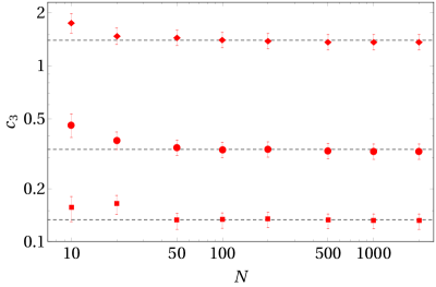
Figure 1: Finite size scaling for $c_{3}$. The plot shows the dependence on $N$ of the third moment of the correlation matrix. The data are obtained by the average over $50$ different realizations for each $N$ and $\alpha=0.1$ (red squares), $0.2$ (red circles) and $0.5$ (red diamonds). The dashed black lines are the relative $N\rightarrow\infty$ values of $c_{3}$ coming from the finite-size scaling analysis.

We now compare the theoretical outcomes predicted by the analytical expression of the quenched free energy (Disordered Statistical Mechanics) with the numerical estimations of the momenta of the correlation function (Random Matrix Theory).

Concerning the latter, on the numerical side, we consider 50 different realizations of the couplings $\boldsymbol{\xi}$ for $N=10,20,50,100,\dots,2000$ and $\alpha=0.1,0.2,\dots,0.9$, and then we compute the powers of correlation matrix (we restricted the inspection to the lowest orders $n=1,2,3,4,5$) and finally we average over the samples. For increasing $N$, at fixed $\alpha$, the momenta settle on their “thermodynamic” values. We therefore perform a finite-size scaling analysis by fitting numerical data for sufficiently large $N$: an example of this analysis is reported in Fig. 1 for the momenta $c_{3}$ for $\alpha=0.1,0.2,0.5$.

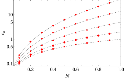
Figure 2: Comparison between theoretical predictions and numerical results. The plot shows the comparison between the numerical results (obtained with the finite-size scaling analysis for the correlation matrix momenta) and the theoretical prediction derived by the generating function (30), which are explicitly collected in (48). The error bars for numerical data are too small to be visualized in the plot (because of the logarithmic scale).

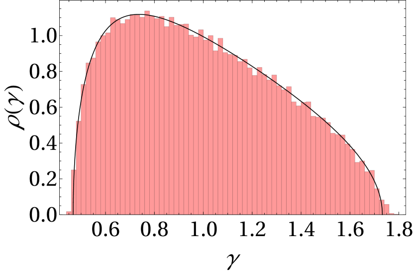
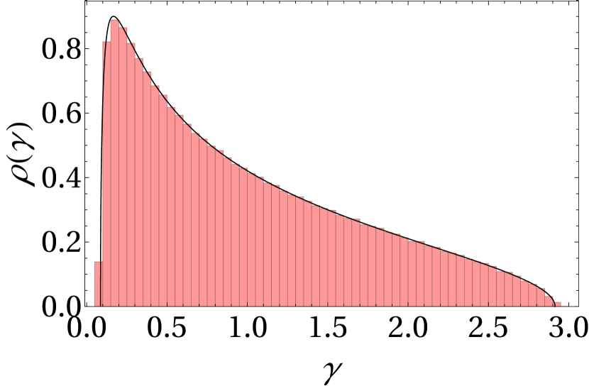
Figure 3: Spectral density versus frequency distributions. The plots show the eigenvalues histograms versus the spectral probability distribution (47). Numerical data are obtained from a sample of 200 correlation matrices with $N=1000$ and $\alpha=0.1$ (left plot) and $\alpha=0.5$ (right plot).

From the analytical side, by using both (39) and (30), we can easily determine the theoretical predictions for the correlation matrix momenta. For $n=1,\dots,5$, we easily find

$$\begin{split}c_{1}&=\alpha,\\ c_{2}&=\alpha(\alpha+1),\\ c_{3}&=\alpha\left(\alpha^{2}+3\alpha+1\right),\\ c_{4}&=\alpha(\alpha+1)\left(\alpha^{2}+5\alpha+1\right),\\ c_{5}&=\alpha\left(\alpha^{4}+10\alpha^{3}+20\alpha^{2}+10\alpha+1\right).\end{split}$$ (48)

The comparison between the numerical estimations and the theoretical predictions is reported in Fig. 2, showing a perfect agreement between the numerical data and the analytical solutions from the quenched free energy of the analog bi-partite spin-glass.

For the sake of completeness, we compare also the Marchenko-Pastur law (47) derived in our setup with numerical simulations. To do this, we considered a sample of $200$ correlation matrices with $N=1000$ and $\alpha=0.1,0.5$. Then, we computed the eigenvalues of each matrix in the sample and realize the histogram. The latter is compared with the spectral probability distribution according to Marchenko-Pastur law. Also in this case, it emerges a perfect agreement between numerical data and the analytical solution, as it emerges from Fig 3.

5 Conclusions

Bipartite spin-glasses bipartiti have recently attracted much attention (see e.g. Auffinger-bip ; Barra-Multispecies ; Gavin-bip ; Monasson and references therein) as they constitute the natural mathematical scaffold for Boltzmann machines Hinton1 ; HintonLast , the latter being the building blocks of powerful inferential architectures (e.g. the so-called deep Boltzmann machines Hugo ) in Machine Learning.
Bipartite spin-glasses can be equipped with binary or real valued spins and/or couplings and, as extensively revised in Barra-RBMsPriors1 ; Barra-RBMsPriors2 , a “quasi-universal” behavior emerges in these models (i.e. solely the retrieval properties are strongly sensible to the nature of these variables but the resulting structure of the quenched noise -coded in the overlaps- is unaffected by the details of the priors), a property share by random matrices, whose study lies in Random Matrix Theory.
In this work we focused on the fully analog bipartite spin-glass, namely a two-layer network whose layers (or parties) share standard Gaussian spins and also the (quenched) couplings among the spins are drawn from standard i.i.d. Gaussian distributions. The main route, in the disordered statistical mechanical analysis of the model, is to look for an explicit expression of quenched free energy related to the cost function defining the model, possibly in terms of the natural parameters of the theory, that -in the present case- turn out to be the self and two-replica overlaps, for each layer.
Confining our investigation to a replica symmetric scenario (that is however expected to be correct for these analog models gaussian-spinglass ; BenArous ), we obtained an explicit expression for the quenched free energy by using both the interpolation technique Barra-JSP2010 ; Guerra-Broken and the replica-trick MPV , finding overall perfect agreement among the outcomes of the two computations.
A remarkable property of this analog model is that it is entirely approachable even without the knowledge of statistical mechanical techniques (as, being the model entirely Gaussian it is mathematically tractable) and a direct calculation shows that the quenched free energy of this model is the generating functional for the momenta of the related Willshaw matrix (namely the correlation matrix among the weights, that -not by chance- turns out to be Hebbian Amit ; BarraEquivalenceRBMeAHN ; Coolen ): this novel bridge allows drawing a number of conclusions. In particular, we have shown here how -reversing the perspective- we can obtain information in Random Matrix Theory by using Statistical Mechanics: by applying the Stieltjes-Perron inversion formula on the quenched free energy of the analog bi-partite spin-glass the spectral density of the Wishart matrix (or Hebbian kernel) can be obtained in terms of the celebrated Marchenko-Pastur distribution.
These analytical findings have been also supported by extensive numerical simulations finding overall full agreement.

6 Acknowledgments

The Authors are grateful to Alessia Annibale and Reimer Kühn for useful discussions. The Authors acknowledge partial financial fundings by MIUR via FFABR2018-(Barra) and by INFN.

References

- (1) D.H. Ackley, G.E. Hinton, T.J. Sejnowski, A learning algorithm for Boltzmann machines, Cognitive Sci. 9.1:147-169, (1985).
- (2) E. Agliari, A. Barra, A. De Antoni, A. Galluzzi, Parallel retrieval of correlated patterns: From Hopfield networks to Boltzmann machines, Neur. Net. 38, 52, (2013).
- (3) E. Agliari, A. Barra, C. Longo, D. Tantari, Neural Networks retrieving binary patterns in a sea of real ones, J. Stat. Phys. 168, 1085, (2017).
- (4) E. Agliari, et al., Retrieval capabilities of hierarchical networks: From Dyson to Hopfield, Phys. Rev. Lett.s 114, 028103, (2015).
- (5) E. Agliari, et al., Multitasking associative networks, Phys. Rev. Lett. 109, 268101, (2012).
- (6) E. Agliari, et al, Immune networks: multitasking capabilities near saturation, J.Phys.A: Math. Theor. 46(41):415003, (2003).
- (7) D.J. Amit, Modeling brain functions, Cambridge Univ. Press (1989).
- (8) A. Auffinger, W.K. Chen, The Parisi formula has a unique minimizer, Comm. Math. Phys. 335.3:1429, (2015).
- (9) A. Auffinger, W.K. Chen, Free Energy and Comlexity of Sherical Biartite Models, J. Stat. Phys. 157.1:40, (2014).
- (10) J. Aukosh, I. Tobasco, A dynamic programming approach to the Parisi functional, Proc.s Am. Math. Soc. 144.7:3135, (2016).
- (11) F. Barahona, On the computational complexity of Ising spin glass models. J.Phys.A: Math. Gen. 15.10:3241, (1982).
- (12) A. Barra, Irreducible Free energy expansion and overlaps locking in mean field spin glasses, J. Stat. Phys. 123(3):601, (2006).
- (13) A. Barra, M. Beccaria, A. Fachechi,A new mechanical approach to handle generalized Hopfield neural networks, Neural Networks (2018).
- (14) A. Barra, et al., On the equivalence among Hopfield neural networks and restricted Boltzman machines, Neural Networks 34, 1-9, (2012).
- (15) A. Barra, F. Guerra, E. Mingione, Interpolating the Sherrington-Kirkpatrick replica trick, Phil. Magaz. 92, 78, (2011).
- (16) A. Barra, et al., Phase transitions of Restricted Boltzmann Machines with generic priors, Phys. Rev. E 96, 042156, (2017).
- (17) A. Barra, et al., Phase Diagram of Restricted Boltzmann Machines Generalized Hopfield Models, Phys. Rev. E 97, 022310, (2018).
- (18) A. Barra, et al., Multi-species mean field spin glasses: Rigorous results, Ann. Henri Poincarè 16(3):691, (2015).
- (19) A. Barra, G. Genovese, F. Guerra, The replica symmetric approximation of the analogical neural network, J. Stat. Phys. 140(4):784, (2010).
- (20) A. Barra, G. Genovese, F. Guerra, Equilibrium statistical mechanics of bipartite spin systems, J. Phys. A 44, 245002, (2011).
- (21) A. Barra, F. Guerra, G. Genovese, D.Tantari, How glassy are neural networks?, JSTAT P07009, (2012).
- (22) A. Barra, G. Genovese, F. Guerra, D. Tantari, A solvable mean field model of a gaussian spin glass, J.Phys.A: Math. Theor. 47, 155002, (2014).
- (23) G. Ben Arous, A. Dembo, A. Guionnet, Aging of spherical spin glasses, Prob. Theor. Rel. Fields 120, 1, (2001).
- (24) G. Biroli, J.P. Bouchaud, M. Potters, Extreme value problems in random matrix theory and other disordered systems, JSTAT P07019, (2007).
- (25) J.D. Bryngelson, P.G. Wolynes, Spin glasses and the statistical mechanics of protein folding, Proc. Natl. Acad. Sci. 84.21:7524, (1987).
- (26) D. Bollè, T.M. Nieuwenhuizen, I.P. Castillo, T. Verbeiren, A spherical Hopfield model, J.Phys.A: Math. Theor. 36(41):10269, (2003).
- (27) A. Bovier, Self-averaging in a class of generalized Hopfield models, J.Phys.A: Math. Theor. 27.21:7069, (1994).
- (28) A. Bovier, P. Picco, Mathematical aspects of spin glasses and neural networks, Springer Press (2012).
- (29) P. Carmona, Y. Hu, Universality in Sherrington–Kirkpatrick’s spin glass model, Ann. Henri Poincarè 42, 2, (2006).
- (30) A.C.C. Coolen, R. Kühn, P. Sollich, Theory of neural information processing systems, Oxford Press (2005).
- (31) V. Dotsenko, An introduction to the theory of spin glasses and neural networks, World Scientific, (1995).
- (32) A. Fachechi, E. Agliari, A. Barra, Dreaming neural networks: forgetting spurious memories and reinforcing pure ones, submitted to Neural Nets available at arXiv:1810.12217 (2018).
- (33) S. Galluccio, J.P. Bouchaud, M. Potters, Rational decisions, random matrices and spin glasses, Physica A: Stat. Mech. its Appl.s 259.3-4: 449, (1998).
- (34) E. Gardner, The space of interactions in neural network models, J. Phys. A 21(1):257, (1988).
- (35) H. Gavin, E. Parker, E. Geist, Replica Symmetry Breaking in Bipartite Spin Glasses and Neural Networks, arXiv preprint arXiv:1803.06442, (2018).
- (36) G. Genovese, Universality in bipartite mean field spin glasses, J. Math. Phys. 53.(12):123304, (2012).
- (37) G. Genovese, D. Tantari, Legendre duality of spherical and Gaussian spin glasses, Math. Phys., Analysis Geom. 18.1:10, (2015).
- (38) I. Goodfellow, Y. Bengio, A. Courville, Deep Learning, M.I.T. press (2017).
- (39) F. Guerra, The cavity method in the mean field spin glass model. Functional representations of thermodynamic variables, Adv. Dynam. Sys. Quant. Phys. (1995).
- (40) F. Guerra, Broken replica symmetry bounds in the mean field spin glass model, Comm. Math. Phys. 233:(1), 1-12, (2003).
- (41) J.J. Hopfield, Neural networks and physical systems with emergent collective computational abilities, Proceedings of the national academy of sciences 79.8 (1982): 2554-2558.
- (42) P.L. Hsu, On the distribution of roots of certain determinantal equations, Annals of Hum. Gen. 9(3):250, (1939).
- (43) E.T. Jaynes, Information theory and statistical mechanics, Phys. Rev. 106.4:620, (1957).
- (44) S. Kauffman, S. Levin, Towards a general theory of adaptive walks on rugged landscapes, J. Theor. Biol. 128.1:11-45, (1987).
- (45) A. Martirosyan , M. Figliuzzi, E. Marinari, A. De Martino, Probing the Limits to MicroRNA-Mediated Control of Gene Expression, Plos Comp. Biol. 12(1):e1004715, (2016).
- (46) V.A. Marchenko, L.A. Pastur, Distribution of eigenvalues for some sets of random matrices, Matematicheskii Sbornik 114(4):507-536, (1967).
- (47) M.L. Mehta, Random matrices, Elsevier (2004).
- (48) M. Mezard, Mean-field message-passing equations in the Hopfield model and its generalizations, Phys. Rev. E 95(2), 022117, (2017).
- (49) M. Mezard, G. Parisi, M.A. Virasoro, SK model: The replica solution without replicas, Europhys. Lett.s 1.2:77, (1986).
- (50) M. Mezard, G. Parisi, M.A. Virasoro, Spin glass theory and beyond: an introduction to the replica method and its applications, World Scientific, Singapore (1987)
- (51) M. Mezard, G. Parisi, R. Zecchina, Analytic and algorithmic solution of random satisfiability problems, Science 297.5582:812, (2002).
- (52) R. Monasson, et al., Determining computational complexity from characteristic ‘phase transitions’, Nature 400.6740:133, (1999).
- (53) H. Nishimori, Statistical physics of spin glasses and information processing: an introduction, Clarendon Press, (2001).
- (54) D. Panchenko, The Sherrington-Kirkpatrick model, Springer Press, (2013).
- (55) G. Parisi, Infinite number of order parameters for spin-glasses, Phys. Rev. Lett.s 43(23):1754, (1979).
- (56) G. Parisi, The order parameter for spin glasses: a function on the interval , J.Phys.A: Math. Gen. 13(3):1101, (1979).
- (57) G. Parisi, A sequence of approximated solutions to the SK model for spin glasses, J.Phys.A: Math. Gen. 13(4): L115, (1980).
- (58) G. Parisi, Asymmetric neural networks and the process of learning, J.Phys.A: Math. Gen. 19.11: L675, (1986).
- (59) G. Parisi, A simple model for the immune network, Proc. Natl. Acad. Sci. 87(1):429, (1990).
- (60) G. Parisi, On the classification of learning machines, Network: Comput. in Neur. Sys. 3.3:259, (1992).
- (61) L. Pastur, M. Shcherbina, B. Tirozzi, The replica-symmetric solution without replica trick for the Hopfield model, J. Stat. Phys. 74(5-6):1161, (1994).
- (62) L. Pastur, M. Shcherbina, B. Tirozzi, On the replica symmetric equations for the Hopfield model, J. Math. Phys. 40(8): 3930, (1999).
- (63) L. Peliti, Introduction to the statistical theory of Darwinian evolution, arXiv preprint cond-mat/9712027, (1997).
- (64) T. Rogers, I.P. Castillo, R. Kühn, K. Takeda, Cavity approach to the spectral density of sparse symmetric random matrices, Phys. Rev. E 78(3):031116, (2008).
- (65) R. Salakhutdinov, H. Larochelle, Efficient learning of deep Boltzmann machines, Proc. thirteenth int. conf. on artificial intelligence and statistics, 693, 2010.
- (66) R. Salakhutdinov, G. Hinton, Deep Boltzmann machines, Artificial Intelligence and Statistics (2009).
- (67) E. Schneidman, M.J. Berry II, R. Segev, M. Bialek, Weak pairwise correlations imply strongly correlated network states in a neural population Nature 440(7087):1007, (2006).
- (68) H.S. Seung, H. Sompolinsky, N. Tishby, Statistical mechanics of learning from examples, Phys. Rev. A 45(8):6056, (1992).
- (69) N. Srivastava, R. Salakhutdinov, Multimodal learning with deep boltzmann machines, Adv. Neural Inform. Proc. Sys. , 2222, (2012).
- (70) M. Talagrand, Spin glasses: a challenge for mathematicians: cavity and mean field models, Springer Science Business Media, (2003).
- (71) M. Talagrand, The Parisi formula, Annals of Mathematics, 221-263 (2003).
- (72) T. Tao, Topics in random matrix theory, American Mathematical Soc. 132, (2012).
- (73) J. Tubiana, R. Monasson, Emergence of Compositional Representations in Restricted Boltzmann Machines, Phys. Rev. Lett. 118.13:138301, (2017).
- (74) P. Vivo, S. N. Majumdar, O. Bohigas, Large deviations of the maximum eigenvalue in Wishart random matrices, J.Phys.A: Math. Theor. 40.16:4317, (2007).
- (75) R. Allez, J.P. Bouchaud, S.N. Majumdar, P. Vivo, Invariant -Wishart ensembles, crossover densities and asymptotic corrections to the Marcenko–Pastur law J.Phys.A: Math. Theor. 46(1):015001, (2012).
- (76) G. Parisi, A. Vulpiani, Scaling law for the maximum Lyapunov characteristic exponent of infinite product of random matrices, J.Phys.A: Math. Gen. 19(8):L425, (1986).
- (77) E.P. Wigner On the distribution of the roots of certain symmetric matrices, Annals of Math. 67(2):325, (1958).
- (78) J. Wishart, The generalised product moment distribution in samples from a normal multivariate population, Biometrika, 20A(1/2):32, 52, (1928).