On-sky performance of the CLASS Q-band telescope

tablenum SIXtablenum

1 Introduction

Mapping the polarization of the cosmic microwave background (CMB) is essential for understanding the earliest moments of the Universe. In addition to constraining inflation (Guth, 1981; Sato, 1981; Linde, 1982; Starobinsky, 1982; Albrecht & Steinhardt, 1982; Planck Collaboration et al., 2018c) and the standard six-parameter $\Lambda$CDM model (Hinshaw et al., 2013; Planck Collaboration et al., 2018b), the polarization of the CMB is a probe for the epoch of reionization and the growth of large-scale structure. The $100\text{\,}\mathrm{\SIUnitSymbolMicro K}$ CMB intensity fluctuations are polarized by Thomson scattering at the few percent level (Rees, 1968; Kovac et al., 2002). This polarization is decomposed into E modes, which provide our best constraint on the optical depth to reionization (Hinshaw et al., 2013; Planck Collaboration et al., 2018b), and B modes, which probe inflationary gravitational radiation (Kamionkowski et al., 1997; Zaldarriaga & Seljak, 1997). The B-mode component is at least ten times fainter than the E-mode component (BICEP2 Collaboration et al., 2018). Both must be separated from polarized Galactic emission (e.g. BICEP2 Collaboration et al. (2016)). Averaged over the sky at high galactic latitudes, polarized dust emission is the dominant Galactic component at frequencies above $70\text{\,}\mathrm{GHz}$ (Planck Collaboration et al., 2015, 2016b; Planck Collaboration Int. L, 2017; Planck Collaboration et al., 2018d), while synchrotron is the strongest polarized emission mechanism at lower frequencies (Planck Collaboration et al., 2018a; Bennett et al., 2013). On small angular scales gravitational lensing of E-modes induces a B-mode signal larger than the current upper limit on primordial inflationary B-modes. Efforts toward characterizing these small angular scale B-modes include Polarbear Collaboration et al. (2014), Henning et al. (2018), and Louis et al. (2017).

The Cosmology Large Angular Scale Surveyor (CLASS) will measure the polarized microwave sky in bands centered at approximately $40\text{\,}\mathrm{GHz}90\text{\,}\mathrm{GHz}150\text{\,}\mathrm{GHz}220\text{\,}\mathrm{GHz}$ from an altitude of $5200\text{\,}\mathrm{m}$ above sea level in the Atacama Desert of northern Chile (Essinger-Hileman et al., 2014; Harrington et al., 2016) inside the Parque Astronómico Atacama (Bustos et al., 2014). The Q-band ($40\text{\,}\mathrm{GHz}$) telescope probes synchrotron emission (Eimer et al., 2012; Appel et al., 2014), whereas the G-band (dichroic $150\text{\,}\mathrm{GHz}220\text{\,}\mathrm{GHz}$) telescope maps dust. Two W-band ($90\text{\,}\mathrm{GHz}$) telescopes provide the necessary sensitivity to the CMB polarized signal (Dahal et al., 2018). The location, design, and survey strategy of the CLASS telescopes are defined to reconstruct the microwave polarization at large angular scales (multipoles $2<\ell\lesssim 200$) over 75% of the sky. To achieve this goal, CLASS employs a Variable-delay Polarization Modulator (VPM) as its first optical element to increase stability and mitigate instrumental polarization (Miller et al., 2016; Chuss et al., 2012a). The benefits of implementing a fast ($\sim$$10\text{\,}\mathrm{Hz}$) polarization modulator as your first optical element has been demonstrated from the ground by the Atacama B-mode Search experiment (Kusaka et al., 2014, 2018). Telescope boresight rotation and a comoving ground shield mitigate contamination by terrestrial polarization sources. The CLASS survey is forecast to constrain the optical depth to reionization $\tau$ to near the cosmic variance limit and the inflationary tensor-to-scalar ratio to $r\approx 0.01$ (Watts et al., 2015, 2018). The optical depth is the least constrained $\Lambda$CDM parameter, and new measurements at $\ell<12$ are important for realizing the full potential of cosmological probes of neutrino masses (Allison et al., 2015; Watts et al., 2018).

This is the first paper describing the on-sky performance of CLASS. This analysis is based on observations with the CLASS Q-band telescope between June 2016 and March 2018 (see Figure 1). In this paper we discuss the calibration and performance of the Q-band telescope for intensity measurements, leaving discussions of polarized performance to future papers. In Section 2, we present median detector parameters extracted from $I$-$V$ measurements and array sensitivity estimates based on the power spectral density (PSD) of the time-ordered data (TOD). In Section 3, observations of the Moon are used to constrain the average detector beam, the relative gain between detectors, the telescope optical efficiency, and the calibration factor to convert power measured at the detectors to antenna temperature. Using this Moon-based antenna temperature calibration, we present a new measurement of Tau A flux density at Q band in Section 4. Finally, Section 5 summarizes the CLASS Q-band detector array performance during its first observing campaign.

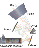
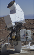
Figure 1: Left: Diagram of the Q-band instrument including baffle, VPM, mirrors, and cryostat  (Eimer et al., 2012; Essinger-Hileman et al., 2014; Appel et al., 2014; Harrington et al., 2016, 2018). For a closer view of the Q-band detector assembly and cryogenic receiver see: Figure 1 in Rostem et al. (2014b); Appel et al. (2014), and Figure 8 in Harrington et al. (2016). Right: Photograph of the Q-band telescope configuration during the June 2016 to March 2018 observing period. The telescope is enclosed in a metal structure that protects the instruments and prevents pickup from terrestrial sources.

2 On-sky detector characteristics

TES Bolometer Parameters
Phonon Power ($P_{\upvarphi}$)	$6.3\text{\,}\mathrm{pW}$
Bias Power ($P$)	$4.2\text{\,}\mathrm{pW}$
Dark Power Offset ($P_{\mathrm{D}}$)	$0.5\text{\,}\mathrm{pW}$
Optical Loading ($P_{\gamma}$)	$1.6\text{\,}\mathrm{pW}$
Responsivity ($S$)	$-8.2\text{\,}\mathrm{\SIUnitSymbolMicro A}\text{\,}{\mathrm{pW}}^{-1}$
Optical Time Constant ($\tau_{\gamma}$)	$3.4\text{\,}\mathrm{ms}$
Thermal Time Constant ($\tau_{\upvarphi}$)	$17\text{\,}\mathrm{ms}$
Heat Capacity ($C$)	$3\text{\,}\mathrm{pJ}\text{\,}{\mathrm{K}}^{-1}$
Thermal Conductivity ($G$)	$177\text{\,}\mathrm{pW}\text{\,}{\mathrm{K}}^{-1}$
Thermal Conductivity Constant ($\kappa$)	$13.4\text{\,}\mathrm{n}\mathrm{W}~{}\mathrm{K}^{-4}$
Critical Temperature ($T_{\mathrm{c}}$)	$149\text{\,}\mathrm{mK}$
Normal Resistance ($R_{\mathrm{N}}$)	$8.2\text{\,}\mathrm{m\SIUnitSymbolOhm}$
Shunt Resistance ($R_{\mathrm{sh}}$)	$0.25\text{\,}\mathrm{m\SIUnitSymbolOhm}$
TES loop Inductance ($L$)	$500\text{\,}\mathrm{nH}$

Optical Performance Parameters
System Noise Temperature (${T}_{\mathrm{sys}}$)	$27\text{\,}\mathrm{K}$
Telescope Efficiency ($\eta$)	0.48
RJ Temp Calibration ($\frac{dT_{\mathrm{RJ}}}{dP_{\gamma}}$)	$13.1\text{\,}\mathrm{K}\text{\,}{\mathrm{pW}}^{-1}$
CMB-RJ Calibration ($\frac{dT_{\mathrm{cmb}}}{dT_{\mathrm{RJ}}}$)	1.04
Detector Dark Noise Power ($\mathrm{NEP}_{\mathrm{d}}$)	$11\text{\,}\mathrm{a}\mathrm{W}\sqrt{\mathrm{s}}$
Detector Total Noise Power ($\mathrm{NEP}$)	$19\text{\,}\mathrm{a}\mathrm{W}\sqrt{\mathrm{s}}$
Detector Noise Temperature ($\mathrm{NET}$)	$258\text{\,}\mathrm{\SIUnitSymbolMicro}\mathrm{K}_{\mathrm{cmb}}\sqrt{\mathrm{s}}$
Optical Detectors ($N_{\mathrm{det}}$)	64
Array Noise Temperature	$32\text{\,}\mathrm{\SIUnitSymbolMicro}\mathrm{K}_{\mathrm{cmb}}\sqrt{\mathrm{s}}$
RJ Extended Source Band Center ($\nu_{\mathrm{o}}$)	$38.0\text{\,}\mathrm{GHz}$
RJ Point Source Band Center ($\nu^{\prime}_{\mathrm{o}}$)	$38.5\text{\,}\mathrm{GHz}$
Bandwidth ($\Delta\nu$)	$11.4\text{\,}\mathrm{GHz}$
Beam Solid Angle ($\Omega$)	$796\text{\,}\mathrm{\SIUnitSymbolMicro sr}$
RJ Point Source Flux Factor ($\Gamma$)	$27.6\text{\,}\mathrm{\SIUnitSymbolMicro K}\text{\,}{\mathrm{Jy}}^{-1}$

Table 1: Table of Q-band detector parameters. Parameters on the left column are derived with the help of $I$-$V$ data and represent the median value across the detector array. Time constant and heat capacity estimates also depend on measurements of the VPM synchronous signal. The right-hand side parameters are derived using: TOD power spectral density near the 10 Hz modulation frequency to estimate NEP, Moon observations to measure the beam solid angle and calibrate power at the bolometer to antenna temperature, and laboratory Fourier-Transform Spectrometer (FTS) measurements to determine bandpass properties.

The Q-band array consists of 36 feedhorn-coupled, dual-polarization detectors. Each polarimeter has two transition edge sensor (TES) bolometers, one for measuring the optical power in each orthogonal linear polarization channel (Appel et al., 2014; Rostem et al., 2012; Chuss et al., 2012b, 2014). The bolometers are read out through time-division multiplexing (TDM) of superconducting quantum interference device (SQUID) amplifiers (Doriese et al., 2016; Battistelli et al., 2008). The CLASS Q-band two-stage TDM scheme consists of $8$ columns multiplexing $11$ rows of SQUIDs, for a total of $88$ channels, of which $14$ are dedicated dark SQUID channels used to characterize readout noise and magnetic field pickup. A dark SQUID is a readout channel that is not connected to a TES bolometer. Two readout channels are connected to dark TES bolometers fabricated within the polarimeter chips (Denis et al., 2009, 2016). Unlike the optical bolometers, the dark bolometers are not connected to antennas at the waveguide output of the feedhorns (Chuss et al., 2012b; Ade et al., 2009). Of the $72$ polarization sensitive bolometers, 64 were operational during the first observing campaign; the remaining eight channels were lost during deployment due to a readout electronics failure. These channels were recovered for the second observing campaign, which began in June 2018.

The Q-band telescope observed on a 24-hour cycle that started routinely at 14:00 UTC (late-morning local time). The Q-band receiver operates a dilution refrigerator that continuously cools the detector array to $T_{\mathrm{b}}\approx$42\text{\,}\mathrm{mK}$$ (Iuliano et al., 2018) during science operations, therefore allowing any observation cadence. Our 24 hour cycle is chosen to yield a full sky map each day at one boresight. We change boresight angle everyday, and the timing of the schedule end/start coincides with the site crew work schedule. At the beginning and end of an observation cycle, the detector bias voltage ($V$) was swept while recording the current response ($I$) to produce what will hereafter be called an “$I$-$V$ curve.” Additional $I$-$V$ curves are acquired before special data sets such as wire-grid calibration measurements, and detector noise tests with the cryostat window covered. These $I$-$V$ curves are used to choose the optimal bias voltage for each column composed of up to 10 TES bolometers. During observations these bias voltages place the array TES bolometers on their superconducting transition between 30% and 60% of their normal resistance. The detector saturation power ($P_{\mathrm{sat}}$) is extracted from $I$-$V$ data and defined as the detector bias power ($P=IV$) evaluated at 80% of the TES normal resistance ($R_{\mathrm{N}}$). The difference between the $P_{\mathrm{sat}}$ measured in dark laboratory tests with the detectors enclosed in a $1\text{\,}\mathrm{K}$ cavity ($P_{\upvarphi}$), and those measured while observing the sky is interpreted as the optical power loading ($P_{\gamma}$) on the detectors. Included in this number is a correction for a small offset tracked by neighboring nonoptical bolometers ($P_{\mathrm{D}}$) discussed in section 2.1.

Detector responsivity ($S=\mathrm{d}I/\mathrm{d}P_{\gamma}$) estimated from $I$-$V$ data is used to calibrate current signals ($\mathrm{d}I$) across the TES to power deposited on the bolometer ($\mathrm{d}P_{\gamma}$). Detector optical time constants are extracted from the delayed response to the VPM synchronous signal (see Figure 2) that appears at the modulation frequency of $10\text{\,}\mathrm{Hz}$. Combining measured time constants with $I$-$V$ curve data, we derive the heat capacity of the bolometers. Table 2 summarizes median detector parameters across the array during this period.

2.1 Optical loading

Figure 2: Left: The blue solid line shows the array-averaged radial beam profile derived from Moon observations, and the gray shaded region the measurement uncertainty. The main lobe is similar to a 1.5 degree Gaussian beam. The black line shows the array-averaged beam solid angle versus radius with a total solid angle of $796\text{\,}\mathrm{\SIUnitSymbolMicro sr}$ (Xu et al., in prep.). Center: The solid line plots the simulated detector bandpass (Chuss et al., 2012b) with center frequency $38.0\text{\,}\mathrm{GHz}$ and bandwidth $11.4\text{\,}\mathrm{GHz}$. The connected dots show a Q-band detector bandpass extracted from fourier transform spectrometer (FTS) measurements made in the laboratory (see Dahal et al. (2018) for a description of the FTS testing setup). We use a Martin-Puplett FTS (T. Wei 2010, private communication; Martin & Puplett, 1970) with a liquid nitrogen cooled blackbody (Petroff et al., 2019) as the input source while the FTS output is directed at a CLASS feedhorn coupled Q-band bolometer placed one meter behind a ten centimeter diameter cold stop. The feedhorn’s frequency dependent gain (Zeng, 2012) and the transmission of the lab-cryostat filters are divided out from the raw FTS measurement. The center frequency of the measured bandpass matches the simulation and has an estimated uncertainty of $0.2\text{\,}\mathrm{GHz}$ driven by the lab-cryostat filter transmission model. The $\sim$1\text{\,}\mathrm{GHz}$$ resolution of the FTS broadens the measured bandpass edges compared to the simulation. The remaining differences between the measured and simulated bandpass are likely due to unaccounted systematics of the FTS and/or the coupling optics. The detector bandpass corresponds to the effective telescope bandpass for a beam filling extended Rayleigh-Jeans (RJ) thermal source. The effective center frequency for a Rayleigh-Jeans point source is $38.5\text{\,}\mathrm{GHz}$, obtained from combining the detector bandpass with the telescope frequency dependent gain (Fluxa, in prep.). Right: The raw (black) and time-constant corrected (blue) detector response to the VPM synchronous signal binned with respect to the grid-mirror distance (Harrington et al., in prep.). The black arrows indicate the direction of the raw signal as the VPM mirror is moved.

The in-band (see bandpass in Figure 2) optical power $P_{\gamma}$ dissipated on each bolometer is equal to the difference between the on-sky detector bias power $P$ and the phonon power $P_{\upvarphi}$ that flows from the bolometer island to the bath:

$$P_{\gamma}=P_{\upvarphi}-P,$$ (1)

where $P_{\upvarphi}$ and the bias power $P$ are both measured with the detector baseplate temperature at $T_{\mathrm{b}}\approx$50\text{\,}\mathrm{mK}$$ ($P_{\upvarphi}$ is equivalent to $P_{\mathrm{sat}}$ measured in dark laboratory tests with no optical loading). The detector copper baseplate serves as both mechanical support and thermal heatsink for the detector chips (Appel et al., 2014). Its temperature is tracked by a calibrated ruthenium oxide (ROX) temperature sensor.

The Q-band array contains two dark TES bolometers that have similar electro-thermal properties to the optical detectors in the array, but are disconnected from the on-chip planar microwave circuitry that couples the radiation from a feedhorn to the optical TES bolometers in a pixel. The saturation power for these bolometers decreases on average by $P_{\mathrm{D}}=0.5~{}$pW when opening the $1\text{\,}\mathrm{K}$ detector cryostat volume to the sky. Daily changes in atmospheric conditions affect both $P$ for optical detectors as well as $P_{\mathrm{D}}$. In particular, we find that averaged across the observing period $P_{\mathrm{D}}/(P_{\upvarphi}-P)=0.26$. The dark detector response to scanning an unresolved source like the Moon is $<$0.03% that of the average optical detector. Hence the change in dark detector saturation power can be interpreted as an offset in $T_{\mathrm{b}}$ between the ROX and the silicon frame holding the bolometers, as opposed to optical coupling. This offset can be driven by changes in the $1\text{\,}\mathrm{K}$ nylon filter (Essinger-Hileman et al., 2014; Iuliano et al., 2018) temperature ($\sim$$4\text{\,}\mathrm{K}$ at its center) as atmospheric conditions change, since radiation emitted by the filter would fill the focal plane volume and weakly couple to the detector chip and/or the ROX. We find less likely the alternative explanation of out-of-band power coupling directly to the TES island due to careful detector design isolating the TES bolometers from possible light leaks, and the lack of any out-of-band signal in our FTS measurements. We assume dark detector saturation power offset is similar for all bolometers in the array; hence we subtract $P_{\mathrm{D}}$ from $P_{\gamma}$ for all optical channels.

The median in-band optical loading $P_{\gamma}=$1.6\text{\,}\mathrm{pW}$$ is consistent with the model presented in Essinger-Hileman et al. (2014) and Appel et al. (2014). Two factors deviate from the model: (1) slightly lower optical efficiency in the field reduces $P_{\gamma}$, and (2) the instrument’s baffle and mount enclosure structure source $0.2~{}$pW of additional optical power.

2.2 Detector responsivities and time constants

Ninety-eight percent of $I$-$V$ derived detector responsivities across all CMB observations fall between $5\text{\,}\mathrm{\SIUnitSymbolMicro A}\text{\,}{\mathrm{pW}}^{-1}13\text{\,}\mathrm{\SIUnitSymbolMicro A}\text{\,}{\mathrm{pW}}^{-1}$. This well-defined range is due to stable atmospheric loading, stable cryogenic temperatures, and near-optimal detector saturation powers (Rostem et al., 2014a).

The VPM consists of a wire-grid that is placed in front of a mirror. The millimeter spacing between the mirror and the grid is optimized for the Q-band telescope (Harrington et al., 2018). In the CLASS telescopes, the mirror position is modulated at a frequency of $10\text{\,}\mathrm{Hz}$ to achieve polarization modulation. In addition to reflecting and modulating the polarized sky signal, the VPM emits a small signal synchronous with the grid-mirror distance. Each subset of CMB time-ordered data is fitted for a detector time constant that minimizes the hysteresis of this synchronous signal sourced by the VPM (see Figure 2). Eighty-six percent of CMB scans yield detector time constant ($\tau_{\gamma}$) measurements between $2\text{\,}\mathrm{ms}6\text{\,}\mathrm{ms}$. All are short enough to respond to the targeted 10 Hz modulation frequency and several of its harmonics. Multiplying $\tau_{\gamma}$ by the electro-thermal feedback (Irwin & Hilton, 2005) speed-up factor estimated from $I$-$V$ data yields the detector thermal time constant ($\tau_{\upvarphi}$). The heat capacity ($C$) of each detector is then obtained by multiplying its average thermal time constant by the detector thermal conductivity ($G$). The measured average bolometer heat capacity is $3\text{\,}\mathrm{pJ}\text{\,}{\mathrm{K}}^{-1}$. All detector heat capacities are within $1\text{\,}\mathrm{pJ}\text{\,}{\mathrm{K}}^{-1}$ of the mean. Achieving the targeted heat capacity allows for stable/optimal biasing of the detectors in the field, improving detector sensitivity and observing efficiency.

2.3 Detector Noise

Detector noise performance is quantified in terms of noise equivalent power (NEP) at the bolometer. We measure the NEP by averaging the power spectral density of the detector output in the side bands of the 10 Hz modulation frequency (9–11 Hz). To reduce correlated noise and improve the white noise estimate, we calculate individual detector NEP by first subtracting the TOD of detector pairs within a pixel (coupled to a feedhorn), then computing the power spectral density of the pair difference TOD and dividing by a factor of two in power squared units. Here we do not consider single detectors whose pair is not operational; hence this NEP analysis focuses on 27 detector pairs.

The median single detector NEP in the first observing season is $\mathrm{NEP}=$19\text{\,}\mathrm{a}\mathrm{W}\sqrt{\mathrm{s}}$$. This result is consistent with expectations once we correct the design estimates in Essinger-Hileman et al. (2014) to account for photon bunching noise cross-terms, lower achieved optical efficiency, and additional beam spill onto the baffle and telescope enclosure structure. Optical loading on the bolometers varies with atmospheric conditions; this allows us to probe the detector $\mathrm{NEP}$ vs. $P_{\gamma}$ relationship. Each $I$-$V$ measurement yields a $P_{\gamma}$ estimate for each detector, which corresponds to the $\mathrm{NEP}$ measured in the subsequent time-ordered data acquisition. We find that the change in $P_{\gamma}$ and $\mathrm{NEP}$ between consecutive $I$-$V$ measurements is small.

The NEP of a bolometer observing blackbody radiation is subject to both dark detector noise ($\mathrm{NEP}_{\mathrm{d}}$) and photon noise ($\mathrm{NEP}_{\gamma}$). For the CLASS TES bolometers, $\mathrm{NEP}_{\mathrm{d}}$ is dominated by phonon thermal fluctuations but also contains contributions from TES Johnson noise and SQUID readout noise. Tests in dark laboratory cryostats yield an average Q-band array $\mathrm{NEP}_{\mathrm{d}}=$11\text{\,}\mathrm{a}\mathrm{W}\sqrt{\mathrm{s}}$$ (Appel et al., 2014).

The statistical properties of the photons emitted by thermal sources we observe (atmosphere, CMB, dielectric filters, Moon, etc.) generate noise fluctuations at the detector output, which cannot be suppressed by improving the detector characteristics (Richards, 1994; Zmuidzinas, 2003; van Vliet, 1967; Mather, 1982). The average variance in the number of photons ($n$) per mode sourced by a blackbody at temperature $T$ is $\langle(\Delta n)^{2}\rangle=\langle n\rangle+\langle n\rangle^{2}$. The first term indicates the blackbody photons obey Poisson statistics in the limit that $n~{}\ll 1$ ($kT/h\nu\ll 1$), while in the limit $n~{}\gg 1$ ($kT/h\nu\gg 1$), the second term dominates and the photons arrive in bunches. Here $k$ is Boltzmann’s constant and $h$ is Planck’s constant. Photon counting statistics are translated to NEP ($\mathrm{NEP}_{\gamma}$) by identifying the spectral power density observed through a single mode detector as $P_{\nu}=h\nu\langle n\rangle$; therefore (Richards, 1994):

$$(\mathrm{NEP}_{\gamma})^{2}=\int h\nu P_{\nu}d\nu+\int P_{\nu}^{2}d\nu\quad[$\text{\,}{\mathrm{W}}^{2}\text{\,}\mathrm{s}$],$$ (2)

where $\int P_{\nu}d\nu=P_{\gamma}\approx P_{\nu_{\mathrm{o}}}\Delta\nu\approx\eta kT\Delta\nu$ (since the CMB and other sources CLASS Q-band observes are close to the Rayleigh-Jeans limit), $\Delta\nu$ is the microwave signal bandwidth, and $\eta$ is the optical efficiency of the entire telescope system, including attenuation, reflection, and beam spill due to the detector, filters, lenses, window, mirrors, VPM, and baffle.

The total detector $\mathrm{NEP}$ can be expressed in terms of measured quantities $\mathrm{NEP}_{\mathrm{d}}$, $P_{\gamma}$, $\Delta\nu$, and detector band center frequency $\nu_{\mathrm{o}}$ as:

$$(\mathrm{NEP})^{2}=(\mathrm{NEP}_{\mathrm{d}})^{2}+h\nu_{\mathrm{o}}P_{\gamma}+\frac{P_{\gamma}^{2}}{\Delta\nu}\quad[$\text{\,}{\mathrm{W}}^{2}\text{\,}\mathrm{s}$].$$ (3)

Figure 3 shows the measured $\mathrm{NEP}$ on the $y$-axis, and on the $x$-axis the corresponding measured $P_{\gamma}$. Equation 3 is fitted to the data points by setting $\nu_{\mathrm{o}}=$ $38.0\text{\,}\mathrm{GHz}$ and leaving $\mathrm{NEP}_{\mathrm{d}}$ and $\Delta\nu$ as free parameters. The best fit result of $\mathrm{NEP}_{\mathrm{d}}=$10.5\pm 1.0\text{\,}\mathrm{a}\mathrm{W}\sqrt{\mathrm{s}}$$ and $\Delta\nu=$10.6\pm 0.9\text{\,}\mathrm{GHz}$$ is consistent with independent measurements of $11\text{\,}\mathrm{a}\mathrm{W}\sqrt{\mathrm{s}}$ and $11.4\text{\,}\mathrm{GHz}$. This confirms that the CLASS Q-band detectors are photon noise limited and that the NEP is dominated by the photon noise bunching term. This NEP model provides a quantitative understanding of possible sensitivity improvements to the instrument if optical loading can be reduced without decreasing optical efficiency. In particular, $300\text{\,}\mathrm{K}$ baffling configurations will be explored in future seasons, where control of systematic effects due to beam spill can be traded for sensitivity.

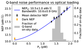
Figure 3: The histogram in the figure shows the Q-band optical loading distribution during observations. The relatively narrow range highlights the stability of the atmosphere at the CLASS site in the Atacama Desert of Chile. The black data points are the average NEP across the detector array for each bin of optical loading. The line is a model of on-sky NEP based on equation 3 with the center frequency set to $\nu_{\mathrm{o}}=$38.0\text{\,}\mathrm{GHz}$$, and the bandwidth $\Delta\nu$ and dark detector $\mathrm{NEP}_{\mathrm{d}}$ left as free parameters to fit. The results of the fit are consistent with independent FTS and dark laboratory measurements of $\Delta\nu$ and $\mathrm{NEP}_{\mathrm{d}}$ (see Table 2). The measured $\mathrm{NEP}_{\mathrm{d}}$ is plotted in orange at zero optical loading. Q-band $\mathrm{NEP}$ is dominated by bunching noise; therefore, sensitivity is driven by total optical loading and detector bandwidth. The model provides a quantitative prediction of instrument sensitivity as optical loading changes with the telescope design.

3 Moon observations and calibration to antenna temperature

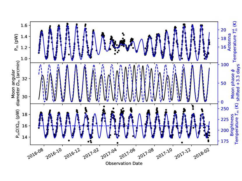
Figure 4: Top: Data points are the array-averaged peak Moon power measured at the bolometers ($P_{\mathrm{m}}$) across the observing period. The solid line is a model of the Moon’s antenna temperature based on the CLASS Q-band beam solid angle, the Moon’s time-dependent angular diameter, the Moon’s temperature oscillations that follow its phase, and an absolute calibration to a mean Moon temperature of $210\text{\,}\mathrm{K}$ at $38.5\text{\,}\mathrm{GHz}$ (Krotikov & Pelyushenko, 1987). Middle: The solid line plots the Moon’s angular diameter over time. The 27-day elliptical Moon orbit around the Earth is perturbed by the Sun. The dashed line plots the Moon phase delayed by 3.3 days to compensate for the measured lag in Moon brightness temperature. The 27-day orbital period and 29.5-day phase period interact to create the beat pattern observed in the top panel. Bottom: Data points from the top panel are divided by the beam-Moon dilution factor ($\eta_{\mathrm{m}}=\Omega_{\mathrm{m}}/\Omega^{\prime}$). The solid line plots the Moon’s brightness temperature model described by equation 5, with its parameters calibrated to match a mean temperature of $210\text{\,}\mathrm{K}$ marked with the dashed line. Differences between the data points and the model may be the result of weather, instrumental systematics, and/or limitations of the Moon emission model. Future work will explore implementing additional data quality tools and introducing a more complex Moon thermal model.

The electrical current signal from each TES detector is calibrated to power deposited on its bolometer island through responsivity estimates from the most recent $I$-$V$ acquisition. For the entire array, we find one calibration factor ($\mathrm{d}T_{\mathrm{RJ}}/\mathrm{d}P_{\gamma}$) from power deposited at the bolometer ($\mathrm{d}P_{\gamma}$) to antenna (Rayleigh-Jeans) temperature ($\mathrm{d}T_{\mathrm{RJ}}$) on the sky. At $38.0~{}\mbox{GHz}$, the conversion factor from $\mathrm{d}T_{\mathrm{RJ}}$ to CMB thermodynamic temperature ($\mathrm{d}T_{\mathrm{cmb}}$) is $\mathrm{d}T_{\mathrm{cmb}}/\mathrm{d}T_{\mathrm{RJ}}~{}=~{}1.04$. Individual detector TODs are calibrated to the array standard (i.e., the average) through a relative calibration factor $\epsilon_{j}$ equivalent to the inverse relative optical efficiency of the detector. Hence a small $\mathrm{d}I_{j}$ signal of detector $j$ is calibrated to $\mathrm{d}T_{\mathrm{cmb}}$ units through

$$dT_{\mathrm{cmb}}=\epsilon_{j}\frac{\mathrm{d}T_{\mathrm{cmb}}}{\mathrm{d}T_{\mathrm{RJ}}}\frac{\mathrm{d}T_{\mathrm{RJ}}}{\mathrm{d}P_{\gamma}}\frac{\mathrm{d}I_{j}}{S^{k}_{j}},$$ (4)

where $k$ identifies the $I$-$V$ used to estimate the detector responsivity $S^{k}_{j}$.

The Moon is an excellent target to constrain the absolute and relative calibrations of the CLASS Q-band detectors. At radio and millimeter wavelengths, the Moon radiates like a gray body, with frequency-dependent brightness temperature established by the optical depth of the lunar regolith and its thermal properties (Linsky, 1966; Troitskii, 1967). Unlike visible light, the scattering of microwave radiation from the Sun off the Moon’s surface is negligible compared to its thermal emission.

The Moon’s angular size of half a degree and $\sim$200\text{\,}\mathrm{K}$$ temperature at Q band approximates a point source for the 1.5 degree CLASS beam. When aligned with the beam center, the array-averaged peak Moon power measured at the bolometers is $P_{\mathrm{m}}\sim$1.3\text{\,}\mathrm{pW}$$, which is one-third of the average detector saturation power. The TES response is linear throughout the full range of the Moon signal, and a signal-to-noise ratio of $\sim$100\,000$$ is achieved. This allows the measurement of detector pointing, beams, and calibration factors from the nominal 720^∘ azimuth scan data whenever the Moon is in the field of view, increasing the observing efficiency by reducing time spent conducting targeted scans.

The absolute and relative detector calibrations extracted from Moon observations depend on the size of the average detector beam (see Figure 2) and the angular extent and brightness temperature of the Moon ($T_{\mathrm{m}}$) at $38.5\text{\,}\mathrm{GHz}$ on the date of observation. Moon-centered maps indicate the average detector beam matches the full width at half maximum (FWHM) design target of 1.5 degrees (see Figure 2). The average Moon angular diameter ($D_{\mathrm{m}}$) of 31 arc-minutes corresponds to a beam power dilution factor ($\eta_{\mathrm{m}}$) given by the ratio of the moon solid angle ($\Omega_{\mathrm{m}}$) to the solid angle of the convolution of the beam with the moon ($\Omega^{\prime}$), $\eta_{\mathrm{m}}=\Omega_{m}/\Omega^{\prime}=$ 0.077. This dilution factor makes the peak Moon antenna temperature $T^{A}_{\mathrm{m}}=\eta_{\mathrm{m}}T_{\mathrm{m}}\sim$$16\text{\,}\mathrm{K}$.

Tidal locking of the Moon’s rotation and its orbit results in one hemisphere of the Moon always facing the Earth. The Moon’s brightness temperature averaged across its Earth-facing hemisphere and across the lunar cycle ($\overline{T}_{\mathrm{m}}$) has been accurately measured at Q band with the aid of an “artificial Moon” calibrator (Krotikov & Troitskiĭ, 1964; Troitsky et al., 1968; Troitskii & Tikhonova, 1970; Krotikov & Pelyushenko, 1987). At $35\text{\,}\mathrm{GHz}$, Krotikov & Pelyushenko (1987) reports $\overline{T}_{\mathrm{m}}=$211\pm 5\text{\,}\mathrm{K}$$, and at $44\text{\,}\mathrm{GHz}$, $\overline{T}_{\mathrm{m}}=$208\pm 5\text{\,}\mathrm{K}$$. For the CLASS $38.5\text{\,}\mathrm{GHz}$ center frequency, we take $\overline{T}_{\mathrm{m}}=$210\pm 5\text{\,}\mathrm{K}$$. Linsky (1973) proposed using the brightness temperature at the center of the lunar disk as a radiometric standard for wavelengths between $10\text{\,}\mathrm{\SIUnitSymbolMicro m}$ and $1\text{\,}\mathrm{m}$. Near $8\text{\,}\mathrm{mm}$ wavelengths, Linsky (1973) estimates a time-averaged brightness temperature at the center of the lunar disk of $\sim$230\text{\,}\mathrm{K}$$. Note that the brightness temperature averaged across the entire lunar disk is lower than at the center due to colder temperatures near the poles. More recently, the ChangE satellite (Zheng et al., 2012) mapped the Moon temperature at $37\text{\,}\mathrm{GHz}$ with high resolution; unfortunately, the absolute calibration is less reliable due to beam side-lobe pickup of the cold antenna reference (Hu et al., 2017; Tsang et al., 2016).

The temperature of the Moon’s Earth-facing hemisphere oscillates with the fraction of Sun illumination or Moon phase (see bottom panel of Figure 4). At Q band, the maximum $T_{\mathrm{m}}$ peaks a few days after full Moon due to the heat capacity and thermal conductivity of the Moon’s surface material (Troitskii, 1967). The Moon phase follows on average a 29.53-day cycle, while the Moon orbital period is 27.32 days. The Moon’s elliptical orbit around Earth (strongly perturbed by the Sun) changes its angular diameter $D_{\mathrm{m}}$ on the sky, as shown in the middle panel of Figure 4. The two distinct periods of the Moon’s temperature and angular diameter oscillations cause a beat pattern in the measured antenna temperature ($T^{A}_{\mathrm{m}}$, see top panel of Figure 4). For example, in May 2017 the peak $T_{\mathrm{m}}$ coincided with minimum $D_{\mathrm{m}}$, nulling the fluctuation in $T^{A}_{\mathrm{m}}$, while the opposite effect occurred in November 2016 and December 2017.

To isolate the $T_{\mathrm{m}}$ oscillation from the Moon angular size variations, the $P_{\mathrm{m}}$ measurements across the observing era are divided by the time-dependent beam-Moon dilution factor $\eta_{\mathrm{m}}$: $P^{\prime}_{\mathrm{m}}=P_{\mathrm{m}}/\eta_{\mathrm{m}}$. $P^{\prime}_{\mathrm{m}}$ data points are fit to a simple sinusoidal model over time $t$:

$$P^{\prime}_{\mathrm{m}}=P^{\prime}_{0}+P^{\prime}_{1}\cos{(2\pi t/t_{\mathrm{o}}+\phi)},$$ (5)

where $P^{\prime}_{0}$ is the average brightness, $P^{\prime}_{1}$ is the amplitude of the brightness fluctuations, $t_{\mathrm{o}}$ the period of the oscillation, and $\phi$ the offset from full Moon. As expected, the fit yields $t_{\mathrm{o}}=29.5$ days, the same as the Moon phase period, and $\phi=3.3$ days after full Moon, indicating a lag between full Moon illumination and maximum brightness temperature. $P^{\prime}_{0}$ equals $16.0\text{\,}\mathrm{pW}$, and $P^{\prime}_{1}$ equals $2.2\text{\,}\mathrm{pW}$ (see bottom panel of Figure 4).

The Moon disk blocks the CMB radiation behind it; therefore $P^{\prime}_{\mathrm{m}}$ measures the difference between $T_{\mathrm{m}}$ and the background CMB brightness temperature at $38.0\text{\,}\mathrm{GHz}$, $T^{B}_{\mathrm{cmb}}=$1.9\text{\,}\mathrm{K}$$. $T^{B}_{\mathrm{cmb}}$ is less than the CMB’s blackbody temperature $T_{\mathrm{cmb}}=$2.725\text{\,}\mathrm{K}$$ (Fixsen, 2009) due to the brightness temperature definition, which is based on the Rayleigh-Jeans approximation. The CMB temperature was not known when the “artificial moon” observations were made; therefore we interpret their reported average Moon temperature to be measured with respect to the CMB background : $\overline{T}_{\mathrm{m}}=\langle{T}_{\mathrm{m}}-T^{B}_{\mathrm{cmb}}\rangle$. Note that the background CMB brightness temperature is less than 1% (and well within the uncertainty) of $\overline{T}_{\mathrm{m}}$.

The array’s absolute calibration factor is given by the ratio of the reported average Moon brightness temperature $\overline{T}_{\mathrm{m}}$ and the array-averaged brightness power $P^{\prime}_{0}$:

$$\frac{\mathrm{d}T_{\mathrm{RJ}}}{\mathrm{d}P_{\gamma}}=\frac{\overline{T}_{\mathrm{m}}}{P^{\prime}_{0}}=$13.1\pm 0.3\text{\,}\mathrm{K}\text{\,}{\mathrm{pW}}^{-1}$,~{}\mathrm{and}$$ (6)

$$\frac{\mathrm{d}T_{\mathrm{cmb}}}{\mathrm{d}P_{\gamma}}=\frac{\overline{T}_{\mathrm{m}}}{P^{\prime}_{0}}\frac{\mathrm{d}T_{\mathrm{cmb}}}{\mathrm{d}T_{\mathrm{RJ}}}~{}=~{}$13.6\pm 0.3\text{\,}\mathrm{K}\text{\,}{\mathrm{pW}}^{-1}$.$$ (7)

This absolute calibration factor translates to a telescope optical efficiency of:

$$\eta=\left(k\Delta\nu\frac{\mathrm{d}T_{\mathrm{RJ}}}{\mathrm{d}P_{\gamma}}\right)^{-1}=$0.48\pm 0.02$,$$ (8)

where the uncertainty on $\eta$ is driven by the uncertainty on $\Delta\nu$ ($\sigma_{\Delta\nu}=$0.5\text{\,}\mathrm{GHz}$$).

Relative calibration factors $\epsilon_{j}$ between detectors are obtained by dividing the array average Moon amplitude by the individual bolometer Moon measurement. These relative factors account for small differences in beam solid angle, bandpass, and optical efficiency across the detector array. Moon data indicate these are constant throughout the observing period and fall between 0.9 and 1.1.

The $\mathrm{NEP}$ noise measurements are multiplied by $\mathrm{d}T_{\mathrm{cmb}}/\mathrm{d}P_{\gamma}$ to obtain median single detector $\mathrm{NET}=$258\text{\,}\mathrm{\SIUnitSymbolMicro}\mathrm{K}_{\mathrm{cmb}}\sqrt{\mathrm{s}}$$. The average $P_{\gamma}=$1.6\text{\,}\mathrm{pW}$$ is equivalent to an antenna temperature of $T_{\gamma}~{}=P_{\gamma}/(\eta k\Delta\nu)~{}=~{}$21\text{\,}\mathrm{K}$$. We estimate that $5\text{\,}\mathrm{K}$ is from emission or spill within the cryostat (Iuliano et al., 2018) ($1\text{\,}\mathrm{K}$, $4\text{\,}\mathrm{K}$, and $60\text{\,}\mathrm{K}$ filters and lenses; $4\text{\,}\mathrm{K}$ cold stop; and $300\text{\,}\mathrm{K}$ filters and window), $6\text{\,}\mathrm{K}$ originates from the rest of the telescope (mirrors, VPM, closeout, mount enclosure, and baffle), $8\text{\,}\mathrm{K}$ comes from atmospheric emission, and $1.9\text{\,}\mathrm{K}$ from the CMB. The system noise temperature, $T_{\mathrm{sys}}=\mathrm{NEP}/\eta k\sqrt{\Delta\nu}=$27\text{\,}\mathrm{K}$$, implies an effective detector noise temperature of $T_{\mathrm{det}}=T_{\mathrm{sys}}-T_{\gamma}=$6\text{\,}\mathrm{K}$$.

4 Tau A intensity at Q band

Instrument	Year	$\nu_{e}$ ($\text{\,}\mathrm{GHz}$)	Flux ($\text{\,}\mathrm{Jy}$)	Flux 2017 ($\text{\,}\mathrm{Jy}$)	Flux 2017 at $38.4\text{\,}\mathrm{GHz}$ ($\text{\,}\mathrm{Jy}$)	References
NRL	1966	31.4	$387\pm 87$	$344\pm 77$	$321\pm 73$	Hobbs et al. (1968)
AFCRL	1967	34.9	$340^{+65}_{-40}$	$303^{+58}_{-36}$	$293^{+57}_{-36}$	Kalaghan & Wulfsberg (1967)
CBI	2000	31	$355.3\pm 18$	$341.7\pm 17$	$317\pm 19$	Cartwright et al. (2005); Cartwright (2003)
VSA	2001	33	$322\pm 4$	$310\pm 4$	$294\pm 11$	Hafez et al. (2008)
WMAP	2005	32.96	$342.8\pm 6.4$	$333.5\pm 6.2$	$316\pm 12$	Weiland et al. (2011)
WMAP	2005	40.64	$317.7\pm 8.6$	$307.9\pm 8.4$	$314\pm 13$	Weiland et al. (2011)
Planck	2011	30	$344.23\pm 0.27$	$339.51\pm 0.34$	$311\pm 10$	Planck Collaboration et al. (2016c)
Planck	2011	44	$292.68\pm 0.23$	$288.14\pm 0.41$	$302\pm 10$	Planck Collaboration et al. (2016c)
CLASS	2017	38.4	$308\pm 11$	$308\pm 11$	$308\pm 11$	This paper

Table 2: Table of Tau A flux measurements between $30\text{\,}\mathrm{GHz}44\text{\,}\mathrm{GHz}$. The reported Tau A flux measurements are referenced to epoch 2017 by applying a per-year flux variation of $-0.23\pm 0.01\text{\,}\%\mathrm{/}\mathrm{y}\mathrm{r}$ for measurements between $30\text{\,}\mathrm{GHz}36\text{\,}\mathrm{GHz}$ and $-0.26\pm 0.02\text{\,}\%\mathrm{/}\mathrm{y}\mathrm{r}$ for measurements between $38\text{\,}\mathrm{GHz}44\text{\,}\mathrm{GHz}$ (Weiland et al., 2011). The uncertainty on the yearly flux variation is propagated to the 2017 flux errors. The measurements are converted to 2017 flux at $38.4\text{\,}\mathrm{GHz}$ by applying the WMAP spectral model with a power index of $-0.35\pm 0.026$ and propagating the model uncertainty. In the 1960s, Tau A was observed with the $8.8\text{\,}\mathrm{m}$ microwave antenna at the Air Force Cambridge Laboratories (AFCRL) and with the $25.9\text{\,}\mathrm{m}$ paraboloidal reflector at the Naval Research Laboratory’s (NRL) Maryland Point Observatory. In the early 2000s, it was observed by the Very Small Array (VSA) located at the Teide Observatory, Izaña, Tenerife and by the Cosmic Background Imager (CBI) from the Llano de Chajnantor in northern Chile. Measurements by the Wilkinson Microwave Anisotropy Probe (WMAP) satellite between 2002 and 2008 are referenced to 2005, while the Planck satellite’s 2009 to 2013 observations are referenced to 2011.

The Crab Nebula, or Tau A, is the remnant of supernova SN 1054. Its spectral energy density from radio to millimeter wavelengths follows a power law emission model with spectral index $\beta={-0.323}$ (Ritacco et al., 2018). Flux density measurements of Tau A between $30\text{\,}\mathrm{GHz}44\text{\,}\mathrm{GHz}$ are compiled in Table 2. Multi-year measurements from the Wilkinson Microwave Anisotropy Probe (WMAP) establish a precise model for the time and frequency dependent intensity of Tau A between $22\text{\,}\mathrm{GHz}93\text{\,}\mathrm{GHz}$ (Weiland et al., 2011). This model predicts a Tau A flux density of 312 Jy at $38.4\text{\,}\mathrm{GHz}$ referenced to epoch 2017.

We extract a 6$\times$6 square-degree intensity map centered at Tau A from preliminary per-detector constant elevation scan (CES) maps covering $75\%$ of the sky. These maps contain 72 CES that are 10 to 23 hours long. We generate simulated maps based on the WMAP Q-band intensity map, that incorporate the CLASS beam, scan strategy, and TOD filtering. The simulations indicate that the peak Tau A amplitude is reduced by 5-6% in the preliminary CLASS maps due to the high-pass filter applied to the TODs. This bias is corrected, and the results from the 41 detectors that point low enough on the sky to observe Tau A are averaged.

Tau A’s 7$\times$5 arcmin² (Green, 2009) or $3\text{\,}\mathrm{\SIUnitSymbolMicro sr}$ angular extent makes it effectively a point source when compared to the Q-band beam solid angle ($\Omega=$796\pm 7\text{\,}\mathrm{\SIUnitSymbolMicro sr}$$). The CLASS map of Tau A is consistent with the CLASS beam derived from moon measurements ($\mathrm{FWHM}\approx$1.5\text{\,}\mathrm{\SIUnitSymbolDegree}$$, see Figure 2) with a peak amplitude of $T_{\mathrm{A}}=$8.56\pm 0.27\text{\,}\mathrm{mK}$$. For the CLASS Q-band instrument, the peak amplitude in antenna temperature (K) is converted to spectral flux density (Jy) for an unresolved (i.e., point) source through the factor (Page et al., 2003a; Jarosik et al., 2011)

$$\Gamma=\frac{c^{2}}{2k\Omega\nu^{2}_{e}}=$27.8\pm 0.5\text{\,}\mathrm{\SIUnitSymbolMicro K}\text{\,}{\mathrm{Jy}}^{-1}$,$$ (9)

where the effective central frequency of Tau A across the CLASS Q bandpass is $\nu_{e}=$38.4\pm 0.2\text{\,}\mathrm{GHz}$$.

Dividing the peak temperature measured for Tau A by $\Gamma$ gives a flux density of $308\pm 11$ Jy. Figure 5 plots the flux density measurements tabulated in Table 2. The WMAP Tau A flux density model, which includes a yearly rate of decline and a spectral index, matches well with the measurements in the $30\text{\,}\mathrm{GHz}44\text{\,}\mathrm{GHz}$ frequency range. Note that the reported CLASS Tau A flux density is independent of CMB calibration and rather is anchored to the Moon brightness temperature. In other words, the Tau A measurement shows that the CLASS antenna temperature calibration based on Moon observations is consistent with the WMAP calibration based on the CMB dipole.

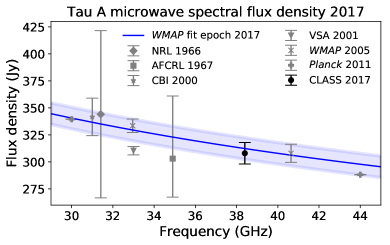
Figure 5: Tau A flux density measurements found in Table 2 and referenced to epoch 2017. The solid line is the WMAP $22\text{\,}\mathrm{GHz}$ to $93\text{\,}\mathrm{GHz}$ Tau A flux density vs frequency model: log S(Jy) = $2.502-0.350$ log($\nu$/$40\text{\,}\mathrm{GHz}$) (Weiland et al., 2011), referenced to epoch 2017. The shaded region is the 1$\sigma$ contour of the model’s flux prediction including spectral and time evolution uncertainty. The CLASS intensity map calibrated through the Moon yields a Tau A flux density of $308\pm 11\text{\,}\mathrm{J}\mathrm{y}$ at $\nu_{e}=$38.4\pm 0.2\text{\,}\mathrm{GHz}$$. The $796\text{\,}\mathrm{\SIUnitSymbolMicro sr}$ CLASS beam solid angle dilutes Tau A to an antenna temperature of $8.56\pm 0.27\text{\,}\mathrm{mK}$.

5 Conclusion

In this paper, we have established the basic on-sky performance of the CLASS telescopes. The stability and time constants of the Q-band TES bolometers are within specification. The array average $1.6\text{\,}\mathrm{pW}$ optical loading, $19\text{\,}\mathrm{a}\mathrm{W}\sqrt{\mathrm{s}}$ NEP, and $27\text{\,}\mathrm{K}$ system noise temperature satisfy the design targets. A $13.1\pm 0.3\text{\,}\mathrm{K}\text{\,}{\mathrm{pW}}^{-1}$ calibration factor that converts from optical power measured at the bolometer to Rayleigh-Jeans temperature on the sky is obtained from fitting hundreds of Moon observations to a Moon brightness temperature model that follows the Moon’s orbit and phase. This calibration factor translates to a telescope optical efficiency of $0.48\pm 0.02$ and is used to construct a Tau A intensity map from the nominal CMB scans. We report a Tau A flux density of $308\pm 11\text{\,}\mathrm{J}\mathrm{y}$ at $38.4\pm 0.2\text{\,}\mathrm{GHz}$, consistent with the WMAP Tau A time-dependent spectral flux density model. The 1$\sigma$ error of the CLASS measurement includes the uncertainty in the bandpass center frequency, the calibration to antenna temperature, and the Tau A peak amplitude.

Between June 2016 and March 2018, CLASS carried out the largest ground-based Q-band CMB sky survey to date, covering $75\%$ of the sky. Comparable large-scale ground-based surveys at low-frequencies include Génova-Santos et al. (2017) and Jones et al. (2018). During this initial CLASS observing campaign, 64 Q-band bolometers were optically sensitive, with a median per detector NET of $258\text{\,}\mathrm{\SIUnitSymbolMicro}\mathrm{K}_{\mathrm{cmb}}\sqrt{\mathrm{s}}$, which implies a median instantaneous array sensitivity of $32\text{\,}\mathrm{\SIUnitSymbolMicro}\mathrm{K}_{\mathrm{cmb}}\sqrt{\mathrm{s}}$. For comparison, the combined polarization sensitivity of the four WMAP $41\text{\,}\mathrm{GHz}$ radiometers was $469\text{\,}\mathrm{\SIUnitSymbolMicro}\mathrm{K}_{\mathrm{cmb}}\sqrt{\mathrm{s}}$ (Jarosik et al., 2003), and the combined sensitivity of the six Planck $44\text{\,}\mathrm{GHz}$ radiometers was $174\text{\,}\mathrm{\SIUnitSymbolMicro}\mathrm{K}_{\mathrm{cmb}}\sqrt{\mathrm{s}}$ (Planck Collaboration et al., 2016a).

This is the first of a series of papers to be published on the initial two years of CLASS $40\text{\,}\mathrm{GHz}$ observations. Additional articles will present the CLASS beam and window function, CLASS polarization modulation and stability, CMB survey maps, and science results derived therefrom. Beyond the first two years, the $40\text{\,}\mathrm{GHz}$ telescope continues to acquire data together with a $90\text{\,}\mathrm{GHz}$ telescope that was installed in 2018. An additional telescope at $90\text{\,}\mathrm{GHz}$ and a 150/220 dichroic telescope will be installed in the near future. The nominal survey ends in late 2021 with plans for extensions thereon.

Acknowledgements

We acknowledge the National Science Foundation Division of Astronomical Sciences for their support of CLASS under Grant Numbers 0959349, 1429236, 1636634, and 1654494. The CLASS project employs detector technology developed under several previous and ongoing NASA grants. Detector development work at JHU was funded by NASA grant number NNX14AB76A. K. Harrington is supported by NASA Space Technology Research Fellowship grant number NX14AM49H. Bastián Pradenas is supported by the Fondecyt Regular Project No. 1171811 (CONICYT) and CONICYT-PFCHA Magister Nacional Scholarship 2016-22161360. We thank the anonymous reviewer for his or her careful reading of our manuscript and many insightful comments and suggestions. We thank Philip Mauskopf for useful discussions of bolometer noise. We acknowledge important contributions from Keisuke Osumi, Mark Halpern, Mandana Amiri, Gary Rhodes, Janet Weiland, Keisuke Osumi, Mario Aguilar, Yunyang Li, Isu Ravi, Tiffany Wei, Connor Henley, Max Abitbol, Lindsay Lowry, and Fletcher Boone. We thank William Deysher, Maria Jose Amaral, and Chantal Boisvert for administrative support. We acknowledge productive collaboration with Dean Carpenter and the JHU Physical Sciences Machine Shop team. Part of this research project was conducted using computational resources at the Maryland Advanced Research Computing Center (MARCC). Some of the results in this paper have been derived using the HEALPix package (Górski et al., 2005). We further acknowledge the very generous support of Jim and Heather Murren (JHU A&S ’88), Matthew Polk (JHU A&S Physics BS ’71), David Nicholson, and Michael Bloomberg (JHU Engineering ’64). CLASS is located in the Parque Astronómico Atacama in northern Chile under the auspices of the Comisión Nacional de Investigación Científica y Tecnológica de Chile (CONICYT). R.D. and P.F. thank CONICYT for grants Anillo ACT-1417, QUIMAL 160009, and BASAL AFB-170002.

References

- Ade et al. (2009) Ade, P. A. R., Chuss, D. T., Hanany, S., et al. 2009, Journal of Physics: Conference Series, 155, 012006
- Albrecht & Steinhardt (1982) Albrecht, A., & Steinhardt, P. J. 1982, Physical Review Letters, 48, 1220
- Allison et al. (2015) Allison, R., Caucal, P., Calabrese, E., Dunkley, J., & Louis, T. 2015, Phys. Rev. D, 92, 123535
- Appel et al. (2014) Appel, J. W., Ali, A., Amiri, M., et al. 2014, in Proc. SPIE, Vol. 9153, Millimeter, Submillimeter, and Far-Infrared Detectors and Instrumentation for Astronomy VII, 91531J
- Battistelli et al. (2008) Battistelli, E. S., Amiri, M., Burger, B., et al. 2008, Journal of Low Temperature Physics, 151, 908
- Bennett et al. (2013) Bennett, C. L., Larson, D., Weiland, J. L., et al. 2013, ApJS, 208, 20
- BICEP2 Collaboration et al. (2016) BICEP2 Collaboration, Keck Array Collaboration, Ade, P. A. R., et al. 2016, Physical Review Letters, 116, 031302
- BICEP2 Collaboration et al. (2018) —. 2018, Physical Review Letters, 121, 221301
- Bustos et al. (2014) Bustos, R., Rubio, M., Otárola, A., & Nagar, N. 2014, Publications of the Astronomical Society of the Pacific, 126, 1126
- Cartwright (2003) Cartwright, J. K. 2003, PhD thesis, California Institute of Technology
- Cartwright et al. (2005) Cartwright, J. K., Pearson, T. J., Readhead, A. C. S., et al. 2005, ApJ, 623, 11
- Chuss et al. (2012a) Chuss, D. T., Wollack, E. J., Henry, R., et al. 2012a, Appl. Opt., 51, 197
- Chuss et al. (2012b) Chuss, D. T., Bennett, C. L., Costen, N., et al. 2012b, Journal of Low Temperature Physics, 167, 923
- Chuss et al. (2014) Chuss, D. T., Ali, A., Appel, J. W., et al. 2014, in American Astronomical Society Meeting Abstracts #223, Vol. 223, 439.03
- Dahal et al. (2018) Dahal, S., Ali, A., Appel, J. W., et al. 2018, in Society of Photo-Optical Instrumentation Engineers (SPIE) Conference Series, Vol. 10708, Society of Photo-Optical Instrumentation Engineers (SPIE) Conference Series, 107081Y
- Denis et al. (2009) Denis, K. L., Cao, N. T., Chuss, D. T., et al. 2009, in American Institute of Physics Conference Series, ed. B. Young, B. Cabrera, & A. Miller, Vol. 1185, 371–374
- Denis et al. (2016) Denis, K. L., Ali, A., Appel, J., et al. 2016, Journal of Low Temperature Physics, 184, 668
- Doriese et al. (2016) Doriese, W. B., Morgan, K. M., Bennett, D. A., et al. 2016, Journal of Low Temperature Physics, 184, 389
- Eimer et al. (2012) Eimer, J. R., Bennett, C. L., Chuss, D. T., et al. 2012, in Society of Photo-Optical Instrumentation Engineers (SPIE) Conference Series, Vol. 8452, Society of Photo-Optical Instrumentation Engineers (SPIE) Conference Series
- Essinger-Hileman et al. (2014) Essinger-Hileman, T., Ali, A., Amiri, M., et al. 2014, in SPIE, Vol. 915354, Millimeter, Submillimeter, and Far-Infrared Detectors and Instrumentation for Astronomy VII
- Fixsen (2009) Fixsen, D. J. 2009, ApJ, 707, 916
- Génova-Santos et al. (2017) Génova-Santos, R., Rubiño-Martín, J. A., Peláez-Santos, A., et al. 2017, MNRAS, 464, 4107
- Górski et al. (2005) Górski, K. M., Hivon, E., Banday, A. J., et al. 2005, ApJ, 622, 759
- Green (2009) Green, D. A. 2009, Bulletin of the Astronomical Society of India, 37, 45
- Guth (1981) Guth, A. H. 1981, Phys. Rev. D, 23, 347
- Hafez et al. (2008) Hafez, Y. A., Davies, R. D., Davis, R. J., et al. 2008, MNRAS, 388, 1775
- Harrington et al. (2016) Harrington, K., Marriage, T., Ali, A., et al. 2016, in Proc. SPIE, Vol. 9914, Millimeter, Submillimeter, and Far-Infrared Detectors and Instrumentation for Astronomy VIII, 99141K
- Harrington et al. (2018) Harrington, K., Eimer, J., Chuss, D. T., et al. 2018, in Society of Photo-Optical Instrumentation Engineers (SPIE) Conference Series, Vol. 10708, Society of Photo-Optical Instrumentation Engineers (SPIE) Conference Series, 107082M
- Henning et al. (2018) Henning, J. W., Sayre, J. T., Reichardt, C. L., et al. 2018, ApJ, 852, 97
- Hinshaw et al. (2013) Hinshaw, G., Larson, D., Komatsu, E., et al. 2013, ApJS, 208, 19
- Hobbs et al. (1968) Hobbs, R. W., Corbett, H. H., & Santini, N. J. 1968, ApJ, 152, 43
- Hu et al. (2017) Hu, G.-P., Chan, K. L., Zheng, Y.-C., Tsang, K. T., & Xu, A.-A. 2017, Icarus, 294, 72
- Irwin & Hilton (2005) Irwin, K., & Hilton, G. 2005, in Topics in Applied Physics, Vol. 99, Cryogenic Particle Detection, ed. C. Enss (Springer Berlin / Heidelberg), 81–97
- Iuliano et al. (2018) Iuliano, J., Eimer, J., Parker, L., et al. 2018, in Society of Photo-Optical Instrumentation Engineers (SPIE) Conference Series, Vol. 10708, Society of Photo-Optical Instrumentation Engineers (SPIE) Conference Series, 1070828
- Jarosik et al. (2003) Jarosik, N., Barnes, C., Bennett, C. L., et al. 2003, ApJS, 148, 29
- Jarosik et al. (2011) Jarosik, N., Bennett, C. L., Dunkley, J., et al. 2011, ApJS, 192, 14
- Jones et al. (2018) Jones, M. E., Taylor, A. C., Aich, M., et al. 2018, MNRAS, 480, 3224
- Kalaghan & Wulfsberg (1967) Kalaghan, P. M., & Wulfsberg, K. N. 1967, AJ, 72, 1051
- Kamionkowski et al. (1997) Kamionkowski, M., Kosowsky, A., & Stebbins, A. 1997, Phys. Rev. D, 55, 7368
- Kovac et al. (2002) Kovac, J. M., Leitch, E. M., Pryke, C., et al. 2002, Nature, 420, 772
- Krotikov & Pelyushenko (1987) Krotikov, V. D., & Pelyushenko, S. A. 1987, Soviet Ast., 31, 216
- Krotikov & Troitskiĭ (1964) Krotikov, V. D., & Troitskiĭ, V. S. 1964, Soviet Physics Uspekhi, 6, 841
- Kusaka et al. (2014) Kusaka, A., Essinger-Hileman, T., Appel, J. W., et al. 2014, Review of Scientific Instruments, 85, 024501
- Kusaka et al. (2018) Kusaka, A., Appel, J., Essinger-Hileman, T., et al. 2018, J. Cosmology Astropart. Phys, 9, 005
- Linde (1982) Linde, A. D. 1982, Physics Letters B, 108, 389
- Linsky (1966) Linsky, J. L. 1966, Icarus, 5, 606
- Linsky (1973) —. 1973, ApJS, 25, 163
- Louis et al. (2017) Louis, T., Grace, E., Hasselfield, M., et al. 2017, J. Cosmology Astropart. Phys, 6, 031
- Martin & Puplett (1970) Martin, D. H., & Puplett, E. 1970, Infrared Physics, 10, 105
- Mather (1982) Mather, J. C. 1982, Appl. Opt., 21, 1125
- Miller et al. (2016) Miller, N. J., Chuss, D. T., Marriage, T. A., et al. 2016, ApJ, 818, 151
- Page et al. (2003a) Page, L., Barnes, C., Hinshaw, G., et al. 2003a, ApJS, 148, 39
- Page et al. (2003b) Page, L., Jackson, C., Barnes, C., et al. 2003b, ApJ, 585, 566
- Petroff et al. (2019) Petroff, M., Appel, J., Rostem, K., et al. 2019, Review of Scientific Instruments, 90, 024701
- Planck Collaboration et al. (2015) Planck Collaboration, Ade, P. A. R., Aghanim, N., et al. 2015, A&A, 576, A104
- Planck Collaboration et al. (2016a) —. 2016a, A&A, 594, A2
- Planck Collaboration et al. (2016b) —. 2016b, A&A, 594, A20
- Planck Collaboration et al. (2016c) —. 2016c, A&A, 594, A26
- Planck Collaboration et al. (2018a) Planck Collaboration, Akrami, Y., Ashdown, M., et al. 2018a, ArXiv e-prints, arXiv:1807.06208
- Planck Collaboration et al. (2018b) Planck Collaboration, Aghanim, N., Akrami, Y., et al. 2018b, ArXiv e-prints, arXiv:1807.06209
- Planck Collaboration et al. (2018c) Planck Collaboration, Akrami, Y., Arroja, F., et al. 2018c, ArXiv e-prints, arXiv:1807.06211
- Planck Collaboration et al. (2018d) Planck Collaboration, Akrami, Y., Ashdown, M., et al. 2018d, ArXiv e-prints, arXiv:1801.04945
- Planck Collaboration Int. L (2017) Planck Collaboration Int. L. 2017, A&A, 599, A51
- Polarbear Collaboration et al. (2014) Polarbear Collaboration, Ade, P. A. R., Akiba, Y., et al. 2014, ApJ, 794, 171
- Rees (1968) Rees, M. J. 1968, ApJ, 153, L1
- Richards (1994) Richards, P. L. 1994, Journal of Applied Physics, 76, 1
- Ritacco et al. (2018) Ritacco, A., Macías-Pérez, J. F., Ponthieu, N., et al. 2018, A&A, 616, A35
- Rostem et al. (2012) Rostem, K., Bennett, C. L., Chuss, D. T., et al. 2012, in Society of Photo-Optical Instrumentation Engineers (SPIE) Conference Series, Vol. 8452, Society of Photo-Optical Instrumentation Engineers (SPIE) Conference Series
- Rostem et al. (2014a) Rostem, K., Chuss, D. T., Colazo, F. A., et al. 2014a, Journal of Applied Physics, 115, 124508
- Rostem et al. (2014b) Rostem, K., Ali, A., Appel, J. W., et al. 2014b, in Proc. SPIE, Vol. 9153, Millimeter, Submillimeter, and Far-Infrared Detectors and Instrumentation for Astronomy VII, 91530B
- Sato (1981) Sato, K. 1981, MNRAS, 195, 467
- Starobinsky (1982) Starobinsky, A. A. 1982, Physics Letters B, 117, 175
- Troitskii (1967) Troitskii, V. S. 1967, Radiophysics and Quantum Electronics, 10, 709
- Troitskii & Tikhonova (1970) Troitskii, V. S., & Tikhonova, T. V. 1970, Radiophysics and Quantum Electronics, 13, 981
- Troitsky et al. (1968) Troitsky, V. S., Burov, A. B., & Alyoshina, T. N. 1968, Icarus, 8, 423
- Tsang et al. (2016) Tsang, K., Hu, G.-P., & Zheng, Y.-C. 2016, in AAS/Division for Planetary Sciences Meeting Abstracts, Vol. 48, AAS/Division for Planetary Sciences Meeting Abstracts #48, 223.06
- van Vliet (1967) van Vliet, K. M. 1967, Appl. Opt., 6, 1145
- Watts et al. (2015) Watts, D. J., Larson, D., Marriage, T. A., et al. 2015, ApJ, 814, 103
- Watts et al. (2018) Watts, D. J., Wang, B., Ali, A., et al. 2018, ApJ, 863, 121
- Weiland et al. (2011) Weiland, J. L., Odegard, N., Hill, R. S., et al. 2011, ApJS, 192, 19
- Zaldarriaga & Seljak (1997) Zaldarriaga, M., & Seljak, U. 1997, Phys. Rev. D, 55, 1830
- Zeng (2012) Zeng, L. 2012, PhD thesis, The Johns Hopkins University
- Zheng et al. (2012) Zheng, Y. C., Tsang, K. T., Chan, K. L., et al. 2012, Icarus, 219, 194
- Zmuidzinas (2003) Zmuidzinas, J. 2003, Appl. Opt., 42, 4989