Abstract

The leptonic radiative decay $B\to\gamma l\nu$ is of great importance in the determination of $B$ meson wave functions, and evaluating the form factors $F_{V,A}$ are the essential problem on the study of this channel. We computed next-to-leading power corrections to the form factors within the framework of PQCD approach, including the power suppressed hard kernel, the contribution from a complete set of three-particle $B$ meson wave functions up to twist-4 and two-particle off light-cone wave functions, the $1/m_{b}$ corrections in heavy quark effective theory, and the contribution from hadronic structure of photon. In spite of large theoretical uncertainties, the overall power suppressed contributions decreases about $50\%$ of the leading power result. The $\lambda_{B}$ dependence of the integrated branching ratio is reduced after including the subleading power contributions, thus the power corrections lead to more ambiguity in the determination of $\lambda_{B}$ from $B\to\gamma l\nu$ decay.

1 Introduction

$k_{T}$ factorization theorem is an appropriate theoretical framework for exclusive $B$ meson decays. By retaining parton transverse momenta $k_{T}$, the end-point singularities which break collinear factorization is regularized. The PQCD approach[1, 2] based on the $k_{T}$ factorization framework has been applied to various exclusive processes, especially semi-leptonic and non-leptonic $B$-meson decays, and other decay modes[3]. The resultant predictions are in agreement with most of the experimental data, and the most applaudable result is the CP violation in many non-leptonic $B$-meson decay channels. The LHC-b and forthcoming Super-B factory experiments will accumulate more and more accurate data, which require more precise theoretical predictions. To achieve this target, both QCD radiative corrections and power corrections need to be considered. In PQCD approach, QCD radiative corrections are extensively studied in many processes, such as the pion transition form factor[4, 5], the pion electro-magnetic form factors[6, 7, 8], the $B\to\pi$ form factors[9, 10], et al., while the exploration on power corrections are very few. The motivation of this paper is to investigate the power corrections in the leptonic radiative decay mode $B\to\gamma l\nu$.

Most of the theoretical frameworks to study $B$ meson decays are based on heavy quark expansion, and power corrections are important for finite $b$ quark mass. While in the collinear factorization, the power suppressed contributions are in general non-factorizable due to end-point singularity, so they are often fitted by experimental data or estimated using non-perturbative methods. $1/m_{b}$ power corrections to $B\to\gamma\ell\nu$ were considered at tree level [11] where a symmetry-conserving form factor $\xi(E_{\gamma})$ was introduced to parameterize the non-local power correction. An approach based on dispersion relations and quark-hadron duality was employed to study the power suppressed contributions in $B\to\gamma\ell\nu$ [12], where the “soft” two-particle correction to the $B\to\gamma$ form factors was computed at leading order. The one-loop corrections to this kind of subleading power contribution has been computed in [13], in addition the contribution from three-particle light-cone distribution amplitudes(LCDAs) was also considered at tree level. In a recent paper[14], using dispersion approach, the soft contribution of power-suppressed higher-twist corrections to the form factors that are due to higher Fock states of $B$-meson and to the transverse momentum (virtuality) of the light quark in the valence state was calculated, the results are found to be much smaller than that of twist-2 contribution. Based on the power counting in the soft-collinear effective theory(SCET [15, 16]), the hadronic structure of photon can contribute at next-to-leading power, which was studied in [17, 18]. The soft contribution and the contribution from the hadronic structure of photon are probably closely related, and it is interesting to uncover their relationship.

In the PQCD approach, tree-level power corrections have been firstly studied in [19], and a more careful investigation of power corrections was performed in Ref.[20], in which three-particle $B$-meson wave functions, next-to-leading power(NLP) hard kernels, and long-distance vector meson dominance contribution are considered. In [20] the contribution from an incomplete set of three-particle $B$ meson LCDAs was estimated by power counting, but the detailed calculation is still absent. The long distance contribution is found to be cancelled by the radiative corrections, which makes the power correction very small. As a rough estimate, this conclusion needs to be checked by a more careful calculation. Our aim in this article is to make the following improvements: (1) The contribution from a complete set of higher twist $B$ meson wave functions, up to twist-4, will be investigated. The higher twist wave functions include both two-particle and three-particle Fock states, which are related by the equation of motion. (2) The contribution from the hadronic structure of photon will be calculated within PQCD framework. As the endpoint singularity appears in the collinear factorization is regularized by including the transverse momentum, this kind of contribution can be studied using factorization approach. (3) The $1/m_{b}$ corrections to the heavy-to-light current in HQET will be considered. Although the NLP contributions considered here are still far from a systematical study, but they can shed light on the correction arises from the power corrections, which makes great sense in the determination of the parameter $\lambda_{B}$.

This paper is organized as follows: In the next section we will present the analytic calculation of the decay amplitude of $B\to\gamma l\nu$, including both leading power(LP) and NLP contributions. The numerical analysis is given in the third section. Concluding discussions are presented in Section 4.

2 The $B\to\gamma l\nu$ decay amplitude at next-to-leading power

The radiative leptonic B-meson decay amplitude is given by

$$A(B\to\gamma\nu l)={G_{F}V_{ub}\over\sqrt{2}}\langle\gamma l\nu_{l}|\bar{l}\gamma^{\nu}(1-\gamma_{5})\nu_{l}\bar{u}\gamma_{\nu}(1-\gamma_{5})b|B\rangle.$$ (1)

At leading order in QED, the above amplitude can be written as

$$A(B\to\gamma\nu l)={G_{F}V_{ub}\over\sqrt{2}}(ig_{em}\epsilon^{*}_{\nu})[T^{\nu\mu}(p,q)\bar{l}\gamma_{\mu}(1-\gamma_{5})\nu+Q_{l}f_{B}\bar{l}\gamma_{\nu}(1-\gamma_{5})\nu],$$ (2)

where the momenta carried by photon, lepton-pair and $B$-meson are $p,q$ and $p+q$ respectively. In the light-cone coordinate, $p_{\mu}={n\cdot p\over 2}\bar{n}_{\mu}=E_{\gamma}\bar{n}_{\mu}$, $q_{\mu}={1\over 2}(n\cdot q\bar{n}_{\mu}+\bar{n}\cdot qn_{\mu})$ and $p_{\mu}+q_{\mu}=m_{B}v_{\mu}$. The hadronic tensor $T_{\nu\mu}$ reads

$$T_{\nu\mu}(p,q)=\int d^{4}ze^{ip\cdot z}\langle 0|{\rm T}[j^{em}_{\nu}(z),\bar{u}(0)\gamma_{\mu}(1-\gamma_{5})b(0)]|B(p+q)\rangle,$$ (3)

with $j^{em}_{\nu}(z)=\sum_{q}Q_{q}\bar{q}(z)\gamma_{\nu}q(z)+Q_{l}\bar{l}(z)\gamma_{\nu}l(z)$. Considering vector and axial vector current conservation, the decomposition of the hadronic matrix element reads

$$T_{\nu\mu}(p,q)=-iv\cdot p\epsilon_{\mu\nu\rho\sigma}n^{\rho}v^{\sigma}F_{V}(n\cdot p)+(g_{\mu\nu}v\cdot p-v_{\nu}p_{\mu})F_{A}(n\cdot p)+g_{\mu\nu}f_{B},$$ (4)

where the last term will cancel the contribution with photon radiated from the lepton. The differential decay rate of $B\to\gamma l\nu$ can be readily computed using the following formula

$${d\Gamma\over dE_{\gamma}}(B\to\gamma l\nu)={\alpha_{em}G_{F}^{2}|V_{ub}|^{2}\over 6\pi^{2}}m_{B}E_{\gamma}^{3}(1-{2E_{\gamma}\over m_{B}})[F_{V}^{2}(n\cdot p)+F_{A}^{2}(n\cdot p)].$$ (5)

This equation indicates that the essential problem in the $B\to\gamma l\nu$ decays is to study the factorization of the form factors $F_{A,V}$. A systematical study on the power corrections for this process needs to analyze power suppressed SCET operators, which is rather complicated and we leave it for a future study. Alternatively, we follow [14] to expand the matrix element using heavy quark effective theory(HQET)

$$T_{\nu\mu} = \sqrt{m_{B}}\int d^{4}ze^{ip\cdot z}\langle 0|{\rm T}[j^{em}_{\nu}(z),\bar{u}\gamma_{\mu}(1-\gamma_{5})h_{v}(0)]|B(v)\rangle$$ (6)

$$+ {\sqrt{m_{B}}\over 2m_{b}}\int d^{4}ze^{ip\cdot z}\langle 0|{\rm T}[j^{em}_{\nu}(z),\bar{u}\gamma_{\mu}(1-\gamma_{5})i\not\!D_{\perp}h_{v}(0)]|B(v)\rangle.$$

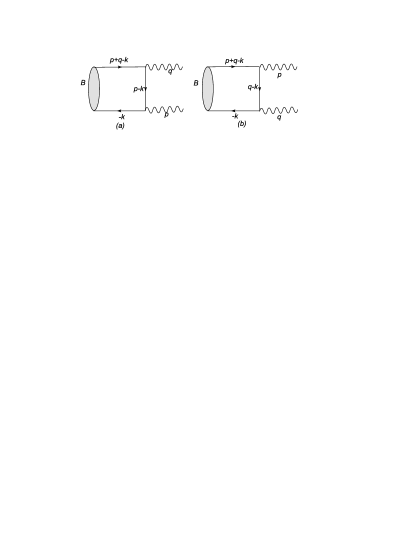
Figure 1: Tree level diagrams with two-particle $B$ meson wave functions.

In the first line, the power corrections arise from the light-cone expansion of quark propagator

$$\langle 0|T\{q(z),\bar{q}(0)\}|0\rangle={i\over 2\pi^{2}}{\not\!z\over z^{4}}-\frac{i}{16\pi^{2}}\frac{1}{z^{2}}\int^{1}_{0}du[\not\!z\sigma_{\alpha\beta}-4iuz_{\alpha}\gamma_{\beta}]G^{\alpha\beta}(uz)+...,$$ (7)

and the twist expansion of $B$-meson wave functions[22, 23, 24, 25, 26, 29]

$$\langle 0|{\bar{q}}(z)W_{z}(n)^{{\dagger}}I_{n;y,0}W_{0}(n)\Gamma h(0)|{\bar{B}}(v)\rangle = -{if_{B}m_{B}\over 4}{\rm Tr}\bigg{\{}{1+/\!\!\!v\over 2}\bigg{[}2\,\Phi_{B}^{+}(t,z^{2})+2z^{2}G^{+}(z^{2})$$ (8)

$$+ {\Phi_{B}^{-}(t,z^{2})+z^{2}G^{-}(z^{2})-\Phi_{B}^{+}(t,z^{2})-z^{2}G^{+}(z^{2})\over t}/\!\!\!z+...\bigg{]}\gamma_{5}\,\Gamma\bigg{\}}.$$

The $B$ meson wave functions describe the distributions of the light parton in both the longitudinal direction denoted by $t=v\cdot z$ and the transverse direction denoted by $z^{2}$. In the above definition $z=(0,z^{-},{\bf z}_{T})$ is the coordinate of the anti-quark field $\bar{q}$, $h$ is the $b$ quark field in the heavy quark effective theory, and $\Gamma$ represents a Dirac matrix. The Wilson line $W_{z}(n)$ is written as

$$W_{z}(n)={P}\exp\left[-ig\int_{0}^{\infty}d\lambda n\cdot A(z+\lambda n)\right].$$ (9)

The vertical link $I_{n;z,0}$ at infinity does not contribute in the covariant gauge [30]. Due to the light-cone divergences associated with the Wilson lines, the light-cone vector should be rotated to satisfy $n^{2}\not=0$. The wave functions $\Phi_{B}^{\pm}(t,z^{2})$ are twist-2, and $G^{\pm}(z^{2})$ are twist-4. In addition, the definition of three-particle LCDAs is as follows

$$\langle 0|\bar{q}_{2\alpha}(z)G_{\mu\nu}(uz)b_{\beta}(0)|\bar{B}_{v}\rangle = \frac{f_{B}m_{B}}{4}\int_{0}^{\infty}d\omega\int_{0}^{\infty}d\xi\int{d^{2}k_{1\perp}\over(2\pi)^{2}}\int{d^{2}k_{2\perp}\over(2\pi)^{2}}e^{-i(k_{1}+uk_{2})\cdot z}$$ (10)

$$\times \bigg{[}(1+/\!\!\!v)\bigg{\{}(v_{\mu}\gamma_{\nu}-v_{\nu}\gamma_{\mu})[\psi_{A}-\psi_{V}]-i\sigma_{\mu\nu}\psi_{V}-(\bar{n}_{\mu}v_{\nu}-\bar{n}_{\nu}v_{\mu})X_{A}$$

$$+ (\bar{n}_{\mu}\gamma_{\nu}-\bar{n}_{\nu}\gamma_{\mu})(W+Y_{A})+i\epsilon_{\mu\nu\rho\sigma}\bar{n}^{\rho}v^{\sigma}\gamma_{5}\tilde{X}-i\epsilon_{\mu\nu\rho\sigma}\bar{n}^{\rho}\gamma^{\sigma}\gamma_{5}\tilde{Y}$$

$$- (\bar{n}_{\mu}v_{\nu}-\bar{n}_{\nu}v_{\mu})\not\!\bar{n}W+(\bar{n}_{\mu}\gamma_{\nu}-\bar{n}_{\nu}\gamma_{\mu})\not\!\bar{n}Z\bigg{\}}\gamma_{5}\bigg{]}_{\beta\alpha}(\omega,\xi,k_{1\perp},k_{2\perp}).$$

The wave functions defined above do not have definite twist, but they are convenient in the calculation for their simple Lorentz structure.

For the second line of Eq.(6), although there already exists a suppressed factor $1/m_{b}$, higher twist $B$ meson wave functions are still required as the power expansion in terms of $1/m_{b}$ is not equivalent to the twist expansion. In the following we will consider the contribution from leading twist and higher twist $B$ meson wave functions respectively in the first line of Eq.(6), and then evaluate the contribution from the second line Eq.(6). Furthermore, we will also investigate the contribution from the hadronic structure of photon at the last subsection.

2.1 Contribution from leading twist $B$ meson wave functions

Firstly we consier LP result of $F_{V,A}$ and NLP corrections from leading twist $B$ meson wave functions. From the definition in Eq.(8), the momentum space projector for $B$-meson twist-2 wave functions can be written by

$$M^{B}_{\alpha\beta}=-\frac{if_{B}m_{B}}{4}\Bigg{[}\frac{1+\not\!v}{2}\Bigg{\{}\phi^{+}_{B}(\omega,k_{\perp})\,\not\!n+\phi^{-}_{B}(\omega,k_{\perp})\,\not\!\bar{n}-\,\int_{0}^{\omega}d\eta\,\left(\phi^{-}_{B}(\eta,k_{\perp})-\phi^{+}_{B}(\eta,k_{\perp})\right)\,\gamma^{\mu}\frac{\partial}{\partial k_{\perp\mu}}\Bigg{\}}\,\gamma_{5}\Bigg{]}_{\alpha\beta}.$$ (11)

The leading power contribution is from Fig.(1a), in which the light quark propagator can be decomposed as

$${i(\not\!p-\not\!k)\over(p-k)^{2}}=-i{E_{\gamma}\not\!\bar{n}\over 2E_{\gamma}\omega+k_{\perp}^{2}}+i{\omega\not\!v\over 2E_{\gamma}\omega+k_{\perp}^{2}}-i{\not\!k_{\perp}\over 2E_{\gamma}\omega+k_{\perp}^{2}},$$ (12)

where the first term is at leading power, and the other two terms are suppressed by $\lambda={\omega\over E_{\gamma}}$. Taking only the leading power contribution into account, the form factors $F_{V,A}$ can be written by

$$F_{A}^{LP}(E_{\gamma})=F_{V}^{LP}(E_{\gamma})={2\over 3}f_{B}m_{B}\int_{0}^{1}d\omega\int{d^{2}k_{\perp}\over(2\pi)^{2}}{\phi^{+}_{B}(\omega,k_{\perp})\over 2\omega E_{\gamma}+k_{\perp}^{2}}.$$ (13)

According to [20], the mass dependence of the hadron state arises if the power suppressed operators $O_{1,2}$ are included

$$\langle 0|{\bar{u}}_{\rho}(z)h_{\delta}(0)|\bar{B}(Mv)\rangle_{QCD}=\sum_{i=1,2}\langle 0|i\int d^{4}yT[{\bar{u}}_{\rho}(z)h_{\delta}(0)O_{i}(y)]|\bar{B}(v)\rangle\;.$$ (14)

where

$$O_{1}=\frac{1}{m_{b}}\bar{h}(iD)^{2}h\;,\;\;\;O_{2}=\frac{g}{2m_{b}}\bar{h}\sigma^{\mu\nu}G_{\mu\nu}h\;.$$ (15)

After considering the mass dependence of the hadronic state the momentum fraction of the soft quark inside the $B$ meson can be defined by $x=\omega/m_{B}$, and Eq.(13) turns to

$$F_{A}^{LP}(E_{\gamma})=F_{V}^{LP}(E_{\gamma})={2\over 3}f_{B}m_{B}\int_{0}^{1}dx\int{d^{2}k_{\perp}\over(2\pi)^{2}}{\phi^{+}_{B}(x,k_{\perp})\over 2xm_{B}E_{\gamma}+k_{\perp}^{2}}.$$ (16)

The QCD correction to the $B$ meson wave functions and the leading-order (LO) hard kernel produces both the single and double logarithms $\ln^{2}{k_{\perp}\over E_{\gamma}}$, $\ln{k_{\perp}\over E_{\gamma}}$, $\ln^{2}x$ and $\ln x$ respectively, which become large as $k_{\perp}\ll E_{\gamma},x\ll 1$. These large logarithms need to be resummed, among them $k_{T}$ resummation leads to Sudakov form factor, and threshold resummation(resumming $\ln^{2}x$ and $\ln x$) leads to jet function. The $k_{T}$ and threshold resummation improves the convergence of the perturbation series, and the resummation improved factorization formula can be rewritten by

$$F_{A}^{LP}(E_{\gamma})=F_{V}^{LP}(E_{\gamma})={2\over 3}f_{B}m_{B}\int_{0}^{1}dx\int_{0}^{\infty}bdbK_{0}(\sqrt{2xE_{\gamma}m_{B}}b)S_{t}(x)e^{-s_{B}(t)}\phi^{+}_{B}(x,b),$$ (17)

where $s_{B}(t)$ is the Sudakov form factor and $S_{t}(x)$ is the jet function from the threshold resummation[1, 2]. The threshold factor from the resummation of $\ln^{2}x$ has been parameterized as

$$S_{t}(x,Q) = {2^{1+c(Q^{2})}\,\Gamma({3\over 2}+c(Q^{2}))\over\sqrt{\pi}\,\Gamma(1+c(Q^{2}))}\,\left[x(1-x)\right]^{c(Q^{2})}\,.$$ (18)

Both the hard kernel and the wave function have been transformed into the impact parameter space($b$ space) because it is more convenient to perform sudakov resummation in $b$ space. In the above equation the resummation of rapidity logarithms $\ln{(n\cdot p)^{2}\over n^{2}}$, which will cause scheme dependence, is neglected. In [31] the joint resummation with respect to all the large logarithms is performed, and this effect will be considered in the future study.

The power suppressed amplitude includes the latter two terms in Eq.(12) and the contribution from Fig(1b). We note that the last term in Eq.(12), which is related to the transverse derivative in the $B$-meson wave function(the last term in Eq.(11)), vanishes in 4-dimension due to the Lorentz structure $\gamma_{\perp\mu}\not\!\epsilon^{*}_{\perp}\gamma_{\perp}^{\mu}$. The second term in Eq.(12) results in

$$F_{A}^{NP1a}(E_{\gamma}) = -{1\over 3E_{\gamma}}f_{B}m_{B}^{2}\int_{0}^{1}dxx\int_{0}^{\infty}bdbS_{t}(x)e^{-s_{B}(t)}K_{0}(\sqrt{2xE_{\gamma}m_{B}}b)[\phi^{-}_{B}(x,b)+\phi^{+}_{B}(x,b)]$$

$$F_{V}^{NP1a}(E_{\gamma}) = {1\over 3E_{\gamma}}f_{B}m_{B}^{2}\int_{0}^{1}dxx\int_{0}^{\infty}bdbS_{t}(x)e^{-s_{B}(t)}K_{0}(\sqrt{2xE_{\gamma}m_{B}}b)[\phi^{-}_{B}(x,b)-\phi^{+}_{B}(x,b)].$$ (19)

The internal line in Fig(1b) is a heavy quark propagator, due to the basic idea of effective theory, it must be integrated out and leads to local contribution. In the diagrammatic approach, the propagator is proportional to $1\over 2m_{b}E_{\gamma}+k_{\perp}^{2}$, where $k_{\perp}^{2}$ in the denominator is obviously suppressed, and this term is identical to the collinear factorization result after $k_{\perp}$ is dropped

$$F_{A}^{NLP1b}(E_{\gamma})=-F_{V}^{NLP1b}(E_{\gamma})={f_{B}m_{B}\over 6m_{b}E_{\gamma}}$$ (20)

Adding up the leading twist NLP contribution, we obtain

$$F_{A,V}^{NLP1}(E_{\gamma})=F_{A,V}^{NLP1a}(E_{\gamma})+F_{A,V}^{NLP1b}(E_{\gamma}).$$ (21)

2.2 Contribution from higher twist $B$ meson wave functions

Up to twist-4, the higher twist $B$ meson wave functions include two-particle Fock state, i.e. $G^{\pm}(t,z^{2})$, and three-particle Fock state defined in Eq.(10). According to twist expansion, the three-particle wave functions include one twist-3, $\phi_{3}=\psi_{A}-\psi_{V}$, and three twist-4, $\phi_{4}=\psi_{A}+\psi_{V},\,\psi_{4}=\psi_{A}+X_{A},\,\tilde{\psi}_{4}=\psi_{V}-\tilde{X}_{A}$, in which only two wave functions are independent. We assume that all the wave functions have the factorized form, i.e., $G^{\pm}(t,z^{2})=G^{\pm}_{B}(t)\tilde{\Sigma}(z^{2})$, where $G^{\pm}_{B}(t)$ are $B$-meson LCDAs. The two-particle and three-particle LCDAs are related by the following equation of motion

$$2t^{2}G^{+}_{B}(t)=-\frac{1}{2}\Phi^{-}_{B}(t)-\bigg{(}t\frac{d}{dt}-\frac{1}{2}+it\bar{\Lambda}\bigg{)}\Phi^{+}_{B}(t)-t^{2}\int^{1}_{0}du\bar{u}\Psi_{4}(t,ut),$$ (22)

and it is convenient to define

$$2t^{2}\hat{G}^{+}_{B}(t)=-\frac{1}{2}\Phi^{-}_{B}(t)-\bigg{(}t\frac{d}{dt}-\frac{1}{2}+it\bar{\Lambda}\bigg{)}\Phi^{+}_{B}(t).$$ (23)

The contribution from three-particle Fock state is plotted in Fig.(2). Inserting Eq.(10) and Eq.(7) into the correlation function $T_{\nu\mu}$, one can obtain the factorization formulae of contributions from three-particle $B$-meson wave functions. Combining the three-particle contribution with the contribution from $G^{\pm}(t,z^{2})$, we have

$$F_{A}^{NLP2a}(E_{\gamma})=F_{V}^{NLP2a}(E_{\gamma}) = -{4\over 3}f_{B}m_{B}\int_{0}^{\infty}{d\omega\over\sqrt{2E_{\gamma}\omega}}\int^{\infty}_{0}b^{2}db\hat{g}_{B}^{+}(\omega,b)K_{1}(\sqrt{2E_{\gamma}\omega}b),$$ (24)

$$F_{A}^{NLP2b}(E_{\gamma})=F_{V}^{NLP2b}(E_{\gamma}) = {1\over 3\sqrt{2E_{\gamma}}}f_{B}m_{B}\int_{0}^{\infty}d\omega\int_{0}^{\infty}d\xi\int_{0}^{1}{du\over\sqrt{\omega+u\xi}}\int_{0}^{\infty}b^{2}db$$ (25)

$$\times K_{1}(\sqrt{2E_{\gamma}(\omega+u\xi)}b)\,\left[\psi_{4}(\omega,\xi,b)-\tilde{\psi}_{4}(\omega,\xi,b)\right],$$

where $\hat{G}^{+}({t,b})=\int_{0}^{\infty}d\omega e^{-i\omega t}\hat{g}^{+}({\omega},b)$. The total contribution from high twist wave functions is written by

$$F_{A,V}^{NLP2}(E_{\gamma})=F_{A,V}^{NLP2a}(E_{\gamma})+F_{A,V}^{NLP2b}(E_{\gamma}).$$ (26)

Figure 2: Diagrams of the contribution from three-particle $B$ meson wave functions

2.3 Power suppressed contribution in HQET

To evaluate the $1/m_{b}$ correction in Eq.(6), one should take advantage of the formula

$$\bar{q}(z)\Gamma D_{\rho}h_{v}(0)=\partial_{\rho}[\bar{q}(z)\Gamma h_{v}(0)]+i\int_{0}^{1}du\bar{u}\bar{q}(z)z^{\lambda}G_{\lambda\rho}(zu)\Gamma h_{v}(0)+[{\partial\over\partial z^{\rho}}\bar{q}(z)]\Gamma h_{v}(0).$$ (27)

For the first term in the above equation, using the following relation

$$\langle 0|\partial_{\rho}[\bar{q}(z)\Gamma h_{v}(0)]|B(v)\rangle={\partial\over\partial y^{\rho}}e^{-i\bar{\Lambda}v\cdot y}\langle 0|[\bar{q}(z)\Gamma h_{v}(0)]|B(v)\rangle=-i\bar{\Lambda}v_{\rho}\langle 0|[\bar{q}(z)\Gamma h_{v}(0)]|B(v)\rangle,$$ (28)

one can obtain

$$F_{A}^{NLP3a}(E_{\gamma})=F_{V}^{NLP3a}(E_{\gamma})={\bar{\Lambda}\over 3m_{b}}f_{B}m_{B}\int_{0}^{1}dx\int_{0}^{\infty}bdbK_{0}(\sqrt{2xE_{\gamma}m_{B}}b)S_{t}(x)e^{-s_{B}(t)}\phi^{+}_{B}(x,b).$$ (29)

The matrix element of the second term is related to the twist-3 three-particle wave function, following the same method with the above subsection, we have

$$F_{A}^{NLP3b}(E_{\gamma})=F_{V}^{NLP3b}(E_{\gamma}) = {\sqrt{2E_{\gamma}}\over 3m_{b}}f_{B}m_{B}\int_{0}^{\infty}d\omega\int_{0}^{\infty}d\xi\int_{0}^{1}{du\over\sqrt{\omega+u\xi}}\int_{0}^{\infty}b^{2}db$$ (30)

$$\times K_{1}(\sqrt{2E_{\gamma}(\omega+u\xi)}b)\phi_{3}(\omega,\xi,b).$$

The last term can be evaluated with integration by part, and the result reads

$$F_{A}^{NLP3c}(E_{\gamma})=F_{V}^{NLP3c}(E_{\gamma}) = {f_{B}m_{B}\over 3m_{b}}\int_{0}^{1}dx\int_{0}^{\infty}bdbK_{0}(\sqrt{2xE_{\gamma}m_{B}}b)\Psi_{B}(x,b)$$ (31)

$$- {2f_{B}m_{B}E_{\gamma}\over 3m_{b}}\int_{0}^{1}xdx\int_{0}^{\infty}bdbK_{0}(\sqrt{2xE_{\gamma}m_{B}}b)\phi^{+}_{B}(x,b),$$

with $\Psi_{B}(\omega,b)=\int_{0}^{\omega}d\eta[\phi^{-}(\eta,b)-\phi^{+}(\eta,b)]$. Adding up all the above results we have

$$F_{A,V}^{NLP3}(E_{\gamma})=F_{A,V}^{NLP3a}(E_{\gamma})+F_{A,V}^{NLP3b}(E_{\gamma})+F_{A,V}^{NLP3c}(E_{\gamma}).$$ (32)

2.4 Contribution from hadronic structure of photon

To investigate the contribution of the hadronic structure of photon, it is essential to introduce the LCDAs of photon, which have been studied up to twist-4 level in [37]. In the present paper we will only consider the contribution of two-particle twist-2 and twist-3 LCDAs, which are defined below

$$\langle\gamma(p,\lambda)|\bar{q}(z)\sigma_{\alpha\beta}q(0)|0\rangle = ig_{em}Q_{q}\langle\bar{q}q\rangle(p_{\beta}\epsilon^{*}_{\alpha}-p_{\alpha}\epsilon^{*}_{\beta})\int_{0}^{1}due^{iup\cdot z}[\chi(\mu)\phi_{\gamma}(u,\mu)]$$

$$\langle\gamma(p,\lambda)|\bar{q}(z)\gamma_{\alpha}q(0)|0\rangle = -g_{em}Q_{q}f_{3\gamma}\epsilon^{*}_{\alpha}\int_{0}^{1}due^{iup\cdot z}\psi^{(v)}_{\gamma}(u,\mu)$$

$$\langle\gamma(p,\lambda)|\bar{q}(z)\gamma_{\alpha}\gamma_{5}q(0)|0\rangle = {1\over 4}g_{em}Q_{q}f_{3\gamma}\epsilon_{\alpha\beta\rho\sigma}p^{\rho}z^{\sigma}\epsilon^{*\beta}\int_{0}^{1}due^{iup\cdot z}\psi^{(a)}_{\gamma}(u,\mu)$$ (33)

where $\phi_{\gamma}(u,\mu)$ is twist-2, and $\psi^{(a,v)}_{\gamma}(u,\mu)$ are twist-3. The normalization constants of these LCDAs depend on the factorization scale, and the evolution behavior is written by

$$\chi(\mu) = \left[{\alpha(\mu)\over\alpha_{s}(\mu_{0})}\right]^{16\over 33-2n_{f}}\chi(\mu_{0}),\;\;\;\langle\bar{q}q\rangle(\mu)=\left[{\alpha(\mu_{0})\over\alpha_{s}(\mu)}\right]^{12\over 33-2n_{f}}\langle\bar{q}q\rangle(\mu_{0}),$$ (34)

$$f_{3\gamma}(\mu)=\left[{\alpha_{s}(\mu)\over\alpha_{s}(\mu_{0})}\right]^{23\over 99-6n_{f}}\,f_{3\gamma}(\mu_{0})\,.\qquad$$ (35)

In the factorization formulae we will neglect the transverse momentum dependence of the wave functions, because the Sudakov effect for light $q\bar{q}$ state is significant, and further suppression is not necessary. The momentum space projector for the two-particle LCDAs is written by(up to two-particle twist-3)

$$M^{\gamma}_{\alpha\beta} = {1\over 4}g_{em}Q_{q}\bigg{\{}-\langle\bar{q}q\rangle(\not\!\epsilon^{*}\not\!p)\chi(\mu)\phi_{\gamma}(u,\mu)-f_{3\gamma}(\not\!\epsilon^{*})\psi^{(v)}_{\gamma}(u,\mu)$$ (36)

$$- {i\over 8}f_{3\gamma}\epsilon_{\mu\nu\rho\sigma}(\gamma^{\mu}\gamma^{5}){\bar{n}}^{\rho}\epsilon^{*\nu}[n^{\sigma}{d\over du}\psi^{(a)}_{\gamma}(u,\mu)-2E_{\gamma}\psi^{(a)}_{\gamma}(u,\mu){\partial\over\partial k_{\perp\sigma}}]\bigg{\}}_{\alpha\beta}.$$

The matrix element of $B\to\gamma$ transition can be calculated through the convolution formula

$${}_{HS}\langle\gamma|\bar{q}\Gamma b|B\rangle={4\pi\alpha_{s}C_{F}\over N_{c}}\int_{0}^{1}dx\int_{0}^{\infty}b_{1}db_{1}\int_{0}^{1}du\int_{0}^{\infty}b_{2}db_{2}M^{B}_{\beta\rho}H^{\Gamma}_{\alpha\beta\rho\sigma}M^{\gamma}_{\sigma\alpha},$$ (37)

after evaluating the Feynman diagrams in Fig(3), the results of the form factors $F_{V,A}$ read

$$F_{A}^{NLP4a}(E_{\gamma}) = -{\pi\alpha_{s}C_{F}f_{B}m_{B}Q_{u}\over E_{\gamma}N_{c}}\int_{0}^{1}dx\int_{0}^{\infty}b_{1}db_{1}\int_{0}^{1}du\int_{0}^{\infty}b_{2}db_{2}h^{a}_{e}(x,u,b_{1},b_{2})$$ (38)

$$\times [2E_{\gamma}m_{B}\langle\bar{q}q\rangle\chi(\mu)\phi_{\gamma}(u,\mu)\phi_{B}^{-}-(2uE_{\gamma}\phi_{B}^{+}+m_{B}(\phi_{B}^{-}+\phi_{B}^{+}))f_{3\gamma}\psi^{(v)}$$

$$+ {1\over 2}(uE_{\gamma}\phi_{B}^{+}+{1\over 2}m_{B}(\phi_{B}^{-}-\phi_{B}^{+}))f_{3\gamma}{d\over du}\psi^{(a)}_{\gamma}(u,\mu)],$$

$$F_{V}^{NLP4a}(E_{\gamma}) = -{\pi\alpha_{s}C_{F}f_{B}m_{B}Q_{u}\over E_{\gamma}N_{c}}\int_{0}^{1}dx\int_{0}^{\infty}b_{1}db_{1}\int_{0}^{1}du\int_{0}^{\infty}b_{2}db_{2}h^{a}_{e}(x,u,b_{1},b_{2})$$ (39)

$$\times [2E_{\gamma}m_{B}\langle\bar{q}q\rangle\chi(\mu)\phi_{\gamma}(u,\mu)\phi_{B}^{-}+(2uE_{\gamma}\phi_{B}^{+}+m_{B}(\phi_{B}^{-}-\phi_{B}^{+}))f_{3\gamma}\psi^{(v)}$$

$$- {1\over 2}(uE_{\gamma}\phi_{B}^{+}+{1\over 2}m_{B}(\phi_{B}^{-}+\phi_{B}^{+}))f_{3\gamma}{d\over du}\psi^{(a)}_{\gamma}(u,\mu)],$$

$$F_{A}^{NLP4b}(E_{\gamma}) = {\pi\alpha_{s}C_{F}f_{B}m_{B}Q_{u}\over E_{\gamma}N_{c}}\int_{0}^{1}dx\int_{0}^{\infty}b_{1}db_{1}\int_{0}^{1}du\int_{0}^{\infty}b_{2}db_{2}h^{b}_{e}(x,u,b_{1},b_{2})$$ (40)

$$\times [2E_{\gamma}\phi_{B}^{+}f_{3\gamma}\psi^{(v)}+{1\over 2}E_{\gamma}\phi_{B}^{+}f_{3\gamma}{d\over du}\psi^{(a)}_{\gamma}(u,\mu)],$$

$$F_{V}^{NLP4b}(E_{\gamma}) = F_{A}^{NLP4b}(E_{\gamma}),$$ (41)

with the hard functions

$$h^{a}_{e}(x,u,b_{1},b_{2}) = e^{-s_{B}(t)-s_{\gamma}(t)}\left[\theta(b_{1}-b_{2})I_{0}(\sqrt{2uE_{\gamma}m_{B}}b_{2})K_{0}(\sqrt{2uE_{\gamma}m_{B}}b_{1})\right.$$

$$\left.+\theta(b_{2}-b_{1})I_{0}(\sqrt{2uE_{\gamma}m_{B}}b_{1})K_{0}(\sqrt{2uE_{\gamma}m_{B}}b_{2})\right]K_{0}(\sqrt{2xum_{B}E_{\gamma}}b_{1})S_{t}(u),$$

$$h^{b}_{e}(x,u,b_{1},b_{2}) = e^{-s_{B}(t)-s_{\gamma}(t)}\left[\theta(b_{1}-b_{2})I_{0}(\sqrt{2xE_{\gamma}m_{B}}b_{2})K_{0}(\sqrt{2xE_{\gamma}m_{B}}b_{1})\right.$$ (42)

$$\left.+\theta(b_{2}-b_{1})I_{0}(\sqrt{2xE_{\gamma}m_{B}}b_{1})K_{0}(\sqrt{2xE_{\gamma}m_{B}}b_{2})\right]K_{0}(\sqrt{2xum_{B}E_{\gamma}}b_{1})S_{t}(u).$$

Summing up the two diagrams, the form factors from photon hadronic structure can be written by

$$F_{V}^{NLP4}(E_{\gamma}) = F_{V}^{NLP4a}(E_{\gamma})+F_{V}^{NLP4b}(E_{\gamma}),$$

$$F_{A}^{NLP4}(E_{\gamma}) = F_{A}^{NLP4a}(E_{\gamma})+F_{A}^{NLP4b}(E_{\gamma}).$$ (43)

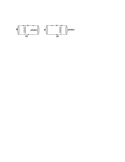
Figure 3: Diagrams of the contribution from hadronic structure of photon

In summary, combining all the NLP contributions together, we have

$$F_{V}^{NLP}(E_{\gamma}) = F_{V}^{NLP1}(E_{\gamma})+F_{V}^{NLP2}(E_{\gamma})+F_{V}^{NLP3}(E_{\gamma})+F_{V}^{NLP4}(E_{\gamma}),$$

$$F_{A}^{NLP}(E_{\gamma}) = F_{A}^{NLP1}(E_{\gamma})+F_{A}^{NLP2}(E_{\gamma})+F_{A}^{NLP3}(E_{\gamma})+F_{A}^{NLP4}(E_{\gamma}).$$ (44)

Based on the calculations in above sections, several comments are as follows:

• All the results of the form factors are given at tree level. The radiative corrections are of great importance in the hard exclusive processes, and in the $B\to\gamma l\nu$ decay it can reduce the leading order amplitude by $20\%-25\%$ in collinear factorization[32, 33, 34, 11]. In $k_{T}$ factorization, the NLO corrections have been studied in [19], while the endpoint behavior in this study is under controversy, and a more comprehensive study is required, which is left for a future study.

• For the contributions from higher twist $B$ meson wave functions up to twist-4, it has been found that it is free from endpoint singularity in the collinear factorization, thus the endpoint region is not very important and the Sudakov form factor and jet function is not essential. In addition, there is no study on the $k_{T}$ resummation effect for the higher twist wave functions so far, so the Sudakov factor is not considered here. If four-particle twist-5 and twist-6 wave functions are included, there does exist endpoint singularity[14], and the resummation effect must be considered.

• Only two-particle twist-2 and twist-3 photon LCDAs are employed in the contribution from the hadronic structure of photon. In [18], the contributions from the full set of photon LCDAs up to twist-4 are studied using light-cone sum rules approach, and the results indicate that the contribution from two-particle twist-2 LCDA is dominant, and the contribution from higher twist and three-particle LCDAs is suppressed. Here we neglect higher twist photon LCDAs except for two-particle twist-3 contribution which gives important contributions to the $B\to V$ form factors in the PQCD approach.

3 Numerical analysis

The most important input parameters are wave functions of $B$ meson and photon. We have assumed that the transverse momentum dependent $B$ meson wave function ${\phi}_{B}^{\pm}(x,k_{T})$ possesses the factorized form

$$\phi_{B}^{\pm}(x,k_{T})=\phi_{B}^{\pm}(x)\,\Sigma(k_{T})\,,$$ (45)

where the transverse part needs to be transformed into the impact parameter space through Fourier transform, and the wave functions turns to

$$\tilde{\phi}_{B}^{\pm}(x,b)=\phi_{B}^{\pm}(x)\,\tilde{\Sigma}(b)\,.$$ (46)

For the transverse part the Gaussian model is usually adopt in the PQCD approach, i.e. $\tilde{\Sigma}(b)=e^{-{1\over 2}\omega_{0}^{2}b^{2}}$, with $\omega_{0}=\lambda_{B}$. For the longitudinal part, we employ the following models to check the model dependence of the form factors. The first one is a free parton model[35]

$$\phi_{B\rm I}^{+}(x) = {x\over 2x_{1}^{2}}\,\theta(2x_{1}-x),$$

$$\phi_{B\rm I}^{-}(x) = {2x_{1}-x\over 2x_{1}^{2}}\,\theta(2x_{1}-x),$$ (47)

where $x_{1}=x_{0}=\omega_{0}/m_{B}$. The second one is from the QCD sum rules with local duality approximation[36]

$$\phi_{B\rm II}^{+}(x) = {3x\over 4x_{2}^{3}}\,(2x_{2}-x)\theta(2x_{2}-x),$$

$$\phi_{B\rm II}^{-}(x) = {1\over 8x_{2}^{3}}[3(2x_{2}-x)^{2}+{10(\lambda_{E}^{2}-\lambda_{H}^{2})\over 3x_{2}^{2}m_{B}^{2}}(3x^{2}-6xx_{2}+2x_{2}^{2})]\,\theta(2x_{2}-x),$$ (48)

where $x_{2}=3/2x_{0}$. In the phenomenological studies with PQCD approach, a more widely used model is as follows,

$$\phi_{B\rm III}^{+}(x) = \phi_{B\rm III}^{-}(x)=N_{B}x^{2}(1-x)^{2}e^{-{x^{2}\over 2x_{0}^{2}}},$$ (49)

where normalization constant $N_{B}$ is determined by $\lambda_{B}$. For the model of two-particle twist-4 $B$-meson LCDA, following [14] we adopt

$$\hat{g}^{+}_{B}(\omega) = {\omega^{2}\over 2\lambda_{B}}\bigg{(}1-{\lambda_{E}^{2}-\lambda_{H}^{2}\over 36\lambda_{B}^{2}}\bigg{)}e^{-{\omega\over\lambda_{B}}},$$ (50)

where the parameters $\lambda_{E}^{2}$ and $\lambda_{H}^{2}$ which are related to the matrix element of local quark-gluon operator can be estimated with QCD sum rules approach. The three-particle $B$ wave function is also supposed to satisfy $\psi(\omega,\xi,b,ub)=\psi(\omega,\xi)\tilde{\Sigma}(b)$, and the exponential model of the longitudinal part is widely used

$$\phi_{3}(\omega,\xi) = {\lambda_{E}^{2}-\lambda_{H}^{2}\over 6\lambda_{B}^{5}}\omega\xi^{2}e^{-{\omega+\xi\over\lambda_{B}}},$$

$$\psi_{4}(\omega,\xi) = {\lambda_{E}^{2}\over 3\lambda_{B}^{4}}\omega\xi e^{-{\omega+\xi\over\lambda_{B}}},$$

$$\tilde{\psi}_{4}(\omega,\xi) = {\lambda_{H}^{2}\over 3\lambda_{B}^{4}}\omega\xi e^{-{\omega+\xi\over\lambda_{B}}}.$$ (51)

The light-cone distribution amplitudes $\phi_{\gamma}(u),\psi^{(v,a)}(\omega,\xi)$ have been systematically studied in Ref.[37], and the expressions are quoted as follows. The two particle twist-2 LCDA is expanded in terms of Gegenbauer polynomials,

$$\phi_{\gamma}(u,\mu) = 6u\bar{u}\left[1+\sum_{n=2}^{\infty}b_{n}(\mu_{0})C^{3/2}_{n}(u-\bar{u})\right],$$ (52)

and twist-3 LCDAs in conformal expansion read

$$\psi^{(v)}(\xi,\mu) = 5\,\left(3\,\xi^{2}-1\right)+{3\over 64}\,\left[15\,\omega_{\gamma}^{V}(\mu)-5\,\omega_{\gamma}^{A}(\mu)\right]\,\left(3-30\,\xi^{2}+35\,\xi^{4}\right)\,,$$

$$\psi^{(a)}(\xi,\mu) = {5\over 2}\,\left(1-\xi^{2}\right)\,(5\,\xi^{2}-1)\left(1+{9\over 16}\,\omega_{\gamma}^{V}(\mu)-{3\over 16}\,\omega_{\gamma}^{A}(\mu)\right)\,.$$ (53)

In addition to the normalization constant(34,35), the scale dependence of the parameters in the LCDAs can be written as

$$b_{2}(\mu)=\left[{\alpha_{s}(\mu)\over\alpha_{s}(\mu_{0})}\right]^{8\over 33-2n_{f}}\,b_{2}(\mu_{0})\,,\qquad$$

$$\left(\begin{array}[]{c}\omega^{V}_{\gamma}(\mu)-\omega^{A}_{\gamma}(\mu)\\ \omega^{V}_{\gamma}(\mu)+\omega^{A}_{\gamma}(\mu)\end{array}\right)=\left({\alpha_{s}(\mu)\over\alpha_{s}(\mu_{0})}\right)^{\Gamma_{\omega}/\beta_{0}}\,\left(\begin{array}[]{c}\omega^{V}_{\gamma}(\mu_{0})-\omega^{A}_{\gamma}(\mu_{0})\\ \omega^{V}_{\gamma}(\mu_{0})+\omega^{A}_{\gamma}(\mu_{0})\end{array}\right)\,,$$ (58)

where the anomalous dimension matrix $\Gamma_{\omega}$ and $\beta_{0}$ is given by [37, 38]

$$\Gamma_{\omega} = \left(\begin{array}[]{c}3\,C_{F}-{2\over 3}\,C_{A}\qquad{2\over 3}\,C_{F}-{2\over 3}\,C_{A}\\ {5\over 3}\,C_{F}-{4\over 3}\,C_{A}\qquad{1\over 2}\,C_{F}+C_{A}\end{array}\right)\,,$$ (61)

$$\beta_{0} = 11-{2\over 3}n_{f}.$$ (62)

The value of the parameters used in the calculations are presented in Table(1), among them the scale dependent parameters are given at $\mu_{0}=1.0GeV$. These parameters should be run to the factorization scale $t$ in numerical analysis.

Table 1: Numerical value of the parameters entering the calculations

parameter	$\omega_{0}(\lambda_{B})$	$x_{0}$	$\chi(1GeV)$	$\langle\bar{q}q\rangle(1GeV)$
value	$0.35\pm 0.10GeV$	$0.076\pm 0.015$	$(3.15\pm 0.03)GeV^{-2}$	$-[(256^{+14}_{-16})MeV]^{3}$
parameter	$b_{2}(1GeV)$	$f_{3\gamma}(1GeV)$	$\omega^{V}_{\gamma}(1GeV)$	$\omega^{A}_{\gamma}(1GeV)$
value	$0.07\pm 0.07$	$-(4\pm 2)\times 10^{-3}\,{\rm GeV}^{2}$	$3.8\pm 1.8$	$-2.1\pm 1.0$
parameter	$N_{B}$	$\lambda_{E}^{2}$	$\lambda_{H}^{2}$	$f_{B}$
value	$3417$	$0.06\pm 0.04GeV^{2}$	$0.12\pm 0.05GeV^{2}$	$0.19\pm 0.02GeV$

Now we present the numerical results for the form factors $F_{V,A}$ and the branching ratio of $B\to\gamma\nu l$ decay. In physical interesting photon energy region $1.5GeV<E_{\gamma}<2.6GeV$, the leading power results of $F_{V,A}(E_{\gamma})$ at tree level are plotted in Fig(4), where all the parameters are fixed at the central values in Table(1). At leading power $F_{V}=F_{A}$ due to the left-handness of the standard model. The three curves are from the three models of leading twist $B$ meson wave functions, and the difference between them is only about $3\%-5\%$. In the following we set the model $\phi^{\pm}_{B\rm III}$ as default, which approaches zero at endpoint region. $\phi^{-}_{B\rm I,II}$ does not vanish when $x=0$, and it will lead to too large endpoint contribution when entering the factorization formula. Compared with the result of leading order $F_{V,A}$ in collinear factorization, the PQCD result is relatively smaller due to the inclusion of transverse momentum in the denominator of the propagators as well as suppression from $k_{T}$ resummation and threshold resummation.

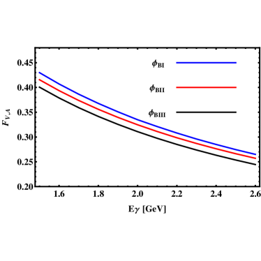
Figure 4: The leading power contribution to the form factors $F_{V,A}$, where blue,red and black curves are corresponding to the wave functions $\phi_{B\rm I}$,$\phi_{B\rm II}$ and $\phi_{B\rm III}$ respectively.

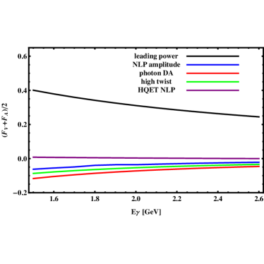
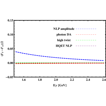
Figure 5: The next-to-leading power contribution to the form factors $F_{V,A}$. The left(right) panel denotes the photon momentum dependence of $(F_{V}+F_{A})/2$($(F_{V}-F_{A})/2$)respectively.

The NLP contribution to the form factors are presented in Fig(5). Among various kinds of contributions, which from hadronic structure of photon is most important. It decreases the leading power contribution by about $20\%$ for the symmetric form factor $(F_{V}+F_{A})/2$, and this result is consistent with the predictions from light-cone sum rules[18]. It can only give rise to a minor contribution to the symmetry breaking part $(F_{V}-F_{A})/2$ because the leading twist photon LCDA provides identical result for $F_{V}$ and $F_{A}$, and the symmetry breaking effect is only from higher twist photon LCDA . The contribution from higher twist $B$-meson wave functions, including both two-particle and three-particle Fock states, also decreases the leading power contribution by about $20\%$, and it keeps the symmetry between $F_{V}$ and $F_{A}$. The contribution from three particle $B$-meson wave functions is much smaller than that from higher twist two-particle wave function, which is consistent with the rough estimate in[20]. The power suppressed hard kernel can also give rise to sizeable corrections as the suppression factors $\omega/E_{\gamma}$ is not very small when $E_{\gamma}$ is not large. It is the main source of symmetry breaking part $(F_{V}-F_{A})/2$. The $1/m_{b}$ suppression term from HQET is negligible due to the cancellation between different part in Eq.(32). The different pieces of the NLP corrections considered in this paper are all sizable except for the $1/m_{b}$ suppression term from HQET, furthermore, the effects of them are all negative. The overall NLP correction is then significant, it decreases the LP result by about $50\%$. This result indicates the extraordinarily importance of power corrections in this channel.

Now we present the uncertainties from the various parameters in Table(1). If we fix $E_{\gamma}=2.0GeV$ and $\lambda_{B}=0.35GeV$, then the form factors with uncertainty are obtained as(in the unit of GeV)

$$F_{V}(2GeV)=0.169 + \bigg{(}^{+0.003}_{-0.003}\bigg{)}_{\lambda_{E}^{2}-\lambda_{H}^{2}}+\bigg{(}^{+0.020}_{-0.020}\bigg{)}_{f_{3\gamma}}+\bigg{(}^{+0.003}_{-0.003}\bigg{)}_{b_{2}}+\bigg{(}^{+0.011}_{-0.011}\bigg{)}_{\omega^{V}_{\gamma}}+\bigg{(}^{+0.002}_{-0.002}\bigg{)}_{\omega^{A}_{\gamma}}$$ (63)

$$+ \bigg{(}^{+0.018}_{-0.018}\bigg{)}_{f_{B}}+\bigg{(}^{+0.006}_{-0.006}\bigg{)}_{\langle\bar{q}q\rangle}+\bigg{(}^{+0.009}_{-0.012}\bigg{)}_{S_{t}}$$

$$F_{A}(2GeV)=0.135 + \bigg{(}^{+0.003}_{-0.003}\bigg{)}_{\lambda_{E}^{2}-\lambda_{H}^{2}}+\bigg{(}^{+0.018}_{-0.019}\bigg{)}_{f_{3\gamma}}+\bigg{(}^{+0.003}_{-0.003}\bigg{)}_{b_{2}}+\bigg{(}^{+0.008}_{-0.008}\bigg{)}_{\omega^{V}_{\gamma}}+\bigg{(}^{+0.001}_{-0.002}\bigg{)}_{\omega^{A}_{\gamma}}$$ (64)

$$+ \bigg{(}^{+0.015}_{-0.014}\bigg{)}_{f_{B}}+\bigg{(}^{+0.006}_{-0.006}\bigg{)}_{\langle\bar{q}q\rangle}+\bigg{(}^{+0.008}_{-0.011}\bigg{)}_{S_{t}}$$

where the important sources of the uncertainties include the parameters $f_{3\gamma}$ and $\omega_{V}$ in the distribution amplitude of photon, the decay constant of $B$ meson, and the parameter $c$ in the threshold resummation. For simplicity, $c(Q^{2})$ has been fixed as a constant and varies in the region $[0.45,0.65]$. Due to the variation regions of the twist-2 parameters $\chi(\mu_{0})$ and $\langle\bar{q}q\rangle$ are very small, the uncertainties from them are not important. The $E_{\gamma}$ dependence of the form factors with uncertainties is plotted in Fig.(6), where the errors are added in quadrature, and the overall uncertainty is expressed in the shaded region. Here the form factor $F_{A}$ is not shown for its uncertainty region is overlapped with $F_{V}$, instead, the uncertainty region of the symmetry breaking effect $(F_{V}-F_{A})/2$ is presented. The uncertainty region of $F_{V}$ is large because the parameters in the $B$ meson and photon wave functions are not well determined, and they should be constrained by more preciously measured physical quantities such as $B\to\pi$ transition form factors.

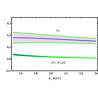
Figure 6: The form factors with uncertainty

Having the theoretical predictions of the form factors $F_{V,A}$ in our hands, we proceed to discuss the theory constraints on the first inverse moment $\lambda_{B}$ using integrated branching ratios of $B\to\gamma\nu l$. The lower limit of integral should be a photon-energy cut to get rid of the soft photon radiation. The integrated branching fractions with the phase-space cut on the photon energy read

$${\cal BR}(B\to\gamma\ell\nu,\,E_{\gamma}\geq E_{\rm cut})=\tau_{B}\,\int_{E_{\rm cut}}^{m_{B}/2}\,dE_{\gamma}\,{d\,\Gamma(B\to\gamma\ell\nu)\over d\,E_{\gamma}}\,,$$ (65)

where $\tau_{B}$ indicates the lifetime of the $B$-meson. Our predictions for the partial branching ratios of $B\to\gamma\ell\nu$ decay including power suppressed contributions are displayed in Fig.(7). The variation range of the first inverse moment $\lambda_{B}$ is $[0.25,0.45]\,{\rm GeV}$. It can be observed that the integrated branching fractions ${\cal BR}(B\to\gamma\ell\nu,\,E_{\gamma}\geq E_{\rm cut})$ grow with the decrease of $\lambda_{B}$, but the slope becomes small then $\lambda_{B}$ is getting large, in addition, the theoretical uncertainty is big. This $\lambda_{B}$ dependence behavior makes it more difficult to preciously determine the parameter $\lambda_{B}$. Recently, Belle collaboration reported their improved measurement of the branching ratio of $B\to\gamma\ell\nu$ with the energy cut $E_{\gamma}>1$GeV[39], the measured branching ratio is given by

$${\cal BR}(B\to\gamma\ell\nu,\,E_{\gamma}\geq{\rm 1.0GeV})=(1.4\pm 1.0\pm 0.4)\times 10^{-6}\,,$$ (66)

and a Bayesian upper limit of ${\cal BR}(B\to\gamma\ell\nu,\,E_{\gamma}\geq{\rm 1.0GeV})<3.0\times 10^{-6}\,$ is determined at 90% confidence level. Furthermore, the predictions and uncertainties of partial decay rate in Ref.[14] extrapolated to $E_{\gamma}>1$ GeV are used to determine $\lambda_{B}$. While if our result is employed, the uncertainty of $\lambda_{B}$ determined from $B\to\gamma\ell\nu$ decay should be larger. Thus a more systematic study of the NLP corrections to this channel is of great importance. On the experimental side, it is meaningful to measure the branching fraction with the phase-space cut on the photon energy larger than 1.5GeV, which is helpful to reduce model dependence.

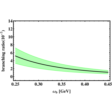
Figure 7: Dependence of the partial branching fractions ${\cal BR}(B\to\gamma\ell\nu,\,E_{\gamma}\geq E_{\rm cut})$ on the first inverse moment $\lambda_{B}(\mu_{0})$ for $E_{\rm cut}=1.5\,{\rm GeV}$ (blue band) and $E_{\rm cut}=2.0\,{\rm GeV}$ (green band).

4 CONCLUSION AND DISCUSSION

The leptonic radiative decay $B\to\gamma l\nu$ is believed to be an ideal channel to determine the $B$ meson wave functions, especially the first inverse moment $1/\lambda_{B}$, which is an important input in the semi-leptonic and non-leptonic $B$ meson decays. In the study of $B\to\gamma l\nu$ decay, the key problem is to investigate the form factors $F_{V,A}(E_{\gamma})$. We computed next-to-leading power corrections to the form factors within the framework of PQCD approach, including the power suppressed hard kernel, the contribution from a complete set of three-particle $B$ meson wave functions up to twist-4 and two particle off light-cone wave functions, the $1/m_{b}$ corrections in HQET, and the contribution from the hadronic structure of photon taking advantage of two-particle twist-2 and twist-3 photon LCDAs. In the study of power corrections, PQCD approach has its unique advantage because it is free from endpoint singularity through keeping transverse momentum of parton. Numerically, both the contribution from the higher twist $B$ meson wave functions and the hadronic structure of photon can reduce the leading power result by about $20\%$, and the power suppressed hard kernel decrease the leading power amplitude over $10\%$. The overall results is about $50\%$ smaller than leading power, under the condition that the QCD radiative corrections are not considered. Within the parameter space in this paper, the power correction is so important that one can hardly using the leading power result to reasonably determine the $B$ meson wave function. After including the power corrections, the integrated branching ratio of $B\to\gamma\nu l$ grows with decreasing $\lambda_{B}$, but the rate of change is smaller than the leading power case, in addition to the large theoretical uncertainty, it is difficult to preciously determine $\lambda_{B}$ only employing this processes. We should point out that our study is far from a systematic investigation, and more efforts need to be made to uncover the influence of the power corrections. With more and more precise measurements of $B\to\gamma l\nu$ decay, the parameters in $B$ meson wave functions must be better constrained.

References

[1] Y. Y. Keum, H. -n. Li, and A. I. Sanda,
Phys. Lett. B504, 6 (2001) [hep-ph/0004004];
Phys. Rev. D63, 054008 (2001) [hep-ph/0004173];
.
[2] C.-D. Lü, K. Ukai and M.-Z. Yang, Phys. Rev. D63, 074009
(2001) [hep-ph/0004213].
[3]
Qin Qin, Zhi-Tian Zou, Xin Yu, Hsiang-nan Li, C.-D. Lü, Phys. Lett. B 732 (2014), 36-40;
Shan Cheng, Qin Qin, arXiv:1810.10524 [hep-ph]; Xin Liu, Run-Hui Li, Zhi-Tian Zou, Zhen-Jun Xiao, Phys. Rev. D 96, 013005 (2017);
Zhi-Tian Zou, Ahmed Ali, C.-D. Lü, Xin Liu, and Ying Li, Phys. Rev. D 91 054033 (2015); Zhi-Tian Zou, Ying Li, and Xin Liu, Eur. Phys. J. C (2017) 77 870.
[4]
S. Nandi and H.-n. Li, Phys. Rev. D 76, 034008 (2007).
[5]
H.-n. Li and S. Mishima, Phys. Rev. D 80, 074024 (2009).
[6]
H.-n. Li, Y.-L. Shen, Y.-M. Wang, and H. Zou. Phys. Rev. D 83, 054029 (2011).
[7]
H. C. Hu and H. n. Li,
Phys. Lett. B 718, 1351 (2013)
doi:10.1016/j.physletb.2012.12.006
[arXiv:1204.6708 [hep-ph]].
[8]
S. Cheng, Y. Y. Fan and Z. J. Xiao,
Phys. Rev. D 89, no. 5, 054015 (2014)
doi:10.1103/PhysRevD.89.054015
[arXiv:1401.5118 [hep-ph]].
[9]
H. n. Li, Y. L. Shen and Y. M. Wang,
Phys. Rev. D 85, 074004 (2012)
doi:10.1103/PhysRevD.85.074004
[arXiv:1201.5066 [hep-ph]].
[10]
S. Cheng, Y. Y. Fan, X. Yu, C. D. Lü and Z. J. Xiao,
Phys. Rev. D 89, no. 9, 094004 (2014)
doi:10.1103/PhysRevD.89.094004
[arXiv:1402.5501 [hep-ph]].
[11]
M. Beneke and J. Rohrwild,
Eur. Phys. J. C 71 (2011) 1818
[arXiv:1110.3228 [hep-ph]].
[12]
V. M. Braun and A. Khodjamirian,
Phys. Lett. B 718 (2013) 1014
[arXiv:1210.4453 [hep-ph]].
[13]
Y. M. Wang,
JHEP 1609, 159 (2016)
doi:10.1007/JHEP09(2016)159
[arXiv:1606.03080 [hep-ph]].
[14]
M. Beneke, V. M. Braun, Y. Ji and Y. B. Wei,
JHEP 1807, 154 (2018)
doi:10.1007/JHEP07(2018)154
[arXiv:1804.04962 [hep-ph]].
[15]
C. W. Bauer, S. Fleming, D. Pirjol and I. W. Stewart,
Phys. Rev. D 63 (2001) 114020 [hep-ph/0011336].
C. W. Bauer and I. W. Stewart,
Phys. Lett. B 516 (2001) 134 [hep-ph/0107001].
[16]
M. Beneke, A. P. Chapovsky, M. Diehl and T. Feldmann,
Nucl. Phys. B 643 (2002) 431 [hep-ph/0206152];
M. Beneke and T. Feldmann,
Phys. Lett. B 553 (2003) 267 [hep-ph/0211358].
[17]
P. Ball and E. Kou,
JHEP 0304, 029 (2003)
doi:10.1088/1126-6708/2003/04/029
[hep-ph/0301135].
[18]
Y. M. Wang and Y. L. Shen,
JHEP 1805, 184 (2018)
[arXiv:1803.06667 [hep-ph]].
[19]
G. P. Korchemsky, D. Pirjol and T. M. Yan,
Phys. Rev. D 61 (2000) 114510
[hep-ph/9911427].
[20]
Y. Y. Charng and H. n. Li,
Phys. Rev. D 72, 014003 (2005)
doi:10.1103/PhysRevD.72.014003
[hep-ph/0505045].
[21]
J. P. Ma and Q. Wang,
JHEP 0601, 067 (2006)
doi:10.1088/1126-6708/2006/01/067
[hep-ph/0510336].
[22] S. Catani, M. Ciafaloni and F. Hautmann, Phys. Lett.
B 242, 97 (1990); Nucl. Phys. B 366, 135 (1991).
[23] J.C. Collins and R.K. Ellis, Nucl. Phys. B 360, 3 (1991).
[24] E.M. Levin, M.G. Ryskin, Yu.M. Shabelskii,
and A.G. Shuvaev, Sov. J. Nucl. Phys. 53, 657 (1991).
[25] J. Botts and G. Sterman, Nucl. Phys. B 325, 62 (1989).
[26] H.-n. Li and G. Sterman, Nucl. Phys. B 381, 129 (1992).
[27] M. Nagashima and H-n. Li, Phys. Rev. D 67,
034001 (2003).
[28] H-n. Li, hep-ph/0304217.
[29] T. Huang and Q.-X. Shen, Z. Phys. C 50, 139 (1991);
J.P. Ralston and B. Pire, Phys. Rev. Lett. 65, 2343 (1990);
R. Jakob and P. Kroll, Phys. Lett. B 315, 463 (1993); B 319, 545 (1993)(E).
[31]
H. N. Li, Y. L. Shen and Y. M. Wang,
JHEP 1302, 008 (2013)
doi:10.1007/JHEP02(2013)008
[arXiv:1210.2978 [hep-ph]].
[32]
S. Descotes-Genon and C. T. Sachrajda,
Nucl. Phys. B 650 (2003) 356
[hep-ph/0209216].
[33]
E. Lunghi, D. Pirjol and D. Wyler,
Nucl. Phys. B 649 (2003) 349
[hep-ph/0210091].
[34]
S. W. Bosch, R. J. Hill, B. O. Lange and M. Neubert,
Phys. Rev. D 67 (2003) 094014
[hep-ph/0301123].
[35] H. Kawamura, J. Kodaira, C.F. Qiao, and K. Tanaka,
Phys. Lett. B 523, 111 (2001); Erratum-ibid. 536, 344
(2002); Mod. Phys. Lett. A 18, 799 (2003).
[36]
V. M. Braun, D. Y. Ivanov and G. P. Korchemsky,
Phys. Rev. D 69, 034014 (2004)
doi:10.1103/PhysRevD.69.034014
[hep-ph/0309330].
[37]
P. Ball, V. M. Braun and N. Kivel,
Nucl. Phys. B 649, 263 (2003)
doi:10.1016/S0550-3213(02)01017-9
[hep-ph/0207307].
[38]
P. Ball, V. M. Braun, Y. Koike and K. Tanaka,
Nucl. Phys. B 529, 323 (1998)
doi:10.1016/S0550-3213(98)00356-3
[hep-ph/9802299].
[39]
M. Gelb et al. [Belle Collaboration],
arXiv:1810.12976 [hep-ex].