Analytic Network Learning

Abstract

Based on the property that solving the system of linear matrix equations via the column space and the row space projections boils down to an approximation in the least squares error sense, a formulation for learning the weight matrices of the multilayer network can be derived. By exploiting into the vast number of feasible solutions of these interdependent weight matrices, the learning can be performed analytically layer by layer without needing of gradient computation after an initialization. Possible initialization schemes include utilizing the data matrix as initial weights and random initialization. The study is followed by an investigation into the representation capability and the output variance of the learning scheme. An extensive experimentation on synthetic and real-world data sets validates its numerical feasibility.

Keywords: Multilayer Neural Networks, Least Squares Error, Linear Algebra, Deep Learning.

1 Introduction

1.1 Background

Attributed to its high learning capacity with good prediction capability, the deep neural network has found its advantage in wide areas of science and engineering applications. Such an observation has sparked a surge of investigations into the architectural and learning aspects of the deep network for targeted applications.

The main ground for realizing the high learning capacity and predictivity comes from several major advancements in the field which include the processing platform, the learning regimen, and the availability of big data size. In terms of the processing platform, the advancement in Graphics Processing Units (GPUs) has facilitated parallel processing of complex network learning within accessible time. Together with the relatively low cost of the hardware, the large number of public high level open source libraries has enabled a crowdsourcing mode of learning architectural exploration. Based on such a learning platform, several learning regimens such as the Convolutional Neural Network (CNN or LeNet-5) [1], the AlexNet [2], the GoogLeNet or Inception [3], the Visual Geometry Group Network (VGG Net) [4], the Residual Network (ResNet) [5] and the DenseNet [6] have stretched the network learning in terms of the network depth and prediction capability way beyond the known boundary established by the conventional statistical methods.

Without sufficiently convincing explanation in theory, the advancement of deep learning has been grounded upon ‘big’ data, powerful machinery and crowd efforts to achieve at ‘breakthrough’ results that were not possible before. Such a swarming phenomenon has pushed forward the demand of hardware as well as middle ware, but at the expense of masking the importance of fundamental results available in statistical decision theory. The research scene has arrived at such a state of deeming results unacceptable without working directly on or comparing them with ‘big’ data which implicitly relies on powerful machinery.

1.2 Motivation and Contributions

Despite the great success in applications, understanding of the underneath learning mechanism towards the representation and generalization properties gained from the network depth is being far fetched and becoming imperative. From the perspective of nonlinearity incurred by the activation functions in each layer, analyzing the learning properties of the network becomes extremely difficult.

In terms of the optimality of network learning, several investigations in the literature can be found. For the two-layer linear network, back in the year 1988, Baldi and Hornik [7, 8] showed that the network was convex in each of its two weight matrices and every local minimum was a global minimum. In 2012, Baldi and Lu [9] extended the result of convexity to deep linear network while conjecting that every local minimum was a global minimum. Recently, Kawaguchi [10] showed that the loss surface of deep linear networks was non-convex and non-concave, every local minimum was a global minimum, every critical point that was not a global minimum was a saddle point, and the rank of weight matrix at saddle points. These observations, represented in the form of Directed Acyclic Graph (DAG), were carried forward to the nonlinear networks with fewer unrealistic assumptions than that in [11, 12] which were inspired from the Hamiltonian of the spherical spin-glass model. Subsequently, Lu and Kawaguchi [13] showed that depth in linear networks created no bad local minima. More recently, Yun et al. [14] provided sufficient conditions for global optimality in deep nonlinear networks when the activation functions satisfied certain invertibility, differentiability and bounding conditions.

From the geometrical view of the loss function, Dinh et al. [15] argued that an appropriate definition and use of minima in terms of their sharpness could help in understanding the generalization behavior. With the understanding that the difficulty of deep search was originated from the proliferation of saddle points and not local minima, Dauphin et al. [16] attempted a saddle-free Newton’s method (see e.g., [17]) to search for the minima in deep networks. In [18], a visualization technique based on filter normalization was introduced for studying the loss landscape. By comparing networks with and without skip connections, the study showed that the smoothness of loss surface depended highly on the network architecture. The landscape of the empirical risk for deep learning of convolutional neural networks was investigated in [19]. By extending the case of linear networks in [20] to the case of nonlinear networks, Poggio et al. [21] showed that deep networks did not usually overfit the classification error for low-noise data sets and the solution corresponded to margin maximization.

From the view of having a theoretical bound for the estimation error, in 2002, Langford and Caruana [22] investigated into generalization in terms of the true error rate bound of a distribution over a set of neural networks using the PAC-Bayes bound. This approach had sparked off several follow-ups (see e.g., [23, 24, 25]). Recently, Bartlett et al. [26] proposed a margin-based generalization bound which was spectrally-normalized. Apart from an empirical investigation of several capacity bounds based on the $\ell_{2}$, $\ell_{1}$-path, $\ell_{2}$-path and the spectral norms [27], in [25], the margin-based perturbation bound was combined with the PAC-Bayes analysis to derive the generalization bound. Using the gap between the expected risk and the empirical risk, Kawaguchi et al. [28] provided generalization bounds for deep models which do not have explicit dependency on the number of weights, the depth and the input dimensionality. In view of the lack of an analytic structure in learning, many of these analyses were hinged upon the Stochastic Gradient Descent (SGD, see e.g.,[29, 30, 31]) search towards certain stationary points (e.g., [26, 19, 23, 24]). Moreover, many of the analyses of the linear network or the nonlinear one treated the network as a Directed Acyclic Graph (DAG) model (see e.g., [20, 24, 28]) where it turned into the complicated problem of topological sorting.

In [32, 33], we have established a gradient-free learning approach that results in an analytic learning of layered networks of fully connected structure. This simplifies largely the analytical aspects of network learning. In this work, we further explore the analytic learning on networks with receptive field. Particularly, the contributions of current study include (1) establishment of an analytic learning framework where its goal is to find a mapping matrix such that the target matrix falls within its range space. In other words, a representative mapping is sought after based on the data matrix and its Moore-Penrose inverse; (2) proposal of an analytic learning algorithm which utilizes the sparse structural information and showcase two initialization possibilities; (3) establishment of conditions for network representation on a finite set of data; (4) investigation of the network output variance with respect to the network depth; and (5) an extensive numerical study to validate the proposal.

1.3 Organization

The article is organized as follows. An introduction to several related concepts is given in Section 2 to pave the way for our development. Particularly, the Moore-Penrose inverse and its relation to least squares error approximation is defined and stated, together with the network structure of interest. Section 3 presents the main results of network learning in analytic form. Here, apart from a random initialization scheme, a deterministic initialization scheme based on the data matrix is introduced. This sheds some lights on the underlying learning mechanism. In Section 4, the issue of network representation is shown in view of a finite set of training data. The network generalization is further explored via the output variance of the linear structure. In Section 5, two cases of synthetic data are studied to observe the fitting behavior and the representation property of the proposed learning. In Section 6, the proposed learning is experimented on 42 data sets taken from the public domain to validate its numerical feasibility. Finally, some concluding remarks are given in Section 7.

2 Preliminaries

2.1 Moore-Penrose Inverse and Least Squares Solution

Definition 1

(see e.g., [34, 35, 36, 37]) A least squares solution to the system ${\bf A}{\boldsymbol{\theta}}={\bf y}$, where ${\bf A}\in\mbox{$\mathbb{R}$}^{m\times d}$, ${\boldsymbol{\theta}}\in\mbox{$\mathbb{R}$}^{d\times 1}$ and ${\bf y}\in\mbox{$\mathbb{R}$}^{m\times 1}$, is a vector $\hat{\boldsymbol{\theta}}$ such that

$$\|\hat{\bf e}\|=\|{\bf A}\hat{\boldsymbol{\theta}}-{\bf y}\|\leqslant\|{\bf A}{\boldsymbol{\theta}}-{\bf y}\|=\|{\bf e}\|,$$ (1)

where $\|\cdot\|$ denotes the $\ell^{2}$-norm of “$\cdot$”.

Definition 2

(see e.g., [36, 34, 35, 37]) If ${\bf A}$ (square or rectangular) is a matrix of real or complex elements, then there exits a unique matrix ${\bf A}^{{\dagger}}$, known as the Moore-Penrose inverse or the pseudoinverse of ${\bf A}$, such that (i) ${\bf A}{\bf A}^{{\dagger}}{\bf A}={\bf A}$, (ii) ${\bf A}^{{\dagger}}{\bf A}{\bf A}^{{\dagger}}={\bf A}^{{\dagger}}$, (iii) $({\bf A}{\bf A}^{{\dagger}})^{*}={\bf A}{\bf A}^{{\dagger}}$ and (iv) $({\bf A}^{{\dagger}}{\bf A})^{*}={\bf A}^{{\dagger}}{\bf A}$ where ^∗ denotes the conjugate transpose.

Lemma 1

(see e.g., [35, 34, 36, 37]) $\hat{\boldsymbol{\theta}}={\bf A}^{{\dagger}}{\bf y}$ is the best approximate solution of ${\bf A}{\boldsymbol{\theta}}={\bf y}$.

If the linear system of equations ${\bf A}{\boldsymbol{\theta}}={\bf y}$ is an over-determined one (i.e., $m>d$) and the columns of ${\bf A}$ are linearly independent, then ${\bf A}^{{\dagger}}=({\bf A}^{T}{\bf A})^{-1}{\bf A}^{T}$ and ${\bf A}^{{\dagger}}{\bf A}={\bf I}$. The solution to the system can be derived via pre-multiplying ${\bf A}^{{\dagger}}$ to both sides of ${\bf A}{\boldsymbol{\theta}}={\bf y}$ giving ${\bf A}^{{\dagger}}{\bf A}\hat{\boldsymbol{\theta}}={\bf A}^{{\dagger}}{\bf y}$ which leads to the result in Lemma 1 since ${\bf A}^{{\dagger}}{\bf A}={\bf I}$. On the other hand, if ${\bf A}{\boldsymbol{\theta}}={\bf y}$ is an under-determined system (i.e., $m<d$) and the rows of ${\bf A}$ are linearly independent, then ${\bf A}^{{\dagger}}={\bf A}^{T}({\bf A}{\bf A}^{T})^{-1}$ and ${\bf A}{\bf A}^{{\dagger}}={\bf I}$. Here, the solution to the system can be derived by substituting $\hat{\boldsymbol{\theta}}={\bf A}^{{\dagger}}\hat{\boldsymbol{\alpha}}$ (a projection of $d$ space onto the $m$ subspace) into the system and then solve for $\hat{\boldsymbol{\alpha}}\in\mbox{$\mathbb{R}$}^{m}$ which results in $\hat{\boldsymbol{\alpha}}={\bf y}$. The result in Lemma 1 is again obtained by substituting $\hat{\boldsymbol{\alpha}}={\bf y}$ into $\hat{\boldsymbol{\theta}}={\bf A}^{{\dagger}}\hat{\boldsymbol{\alpha}}$. In practice, the full rank condition may not be easily achieved for data with large dimension without regularization. For such cases, the Moore-Penrose inverse in Definition 2 exists and is unique. This means that for any matrix ${\bf A}$, there is precisely one matrix ${\bf A}^{{\dagger}}$ that satisfies the four properties of the Penrose equations in Definition 2. In general, if ${\bf A}$ has a full rank factorization such that ${\bf A}={\bf F}{\bf G}$, then ${\bf X}^{{\dagger}}={\bf G}^{*}({\bf G}{\bf G}^{*})^{-1}({\bf F}^{*}{\bf F})^{-1}{\bf F}^{*}$ satisfies the Penrose equations [36].

The above algebraic relationships show that learning of a linear system in the sense of least squares error minimization can be achieved by manipulating its kernel or the range space via the Moore-Penrose inverse operation (i.e., multiplying the pseudoinverse of a system matrix to both sides of the equation boils down to an implicit least squares error minimization, the readers are referred to [33] for greater details regarding the least error and the least norm properties). For linear systems with multiple ($q$) output columns, the following result is observed.

Lemma 2

[32] Solving for $\boldsymbol{\Theta}$ in the system of linear equations of the form

$${\bf A}\boldsymbol{\Theta}={\bf Y},\ \ \ {\bf A}\in\mbox{$\mathbb{R}$}^{m\times d},\ \boldsymbol{\Theta}\in\mbox{$\mathbb{R}$}^{d\times q},\ {\bf Y}\in\mbox{$\mathbb{R}$}^{m\times q}$$ (2)

in the column space (range) of ${\bf A}$ or in the row space (kernel) of ${\bf A}$ is equivalent to minimizing the sum of squared errors given by

$$\textup{SSE}=trace\left(({\bf A}\boldsymbol{\Theta}-{\bf Y})^{T}({\bf A}\boldsymbol{\Theta}-{\bf Y})\right).$$ (3)

Moreover, the resultant solution $\hat{\boldsymbol{\Theta}}={\bf A}^{{\dagger}}{\bf Y}$ is unique with a minimum-norm value in the sense that $\|\hat{\boldsymbol{\Theta}}\|^{2}_{2}\leqslant\|\boldsymbol{\Theta}\|^{2}_{2}$ for all feasible $\boldsymbol{\Theta}$.

Proof: Equation (2) can be re-written as a set of multiple linear systems as follows:

$${\bf A}[\boldsymbol{\theta}_{1},\cdots,\boldsymbol{\theta}_{q}]=[{\bf y}_{1},\cdots,{\bf y}_{q}].$$ (4)

Since the trace of $({\bf A}\boldsymbol{\Theta}-{\bf Y})^{T}({\bf A}\boldsymbol{\Theta}-{\bf Y})$ is equal to the sum of the squared lengths of the error vectors ${\bf A}\boldsymbol{\theta}_{i}-{\bf y}_{i}$, $i=1,2,...,q$, the unique solution $\hat{\boldsymbol{\Theta}}=({\bf A}^{T}{\bf A})^{-1}{\bf A}^{T}{\bf Y}$ in the column space of ${\bf A}$ or that $\hat{\boldsymbol{\Theta}}={\bf A}^{T}({\bf A}{\bf A}^{T})^{-1}{\bf Y}$ in the row space of ${\bf A}$, not only minimizes this sum, but also minimizes each term in the sum [38]. Moreover, since the column and the row spaces are independent, the sum of the individually minimized norms is also minimum.  $\blacksquare$

Based on these observations, the inherent least squares error approximation property of algebraic manipulation utilizing the Moore-Penrose inverse shall be exploited in the following section to derive an analytic solution for multilayer network learning that is gradient-free.

2.2 Feedforward Neural Network

We consider a multilayer feedforward network of $n$ layers. This network can either be fully connected or with a receptive field setting (also known as a receptive field network, we abbreviated it as RFN hereon) as shown in Fig. 1. When a full receptive field is set for all layers, the network is a fully connected one [32, 33]. Unlike conventional networks, the bias term in each layer is excluded except for the inputs in this representation.

Mathematically, the $n$-layer network model of $h_{1}$-$h_{1}$-$\cdots$-$h_{n-1}$-$h_{n}$ structure can be written in matrix form as

$${\bf G}=f_{n}\left(f_{n-1}(\cdots f_{2}(f_{1}({\bf X}{\bf W}_{1}){\bf W}_{2})\cdots{\bf W}_{n-1}){\bf W}_{n}\right),$$ (5)

where ${\bf X}=[{\bf 1},\boldsymbol{X}]\in\mbox{$\mathbb{R}$}^{m\times(d+1)}$ is the augmented input data matrix (i.e., input with bias), ${\bf W}_{1}\in\mbox{$\mathbb{R}$}^{(d+1)\times h_{1}}$, ${\bf W}_{2}\in\mbox{$\mathbb{R}$}^{h_{1}\times h_{2}}$, $\cdots$, ${\bf W}_{n-1}\in\mbox{$\mathbb{R}$}^{h_{n-2}\times h_{n-1}}$, and ${\bf W}_{n}\in\mbox{$\mathbb{R}$}^{h_{n-1}\times q}$ ($h_{n}=q$ is the output dimension) are the weight matrices without bias at each layer, and ${\bf G}\in\mbox{$\mathbb{R}$}^{m\times q}$ is the network output of $q$ dimension. $f_{k}$, $k=1,\cdots,n$ are activation functions which operate elementwise on its matrix domain. When the $k^{th}$ layer of the network has a limited receptive field, then its weight matrix has sparse elements in each column. For example, if the first layer has receptive field of $3$ (denoted as $r_{3}$), then, when $h_{1}=d$, ${\bf W}_{1}$ can be written as a circulant matrix [39, 40] as follows:

$$\hskip 65.44142pth_{1}=d$$

$${\bf W}_{1} = \overbrace{\left[\begin{array}[]{ccccc}w_{1,1}&0&0&\cdots&0\\ w_{2,1}&w_{2,2}&0&\cdots&0\\ w_{3,1}&w_{3,2}&w_{3,3}&\cdots&0\\ 0&w_{4,2}&w_{4,3}&\cdots&0\\ 0&0&w_{5,3}&\cdots&0\\ 0&0&0&\cdots&0\\ 0&0&0&\ddots&w_{d-1,d}\\ 0&0&0&\cdots&w_{d,d}\\ 0&0&0&\cdots&w_{d+1,d}\\ \end{array}\right]}.$$ (15)

For simplicity, the activation functions in each layer are taken to be the same (i.e., $f_{k}=f$, $k=1,\cdots,n$) in our development. Also, unless stated otherwise, all activation functions are taken to operate elementwise on its matrix domain. We shall denote this network with receptive field as one with structure $h_{1}^{r_{3}}$-$h_{2}$-$\cdots$-$h_{n-1}$-$h_{n}$ which carries the common activation function in each layer of $f(h_{1}^{r_{3}})$-$f(h_{2})$-$\cdots$-$f(h_{n-1})$-$f(h_{n})$.

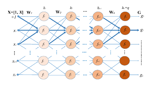
Figure 1: An $n$-layer feedforward network without inner weight biases.

2.3 Invertible Function

In some circumstances, we may need to invert the network over the activation function for solution seeking. For such a case, an inversion is performed through a functional inversion. The inverse function is defined as follows.

Definition 3

Consider a function $f$ which maps $x\in\mbox{$\mathbb{R}$}$ to $y\in\mbox{$\mathbb{R}$}$, i.e., $y=f(x)$. Then the inverse function for $f$ is such that $f^{-1}(y)=x$.

A good example for invertible function is the softplus function given by $y=f(x)=\log(1+e^{x})$ and its inverse given by $\log(e^{y}-1)$. Although other invertible functions can be used, this function and its modified versions, shall be adopted in all our experiments for illustration purpose.

3 Network Learning

The indexing of $f_{k}$, $k=1,\cdots,n$ for each layer of (5) is kept here for clarity purpose and suppose $f_{k}=f$ is an invertible function. Then, the network can learn a given target matrix ${\bf Y}\in\mbox{$\mathbb{R}$}^{m\times q}$ by putting ${\bf G}={\bf Y}$ where each layer of the network can be inverted (via taking functional inverse and pseudoinverse) as follows:

$${\bf Y}=f_{n}\left(f_{n-1}(f_{n-2}(\cdots f_{2}(f_{1}({\bf X}{\bf W}_{1}){\bf W}_{2})\cdots){\bf W}_{n-1}){\bf W}_{n}\right)$$

$$\Rightarrow f^{-1}_{n}({\bf Y})=f_{n-1}(f_{n-2}(\cdots f_{2}(f_{1}({\bf X}{\bf W}_{1}){\bf W}_{2})\cdots){\bf W}_{n-1}){\bf W}_{n}$$

$$\Rightarrow f^{-1}_{n}({\bf Y}){\bf W}_{n}^{{\dagger}}=f_{n-1}(f_{n-2}(\cdots f_{2}(f_{1}({\bf X}{\bf W}_{1}){\bf W}_{2})\cdots){\bf W}_{n-1})$$

$$\Rightarrow f^{-1}_{n-1}({f^{-1}_{n}({\bf Y})\bf W}_{n}^{{\dagger}})=f_{n-2}(\cdots f_{2}(f_{1}({\bf X}{\bf W}_{1}){\bf W}_{2})\cdots){\bf W}_{n-1}$$

$$\Rightarrow \vdots$$

$$\Rightarrow f^{-1}_{2}(\cdots f^{-1}_{n-1}(f^{-1}_{n}({\bf Y}){\bf W}_{n}^{{\dagger}}){\bf W}_{n-1}^{{\dagger}}\cdots)=f_{1}({\bf X}{\bf W}_{1}){\bf W}_{2}$$ (18)

$$\Rightarrow f^{-1}_{1}(f^{-1}_{2}(\cdots f^{-1}_{n-1}(f^{-1}_{n}({\bf Y}){\bf W}_{n}^{{\dagger}}){\bf W}_{n-1}^{{\dagger}}\cdots){\bf W}_{2}^{{\dagger}})={\bf X}{\bf W}_{1}.$$ (19)

Based on (3) to (19), we can express the weight matrices respectively as

$${\bf W}_{1} = {\bf X}^{{\dagger}}f^{-1}_{1}(f^{-1}_{2}(f^{-1}_{3}(\cdots f^{-1}_{n-1}(f^{-1}_{n}({\bf Y}){\bf W}_{n}^{{\dagger}}){\bf W}_{n-1}^{{\dagger}}\cdots){\bf W}_{3}^{{\dagger}}){\bf W}_{2}^{{\dagger}})$$ (20)

$${\bf W}_{2} = [f_{1}({\bf X}{\bf W}_{1})]^{{\dagger}}f^{-1}_{2}(f^{-1}_{3}(\cdots f^{-1}_{n-1}(f^{-1}_{n}({\bf Y}){\bf W}_{n}^{{\dagger}}){\bf W}_{n-1}^{{\dagger}}\cdots){\bf W}_{3}^{{\dagger}})$$

$$\vdots$$

$${\bf W}_{n-1} = [f_{n-2}(\cdots f_{2}(f_{1}({\bf X}{\bf W}_{1}){\bf W}_{2})\cdots{\bf W}_{n-2})]^{{\dagger}}f^{-1}_{n-1}(f^{-1}_{n}({\bf Y}){\bf W}_{n}^{{\dagger}})$$

$${\bf W}_{n} = [f_{n-1}(f_{n-2}(\cdots f_{2}(f_{1}({\bf X}{\bf W}_{1}){\bf W}_{2})\cdots){\bf W}_{n-1})]^{{\dagger}}f^{-1}_{n}({\bf Y}).$$ (23)

With these derivations, the follow result is stated formally.

Theorem 1

Given $m$ data samples of $d$ dimension which are packed as ${\bf X}\in\mbox{$\mathbb{R}$}^{m\times(d+1)}$ with augmentation, and consider a multilayer network of the form in (5) with $f_{k}=f$, $\forall k=1,\cdots,n$ being invertible. Then, learning of the network towards the target ${\bf Y}\in\mbox{$\mathbb{R}$}^{m\times q}$ in the sense of least squares error approximation boils down to solving the set of equations given by (20) through (23).

Proof: Since the Moore-Penrose inverse exists uniquely for any complex or real matrix and the activation functions are invertible, the results follow directly the derivations in (3) through (20). The assertion of least squares error approximation comes from the observation in Lemma 2 where each step of manipulating each equation (in (3) through (20)) by taking the pseudoinverse implies a projection onto either the column space or the row space. Mathematically, suppose ${\bf A}=f_{n-1}(f_{n-2}(\cdots f_{2}(f_{1}({\bf X}{\bf W}_{1}){\bf W}_{2})\cdots){\bf W}_{n-1})$. Then (23) can be rewritten as ${\bf W}_{n}={\bf A}^{{\dagger}}f^{-1}_{n}({\bf Y})$. The least squares approximation property can be easily visualized by substituting (23) into (5) to get ${\bf G}=f_{n}({\bf A}{\bf W}_{n})=f_{n}({\bf A}{\bf A}^{{\dagger}}f^{-1}_{n}({\bf Y}))$. By taking $f^{-1}_{n}$ to both sides of the equation, we have $f^{-1}_{n}({\bf G})={\bf A}{\bf A}^{{\dagger}}f^{-1}_{n}({\bf Y})$. Considering each column of the equation given by $f^{-1}_{n}({\bf g})={\bf A}{\bf A}^{{\dagger}}f^{-1}_{n}({\bf y})$, we observe the analogue to $\hat{\bf y}={\bf A}\hat{\boldsymbol{\theta}}={\bf A}{\bf A}^{{\dagger}}{\bf y}$ of Lemma 1 by putting ${\bf g}=\hat{\bf y}$ where the invertible transform of the target $f^{-1}_{n}({\bf y})$ can be recovered uniquely. Hence the proof.  $\blacksquare$

The above result shows that the least squares solution to the network weights comes in a cross-coupling form where the weight matrices are interdependent. This poses difficulty towards an analytical estimation. Fortunately, due to the high redundancy of the network weights that are constrained within an array structure, the solutions to network learning are vastly available (see section 4.2 for a detailed analysis). The following result is obtained by having the weight matrices ${\bf W}_{k}$, $k=2,\cdots,n$ arbitrarily initialized as non-trivial matrices ${\bf R}_{k}$, $k=2,\cdots,n$ (e.g., a matrix which has zero value for all its elements is considered a trivial matrix).

Corollary 1

Consider $m$ data samples of $d$ dimension which are packed as ${\bf X}\in\mbox{$\mathbb{R}$}^{m\times(d+1)}$ with augmentation. Given non-trivial matrices ${\bf R}_{i}$, $i=2,\cdots,n$ where their dimensions matches those of ${\bf W}_{j}$, $j=2,\cdots,n$ in (5) and suppose the activation functions are invertible. Then, learning of the network towards the target ${\bf Y}\in\mbox{$\mathbb{R}$}^{m\times q}$ admits the following solution to the least squares error approximation:

$${\bf W}_{1} = {\bf X}^{{\dagger}}f^{-1}_{1}(f^{-1}_{2}(f^{-1}_{3}(\cdots f^{-1}_{n-1}(f^{-1}_{n}({\bf Y}){\bf R}_{n}^{{\dagger}}){\bf R}_{n-1}^{{\dagger}}\cdots){\bf R}_{3}^{{\dagger}}){\bf R}_{2}^{{\dagger}})$$ (24)

$${\bf W}_{2} = [f_{1}({\bf X}{\bf W}_{1})]^{{\dagger}}f^{-1}_{2}(f^{-1}_{3}(\cdots f^{-1}_{n-1}(f^{-1}_{n}({\bf Y}){\bf R}_{n}^{{\dagger}}){\bf R}_{n-1}^{{\dagger}}\cdots){\bf R}_{3}^{{\dagger}})$$

$$\vdots$$

$${\bf W}_{n-1} = [f_{n-2}(\cdots f_{2}(f_{1}({\bf X}{\bf W}_{1}){\bf W}_{2})\cdots)]^{{\dagger}}f^{-1}_{n-1}(f^{-1}_{n}({\bf Y}){\bf R}_{n}^{{\dagger}})$$ (26)

$${\bf W}_{n} = [f_{n-1}(f_{n-2}(\cdots f_{2}(f_{1}({\bf X}{\bf W}_{1}){\bf W}_{2})\cdots){\bf W}_{n-1})]^{{\dagger}}f^{-1}_{n}({\bf Y}).$$ (27)

Proof: By initializing the weights ${\bf W}_{j}$, $j=2,\cdots,n$ using matrices ${\bf R}_{i}$, $i=2,\cdots,n$, the inter-dependency of weights can be decoupled and the weights can be estimated sequentially from (24) to (27). Hence the proof.  $\blacksquare$

Corollary 2

Consider $m$ data samples of $d$ dimension which are packed as ${\bf X}\in\mbox{$\mathbb{R}$}^{m\times(d+1)}$ with augmentation. Given non-trivial matrices ${\bf R}_{i}$, $i=1,2,4,5\cdots,n$ where their dimensions matches those of ${\bf W}_{j}$, $j=1,2,4,5\cdots,n$ in (5) and suppose the activation functions are invertible. Then, learning of the network towards the target ${\bf Y}\in\mbox{$\mathbb{R}$}^{m\times q}$ admits the following solution to the least squares error approximation:

$${\bf W}_{3} = [f_{2}(f_{1}({\bf X}{\bf R}_{1}){\bf R}_{2})]^{{\dagger}}f^{-1}_{3}(f^{-1}_{4}(f^{-1}_{5}(\cdots f^{-1}_{n-1}(f^{-1}_{n}({\bf Y}){\bf R}_{n}^{{\dagger}}){\bf R}_{n-1}^{{\dagger}}\cdots){\bf R}_{5}^{{\dagger}}){\bf R}_{4}^{{\dagger}})$$

$${\bf W}_{4} = [f_{3}(f_{2}(f_{1}({\bf X}{\bf R}_{1}){\bf R}_{2}){\bf W}_{3})]^{{\dagger}}f^{-1}_{4}(f^{-1}_{5}(\cdots f^{-1}_{n-1}(f^{-1}_{n}({\bf Y}){\bf R}_{n}^{{\dagger}}){\bf R}_{n-1}^{{\dagger}}\cdots){\bf R}_{5}^{{\dagger}})$$

$$\vdots$$

$${\bf W}_{n-1} = [f_{n-2}(\cdots f_{3}(f_{2}(f_{1}({\bf X}{\bf R}_{1}){\bf R}_{2}){\bf W}_{3})\cdots{\bf W}_{n-2})]^{{\dagger}}f^{-1}_{n-1}(f^{-1}_{n}({\bf Y}){\bf R}_{n}^{{\dagger}})$$ (30)

$${\bf W}_{1} = {\bf X}^{{\dagger}}f^{-1}_{1}(f^{-1}_{2}(f^{-1}_{3}(\cdots f^{-1}_{n-1}(f^{-1}_{n}({\bf Y}){\bf R}_{n}^{{\dagger}}){\bf W}_{n-1}^{{\dagger}}\cdots){\bf W}_{3}^{{\dagger}}){\bf R}_{2}^{{\dagger}})$$ (31)

$${\bf W}_{2} = [f_{1}({\bf X}{\bf W}_{1})]^{{\dagger}}f^{-1}_{2}(f^{-1}_{3}(\cdots f^{-1}_{n-1}(f^{-1}_{n}({\bf Y}){\bf R}_{n}^{{\dagger}}){\bf W}_{n-1}^{{\dagger}}\cdots){\bf W}_{3}^{{\dagger}})$$ (32)

$${\bf W}_{n} = [f_{n-1}(f_{n-2}(\cdots f_{3}(f_{2}(f_{1}({\bf X}{\bf W}_{1}){\bf W}_{2}){\bf W}_{3})\cdots){\bf W}_{n-1})]^{{\dagger}}f^{-1}_{n}({\bf Y}).$$ (33)

Proof: The order of learning sequence is immaterial for any of the inner layer weights ${\bf W}_{i}$, $i=1,2,4,\cdots,n-1$, but the output layer weight ${\bf W}_{n}$ should be lastly estimated. This is because ${\bf W}_{n}$ is the weight which links up all hidden layer weights and provides a direct least squares error approximation (range space projection) to the target ${\bf Y}$. In other words, the estimation of ${\bf W}_{n}$ (33) at the output layer is complete when all the hidden weights have been determined. Hence the proof.  $\blacksquare$

Apart from the above solution based on random initialization, the following result shows an example of non-random initialization. This is particularly useful when the activation functions are non-invertible.

Corollary 3

Given $m$ data samples of $d$ dimension which are packed as ${\bf X}\in\mbox{$\mathbb{R}$}^{m\times(d+1)}$ with augmentation. Then, learning of the network (5) towards the target ${\bf Y}\in\mbox{$\mathbb{R}$}^{m\times q}$ admits the following solution to the least squares error approximation:

$${\bf W}_{1} = {\bf X}^{{\dagger}}$$ (34)

$${\bf W}_{2} = [f_{1}({\bf X}{\bf W}_{1})]^{{\dagger}}$$

$$\vdots$$

$${\bf W}_{n-1} = [f_{n-2}(\cdots f_{2}(f_{1}({\bf X}{\bf W}_{1}){\bf W}_{2})\cdots)]^{{\dagger}}$$ (36)

$${\bf W}_{n} = [f_{n-1}(f_{n-2}(\cdots f_{2}(f_{1}({\bf X}{\bf W}_{1}){\bf W}_{2})\cdots){\bf W}_{n-1})]^{{\dagger}}f^{-1}_{n}({\bf Y}).$$ (37)

Proof: Since ${\bf R}_{i}$, $i=2,\cdots,n$ in Corollary 1 are arbitrarily assigned matrices that matches the dimensions of the corresponding weight matrices, they, together with $f^{-1}_{i}$, $i=1,\cdots,n$ on ${\bf Y}$ are indeed arbitrary, and they all can be chosen as identity matrix as one particular solution. Since the estimation of the output weight matrix ${\bf W}_{n}$ in (27) of Corollary 1 does not involve assignment of the arbitrary matrix ${\bf R}_{i}$, the transformed target term $f^{-1}_{n}({\bf Y})$ cannot be replaced by the identity matrix. Hence the proof.  $\blacksquare$

Remark 1: The result in Corollary 1 shows that there exits an infinite number of solutions for a network with multiple layers due to the arbitrary weight initialization. However, this does not apply to the single layer network because it can be reduced to the system of linear equations. The result in Corollary 2 shows that the sequence of weights estimation need not begin from the first layer. Indeed, the arbitrary weights in Corollary 1 and Corollary 2 are only utilized once following the sequence of weight matrix estimation. The weight matrix after each step of the estimation sequence is no longer arbitrary because all the previously estimated weights are used in the subsequent pseudoinverse projection towards the least squared error approximation. Corollary 3 shows a particular choice of the arbitrary weight matrix assignment without needing the corresponding activation functions to be invertible. For non-invertible functions, the term $f^{-1}_{n}({\bf Y})$ in (37) can be replaced by ${\bf Y}$ which corresponds to a linear output layer in (5). However, such an identity setting results in having the number of network nodes in every hidden layer (i.e., $h_{i}$, the column size of ${\bf W}_{i}$, $i=1,\cdots,n-1$) being set equal to the sample size $m$.  $\square$

The proposed algorithms in Corollary 1 through Corollary 3 are differentiated from that in [8] in several ways. Firstly, the nonlinear activation function was not considered in [8] whereas in our approach, nonlinear activations, both invertible and not, are considered. Secondly, in Corollary 1 through Corollary 3, there is no attempt to alternate the search of weights among the layers as that in [8] since such a search leads to the convergence issue. Lastly but not the least, we capitalize on the powerful Moore-Penrose inverse for solving the weights. More importantly, the layered network learning solution becomes analytical after arriving at (37) (and so are (27) and (33)), i.e., the problem boils down to finding an input correlated matrix $f_{n-1}(f_{n-2}(\cdots f_{2}(f_{1}({\bf X}{\bf W}_{1}){\bf W}_{2})\cdots){\bf W}_{n-1})$ that can represent ${\bf Y}$. This can be seen by considering a network with linear output where ${\bf G}=f_{n-1}({\bf A}_{n-1}){\bf W}_{n}$ with ${\bf A}_{n-1}=f_{n-2}({\bf A}_{n-2}){\bf W}_{n-1}$, $\cdots$, ${\bf A}_{1}={\bf X}{\bf W}_{1}$. When the learning is based on Corollary 3 where ${\bf W}_{1}={\bf X}^{{\dagger}}$, ${\bf W}_{2}=[f_{1}({\bf A}_{1})]^{{\dagger}}$, $\cdots$, ${\bf W}_{n}=[f_{n-1}({\bf A}_{n-1})]^{{\dagger}}{\bf Y}$, then we have the estimated output given by

$$\hat{\bf Y}=f_{n-1}({\bf A}_{n-1})[f_{n-1}({\bf A}_{n-1})]^{{\dagger}}{\bf Y},$$ (38)

where ${\bf A}_{n-1}=f_{n-2}({\bf A}_{n-2})[f_{n-2}({\bf A}_{n-2})]^{{\dagger}}$, $\cdots$, ${\bf A}_{1}={\bf X}{\bf X}^{{\dagger}}$. This shows that each layer in (38) serves as a composition of projection bases, based on the data matrix or the transformed data matrix (transformed by $f_{k}$, $k=1,\cdots,n-1$), to hold the target ${\bf Y}$ within its range. In a nutshell, our results show that the problem of network learning can be viewed as one to find a data mapping matrix such that the target matrix falls within its range. An immediate advantage of such a view over the conventional view of error minimization is evident from the gradient-free solutions arrived in Corollaries 1–3. These results shall be validated by numerical evaluations in the experimental section.

4 Network Representation and Generalization

Firstly, we show the network representation capability. Then, an analysis of the feasible solution space is presented. Finally, an analysis of the output variance is performed.

4.1 Network Representation

For simplicity, we shall use $d$ as the dimension for generic matrices instead of the augmented dimension $d+1$ when no ambiguity arises.

Definition 4

A matrix ${\bf A}\in\mbox{$\mathbb{R}$}^{m\times d}$ is said to be representative for ${\bf Y}\in\mbox{$\mathbb{R}$}^{m\times q}$ if ${\bf A}{\bf A}^{{\dagger}}{\bf Y}={\bf Y}$ where $m,d,q\geqslant 1$.

Certainly, if ${\bf A}$ has full rank in the sense that ${\bf A}{\bf A}^{T}$ is invertible for ${\bf A}^{{\dagger}}={\bf A}^{T}({\bf A}{\bf A}^{T})^{-1}$, then ${\bf A}{\bf A}^{{\dagger}}={\bf I}$ for which ${\bf A}$ is representative for ${\bf Y}$. However, this definition of representation is weaker than the full rank requirement in $({\bf A}^{T}{\bf A})^{-1}{\bf A}^{T}$ or ${\bf A}^{T}({\bf A}{\bf A}^{T})^{-1}$ because ${\bf A}$ needs not have full rank when ${\bf Y}$ falls within the range of ${\bf A}$.

Definition 5

A function $f$, which operates elementwise on its matrix domain, is said to be representative if $f({\bf X}{\bf W}_{1})$ is representative for ${\bf Y}\in\mbox{$\mathbb{R}$}^{m\times q}$ on ${\bf X}\in\mbox{$\mathbb{R}$}^{m\times d}$ with distinct rows and ${\bf W}_{1}\in\mbox{$\mathbb{R}$}^{d\times h_{1}}$ where $m,d,h_{1},q\geqslant 1$, i.e., $f$ is a function such that $f({\bf X}{\bf W}_{1})f({\bf X}{\bf W}_{1})^{{\dagger}}{\bf Y}={\bf Y}$.

The above definition can accommodate the identity activation function (i.e., $f(x)=x$) at certain circumstance because $({\bf X}{\bf W}_{1})({\bf X}{\bf W}_{1})^{{\dagger}}{\bf Y}={\bf Y}$ when the column rank of the matrix ${\bf X}{\bf W}_{1}$ matches the row size of ${\bf Y}$. However, such an identity activation does not provide sufficient representation capability for mapping of targets beyond the range space of the data matrix. For common activation functions such as the softplus and the tangent functions, it is observed that imposing them on ${\bf X}{\bf W}_{1}$ can improve the column rank conditioning for representation in practice. Several numerical examples are given after the theoretical results to observe the representation capability.

Theorem 2

(Two-layer Network) Given $m$ distinct samples of input-output data pairs and suppose the activation functions are representative according to Definition 5. Then there exists a feedforward network of two layers with at least $m\times q$ adjustable weights that can represent these data samples of $q\geqslant 1$ output dimensions.

Proof: Consider a 2-layer network, with linear activation at the output layer, that takes an augmented set of inputs:

$${\bf G}=f({\bf X}{\bf W}_{1}){\bf W}_{2},$$ (39)

where ${\bf X}\in\mbox{$\mathbb{R}$}^{m\times(d+1)}$, ${\bf W}_{1}\in\mbox{$\mathbb{R}$}^{(d+1)\times h_{1}}$, ${\bf W}_{2}\in\mbox{$\mathbb{R}$}^{h_{1}\times q}$ and ${\bf G}\in\mbox{$\mathbb{R}$}^{m\times q}$ is the network output of $q\geqslant 1$ dimensions. Then, ${\bf G}$ (39) can be used to learn the target matrix ${\bf Y}\in\mbox{$\mathbb{R}$}^{m\times q}$ by putting

$${\bf Y}=f({\bf X}{\bf W}_{1}){\bf W}_{2}.$$ (40)

Since $f$ is given to be a representative function according to Definition 5, we have
$f({\bf X}{\bf W}_{1})f({\bf X}{\bf W}_{1})^{{\dagger}}{\bf Y}$ $={\bf Y}$ such that ${\bf Y}$ falls within the range space of $f({\bf X}{\bf W}_{1})$. To ensure that ${\bf Y}$ falls within the range space of $f({\bf X}{\bf W}_{1})$, it is sufficient that ${\bf W}_{1}$ having at least a column size of $h_{1}=m$ in order to match with the number of samples in ${\bf Y}$. Suppose we have a non-trivial setting for all the weight elements in ${\bf W}_{1}$ such that not all of its elements are zeros. A good example for the non-trivial setting is to put ${\bf W}_{1}={\bf X}^{{\dagger}}$ (see Corollary 3). Then, due to the representativeness of $f$, the entire weight matrix ${\bf W}_{2}\in\mbox{$\mathbb{R}$}^{m\times q}$ can be determined uniquely as $f({\bf X}{\bf W}_{1})^{{\dagger}}{\bf Y}$ to represent the target ${\bf Y}$. In other words, ${\bf W}_{1}$ needs only distinct and arbitrary numbers in its $m$ columns of entries to maintain the representation sufficiency of $f({\bf X}{\bf W}_{1})$, and all those elements in ${\bf W}_{2}$ are the only adjustable parameters needed for the representation. Hence the proof.  $\blacksquare$

Remark 2: The above result shows that the two-layer network is a universal approximator for a finite set of data. Different from most existing results in literature [41, 42, 43, 44, 45, 46], the minimum number of adjustable hidden weights required here is dependent on the number of data samples and the output dimension. This result also stretches beyond that of [47] to include nonlinear activation functions.  $\square$

Definition 6

A function $f$ is said to be compositional representative if
$f(\cdots f({\bf X}{\bf W}_{1})\cdots{\bf W}_{n})$ is representative for ${\bf Y}\in\mbox{$\mathbb{R}$}^{m\times q}$ on ${\bf X}\in\mbox{$\mathbb{R}$}^{m\times d}$ with distinct rows and ${\bf W}_{k}\in\mbox{$\mathbb{R}$}^{h_{k-1}\times h_{k}}$, $k=1,\cdots,n$ where $h_{0}=d+1$, $m,d,h_{k},q\geqslant 1$, i.e., $f$ is a function such that $f(\cdots f({\bf X}{\bf W}_{1})\cdots{\bf W}_{n})f(\cdots f({\bf X}{\bf W}_{1})\cdots{\bf W}_{n})^{{\dagger}}{\bf Y}={\bf Y}$.

Theorem 3

(Multilayer Network) Given $m$ distinct samples of input-output data pairs and suppose the activation functions are representative according to Definition 6. Then there exists a feedforward network of $n$ layers with at least $m\times q$ adjustable weights that can represent these data samples samples of $q\geqslant 1$ output dimensions.

Proof: Consider a feedforward network with linear activation at the output layer given by

$${\bf G}=f_{n-1}({\bf A}_{n-1}){\bf W}_{n},$$ (41)

where ${\bf A}_{n-1}=f_{n-2}({\bf A}_{n-2}){\bf W}_{n-1}$, $\cdots$, ${\bf A}_{1}={\bf X}{\bf W}_{1}$. Learning towards ${\bf Y}$ using this network is analogous to (40) in Theorem 2 where we require $m\times q$ number of adjustable weight elements in ${\bf W}_{n}$ here for the desired representation. The representation property of each ${\bf A}_{i}$, $i=1,\cdots,n-1$ shall not change if each ${\bf W}_{i}$, $i=1,\cdots,n-1$ is a representative matrix with sufficient column size (such as (34)–(36)) and if $f$ is compositional representative according to Definition 6. Since ${\bf W}_{i}$, $i=1,\cdots,n-1$ can be arbitrarily prefixed, the elements of ${\bf W}_{n}\in\mbox{$\mathbb{R}$}^{m\times q}$ are the only adjustable parameters needed in learning the representation. This completes the proof.  $\blacksquare$

4.2 Layer Depth and the Feasible Solution Space

Consider the learning problem of a single-layer network given by ${\bf Y}=f_{1}({\bf X}{\bf W}_{1})$. Effectively, such a network learning boils down to the linear regression problem since it can be rewritten as $f^{-1}_{1}({\bf Y})={\bf X}{\bf W}_{1}$ when $f_{1}$ is invertible. Because the pseudoinverse is unique, the solution in the least squares error approximation sense for ${\bf W}_{1}$ given by ${\bf X}^{{\dagger}}f^{-1}_{1}({\bf Y})$ is unique.

For the two-layer network learning given by ${\bf Y}=f_{2}(f_{1}({\bf X}{\bf W}_{1}){\bf W}_{2})$, the number of feasible solutions increases tremendously. This can be seen from the re-written systems of linear equations given by $f^{-1}_{2}({\bf Y})=f_{1}({\bf X}{\bf W}_{1}){\bf W}_{2}$ and $f^{-1}_{1}(f^{-1}_{2}({\bf Y}){\bf W}_{2}^{{\dagger}})={\bf X}{\bf W}_{1}$ where fixing arbitrarily either ${\bf W}_{1}$ or ${\bf W}_{2}$ determines the other uniquely. The vast possibilities of either of the weight matrices determine the number of feasible solutions.

For the three-layer network learning given by ${\bf Y}=f_{3}(f_{2}(f_{1}({\bf X}{\bf W}_{1}){\bf W}_{2}){\bf W}_{3})$, the feasible solution space increases further. Again, this can be seen from the re-written systems of linear equations given by $f^{-1}_{3}({\bf Y})=f_{2}(f_{1}({\bf X}{\bf W}_{1}){\bf W}_{2}){\bf W}_{3}$, $f^{-1}_{2}(f^{-1}_{3}({\bf Y}){\bf W}_{3}^{{\dagger}})=f_{1}({\bf X}{\bf W}_{1}){\bf W}_{2}$ and $f^{-1}_{1}(f^{-1}_{2}(f^{-1}_{3}({\bf Y}){\bf W}_{3}^{{\dagger}}){\bf W}_{2}^{{\dagger}})={\bf X}{\bf W}_{1}$ where fixing arbitrarily ${\bf W}_{1}$ and ${\bf W}_{2}$ determines ${\bf W}_{3}$ (and so on for other combinations) uniquely. The vast possibilities of the combination of the weight matrices determine the number of feasible solutions. Based on this analysis, we gather that the number of feasible solutions increases exponentially according to the layer depth.

Proposition 1

The number of feasible solutions for a feedforward network with two layers is infinite. This number increases exponentially for each increment of network layer.

Proof: For a two-layer network, the number of feasible solutions is determined by the size of either ${\bf W}_{1}$ or ${\bf W}_{2}$ which is infinite in the real domain. Let us denote this number by $N$. Then, for a three-layer network, this number increases to $(N\times N)\times C^{3}_{2}=N^{2}\times 3$ since two arbitrary weights out of ${\bf W}_{i}$, $i=1,2,3$ determine the remaining. For a $n$-layer network, we have $N^{n-1}\times C^{n}_{n-1}$ possibilities. Hence the proof.  $\blacksquare$

4.3 Layer Depth and the Output Variance, Bias

For simplicity, consider the linear model ${g}=\boldsymbol{x}^{T}\boldsymbol{w}$ without the bias term where $\boldsymbol{x}\in\mbox{$\mathbb{R}$}^{d\times 1}$, $\boldsymbol{w}\in\mbox{$\mathbb{R}$}^{d\times 1}$ regressing towards the target $y\in\mbox{$\mathbb{R}$}$ so that ${y}=\boldsymbol{x}^{T}\boldsymbol{w}+{\epsilon}$ where ${\epsilon}\in\mbox{$\mathbb{R}$}$. The expected prediction error at an input point $\boldsymbol{x}_{0}\in\mbox{$\mathbb{R}$}^{d\times 1}$ using the squared-error loss is (see e.g., [48, 38]):

$$\textrm{Err}(\boldsymbol{x}_{0}) = E[({y}-\hat{g}(\boldsymbol{x}_{0}))^{2}|\boldsymbol{x}=\boldsymbol{x}_{0}]$$ (42)

$$= \sigma_{\epsilon}^{2}+[E[\hat{g}(\boldsymbol{x}_{0})]-{g}(\boldsymbol{x}_{0})]^{2}+E[\hat{g}(\boldsymbol{x}_{0})-E[\hat{g}(\boldsymbol{x}_{0})]]^{2}$$

$$= \textrm{Irreducible\ Error}+\textrm{Bias}^{2}+\textrm{Variance}.$$

To analyze the bias and variance terms of our network, we consider the result in Corollary 3 with only deterministic components in the estimation of weights for simplicity. The estimation Bias from $k$ number of test samples based on (42) is given by

$$\textrm{Bias}^{2} = \left[E[\hat{g}(\boldsymbol{x}_{0})]-{g}(\boldsymbol{x}_{0})\right]^{2}$$

$$= \frac{1}{k}\sum_{i=1}^{k}\left[E[\hat{g}(\boldsymbol{x}_{i})]-{g}(\boldsymbol{x}_{i})\right]^{2}$$

$$= \frac{1}{k}\sum_{i=1}^{k}\left[E[\boldsymbol{x}_{i}^{T}\hat{\boldsymbol{w}}_{n}]-{g}(\boldsymbol{x}_{i})\right]^{2}$$

$$= \frac{1}{k}\sum_{i=1}^{k}\left[E[\boldsymbol{x}_{i}^{T}[f_{n-1}(f_{n-2}(\cdots f_{2}(f_{1}({\bf X}\hat{\bf W}_{1})\hat{\bf W}_{2})\cdots)\hat{\bf W}_{n-1})]^{{\dagger}}{\bf y}]-{g}(\boldsymbol{x}_{i})\right]^{2}.$$

This shows that the estimation bias for unseen samples is dependent on the difference between the estimated parameters and that of the unknown ‘true’ parameters which maps the range space of the unseen target. Since the ‘true’ parameters are unknown and cannot be removed, the bias term cannot be analyzed further.

By considering the linear regression estimate $\hat{\boldsymbol{w}}=({\bf X}^{T}{\bf X})^{-1}{\bf X}^{T}{\bf y}$ based on a set of training data ${\bf X}\in\mbox{$\mathbb{R}$}^{m\times d}$ with target given by ${\bf y}={\bf X}\boldsymbol{w}+\boldsymbol{\epsilon}$ for a certain unknown ‘true’ parameter $\boldsymbol{w}$ with error $\boldsymbol{\epsilon}\in\mbox{$\mathbb{R}$}^{m\times 1}$, the Variance term of linear regression can nevertheless be analyzed using (see e.g., [48]):

$$E[\hat{g}(\boldsymbol{x}_{0})-E[\hat{g}(\boldsymbol{x}_{0})]]^{2} = E[\boldsymbol{x}_{0}^{T}\hat{\boldsymbol{w}}-\boldsymbol{x}_{0}^{T}\boldsymbol{w}]^{2}$$ (44)

$$= E[\boldsymbol{x}_{0}^{T}({\bf X}^{T}{\bf X})^{-1}{\bf X}^{T}{\bf y}-\boldsymbol{x}_{0}^{T}\boldsymbol{w}]^{2}$$

$$= E[\boldsymbol{x}_{0}^{T}({\bf X}^{T}{\bf X})^{-1}{\bf X}^{T}({\bf X}\boldsymbol{w}+\boldsymbol{\epsilon})-\boldsymbol{x}_{0}^{T}\boldsymbol{w}]^{2}$$

$$= E[\boldsymbol{x}_{0}^{T}\boldsymbol{w}+\boldsymbol{x}_{0}^{T}({\bf X}^{T}{\bf X})^{-1}{\bf X}^{T}\boldsymbol{\epsilon}-\boldsymbol{x}_{0}^{T}\boldsymbol{w}]^{2}$$

$$= E[\boldsymbol{x}_{0}^{T}({\bf X}^{T}{\bf X})^{-1}{\bf X}^{T}\boldsymbol{\epsilon}]^{2}$$

$$= \|{\bf h}_{1}(\boldsymbol{x}_{0})\|^{2}\sigma^{2}_{\boldsymbol{\epsilon}}.$$

where ${\bf h}_{1}(\boldsymbol{x}_{0})=\boldsymbol{x}_{0}^{T}({\bf X}^{T}{\bf X})^{-1}{\bf X}^{T}=\boldsymbol{x}_{0}^{T}{\bf X}^{{\dagger}}$.

For the single-layer network with single output and linear activation, the estimation is given by $\hat{\boldsymbol{w}}_{1}={\bf X}^{{\dagger}}{\bf y}$ and the estimated output is given by $\hat{\bf y}={\bf X}\hat{\boldsymbol{w}}_{1}={\bf X}{\bf X}^{{\dagger}}{\bf y}.$ This boils down to the case of linear regression where the estimated $\hat{\bf y}$ varies according to ${\bf h}_{1}(\boldsymbol{x}_{0})\boldsymbol{\epsilon}=\boldsymbol{x}_{0}^{T}{\bf X}^{{\dagger}}\boldsymbol{\epsilon}$ given by (44).

Next, consider the two-layer network with linear output where the estimation is given by

$$\hat{\boldsymbol{w}}_{1} = {\bf X}^{{\dagger}},$$

$$\hat{\boldsymbol{w}}_{2} = [f_{1}({\bf X}\hat{\boldsymbol{w}}_{1})]^{{\dagger}}{\bf y}.$$ (45)

Then, the estimated output can be written as

$$\hat{\bf y} = f_{1}({\bf X}\hat{\boldsymbol{w}}_{1})\hat{\boldsymbol{w}}_{2}$$

$$\hat{\bf y} = f_{1}({\bf X}\hat{\boldsymbol{w}}_{1})[f_{1}({\bf X}\hat{\boldsymbol{w}}_{1})]^{{\dagger}}{\bf y}$$

$$\hat{\bf y} = f_{1}({\bf X}{\bf X}^{{\dagger}})[f_{1}({\bf X}{\bf X}^{{\dagger}})]^{{\dagger}}{\bf y}.$$ (46)

Since $f_{1}({\bf X}\hat{\boldsymbol{w}}_{1})$ is assumed to be representative given the activation function and the data matrix, the target ${\bf y}$ can be reproduced exactly for the training set. Here, we note that the underlying estimation is based on $\hat{\boldsymbol{w}}_{2}$, and this causes the output variance vector, ${\bf h}_{2}(\textbf{{x}}_{0})$ where $\textbf{{x}}_{0}\in\mbox{$\mathbb{R}$}^{m}$, to hinge upon the feature dimension of $\hat{\boldsymbol{w}}_{2}\in\mbox{$\mathbb{R}$}^{m}$ in

$${\bf h}_{2}(\textbf{{x}}_{0})\boldsymbol{\epsilon} = \textbf{{x}}_{0}^{T}[f_{1}({\bf X}\hat{\boldsymbol{w}}_{1})]^{{\dagger}}\boldsymbol{\epsilon}$$ (47)

$$= \textbf{{x}}_{0}^{T}[f_{1}({\bf X}{\bf X}^{{\dagger}})]^{{\dagger}}\boldsymbol{\epsilon}.$$

This is differentiated from the case of linear regression where $\boldsymbol{x}_{0}\in\mbox{$\mathbb{R}$}^{d}$. For applications with a large data set, $m>>d$, and this renders $({\bf h}_{2}(\textbf{{x}}_{0})\boldsymbol{\epsilon})^{2}>>({\bf h}_{1}(\boldsymbol{x}_{0})\boldsymbol{\epsilon})^{2}$.

For the three-layer network, the estimation is given by

$$\hat{\boldsymbol{w}}_{1} = {\bf X}^{{\dagger}},$$

$$\hat{\boldsymbol{w}}_{2} = [f_{1}({\bf X}\hat{\boldsymbol{w}}_{1})]^{{\dagger}},$$

$$\hat{\boldsymbol{w}}_{3} = [f_{2}(f_{1}({\bf X}\hat{\boldsymbol{w}}_{1})\hat{\boldsymbol{w}}_{2})]^{{\dagger}}{\bf y},$$ (48)

and the estimated output can be written as

$$\hat{\bf y} = f_{2}\left(f_{1}({\bf X}\hat{\boldsymbol{w}}_{1})\hat{\boldsymbol{w}}_{2}\right)\hat{\boldsymbol{w}}_{3}.$$ (49)

The corresponding output variance term for the three-layer network model is

$${\bf h}_{3}(\textbf{{x}}_{0})\boldsymbol{\epsilon} = \textbf{{x}}_{0}^{T}[f_{2}(f_{1}({\bf X}\hat{\boldsymbol{w}}_{1})\hat{\boldsymbol{w}}_{2})]^{{\dagger}}\boldsymbol{\epsilon}$$ (50)

$$= \textbf{{x}}_{0}^{T}[f_{2}(f_{1}({\bf X}{\bf X}^{{\dagger}})[f_{1}({\bf X}{\bf X}^{{\dagger}})]^{{\dagger}})]^{{\dagger}}\boldsymbol{\epsilon}.$$

Based on this analysis, we can generalize the output variance from the 1-layer network to the $n$-layer network as:

$${\bf h}_{k}(\textbf{{x}}_{0})\boldsymbol{\epsilon}=\textbf{{x}}_{0}^{T}{\bf H}_{k}^{{\dagger}}\boldsymbol{\epsilon},\ \ \ k=1,2,...,n,$$ (51)

where

$${\bf H}_{1} = {\bf X},$$ (52)

$${\bf H}_{2} = f_{1}({\bf H}_{1}{\bf H}_{1}^{{\dagger}}),$$ (53)

$${\bf H}_{3} = f_{2}({\bf H}_{2}{\bf H}_{2}^{{\dagger}}),$$

$$\vdots$$

$${\bf H}_{n} = f_{n-1}({\bf H}_{n-1}{\bf H}_{n-1}^{{\dagger}}).$$ (55)

Proposition 2

If $f_{k}=f$, $k=1,\cdots,n-1$ is a function such that $E[({\bf h}_{2}(\textbf{{x}}_{0})\boldsymbol{\epsilon})^{2}]$ $>$ $E[({\bf h}_{3}(\textbf{{x}}_{0})\boldsymbol{\epsilon})^{2}]$ for all $\textbf{{x}}_{0}\in\mbox{$\mathbb{R}$}^{m}$ and $\boldsymbol{\epsilon}\in\mbox{$\mathbb{R}$}^{m}$, then $E[({\bf h}_{k}(\textbf{{x}}_{0})\boldsymbol{\epsilon})^{2}]$ $>$ $E[({\bf h}_{k+1}(\textbf{{x}}_{0})\boldsymbol{\epsilon})^{2}]$,  $\forall\ k=3,...,n$ in (51).

Proof: From $E[(\textbf{{x}}_{0}^{T}[f_{1}({\bf X}{\bf X}^{{\dagger}})]^{{\dagger}}\boldsymbol{\epsilon})^{2}]$ $>$ $E[(\textbf{{x}}_{0}^{T}[f_{2}(f_{1}({\bf X}{\bf X}^{{\dagger}})[f_{1}({\bf X}{\bf X}^{{\dagger}})]^{{\dagger}})]^{{\dagger}}\boldsymbol{\epsilon})^{2}]$, we observe that the term ${\bf X}$ has been replaced by $f_{1}({\bf X}{\bf X}^{{\dagger}})$. Such replacement is recursively performed for each additional layer of the activation function in deeper networks. Since the activation function is such that $E[({\bf h}_{2}(\textbf{{x}}_{0})\boldsymbol{\epsilon})^{2}]$ $>$ $E[({\bf h}_{3}(\textbf{{x}}_{0})\boldsymbol{\epsilon})^{2}]$ for all $\textbf{{x}}_{0}\in\mbox{$\mathbb{R}$}^{m}$, the inequality maintains for each replacement of the term ${\bf X}$ within. In other words, an addition of an inner layer shall not change the inequality. Hence the proof.  $\blacksquare$

Conjecture 1

If $f_{k}=f$, $k=1,\cdots,n-1$ is a representative function, then $E[({\bf h}_{k}(\textbf{{x}}_{0})\boldsymbol{\epsilon})^{2}]$ $>$ $E[({\bf h}_{k+1}(\textbf{{x}}_{0})\boldsymbol{\epsilon})^{2}]$ for all $k=2,...,n$ in (51).

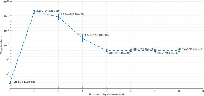
Figure 2: The average output variance of 1000 Monte Carlo simulations. The mean(std) values of $({\bf h}_{k}(\textbf{{x}}_{0})\boldsymbol{\epsilon})^{2}$, $k=1,...,8$ are indicated for each error bar. Due to taking of logarithm on negative values, the lower portion of the error bar is a mere replica of the upper portion for visualization purpose.

Remark 3: The analysis of output variance shows that the variance of estimation does not diverge for deep networks when the hidden layers are estimated using the data image (i.e., the pseudoinverse of the data matrix). This result is congruence with the observation of good generalization obtained in deep networks in the literature. Numerically, the result in Proposition 2 can be validated by a Monte Carlo simulation as follows. To keep the outputs of deeper networks within the visible changing range, an activation function of the exponential form (i.e., $e^{0.0001{\bf X}{\bf W}}$) has been adopted for each layer in this study. The weights are computed deterministically according to (34) through (37). The elements of the input matrix ${\bf X}\in\mbox{$\mathbb{R}$}^{100\times 10}$ (100 samples of 10 dimensions) are generated randomly within $[-5,+5]$. The vector $\textbf{{x}}_{0}\in\mbox{$\mathbb{R}$}^{100\times 1}$ in (51) is also generated randomly within the same range. The learning target vector ${\bf y}\in\{-1,+1\}$ contains 100 samples with half of the total samples for each category. The noise vector $\boldsymbol{\epsilon}\in\mbox{$\mathbb{R}$}^{100\times 1}$ in (51) is taken to be of one-tenth magnitude of the input elements’ range. A 1000 Monte Carlo simulations have been conducted for the random setting. Fig. 2 shows the average plot of $({\bf h}_{k}(\textbf{{x}}_{0})\boldsymbol{\epsilon})^{2}$ for the 1000 random trials over $k=1,2,\cdots,8$ which correspond to the number of layers of each network. By excluding the linear network without the exponential activation at $k=1$ (i.e., $({\bf h}_{1}(\boldsymbol{x}_{0})\boldsymbol{\epsilon})^{2}$ where $\boldsymbol{x}_{0}\in\mbox{$\mathbb{R}$}^{10\times 1}$ which has a different dimension from that of $\textbf{{x}}_{0}\in\mbox{$\mathbb{R}$}^{100\times 1}$), it can be seen that the value of the output variance $({\bf h}_{k}(\textbf{{x}}_{0})\boldsymbol{\epsilon})^{2}$ does not diverge for networks with more than two layers. This result may contribute to explaining the non-overfitting behavior of deep networks. $\square$

5 Case Studies

In this section, two sets of synthetic data with known function generators are adopted to observe the learning and representation properties of the proposed network. The first data set studies the fitting ability in terms of training data representation with respect to the scaling of the initial weights. The second data set studies the decision boundary of a learned network as well as the number of nodes needed in the hidden layer for representation.

Without loss of generality, a modified softplus function $f(x)=\log(0.8+e^{x})$ and its inverse given by $f^{-1}(x)=\log(e^{x}-0.8)$ are adopted in the learning algorithm in Corollary 1 (abbreviated as ANNnet) for all the numerical studies and experiments. The computing platform is an Intel Core i7-6500U CPU at 2.59GHz with 8GB of RAM.

5.1 A regression problem

In this example, we examine the effect of initial weight magnitudes (based on a scaling factor $c$ which is multiplied to the initial weight matrices elementwise) and the effect of network layers using a single dimensional regression function. A total of 8 training target samples $y_{i}$, $i=1,2,\cdots,8$ are generated based on the function $y=\sin(2x)/(2x)$ using $x_{i}\in\{1,2,\cdots,8\}$. Apart from this set of training samples, another 10 sets (each set containing 8 samples) of training target samples are generated by adding 20% of noisy variations with respect to the training target range. Our purpose is to observe the mapping capability of the network to learn these 11 curves with different curvatures using different $c$ settings and the number of network layers. In order to observe the fine fitting points of the network, for each curve, another set of output samples is generated using a higher resolution input $x_{j}\in\{0.90,0.91,\cdots,8.09,8.10\}$. This test set or observation set contains 721 samples.

Fig. 3(a) and (b) respectively show the fitting results of a 2-layer ANNnet (of 8-1 structure) at $c=1$ and $c=0.1$. The $c$ value is a scaling factor for each of the ${\bf R}_{2}$ to ${\bf R}_{n}$ matrices in (24)-(27). The result at $c=1$ (Fig. 3(a) and Table 1) shows a perfect fit for all the training data points but with a high testing (prediction) Sum of Squared Errors (SSE) which indicate the large difference between the output of the test samples and the underneath target (blue) curve. The fitting result shows a ‘smoother’ (with lower fluctuations) curve at $c=0.1$ than that at $c=1$. In terms of the deviation of the predicted output from the target function, the SSE for the case of $c=0.1$ shows a lower value than that of $c=1$ (see the test SSE values in Table 1). These results demonstrate an over-fitting case for Fig. 3(a) and an under-fitting case for Fig. 3(b) in terms of the training data where the SSE of training data is compromised.

The results for a 5-layer ANNnet (of 1-1-1-8-1 structure) at $c=1$ and at $c=0.1$ show a similar trend of having a ‘smoother’ fit in the lower $c$ value. However, this smoother fit with lower fluctuations does not compromise the training SSE values while maintaining a low SSE for the test data (see Table 1). This is different from that of the 2-layer case where the smoother fit compromises in fitting every data points. This fitting behavior can be observed from the almost zero training SSE values for both $c$ value settings in the 5-layer network. These results show a better generalization capability for the 5-layer network than the 2-layer network.

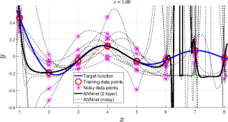
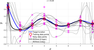
(a)	(b)
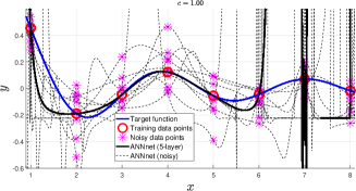
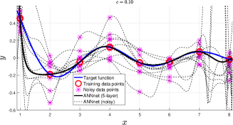
(c)	(d)

Figure 3: Learned outputs of the ANNnet at different scaling $c$ settings for 2-layer and 5-layer networks.

Table 1: Sum of Squared Errors (training/test)

Methods	$c=1$, $s=0$	$c=0.1$, $s=0$
2-layer ANNnet	1.8421$\times 10^{-19}$/1.3512$\times 10^{5}$	1.1500$\times 10^{-2}$/1.1143$\times 10^{2}$
5-layer ANNnet	9.0015$\times 10^{-13}$/1.2507$\times 10^{6}$	7.6328$\times 10^{-14}$/1.2426$\times 10^{2}$

5.2 The Spiral problem

The spiral problem is well known in studying the mapping capability of neural networks. It has been shown to be intrinsically connected to the inside-outside relations [49]. In this example, a 6-arm spiral pattern has been generated with each arm being perturbed by random noise (i.e., rotation_angle + 0.3$\times$rand). Each arm contains a total of 500 samples with half being used for training and the remaining half for test. In other words, the training set and the test set each contains 1500 samples for the 6 arms ($1500=250\times 6$). A 4-layer network of 150-250-150-6 structure has been used to learn the data using the training set. The classification accuracy performance is measured by counting the number of test samples which fall out of the decision boundary. By using the softplus8 activation function with $c=0.5$ for scaling the initial weights, an error free testing result is achieved. Fig. 4 shows the learned decision boundary with the test samples.

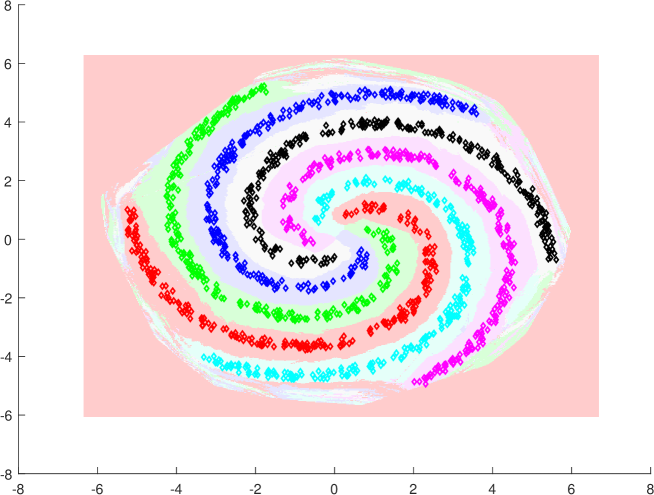
Figure 4: Testing data points and the decision boundary of a trained ANNnet.

Fig. 5 shows the Sum of Squared Errors (SSE) of training results for 10 trials using different random seeds for the weights ${\bf R}_{2},\cdots,{\bf R}_{n}$ initialization. The adopted network structure is similar to that of the above except for the number of hidden nodes $h_{3}$ which is varied from 1250 to 1600 at an interval of 50. In a nutshell, a network structure of 150-250-$h_{3}$-6 has been adopted with $h_{3}$ varies within $\{1250,1300,\cdots,1550,1600\}$ in order to observe its effect on network representation. The purpose of choosing $h_{3}$ in this range is to cover the training sample size (1500) for observing the accuracy of fit. The results in Fig. 5 show zero SSE for $h_{3}\geqslant 1500$ which reflect the representation capability of the network for the 1500 training samples.

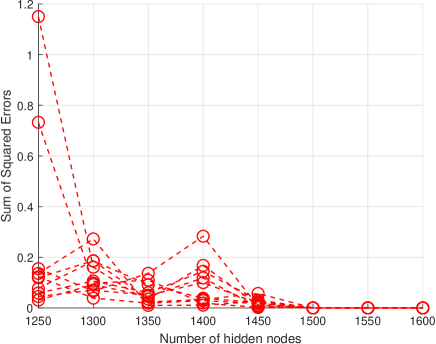
Figure 5: Variation of the training Sum of Squared Errors (SSE) over the number of hidden nodes at layer $h_{3}$ for 10 trails based on different random seeds.

Fig. 6(a) and (b) show respectively the SSEs for variation of $h_{2}$ and $h_{1}$ nodes while fixing the other two layers at 150 nodes. These results show a variation of the minimum number of hidden nodes needed for training data representation (in order to arrive at an almost zero training SSE) towards the input layer.

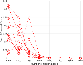
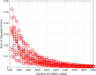
(a) Number of $h_{2}$ hidden nodes	(b) Number of $h_{1}$ hidden nodes

Figure 6: Variation of the training Sum of Squared Errors (SSE) over the number of hidden nodes ((a) at layer $h_{2}$ and (b) at layer $h_{1}$) for 10 trails based on different random seeds.

6 Experiments

In this section, the proposed learning algorithm is evaluated using real-world data sets taken from the UCI Machine Learning Repository [50]. Our goals are (i) to observe whether the gradient-free learning is numerically feasible for real-world data of small to medium size on a computer with 8 GB of RAM and without GPU? If feasible, how is the accuracy comparing with that of the conventional network learning? (ii) the computational CPU performance, (iii) Finally, the effects of network depth and sparseness are evaluated using 2-, 3- and 5-layer networks on the relatively humble computer platform.

6.1 UCI Data Sets

The UCI data sets are selected according to [51] and are summarized in Table 2 with their pattern attributes. The experimental goals (i) and (iii) are evaluated by observing the prediction accuracy of the algorithm. The accuracy is defined as the percentage of samples being classified correctly. The experimental goal (ii) is observed by recording the training CPU processing time of the compared algorithms on an Intel Core i7-6500U CPU at 2.59GHz with 8GB of RAM memory. The training CPU time is measured using the Matlab’s function cputime which corresponds to the total computational times from each of the 2 cores in the Processor. In other words, the physical time experienced is about 1/2 of this clocked cputime.

Table 2: Summary of UCI [50] data sets and chosen hidden layer sizes ($h$) based on cross-validation within the training set

		(i)	(ii)	(iii)	(iv)	2-layer		3-layer	5-layer
						( $h$ )	( $h$ )	( $h$ )	( $h$ )
	Database name	#cases	#feat	#class	#miss	FFnet	ANNnet	ANNnet	ANNnet
1.	Shuttle-l-control	279(15)	6	2	no	3	3	5	5
2.	BUPA-liver-disorder	345	6	2	no	2	500	3	2
3.	Monks-1	124(432)	6	2	no	5	1	2	2
4.	Monks-2	169(432)	6	2	no	10	200	500	80
5.	Monks-3	122(432)	6	2	no	5	1	3	5
6.	Pima-diabetes	768	8	2	no	3	2	3	10
7.	Tic-tac-toe	958	9	2	no	20	30	500	10
8.	Breast-cancer-Wiscn	683(699)	9(10)	2	16	10	3	3	3
9.	StatLog-heart	270	13	2	no	2	20	3	3
10.	Credit-app	653(690)	15	2	37	1	3	1	5
11.	Votes	435	16	2	yes	10	2	3	3
12.	Mushroom	5644(8124)	22	2	attr#11	5	80	50	10
13.	Wdbc	569	30	2	no	2	10	2	5
14.	Wpbc	194(198)	33	2	4	1	5	500	80
15.	Ionosphere	351	34	2	no	10	1	2	2
16.	Sonar	208	60	2	no	30	5	3	3
17.	Iris	150	4	3	no	20	10	10	5
18.	Balance-scale	625	4	3	no	20	50	20	5
19.	Teaching-assistant	151	5	3	no	50	500	80	80
20.	New-thyroid	215	5	3	no	5	20	10	5
21.	Abalone	4177	8	3(29)	no	50	30	20	10
22.	Contraceptive-methd	1473	9	3	no	20	50	20	3
23.	Boston-housing	506	12(13)	3(cont)	no	50	50	10	5
24.	Wine	178	13	3	no	50	30	10	5
25.	Attitude-smoking+	2855	13	3	no	1	1	1	1
26.	Waveform+	3600	21	3	no	20	5	20	5
27.	Thyroid+	7200	21	3	no	3	80	20	30
28.	StatLog-DNA+	3186	60	3	no	10	20	10	20
29.	Car	2782	6	4	no	200	500	200	80
30.	StatLog-vehicle	846	18	4	no	10	50	20	10
31.	Soybean-small	47	35	4	no	1	3	3	3
32.	Nursery	12960	8	4(5)	no	100	500	80	100
33.	StatLog-satimage+	6435	36	6	no	5	500	200	20
34.	Glass	214	9(10)	6	no	80	10	20	5
35.	Zoo	101	17(18)	7	no	20	20	50	100
36.	StatLog-image-seg	2310	19	7	no	100	500	200	–
37.	Ecoli	336	7	8	no	20	50	20	5
38.	LED-display+	6000	7	10	no	100	50	20	100
39.	Yeast	1484	8(9)	10	no	100	100	30	10
40.	Pendigit	10992	16	10	no	200	500	500	50
41.	Optdigit	5620	64	10	no	200	500	500	30
42.	Letter	20000	16	26	no	–	500	500	200

(i-iv)	:	(i) Total number of instances, i.e. examples, data points, observations (given number of instances). Note: the number of instances used is larger than the given number of instances when we expand those “don’t care” kind of attributes in some data sets; (ii) Number of features used, i.e. dimensions, attributes (total number of features given); (iii) Number of classes (assuming a discrete class variable); (iv) Missing features;
$+$	:	Accuracy measured from the given training and test set instead of 10-fold validation (for large data cases with test set containing at least 1,000 samples);
FFnet	:	The feedforwardnet from the Matlab’s toolbox using default settings;
$h$	:	The number of hidden nodes for 2layer, 3layer, and 5layer networks are set as $h$-$q$, $2h$-$h$-$q$, and $8h$-$4h$-$2h$-$h$-$q$ respectively;
Note	:	Data from the Attitudes Towards Smoking Legislation Survey - Metropolitan Toronto 1988, which was funded by NHRDP (Health and Welfare Canada), were collected by the Institute for Social Research at York University for Dr. Linda Pederson and Dr. Shelley Bull.

(i) Feasibility and prediction accuracy of two-layer networks

In this experiment, the prediction accuracy of ANNnet is recorded and compared with that of the feedforwardnet (abbreviated as FFnet) from the Matlab’s toolbox [52] based on the fully connected network structure of two-layers. The activation function adopted for ANNnet is softplus with random weights initialization, whereas FFnet adopted the default ‘tansig’ activation function (since softplus does not converge well enough in this case) with the ‘trainlm’ learning search. The test performance is evaluated based on 10 trails of 10-fold stratified cross-validation tests for each of the data set. The selection of the number of hidden nodes for each network is based on another 10-fold cross-validation within the training set. The search for the number of hidden nodes $h$ is conducted within the set $\{$1, 2, 3, 5, 10, 20, 30, 50, 80, 100, 200, 500$\}$. Table 2 summarizes the chosen hidden node sizes for the experimented networks for each data set. Apparently, there seems to have no strong correlation between the choice of hidden node sizes for the two networks of two-layer.

Fig. 7 shows the average prediction accuracy recorded from the 10 trails of stratified 10-fold cross-validation tests. The plot verifies (i) the feasibility of gradient-free computation for real-world data with none of the results running into computational ill-conditioning. Moreover, the results show a comparable average prediction accuracy for ANNnet (with grand average accuracy of 82.03% on the first 41 data sets) and FFnet (with grand average accuracy of 82.36% on the first 41 data sets) for most data sets. The result for the 42nd data set for FFnet was not available due to insufficient memory in our computing platform. As indicated by the shaded regions, these results show a significantly larger fluctuation of prediction accuracies for FFnet (where its results vary within the green region) than that of ANNnet (red region) over the 10 trials of 10-fold cross-validation tests.

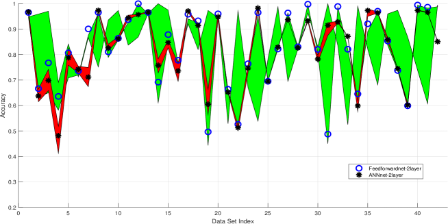
Figure 7: Prediction accuracy based on the average of 10 trials of 10-fold cross-validations. The shaded region depicts the maximum and minimum accuracy bounds and the mean accuracies for FFnet (green) and ANNnet (red) are respectively indicated by circles and asterisks.

(ii) The training CPU processing time

Fig. 8 shows the training CPU processing times (which are measured using the cputime function that accounts for per core processing time) of FFnet and ANNnet based on the same hidden node size for each data set. These results show at least an order (10 times) of speed-up for ANNnet over FFnet in terms of the training time. The maximum ratio of training time speed-up (CPU(FFnet)/CPU(ANNnet)) is $3.47\times 10^{7}$. The main reason for the speed up in training time is the gradient-free analytic training solution. Although the training time can be much faster than the conventional search mechanism, it is noted that the proposed method requires a relatively large size of RAM memory to compute the pseudoinverse of the entire data matrix.

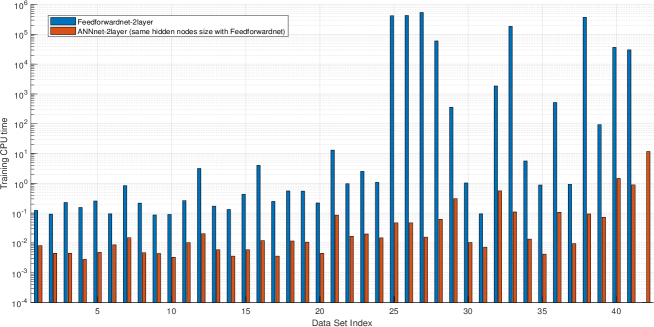
Figure 8: Comparing the training CPU time of ANNnet with that of Feedforwardnet adopting the same number of hidden nodes.

(iii) The effect of deep layers and sparseness

Effect of deep layers: Fig. 9 shows the average accuracy of ANNnet with 2-layer, 3-layer and 5 layer structures plotted respectively for each data set. The 2-layer network uses a structure of $h$-$q$ with hidden layer size $h$ and output layer size $q$. The 3-layer network uses a $2h$-$h$-$q$ structure and the 5-layer network uses a $8h$-$4h$-$2h$-$h$-$q$ structure. The size of $h$ is determined based on a cross-validation search within the training set for $h\in\{$1, 2, 3, 5, 10, 20, 30, 50, 80, 100, 200, 500$\}$. The results in Fig. 9 shows that the 5-layer ANNnet outperformed the other two networks for many data sets. The grand average results for ANNnet of 2-layer, 3-layer and 5 layer are respectively 81.75%, 81.28% and 84.13%. These results appear to support good generalization for the network of 5 layers.

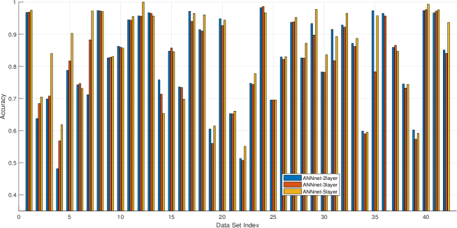
Figure 9: The effect of layers on accuracy performance.

Effects of weight scaling and sparseness: When the scaling factor, $c$, for random initialization was set at 0.1, the grand average accuracy for ANNnet was slightly improved (82.21% on the first 41 data sets according to the results in (i)) for the two-layer network. As for the sparseness setting (receptive field $r$) the gross average accuracies are observed to be 82.30% and 83.02% respectively for the fully-connected and sparsely-connected (with receptive field of $r=3$ units in the first layer) two-layer ANNnets. In other words, the fully connected network and the sparse network are with structures $h_{1}$-$h_{2}$ and $h_{1}^{r_{3}}$-$h_{2}$ respectively. For the three-layer ANNnet, the observed gross average accuracies are 81.82% and 81.93% respectively for the fully-connected ($h_{1}$-$h_{2}$-$h_{3}$) and the sparsely-connected ($h_{1}^{r_{3}}$-$h_{2}$-$h_{3}$) cases. These results (in Fig. 10) show a more significant impact of the weight scaling than the receptive field (sparseness) on the generalization performance.

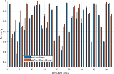
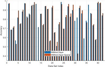
(a) Sparse 2-layer ANNnet	(b) Sparse 3-layer ANNnet

Figure 10: Comparing a non-sparse network (blue bars) with a sparse network (red bars): (a) 2-layer ANNnet, (b) 3-layer ANNnet.

6.2 Summary of Results and Discussion

Summary of Experimental Results

In summary, the three goals of the experiments have been achieved as follows:

• Based on an extensive numerical study utilizing 42 real-world data sets of small to medium sizes in terms of their dimension and sample sizes, the numerical feasibility of network learning based on the Moore-Penrose inverse is clearly verified. The structures of networks being studied included two-, three- and five-layers where few serious numerical stability issues are observed.

• The prediction accuracy of the proposed learning is observed to be comparable with that of the conventional gradient based learning. Attributed to the analytic learning formulation, the training processing time is observed to be at least 10 times faster than that of the conventional learning. For some data sets, the maximum learning speed-up can go as high as $3.47\times 10^{7}$.

• Based on the study on networks of two-, three- and five-layers, the five-layer network shows more than 2% better prediction accuracy than that of the other two networks in terms of the grand average accuracy over all data sets.

• The study shows that both the weights scaling and the sparseness of weights affect the generalization performance. This shall be a good topic for further research in the future.

Discussion and Future Works

Capitalized on the classical learning theory on Moore-Penrose inverse, an analytical learning formulation for multilayer neural networks has been proposed. Essentially, the gradient-free learning is based on the minimization approximation through the Moore-Penrose inverse projection via the column and row spaces. Based on the projection manipulation, it turns out that the solutions to the layer weights are interdependent. However, thanks to the enormous number of feasible solutions available in the network, an analytical learning can be obtained by having the weights initialized layer by layer. Though not limited to randomness, the feasibility of such a solution has been demonstrated by randomly initialized weights in experimentation. Based on these results, the following possibilities for future research are observed.

• The formulation based on the layered full matrix network structure with elementwise operated activation functions does not depart from the conventional system of linear equations. Thanks to the inherent least squares approximation property of the Moore-Penrose inverse, such a formulation allows the network solution to be written in analytical form. This treatment in the linear system form not only makes the formulation analytic and transparent but also opens up vast research possibilities towards understanding of network learning and optimization.

• An immediate possibility for such research is regarding the effect of network depth towards prediction generalization. Attributed to the layered matrix structure that hinged upon the system of linear equations, the number of possible alternative solution to the system has been shown to be exponentially increased. This opens up the vast possibilities in initializing the network weights towards good generalization.

• Other possibilities include the structural construction particularly the sparse structure and the scale of the initial weights where they are found to influence the prediction generalization in the numerical experiments.

7 Conclusion

Capitalized on the inherent property of least squares approximation offered by the Moore-Penrose inverse, a gradient-free approach for solving the learning problem of multilayer neural networks was proposed. The solution obtained from such an approach showed that network learning boiled down to solving a set of inter-dependent weight equations. By initializing the inner weight matrices either by random matrices or by the data matrix, it turned out that the interdependency of weight equations can be decoupled where an analytic learning can be achieved. Based on the analytic solution, the network representation and generalization properties with respect to the layer depth were subsequently analyzed. Our numerical experiments on a wide range of data sets of small to medium sizes not only validated the numerical feasibility, but also demonstrated the generalization capability of the proposed network solution.

References

- [1] Y. LeCun and Y. Bengio, “Convolutional networks for images, speech, and time series,” The handbook of brain theory and neural networks, pp. 255–258, 1998.
- [2] A. Krizhevsky, I. Sutskever, and G. E. Hinton, “Imagenet classification with deep convolutional neural networks,” in Proceedings of the 25th International Conference on Neural Information Processing Systems (NIPS 2012), 2012, pp. 1097–1105.
- [3] C. Szegedy, W. Liu, Y. Jia, P. Sermanet, S. Reed, D. Anguelov, D. Erhan, V. Vanhoucke, and A. Rabinovich, “Going deeper with convolutions,” in Proc. International Conference on Computer Vision and Pattern Recognition (CVPR), 2015, pp. 1–9.
- [4] K. Simonyan and A. Zisserman, “Very deep convolutional networks for large-scale image recognition,” 2014. [Online]. Available: https://arxiv.org/abs/1409.1556
- [5] K. He, X. Zhang, S. Ren, and J. Sun, “Deep residual learning for image recognition,” in Proc. International Conference on Computer Vision and Pattern Recognition (CVPR), 2016, pp. 770–778.
- [6] G. Huang, Z. Liu, L. van der Maaten, and K. Q. Weinberger, “Densely connected convolutional networks,” in Proc. International Conference on Computer Vision and Pattern Recognition (CVPR), 2017, pp. 4700–4708.
- [7] P. Baldi and K. Hornik, “Neural networks and principal component analysis: Learning from examples without local minima,” Neural Networks, vol. 2, pp. 53–58, 1989.
- [8] P. Baldi, “Linear learning: Landscapes and algorithms,” in Advances in Neural Information Processing Systems (NIPS 1988), 1988, pp. 65–72.
- [9] P. Baldi and Z. Lu, “Complex-valued autoencoders,” Neural Networks, vol. 33, pp. 136–147, 2012.
- [10] K. Kawaguchi, “Deep learning without poor local minima,” in Proceedings of the 29th International Conference on Neural Information Processing Systems (NIPS 2016), 2016, pp. 586–594.
- [11] A. Choromanska, M. Henaff, M. Mathieu, G. B. Arous, and Y. LeCun, “The loss surfaces of multilayer networks,” in Proceedings of the Eighteenth International Conference on Artificial Intelligence and Statistics, 2015, pp. 192–204.
- [12] A. Choromanska, Y. LeCun, and G. B. Arous, “Open problem: The landscape of the loss surfaces of multilayer networks,” in Proceedings of The 28th Conference on Learning Theory, 2015, pp. 1756–1760.
- [13] H. Lu and K. Kawaguchi, “Depth creates no bad local minima,” pp. 1–10, 2017. [Online]. Available: https://arxiv.org/abs/1702.08580
- [14] C. Yun, S. Sra, and A. Jadbabaie, “Global optimality conditions for deep neural networks,” in Proceedings of the 6th International Conference on Learning Representations (ICLR 2018), Vancouver, BC, Canada, 2018, pp. 1–14.
- [15] L. Dinh, R. Pascanu, S. Bengio, and Y. Bengio, “Sharp minima can generalize for deep nets,” 2017. [Online]. Available: https://arxiv.org/pdf/1703.04933.pdf
- [16] Y. N. Dauphin, R. Pascanu, C. Gulcehre, S. G. Kyunghyun Cho, and Y. Bengio, “Identifying and attacking the saddle point problemin high-dimensional non-convex optimization,” in Advances in Neural Information Processing Systems (NIPS 2014), 2014, pp. 2933–2941.
- [17] K. Chen, L. Xu, and H. Chi, “Improved learning algorithms for mixture of experts in multiclass classification,” Neural Networks, vol. 12, no. 9, pp. 1229–1252, 1999.
- [18] H. Li, Z. Xu, G. Taylor, and T. Goldstein, “Visualizing the loss landscape of neural nets,” in Proceedings of the 6th International Conference on Learning Representations (ICLR 2018), Vancouver, BC, Canada, 2018, pp. 1–17.
- [19] Q. Liao and T. Poggio, “Theory of deep learning II: Landscape of the empirical risk in deep learning,” CBMM Memo No. 066, pp. 1–45, June 2017.
- [20] S. Gunasekar, J. D. Lee, D. Soudry, and N. Srebro, “Implicit bias of gradient descent on linear convolutional networks,” in Proceedings of the 29th International Conference on Neural Information Processing Systems (NIPS 2016), 2018, pp. 1–22.
- [21] T. Poggio, Q. Liao, B. Miranda, A. Banburski, X. Boix, and J. Hidary, “Theory of deep learning IIIb: Generalization in deep networks,” CBMM Memo No. 090, pp. 1–37, June 2018.
- [22] J. Langford and R. Caruana, “(Not) Bounding the true error,” in Advances in Neural Information Processing Systems 14, T. G. Dietterich, S. Becker, and Z. Ghahramani, Eds. MIT Press, 2002, pp. 809–816. [Online]. Available: http://papers.nips.cc/paper/1968-not-bounding-the-true-error.pdf
- [23] G. K. Dziugaite and D. M. Roy, “Computing nonvacuous generalization bounds for deep (stochastic) neural networks with many more parameters than training data,” 2017. [Online]. Available: https://arxiv.org/pdf/1703.11008.pdf
- [24] B. Neyshabur, “Implicit regularization in deep learning,” Ph.D. dissertation, Toyota Technological Institute at Chicago, 2017.
- [25] B. Neyshabur, S. Bhojanapalli, and N. Srebro, “A PAC-Bayesian approach to spectrally-normalized margin bounds for neural networks,” in Proceedings of the 6th International Conference on Learning Representations (ICLR 2018), Vancouver, BC, Canada, 2018, pp. 1–9.
- [26] P. L. Bartlett, D. J. Foster, and M. Telgarsky, “Spectrally-normalized margin bounds for neural networks,” in Advances in Neural Information Processing Systems (NIPS 2017), 2017, pp. 6241–6250.
- [27] B. Neyshabur, S. Bhojanapalli, D. McAllester, and N. Srebro, “Exploring generalization in deep learning,” in Advances in Neural Information Processing Systems (NIPS 2017), 2017, pp. 5947–5956.
- [28] K. Kawaguchi, L. P. Kaelbling, and Y. Bengio, “Generalization in deep learning,” 2018. [Online]. Available: https://arxiv.org/pdf/1710.05468.pdf
- [29] R. Brunelli, “Training neural nets through stochastic minimization,” Neural Networks, vol. 7, no. 9, pp. 1405–1412, 1994.
- [30] P. Patrick van der Smagt, “Minimisation methods for training feedforward neural networks,” Neural Networks, vol. 7, no. 1, pp. 1–11, 1994.
- [31] K. Chen, “Deep and modular neural networks,” Handbook on Computational Intelligence, pp. 473–494, 2015, (Chapter 28).
- [32] K.-A. Toh, “Learning from the kernel and the range space,” in Proceedings of the 17th IEEE/ACIS International Conference on Computer and Information Science, Singapore, June 2018, pp. 417–422.
- [33] K.-A. Toh, Z. Lin, Z. Li, B. Oh, and L. Sun, “Gradient-free learning based on the kernel and the range space,” https://arxiv.org/abs/1810.11581, pp. 1–27, 27th October 2018.
- [34] S. L. Campbell and C. D. Meyer, Generalized Inverses of Linear Transformations, (SIAM edition of the work published by Dover Publications, Inc., 1991) ed. Philadelphia, USA: Society for Industrial and Applied Mathematics, 2009.
- [35] A. Albert, Regression and the Moore-Penrose Pseudoinverse. New York: Academic Press, Inc., 1972, vol. 94.
- [36] Adi Ben-Israel and Thomas N.E. Greville, Generalized Inverses: Theory and Applications, 2nd ed. New York: Springer-Verlag, 2003.
- [37] R. MacAusland, “The Moore-Penrose inverse and least squares,” April 2014, lecture notes in Advanced Topics in Linear Algebra (MATH 420). [Online]. Available: http://buzzard.ups.edu/courses/2014spring/420projects/math420-UPS-spring-2014-macausland-pseudo-inverse.pdf
- [38] R. O. Duda, P. E. Hart, and D. G. Stork, Pattern Classification, 2nd ed. New York: John Wiley & Sons, Inc, 2001.
- [39] P. J. Davis, Circulant Matrices. New York: Wiley, 1970, ISBN 0471057711.
- [40] G. H. Golub and C. F. Van Loan, Matrix Computations. Johns Hopkins, 1996, ISBN 978-0-8018-5414-9.
- [41] K.-I. Funahashi, “On the approximate realization of continuous mappings by neural networks,” Neural Networks, vol. 2, no. 3, pp. 183–192, 1989.
- [42] K. Hornik, M. Stinchcombe, and H. White, “Multi-layer feedforward networks are universal approximators,” Neural Networks, vol. 2, no. 5, pp. 359–366, 1989.
- [43] G. Cybenko, “Approximations by superpositions of a sigmoidal function,” Math. Cont. Signal & Systems, vol. 2, pp. 303–314, 1989.
- [44] R. Hecht-Nielsen, “Kolmogorov’s mapping neural network existence theorem,” in Proceedings of IEEE First International Conference on Neural Networks (ICNN), vol. III, 1987, pp. 11–14.
- [45] V. Ku̇rková, “Kolmogorov’s theorem and multilayer neural networks,” Neural Networks, vol. 5, no. 3, pp. 501–506, 1992.
- [46] M. Leshno, V. Y. Lin, A. Pinkus, and S. Schocken, “Multilayer feedforward networks with a nonpolynomial activation function can approximate any function,” Neural Networks, vol. 6, pp. 861–867, 1993.
- [47] C. Zhang, S. Bengio, M. Hardt, B. Recht, and O. Vinyals, “Understanding deep learning requires rethinking generalization,” in Proceedings of the 5th International Conference on Learning Representations (ICLR 2017), Toulon, France, 2017, pp. 1–15.
- [48] T. Hastie, R. Tibshirani, and J. Friedman, The Elements of Statistical Learning: Data Mining, Inference, and Prediction. Canada: Springer, 2001.
- [49] K. Chen and D. L. Wang, “Perceiving geometric patterns: from spirals to inside/outside relations,” IEEE Transactions on Neural Networks, vol. 12, no. 5, pp. 1084–1102, 2001.
- [50] M. Lichman, “UCI machine learning repository,” 2013. [Online]. Available: http://archive.ics.uci.edu/ml
- [51] K.-A. Toh, Q.-L. Tran, and D. Srinivasan, “Benchmarking a reduced multivariate polynomial pattern classifier,” IEEE Trans. on Pattern Analysis and Machine Intelligence, vol. 26, no. 6, pp. 740–755, 2004.
- [52] The MathWorks, “Matlab and simulink,” in [http://www.mathworks.com/], 2017.