Non-Markovian dynamics of the electronic subsystem in a laser-driven molecule: Characterization and connections with electronic-vibrational entanglement and electronic coherence

Abstract

Non-Markovian quantum evolution of the electronic subsystem in a laser-driven molecule is characterized through the appearance of negative decoherence rates in the canonical form of the electronic master equation. For a driven molecular system described in a bipartite Hilbert space $\cal{H}$$=$$\cal{H}$_el$\bigotimes$$\cal{H}$_vib of dimension $2\times N_{v}$, we derive the canonical form of the electronic master equation, deducing the canonical measures of non-Markovianity and the Bloch volume of accessible states. We find that one of the decoherence rates is always negative, accounting for the inherent non-Markovian character of the electronic evolution in the vibrational environment. Enhanced non-Markovian behavior, characterized by two negative decoherence rates, appears if there is a coupling between the electronic states $g$, $e$, such that the evolution of the electronic populations obeys $d(P_{g}P_{e})/dt>0$. Non-Markovianity of the electronic evolution is analyzed in relation to temporal behaviors of the electronic-vibrational entanglement and electronic coherence, showing that enhanced non-Markovian behavior accompanies entanglement increase. Taking as an example the coupling of two electronic states by a laser pulse in the Cs₂ molecule, we analyze non-Markovian dynamics under laser pulses of various strengths, finding that the weaker pulse stimulates the bigger amount of non-Markovianity. Our results show that increase of the electronic-vibrational entanglement over a time interval is correlated to the growth of the total amount of non-Markovianity calculated over the same interval using canonical measures, and connected with the increase of the Bloch volume. After the pulse, non-Markovian behavior is correlated to electronic coherence, such that vibrational motion in the electronic potentials which diminishes the nuclear overlap, implicitly increasing the linear entropy of entanglement, brings a memory character to dynamics.

I Introduction

Memory effects in the dynamics of open quantum systems Breuer and Petruccione (2002) have been extensively studied over the past decade, through new concepts proposed to tackle quantum non-Markovianity and examination of non-Markovian behavior in various scenarios involving open quantum systems Breuer (2012); Rivas et al. (2014); Breuer et al. (2016); de Vega and Alonso (2017). The classical definition of a Markovian process, implying a memoryless time evolution in a classic stochastic process, cannot be simply extended to the quantum regime, where the corresponding quantum probabilities have to be associated with measurement schemes. Definition of quantum Markovianity constitutes a recent research area Rivas et al. (2014); Breuer et al. (2016), and is still a debated subject Pollock et al. (2018a); Chakraborty (2018); Li et al. (2018).

We have to note the multiplicity of approaches to quantum non-Markovianity Rivas et al. (2014); Breuer et al. (2016); de Vega and Alonso (2017); Li et al. (2018): as deviation from semigroup dynamics Wolf et al. (2008), based on the backflow of information from the environment to the open system Breuer et al. (2009), as deviation from completely positive divisibility Rivas et al. (2010), based on the quantum Fisher information flow Lu et al. (2010), using entanglement-based measures Rivas et al. (2010); Fanchini et al. (2014); *debarba17 or quantum mutual-information-based measures Luo et al. (2012), related to the dynamical behavior of the volume of accessible states Lorenzo et al. (2013), and based on quantifiers of the negative rates in the canonical form of the time-local master equation Hall et al. (2014). Recent proposals use the spectral properties of dynamical maps Chruściński et al. (2017), and the process tensor framework Pollock et al. (2018a, b) to characterize non-Markovian behavior. These alternative approaches imply different non-Markovianity concepts and propose various measures or witnesses of quantum non-Markovianity. Comparative studies Addis et al. (2014); Chruściński and Maniscalco (2014); Neto et al. (2016) show them as offering different perspectives on the complex manifestation of quantum memory effects.

Non-Markovian quantum dynamics typically occurs when open quantum systems are coupled to structured or finite reservoirs, due to strong system-environment interactions, large initial system-environment correlations, or low temperature environments. In contrast to Markovian (memoryless) evolution of an open quantum system weakly coupled to a noisy environment, characterized by decoherence and dissipation, non-Markovian dynamics of an open system can lead to revivals of its characteristic quantum properties, such as quantum coherence and entanglement Breuer et al. (2016); Huelga et al. (2012); Orieux et al. (2015). Recent developments in experimental techniques allowing control and modification of the dynamical properties of various environments through quantum reservoir engineering Poyatos et al. (1996); *myatt2000 bring forward non-Markovian open quantum systems interacting with controllable environments Liu et al. (2011); Tang et al. (2012); Cosco et al. (2018). These experimental advances are motivating investigations on the role of non-Markovianity as a resource for quantum information processing Bylicka et al. (2014); Dong et al. (2018) or quantum metrology Escher et al. (2011); *chin12. Understanding memory effects in various quantum scenarios, such as non-Markovianity studies in driven open quantum systems Schmidt et al. (2015); *chen16; *poggi17; *sampaio17, contributes to the recent attempts to design non-Markovian systems which could be useful as resources in quantum technologies Liu et al. (2011); Huelga et al. (2012); Orieux et al. (2015).

Molecular physics has a long tradition in treating system-bath interactions, including non-Markovian influences of the environment Meier and Tannor (1999); *gaspard99; *kleinek04; *welack06; *roden09; *pomyalov10. Non-Markovian effects operate in various molecular processes, such as electron transfer in complex molecular systems Mangaud et al. (2017), environment-assisted quantum transport Rebentrost et al. (2009a) in molecular junctions Kilgour and Segal (2015); *sowa17, or excitonic energy transfer in photosynthetic complexes Rebentrost et al. (2009b). Possible applications of non-Markovianity include, for example, the use of certain molecular systems as quantum probes to reveal characteristic features of their environments Breuer et al. (2016); de Vega and Alonso (2017), or utilization of memory effects in the design of functional artificial biomaterials Burghardt et al. (2009).

Current efforts trying to exploit non-Markovianity as a resource for quantum control Reich et al. (2015) rely on the understanding of memory effects as related to a backflow of information from the environment to the system, capable of restoring system coherence. In this sense, recent investigations of strategies for quantum control of memory effects in molecular open-quantum systems seek to protect the central system from dissipation and decoherence by increasing non-Markovian bath response Puthumpally-Joseph et al. (2017); *puthumpal18; *mangaud18. Non-Markovianity enhancement leading to longer decoherence times of the central system could be exploited to increase the robustness of molecular alignment-orientation Puthumpally-Joseph et al. (2017); *puthumpal18; *mangaud18 or to preserve coherence of molecular qubits.

Electronic coherences play an essential role in chemical and biological processes, and their function is currently being investigated in new domains like attochemistry or quantum biology. Recent works on electron dynamics in molecules explore the mechanisms influencing electronic decoherence and the role played by nuclear motion in this process, especially in the presence of strong nonadiabatic couplings Vacher et al. (2017); *arnold18. On the other hand, understanding quantum coherence contributions to electronic energy transport in molecular aggregates and biological systems is a major goal in quantum biology Mohseni et al. (2014). Energy transport is examined using open quantum system approaches to treat electronic-vibrational dynamics in large molecules, in which an open ”system” containing relevant molecular electronic states is coupled to a bath of harmonic vibrational modes Roden et al. (2012); *rodenpre16; *rodenjcp16. Studies of non-Markovianity in photosynthetic complexes have shown a significant non-Markovian information flow between electronic and phononic degrees of freedom, which could play an important role in energy transfer, as well as correlations between non-Markovian behavior and long-lived quantum coherence Ishizaki et al. (2010); *aspuru11; *chen14; *chen15.

Approaches to quantum non-Markovianity using quantum information concepts have been recently developed in the theory of open quantum systems, bringing new frameworks for molecular processes with memory. Non-Markovianity is recognized as a highly context-dependent concept, whose understanding should not be based solely on the evolution of the system density operator; in fact, system-environment correlations are of direct relevance to grasp non-Markovianity more broadly Li et al. (2018). This is also our approach here: We will characterize non-Markovianity of the electronic subsystem in a diatomic molecule using canonical measures, and subsequently we proceed to understand the dynamic meaning of non-Markovian behavior by relating it to quantum correlations in the molecular system, namely entanglement with the vibrational environment and electronic coherence.

We consider a diatomic molecule described in a bipartite Hilbert space $\cal{H}$$=$$\cal{H}$_el$\bigotimes$$\cal{H}$_vib of the electronic and vibrational degrees of freedom, driven by a laser pulse which couples the electronic states inducing transfer of population and influencing the vibrational dynamics. We shall analyze the electronic subsystem as a driven open quantum system in the vibrational environment. Non-Markovianity of the electronic dynamics will be characterized using the approach introduced by Hall et al. in Ref. Hall et al. (2014), which employs the canonical form of the time-local master equation describing the open system dynamics to define non-Markovianity quantifiers based on the occurrence of negative decoherence rates. We derive the canonical measures of non-Markovianity for a 2-dimensional electronic subsystem of a laser-driven molecule, and connect non-Markovian behavior with temporal behaviors of electronic-vibrational entanglement (quantified using linear entropy and von Neumann entropy) and electronic coherence (measured with $l_{1}$ norm and Wigner-Yanase skew information).

The canonical measures Hall et al. (2014) provide a complete description of non-Markovianity in terms of canonical decoherence rates. Additionally, we shall also refer to the Bloch volume of accessible states as a non-Markovianity witness Lorenzo et al. (2013); Hall et al. (2014). Unlike the canonical measures, the Bloch volume is only a possible witness, and does not always detect non-Markovian behavior Hall et al. (2014); Rivas et al. (2014). Nevertheless, examination of non-Markovianity using different measures, besides being interesting in itself, will help to distinguish non-Markovianity regimes in the dynamical evolution, highlighting an ”enhanced non-Markovian behavior” which is detected by both measures.

The paper is structured as follows. Sec. II introduces the non-Markovianity approach used in this paper, based on the occurrence of negative decoherence rates in the time-local master equation. The definitions of the canonical measures of non-Markovianity Hall et al. (2014) and the Bloch volume characterization of non-Markovianity Lorenzo et al. (2013); Hall et al. (2014) are presented. Sec. III describes our model, allowing us to characterize non-Markovian dynamics of the electronic subsystem of a laser-driven molecule. We derive the canonical form of the master equation for a 2-dimensional electronic subsystem of a laser-driven molecule, and deduce the canonical non-Markovianity measures and the Bloch volume. Sec. IV contains a theoretical analysis of the relations between enhancement of non-Markovianity and dynamical behaviors of the electronic-vibrational entanglement and electronic coherence. Sec. V shows that enhanced non-Markovian behavior in the electronic evolution increases the uncertainty on the electronic energy. Sec. VI examines non-Markovian behavior of the electronic subsystem and its connections with electronic-vibrational entanglement and electronic coherence, taking as example the coupling of two electronic states in the Cs₂ molecule by laser pulses of several strengths. The time evolutions during the pulse and after pulse are simulated numerically, being analyzed using the non-Markovianity measures, the entropies of entanglement and the measures of electronic coherence. Our conclusions are exposed in Sec. VII. The paper includes an appendix which discusses the conditions determining the increase of distinguishability between two electronic states.

II Canonical form for a local-in-time master equation and negative decoherence rates

The concept of quantum Markovianity implicitly used here is related to the concept of divisibility of dynamical maps Wolf and Cirac (2008); Rivas et al. (2014); Breuer et al. (2016). We briefly recall the notion of divisibility, which is central to the definition of quantum (non)Markovianity in models using time-local master equations. Considering a dynamical map $\Lambda(t,0)$ which describes the evolution $\rho(t)$ $=\Lambda(t,0)\rho(0)$ of an open system state $\rho(t)$, $\Lambda(t,0)$ is a $t$-parametrized family of completely positive and trace preserving (CPTP) maps. $\Lambda(t,0)$ is defined to be divisible if it can be written as a composition of two trace-preserving maps, $\Lambda(t,0)=\Lambda(t,t^{\prime})\Lambda(t^{\prime},0)$, for all times $t\geq t^{\prime}\geq 0$, meaning that the two-parameter family $\Lambda(t,t^{\prime})$ has to exist for all $t,t^{\prime}$. The positivity (P) or complete positivity (CP) of $\Lambda(t,t^{\prime})$ lead to the notions of a P-divisible or CP-divisible family of dynamical maps. P divisibility and CP divisibility of a quantum process were both used to define the quantum dynamics of a process as being Markovian, and to build connections between the quantum and the classical concepts of Markovianity Rivas et al. (2014); Wißmann et al. (2015); Breuer et al. (2016). Moreover, the notion of $k$-divisibility of a dynamical map (with $1\leq k\leq n$ an integer, $n$ the dimension of the open system, $1$-divisibility corresponding to P divisibility, and $n$-divisibility corresponding to CP divisibility) was introduced to define a ”degree of non-Markovianity” of a quantum evolution Chruściński and Maniscalco (2014), as well as the notions of ”weak non-Markovianity” (for processes which are only P-divisible) and ”essential non-Markovianity” (for processes which are not even P-divisible).

A variety of theoretical and numerical methods are used to treat the dynamics of open quantum systems and to reveal the presence of memory effects Breuer and Petruccione (2002); Breuer (2012); Rivas et al. (2014); Breuer et al. (2016); de Vega and Alonso (2017), such as Nakajima-Zwanzig projection operator techniques Nakajima (1958); *zwanzig60, the time-convolutionless (TCL) projection operator technique Shibata et al. (1977); *chaturvedi79, or stochastic wave-function techniques Breuer et al. (1999); Strunz et al. (1999); Breuer (2004).

Quantum memory effects attached to an open system dynamics can be studied either using a non-local master equation with a memory kernel (obtained through the Nakajima-Zwanzig projection operator technique), or, equivalently, using the local in time equation given by the time-convolutionless (TCL) projection operator technique. Both approaches support an investigation of non-Markovian effects Breuer and Petruccione (2002); Chruściński and Kossakowski (2010). In the second approach, TCL provides a local-in-time first-order differential equation $\dot{\rho}(t)=$$\cal{L}$$(t)\rho(t)$ for the reduced density $\rho(t)$ characterizing the open system, on the condition that a certain operator inverse exists Breuer (2012); Breuer et al. (2016). For a time-local equation which does not involve a memory kernel and an integration over the past history of the system, the non-Markovian character of the dynamics appears in the explicit time-dependence of the generator $\cal{L}$$(t)$, which keeps the memory about the starting point Breuer (2004); Chruściński and Kossakowski (2010). The time-local generator $\cal{L}$$(t)$ obtained with TCL method is defined by a perturbation expansion with respect to the strength of the system-environment coupling, which does not guarantee the complete positivity of the resulting map $\Lambda(t,0)$ describing the evolution of the open system state between $0$ and $t$: $\rho(t)$ $=\Lambda(t,0)\rho(0)$ Breuer and Petruccione (2002); Breuer (2012).

If the requirements for preservation of the Hermiticity and the trace of $\rho(t)$ are imposed on the generator $\cal{L}$$(t)$ of the time-local master equation $\dot{\rho}(t)=$$\cal{L}$$(t)\rho(t)$, one obtains a general structure of the master equation (Eq. (7)), which is a generalization of the Gorini-Kossakowski-Sudarshan-Lindblad (GKSL) form for a memoryless master equation Breuer (2004, 2012); Rivas et al. (2014); Breuer et al. (2016). Moreover, the diagonalization procedure leading to this GKSL-like structure provides a unique, and then canonical form of the master equation, which can be used to characterize non-Markovianity of the time evolution  Hall et al. (2014).

The derivation of the canonical form for a general time-local master equation $\dot{\rho}(t)=$$\cal{L}$$(t)\rho(t)$ comes as a straightforward extension of the GKSL approach Gorini et al. (1976); Lindblad (1976). We shall briefly sketch the main steps, referring to Refs. Breuer and Petruccione (2002); Breuer (2012); Hall et al. (2014); Rivas et al. (2014) for a detailed demonstration.

Let us consider an open system described in a Hilbert space of finite dimension $d$. A complete set of $N:=d^{2}$ basis operators $\{G_{n}\}_{n=0}^{N-1}$ is introduced, having the properties

$$G_{0}=\hat{I}/\sqrt{d}~{};~{}G_{n}=G_{n}^{+}~{};~{}\text{Tr}[G_{m}G_{n}]=\delta_{mn},$$ (1)

with $\hat{I}$ being the identity operator. $G_{n}$ are orthonormal traceless operators (excepting $G_{0}$, for which Tr$[G_{0}]=1$). A general master equation $\dot{\rho}(t)=$$\cal{L}$$(t)\rho(t)$ can be written in the following form Breuer and Petruccione (2002); Hall et al. (2014):

$$\frac{d\rho}{dt}=-\frac{i}{\hbar}[H(t),\rho(t)]$$

$$+\sum_{i,j=1}^{N-1}D_{ij}(t)[G_{i}\rho(t)G_{j}-\frac{1}{2}\{G_{j}G_{i},\rho(t)\}],$$ (2)

with the operator $H(t)$ being Hermitian, and $D_{ij}(t)$ being the time-dependent elements of the Hermitian decoherence matrix $\mathbf{D}$. The Hermiticity property of the decoherence matrix leads to the existence of a unique canonical form of the master equation, which follows using the diagonal form of $\mathbf{D}$ Hall et al. (2014):

$$D_{ij}(t)=\sum_{k=1}^{N-1}U_{ik}(t)\gamma_{k}(t)U^{*}_{jk}(t),$$ (3)

where $\gamma_{k}(t)$ are the real eigenvalues of the decoherence matrix $\mathbf{D}$, and $U_{ik}(t)$ are the elements of the unitary matrix formed by the eigenvectors of $\mathbf{D}$, such that $\sum_{k=1}^{N-1}U_{ik}U^{*}_{jk}$$=\delta_{ij}$. Let us note that the trace of the decoherence matrix $\mathbf{D}$ equals the sum of the decoherence rates $\gamma_{k}(t)$ :

$$\text{Tr}[\mathbf{D}]=\sum_{k}\gamma_{k}.$$ (4)

If one defines the time-dependent decoherence operators $L_{k}(t)$ ($k=1,..,N-1$),

$$L_{k}(t):=\sum_{i=1}^{N-1}U_{ik}(t)G_{i},$$ (5)

which form an orthonormal basis set of traceless operators

$$\text{Tr}[L_{j}^{+}(t)L_{k}(t)]=\delta_{jk}~{};~{}\text{Tr}[L_{k}(t)]=0,$$ (6)

Eq. (2) can be written in the canonical form Hall et al. (2014):

$$\frac{d\rho}{dt}=-\frac{i}{\hbar}[H(t),\rho]$$

$$+\sum_{k=1}^{N-1}\gamma_{k}(t)[L_{k}(t)\rho L^{+}_{k}(t)-\frac{1}{2}\{L^{+}_{k}(t)L_{k}(t),\rho\}].$$ (7)

The canonical form (7) is similar to the Lindblad form of a memoryless master equation, but the Hamiltonian $H(t)$, the decoherence operators $L_{k}(t)$, and the decoherence rates $\gamma_{k}(t)$ are time-dependent. Moreover, the decoherence operators $L_{k}(t)$ correspond to a set of orthogonal decoherence channels, and the time-dependent decoherence rates $\gamma_{k}(t)$ obtained as eigenvalues of the decoherence matrix are uniquely determined and can be negative Hall et al. (2014).

Formulation of necessary and sufficient conditions under which the dynamics described in Eq. (7) is completely positive remains an open problem Breuer (2012); Breuer et al. (2016). If the rates are positive for all times, $\gamma_{k}(t)\geq 0$, the dynamics is completely positive, being in Lindblad form for each fixed $t$ Breuer (2012). However, there are cases where the rates $\gamma_{k}(t)$ may become temporarily negative without violating complete positivity Rivas et al. (2014); Breuer et al. (2016).

For a master equation in the GKSL-form (7) with time-dependent coefficients, it can be shown that the corresponding dynamical map satisfies CP-divisibility if and only if $\gamma_{k}(t)\geq 0$ Rivas et al. (2014); Breuer et al. (2016). The processes with a time-local master equation in the form (7) and with $\gamma_{k}(t)\geq 0$ were also named ”time-dependent Markovian” Wolf et al. (2008); Breuer et al. (2009) or ”time-inhomogeneous Markovian” Rivas et al. (2010). To summarize, it is accepted that generalized Markovian dynamics appears for a master equation in the quasi-GKSL-form (7) with decay rates $\gamma_{k}(t)\geq 0$ and a completely positive divisible dynamical map Rivas et al. (2014); Megier et al. (2017).

Non-Markovianity is related to the appearance of negative rates $\gamma_{k}(t)<0$ in master equations of structure (7), which leads to a violation of the divisibility property, and which was interpreted for specific systems in terms of a flow of information from the environment back to the open system Breuer et al. (2009); Chruściński and Maniscalco (2014).

It is interesting to remember the signification given to the occurrence of negative rates in models using stochastic unraveling of time-local non-Markovian master equations Breuer (2004); Breuer et al. (1999); Strunz et al. (1999). These models appeared as generalizations of the stochastic wave-function method previously applied to Markovian master equations, in order to simulate quantum master equations with negative transition rates Wiseman and Milburn (1993). In the non-Markovian quantum jumps unraveling Piilo et al. (2008), the open system dynamics is described in terms of an ensemble of state vectors whose non-Hermitian deterministic evolution is interrupted by random quantum jumps Addis et al. (2014). The time-dependent rates of the master equation are connected to the quantum jumps statistics. The method provides an interpretation of the negative decay rates occurring in non-Markovian dynamics in terms of reverse quantum jumps that restore previously lost quantum superpositions Piilo et al. (2008). The negative rates reflected in reverse quantum jumps are seen as a sign of non-Markovian memory indicating the exchange of information back and forth between the system and the reservoir Piilo et al. (2008).

Hall et al. Hall et al. (2014) have shown that for a finite-dimensional system, the criterion for non-Markovianity based on the violation of CP divisibility, proposed by Rivas et al. Rivas et al. (2010), is equivalent to the criterion based on the negativity of the decoherence rates appearing in the canonical form of the master equation.

We employ the canonical measures Hall et al. (2014) to detect and quantify non-Markovianity. Because of their sensitivity to individual canonical decoherence rates, they are able to completely detect non-Markovian behavior when several decoherence channels are present. Additionally, the Bloch volume of accessible states is also used as a non-Markovianity witness Rivas et al. (2014). The two following sections expose the definitions of the canonical measures and Bloch volume, respectively.

II.1 Negative decoherence rates and canonical measures of non-Markovianity

Since the appearance of negative decoherence rates in the canonical form (7) of the master equation is a feature of non-Markovianity, Hall et al Hall et al. (2014) define several measures of non-Markovianity as functions of the negative canonical decoherence rates $\gamma_{k}(t)$. These definitions are introduced in the following and will be employed in our analysis.

For an individual channel $k$ with decoherence rate $\gamma_{k}(t)$, non-Markovianity can be described using the function Hall et al. (2014)

$$f_{k}(t):=\text{max}[0,-\gamma_{k}(t)]=\frac{1}{2}[|\gamma_{k}(t)|-\gamma_{k}(t)],$$ (8)

which is 0 if the decoherence rate $\gamma_{k}(t)$ is positive, and $|\gamma_{k}(t)|$ if the decoherence rate is negative.

The canonical measure of non-Markovianity at time $t$ is defined as the sum of the individual channels measures:

$$f(t)=\sum_{k}f_{k}(t).$$ (9)

Hall et al. Hall et al. (2014) have shown that their canonical measure $f(t)$ coincides, up to a multiplicative factor $2/d$ depending on the dimension $d$ of the system, with the trace-norm measure of non-Markovianity $g(t)$ proposed by Rivas et al. Rivas et al. (2010): $g(t)=2d^{-1}f(t)$.

One can also define a total amount of non-Markovianity in a channel $k$ over the time interval [t,t’] Hall et al. (2014) as the integral

$$F_{k}(t,t^{\prime})=\int_{t}^{t^{\prime}}f_{k}(s)ds,$$ (10)

and a total amount of non-Markovianity over the time interval [t,t’] by

$$F(t,t^{\prime})=\sum_{k}F_{k}(t,t^{\prime})=\int_{t}^{t^{\prime}}f(s)ds.$$ (11)

Ref. Hall et al. (2014) also defines a non-Markov index $n(t)$ as the number of strictly negative decoherence rates:

$$n(t):=\#\{k:\gamma_{k}(t)<0\}.$$ (12)

The orthogonality of the decoherence channels allows the interpretation of the non-Markov index $n(t)$ as the dimension of the space of non-Markovian evolution, orthogonal to the Markovian region Hall et al. (2014).

II.2 Bloch volume characterization of non-Markovianity

Lorenzo et al. Lorenzo et al. (2013) proposed a geometrical characterization of non-Markovianity based on the increase of the volume of states dynamically accessible to the system. The proposal originates in the observation that for a dynamical map corresponding to a Markovian quantum evolution the volume of physical states decreases monotonically in time, as there is no recovery of information, energy, or coherence by the system. On the contrary, a time evolution leading to a growth in the volume of accessible states reveals physical effects associated with non-Markovianity.

Ref. Hall et al. (2014) shows that, for a $d$-dimensional quantum system which can be represented by a generalized Bloch vector of dimension $d^{2}-1$, the Bloch volume $\mathcal{V}(t)$ at time $t$ is only sensitive to the sum of the canonical decoherence rates, $\sum_{k}\gamma_{k}(t)$, as follows:

$$\mathcal{V}(t)=\mathcal{V}_{0}\exp\left[-d\int_{0}^{t}ds\sum_{k}\gamma_{k}(s)\right],$$ (13)

with $\mathcal{V}_{0}$ being the initial volume at the time $t=0$. Consequently, the Bloch volume can increase at time $t$, becoming a witness of non-Markovianity, if and only if the sum of the canonical decoherence rates is negative: $\sum_{k}\gamma_{k}(t)<0$ Hall et al. (2014). Being only sensitive to the sum of the decoherence rates, there are cases when the Bloch volume cannot witness non-Markovianity Hall et al. (2014); Rivas et al. (2014), as it will also appear in this paper.

III Non-Markovianity in the reduced time evolution of the electronic subsystem of a laser-driven molecule

We will now consider the time evolution of the electronic subsystem of a molecule driven by a laser pulse which creates entanglement between electronic and vibrational degrees of freedom. We treat the electronic subsystem as an open quantum system in the vibrational environment. A non-Markovian character of the electronic system dynamics is expected, since the vibrational environment is a dynamical one, being structured by the vibrational motion in the electronic molecular potentials coupled by the laser pulse. Therefore, the non-Markovian effects in the electronic evolution will be determined by the traits of the vibrational dynamics and of the driving field. This section exposes our model, allowing us to characterize non-Markovianity of the electronic evolution using the measures introduced in the precedent section. We begin by describing the theoretical model of a diatomic molecule driven by a coupling between electronic states, such that several electronic states could be populated. The intramolecular dynamics of such a molecule is characterized by electronic-vibrational entanglement and electronic coherence Vatasescu (2013, 2015, 2016). Subsequently, we will deduce the canonical form of the master equation for a 2-dimensional electronic subsystem, building the non-Markovianity measures from the canonical decoherence rates.

We consider a diatomic molecule described in the Born-Oppenheimer (BO) approximation Lefebvre-Brion and Field (2004), neglecting the rotational degree of freedom, such that the molecular system is described by states $|\Psi_{el,vib}(t)>$ of the Hilbert space $\cal{H}$$=$$\cal{H}$_el$\bigotimes$$\cal{H}$_vib.

We assume the molecule driven by the total Hamiltonian

$$\mathbf{\hat{H}}=\hat{H}_{mol}+\hat{W}(t),$$ (14)

where the molecular Hamiltonian $\hat{H}_{mol}=\hat{H}_{el}+\hat{T}_{R}$ is the sum of the electronic Hamiltonian $\hat{H}_{el}$ and the nuclear kinetic-energy $\hat{T}_{R}$. $\hat{W}(t)$ describes a time-dependent coupling of the electronic states of the molecule . The dynamics of the molecular system is obtained from the von Neumann equation

$$i\hbar\frac{d\hat{\rho}_{el,vib}(t)}{dt}=[\mathbf{\hat{H}},\hat{\rho}_{el,vib}(t)],$$ (15)

where $\hat{\rho}_{el,vib}(t)=|\Psi_{el,vib}(t)><\Psi_{el,vib}(t)|$ is a pure state of the bipartite system (el$\bigotimes$vib).

A detailed description of the molecular model can be found in previous papers Vatasescu (2013, 2015, 2016), where we have analyzed entanglement and coherence of pure states $|\Psi_{el,vib}(t)>$ created by laser pulses. The molecular state $|\Psi_{el,vib}(t)>$ has the form

$$|\Psi_{el,vib}(t)>=\sum_{\alpha=1}^{N_{el}}|\alpha>\bigotimes|\psi_{{}_{\alpha}}(t)>,$$ (16)

the summation being over the populated electronic channels $\alpha=\overline{1,N_{el}}$. We recall that the molecular wave function $\Psi_{el,vib}(\vec{r_{i}},R,t)$ depends on the electronic coordinates $\{\vec{r_{i}}\}$ (expressed in the molecule-fixed coordinate system), the internuclear distance $R$, and the time $t$. The electronic states $|\alpha>=\phi_{\alpha}^{el}(\vec{r_{i}};R)$ (depending parametrically on R) are orthonormal eigenstates of the electronic Hamiltonian $\hat{H}_{el}$ satisfying the clamped nuclei electronic Schrödinger equation $\hat{H}_{el}|\alpha>$$=V_{{}_{\alpha}}(R)|\alpha>$, which gives the adiabatic potential-energy surfaces $V_{{}_{\alpha}}(R)$ as eigenvalues of $\hat{H}_{el}$ Lefebvre-Brion and Field (2004). $|\psi_{{}_{\alpha}}(t)>$ designates the vibrational wave packet $\psi_{{}_{\alpha}}(R,t)$ corresponding to the electronic state $|\alpha>$.

III.1 The electronic subsystem as an open quantum system entangled with the vibrational environment

We will follow the electronic subsystem dynamics in relation to dynamical behaviors of the electronic-vibrational entanglement and electronic coherence. The reduced time evolution of the electronic subsystem is derived from the unitary dynamics (Eq. (15)) of the molecular system described by the molecular density operator $\hat{\rho}_{el,vib}=|\Psi_{el,vib}(t)><\Psi_{el,vib}(t)|$, obtained with Eq. (16) as

$$\hat{\rho}_{el,vib}(t)=\sum_{\alpha,\beta}^{N_{el}}|\alpha><\beta|\bigotimes|\psi_{\alpha}(t)><\psi_{\beta}(t)|.$$ (17)

Therefore, the reduced electronic density operator $\hat{\rho}_{el}=$Tr${}_{vib}(\hat{\rho}_{el,vib})$ is Vatasescu (2015); *vatasescu2016

$$\hat{\rho}_{el}(t)=\sum_{\alpha,\beta}^{N_{el}}|\alpha><\beta|<\psi_{\beta}(R,t)|\psi_{\alpha}(R,t)>.$$ (18)

$\hat{\rho}_{el}(t)$ describes an electronic subsystem which is entangled with the vibrational environment Vatasescu (2013). For $N_{el}$ populated states, the linear entropy $L(t)=1-\text{Tr}_{el}(\hat{\rho}^{2}_{el}(t))$ of the electronic-vibrational entanglement has the expression Vatasescu (2015); *vatasescu2016:

$$L(t)=2\sum_{\alpha,\beta,\alpha\neq\beta}^{N_{el}}[P_{{}_{\alpha}}(t)P_{{}_{\beta}}(t)-|<\psi_{\alpha}(R,t)|\psi_{\beta}(R,t)>|^{2}].$$ (19)

In Eq. (19), $P_{{}_{\alpha}}(t)$$=$$<\psi_{\alpha}(R,t)|\psi_{\alpha}(R,t)>$ is the population of the electronic state $|\alpha>$, and the total population obeys the normalization condition $\sum_{\alpha=1}^{N_{el}}P_{{}_{\alpha}}(t)=1$. The other term appearing in Eq. (19) involves the off-diagonal elements $<\alpha|\hat{\rho}_{el}(t)|\beta>$$=<\psi_{\beta}(R,t)|\psi_{\alpha}(R,t)>$, which are giving the coherence of the reduced electronic state $\hat{\rho}_{el}(t)$. Using the $l_{1}$ norm definition of coherence Baumgratz et al. (2014), one obtains as measure of the electronic coherence:

$$C_{l_{1}}(\hat{\rho}_{el})=\sum_{\alpha,\beta,\alpha\neq\beta}^{N_{el}}|<\psi_{\alpha}(R,t)|\psi_{\beta}(R,t)>|.$$ (20)

In the following we suppose an electronic subsystem of dimension dim$(\cal{H}$${}_{el})=2$, and we derive the canonical form of the master equation which describes its evolution.

III.2 The master equation for a two-dimensional driven electronic subsystem

We consider a diatomic molecule in which two electronic states $|g>,|e>$ are coupled by a laser pulse, such that a pure molecular state $|\Psi_{el,vib}(t)>$ is created:

$$|\Psi_{el,vib}(t)>=|g>\bigotimes|\psi_{g}(R,t)>+|e>\bigotimes|\psi_{e}(R,t)>.$$ (21)

The quantum dynamics of the molecular system driven by the Hamiltonian (14) is given by the time-dependent Schrödinger equation:

$$i\hbar\frac{\partial}{\partial t}|\Psi_{el,vib}(t)>=[\hat{H}_{mol}+\hat{W}(t)]|\Psi_{el,vib}(t)>.$$ (22)

Projecting Eq. (22) on the electronic states $|g>,|e>$, and taking into account the BO approximation (i.e. $<\alpha|\hat{H}_{mol}|\alpha>$$=\hat{T}_{R}+V_{{}_{\alpha}}(R)$ and $<\alpha|\hat{H}_{mol}|\beta>=0$), as well as the off-diagonal nature of the coupling (i.e. $<\alpha|\hat{W}(t)|\alpha>=0$), where $|\alpha>,|\beta>$ generically designate the electronic adiabatic states, one obtains

$$i\hbar\frac{\partial}{\partial t}\left(\begin{array}[]{c}\psi_{g}(R,t)\\ \psi_{e}(R,t)\end{array}\right)=$$ (30)

$$\left(\begin{array}[]{lc}{\hat{T}_{R}}+V_{g}(R)&W(R,t)\\ W^{*}(R,t)&{\hat{T}_{R}}+V_{e}(R)\end{array}\right)\left(\begin{array}[]{c}\psi_{g}(R,t)\\ \psi_{e}(R,t)\end{array}\right).$$

Eq. (30) describes the vibrational dynamics of the wave packets $\psi_{g,e}(R,t)$ moving in the electronic potentials $V_{g}(R)$ and $V_{e}(R)$, which are coupled by $W(R,t)$$=<g|\hat{W}(t)|e>$, depending on the internuclear distance $R$ and on the time $t$. As we have mentioned, Eq. (30) can be used to describe evolution in the case of an external driving field (we will consider a laser pulse ), as well as for an internal coupling (i.e. a radial nonadiabatic coupling between electronic states).

The matrix of the reduced electronic density $\hat{\rho}_{el}(t)$ in the electronic basis $\{|g>,|e>\}$ can be deduced from Eq. (18) as

$$(\hat{\rho}_{el}(t))_{\{g,e\}}=\left(\begin{array}[]{cc}P_{g}(t)&<\psi_{e}(t)|\psi_{g}(t)>\\ <\psi_{g}(t)|\psi_{e}(t)>&P_{e}(t)\end{array}\right),$$ (33)

(34)

where $P_{g,e}(t)$$=<\psi_{g,e}(R,t)|\psi_{g,e}(R,t)>$ are the populations of the two electronic states $g,e$, with the normalization condition $P_{g}(t)+P_{e}(t)=1$. From Eq. (34) we obtain the master equation for $\hat{\rho}_{el}(t)$, having the following local-in-time form:

$$i\hbar\frac{d\hat{\rho}_{el}}{dt}=A(t)|g><g|-A(t)|e><e|$$

$$+B(t)|g><e|-B^{*}(t)|e><g|.$$ (35)

$A(t)$ and $B(t)$ are the complex time-dependent functions

$$A(t)=i\hbar\frac{dP_{g}}{dt}=-i\hbar\frac{dP_{e}}{dt},$$ (36)

$$B(t)=i\hbar\frac{d<\psi_{e}|\psi_{g}>}{dt},$$ (37)

which are determined by the time evolution of the vibrational wave packets $|\psi_{g}(R,t)>$ and $|\psi_{e}(R,t)>$, directed by Eq. (30).

The next section shows the derivation of the canonical form for Eq. (35).

III.3 Canonical form of the master equation for the two-dimensional electronic subsystem of a molecule driven by a laser pulse

We shall derive here the canonical form of the master equation for the 2-dimensional electronic subsystem $\hat{\rho}_{el}(t)$. The master equation (35) wil be used to deduce both (2) and (7) forms, in order to obtain the decoherence matrix $\mathbf{D}$ and the decoherence rates $\gamma_{k}(t)$.

As dim($\cal{H}$_el)$=2$, the orthornormal basis $\{G_{i}\}_{i=0}^{3}$ can be chosen as $\{\hat{I}/\sqrt{2},\sigma_{i}/\sqrt{2}\}$, with $\{\sigma_{i}\}_{i=1,2,3}$ being the Pauli operators: $\sigma_{1}$$=|e><g|+|g><e|$, $\sigma_{2}$$=-i|e><g|+i|g><e|$, and $\sigma_{3}$$=|e><e|-|g><g|$. We also use the operators $\sigma_{+}=|e><g|$$=1/2(\sigma_{1}+i\sigma_{2})$ and $\sigma_{-}=|g><e|$$=1/2(\sigma_{1}-i\sigma_{2})$, leading to $|g><g|=\sigma_{-}\sigma_{+}$ and $|e><e|=\sigma_{+}\sigma_{-}$. As a first step, Eq. (35) can be written as

$$i\hbar\frac{d\hat{\rho}_{el}}{dt}=\frac{A(t)}{P_{e}}\sigma_{-}\hat{\rho}_{el}\sigma_{+}-\frac{A(t)}{P_{g}}\sigma_{+}\hat{\rho}_{el}\sigma_{-}$$

$$+\frac{B(t)}{<\psi_{g}|\psi_{e}>}\sigma_{-}\hat{\rho}_{el}\sigma_{-}-\frac{B^{*}(t)}{<\psi_{e}|\psi_{g}>}\sigma_{+}\hat{\rho}_{el}\sigma_{+},$$ (38)

giving

$$\frac{d\hat{\rho}_{el}}{dt}=\sum_{i,j=1,2}d_{ij}(t)\sigma_{i}\hat{\rho}_{el}\sigma_{j}.$$ (39)

The form (39) can be completed in order to sort out an equation having the structure of Eq. (2) which provides the decoherence matrix. We then obtain

$$\frac{d\hat{\rho}_{el}}{dt}=-\frac{i}{\hbar}[H(t),\hat{\rho}_{el}(t)]$$

$$+\sum_{i,j=1}^{3}d_{ij}(t)[\sigma_{i}\hat{\rho}_{el}(t)\sigma_{j}-\frac{1}{2}\{\sigma_{j}\sigma_{i},\hat{\rho}_{el}(t)\}].$$ (40)

In Eq. (40), the Hermitian operator $H(t)$ has the following matrix in the electronic basis $\{|g>,|e>\}$:

$$(H(t))_{\{g,e\}}=$$

$$-\left(\begin{array}[]{cc}P_{g}\frac{Re(<\psi_{g}|W|\psi_{e}>)}{|<\psi_{g}|\psi_{e}>|^{2}}&\frac{<\psi_{g}|W|\psi_{e}>}{<\psi_{g}|\psi_{e}>}\\ \\ \frac{<\psi_{e}|W^{*}|\psi_{g}>}{<\psi_{e}|\psi_{g}>}&P_{e}\frac{Re(<\psi_{g}|W|\psi_{e}>)}{|<\psi_{g}|\psi_{e}>|^{2}}\end{array}\right),$$ (44)

and the matrix $d_{ij}(t)$ has the form

$$(d_{ij}(t))=\left(\begin{array}[]{ccc}d_{11}(t)&d_{12}(t)&0\\ d_{21}(t)&d_{22}(t)&0\\ 0&0&d_{33}(t)\end{array}\right).$$ (48)

The elements $D_{ij}(t)=2d_{ij}(t)$ of the Hermitian decoherence matrix $\mathbf{D}$ are the following:

$$D_{11}(t)=\frac{1}{2i\hbar}\left[\frac{A(t)}{P_{e}}-\frac{A(t)}{P_{g}}+\frac{B(t)}{<\psi_{g}|\psi_{e}>}-\frac{B^{*}(t)}{<\psi_{e}|\psi_{g}>}\right],$$

(49)

$$D_{12}(t)=\frac{1}{2\hbar}\left[\frac{A(t)}{P_{e}}+\frac{A(t)}{P_{g}}-\frac{B(t)}{<\psi_{g}|\psi_{e}>}-\frac{B^{*}(t)}{<\psi_{e}|\psi_{g}>}\right],$$

(50)

$$D_{21}(t)=D^{*}_{12}(t),$$

(51)

$$D_{22}(t)=\frac{1}{2i\hbar}\left[\frac{A(t)}{P_{e}}-\frac{A(t)}{P_{g}}-\frac{B(t)}{<\psi_{g}|\psi_{e}>}+\frac{B^{*}(t)}{<\psi_{e}|\psi_{g}>}\right],$$

(52)

$$D_{33}(t)=-i\frac{A(t)}{2\hbar}(P_{g}-P_{e})\left[\frac{1}{|<\psi_{g}|\psi_{e}>|^{2}}-\frac{1}{P_{g}P_{e}}\right],$$

(53)

$$D_{13}=D^{*}_{31}=0~{},~{}D_{23}=D^{*}_{32}=0,$$

(54)

with $A(t)$ and $B(t)$ given by Eqs. (36) and (37). Let us remark that the elements of the decoherence matrix are finite as long as $P_{g},P_{e}\neq 0$, and $<\psi_{g}|\psi_{e}>\neq 0$. These conditions are equally required in order to obtain finite values for the canonical decoherence rates, and in the following we will suppose them fulfilled.

The canonical decoherence rates $\{\gamma_{i}(t)\}_{i=1,2,3}$, obtained as eigenvalues of the decoherence matrix with elements $D_{ij}(t)$, are

$$\gamma_{1,2}(t)=\frac{1}{2P_{g}P_{e}}\frac{dP_{g}}{dt}(P_{g}-P_{e})$$

$$\pm\sqrt{\left(\frac{1}{2P_{g}P_{e}}\frac{dP_{g}}{dt}\right)^{2}+\frac{1}{|<\psi_{g}|\psi_{e}>|^{2}}\left|\frac{d<\psi_{g}|\psi_{e}>}{dt}\right|^{2}},$$

(55)

$$\gamma_{3}(t)=\frac{1}{2}\frac{dP_{g}}{dt}(P_{g}-P_{e})\left[\frac{1}{|<\psi_{g}|\psi_{e}>|^{2}}-\frac{1}{P_{g}P_{e}}\right].$$

(56)

The canonical form of the master equation appears through the diagonalization of the decoherence matrix (see Eq. (3)). We deduce the unitary matrix $(U)$ formed by the eigenvectors of the decoherence matrix $(D_{ij})$ as being

$$(U)=\left(\begin{array}[]{ccc}n_{1}&n_{2}&0\\ \\ n_{1}\frac{\gamma_{1}-D_{11}}{D_{12}}&n_{2}\frac{\gamma_{2}-D_{11}}{D_{12}}&0\\ \\ 0&0&1\end{array}\right),$$ (62)

with $\gamma_{1,2}$ being the decoherence rates given in Eq. (55) and $D_{11}$, $D_{12}$, $D_{22}$ being the elements of the decoherence matrix shown in Eqs. (49 - 52). $n_{1}$ and $n_{2}$ are real normalization factors (with $n_{1}^{2}+n_{2}^{2}=1$) given by the expressions:

$$n_{1}^{2}=\frac{\gamma_{1}-D_{22}}{\gamma_{1}-\gamma_{2}}~{};~{}n_{2}^{2}=\frac{D_{22}-\gamma_{2}}{\gamma_{1}-\gamma_{2}}.$$ (63)

The time dependent decoherence operators $\{L_{i}(t)\}_{i=1,2,3}$, corresponding to orthogonal decoherence channels are obtained using Eq. (5) as

$$L_{1}(t)=\frac{n_{1}}{\sqrt{2}}(\sigma_{1}+\frac{\gamma_{1}-D_{11}}{D_{12}}\sigma_{2}),$$ (64)

$$L_{2}(t)=\frac{n_{2}}{\sqrt{2}}(\sigma_{1}+\frac{\gamma_{2}-D_{11}}{D_{12}}\sigma_{2}),$$ (65)

$$L_{3}(t)=\frac{1}{\sqrt{2}}\sigma_{3}.$$ (66)

Finally, we obtain the canonical form for the master equation of the reduced electronic density operator $\hat{\rho}_{el}(t)$ (34):

$$\frac{d\hat{\rho}_{el}}{dt}=-\frac{i}{\hbar}[H(t),\hat{\rho}_{el}(t)]$$

$$+\sum_{i=1}^{3}\gamma_{i}(t)[L_{i}(t)\hat{\rho}_{el}L^{+}_{i}(t)-\frac{1}{2}\{L^{+}_{i}(t)L_{i}(t),\hat{\rho}_{el}\}],$$ (67)

with the operator $H(t)$ having the matrix (44), the decoherence rates $\{\gamma_{i}(t)\}_{i=1,2,3}$ given in Eqs. (55, 56), and the decoherence operators $\{L_{i}(t)\}_{i=1,2,3}$ determined by Eqs. (64-66).

The sum of the canonical decoherence rates is the trace of the decoherence matrix given by Eqs. (49 - 53):

$$\sum_{i}\gamma_{i}(t)=\text{Tr}[\mathbf{D}(t)]$$

$$=\frac{1}{2}\frac{dP_{g}}{dt}(P_{g}-P_{e})\left[\frac{1}{P_{g}P_{e}}+\frac{1}{|<\psi_{g}|\psi_{e}>|^{2}}\right],$$ (68)

becoming zero at instants $t$ for which $dP_{g}/dt=0$ or $P_{g}(t)=P_{e}(t)$.

The Bloch volume of the accessible states, obtained with Eq. (13), is

$$\mathcal{V}(t)=\mathcal{V}(t_{0})\exp\left[-2\int_{t_{0}}^{t}ds\sum_{i}\gamma_{i}(s)\right].$$ (69)

As already discussed, if the sum $\sum_{i}\gamma_{i}(t)$ of the canonical decoherence rates is negative, the Bloch volume of the accessible states increases, witnessing non-Markovianity. Therefore, a first indication on the non-Markovian behavior is given by Eq. (68) which shows that a growth of the Bloch volume, $\mathcal{V}(t)>\mathcal{V}(t_{0})$, appears if $\frac{dP_{g}}{dt}(P_{g}-P_{e})<0$.

The normalization condition $P_{g}(t)+P_{e}(t)=1$ implies

$$\frac{dP_{g}}{dt}(P_{g}-P_{e})=-\frac{d}{dt}(P_{g}P_{e}).$$ (70)

Therefore, the condition to have $\sum_{i}\gamma_{i}(t)<0$, leading to a growth of the Bloch volume, can also be expressed as $\frac{d}{dt}(P_{g}P_{e})>0$.

III.4 Decoherence rates and canonical measures of non-Markovianity for the electronic system

Let us analyze the signs of the decoherence rates $\gamma_{i}(t)$ given by Eqs. (55,56). Since $P_{g}P_{e}$ $\geq$ $|<\psi_{g}|\psi_{e}>|^{2}$, and with Eq. (70), it appears that the sign of $\gamma_{3}(t)$ depends on the time evolution of the electronic populations $P_{g}(t),P_{e}(t)$ as follows:

$$\text{sgn}[\gamma_{3}(t)]=\text{sgn}\left[\frac{dP_{g}}{dt}(P_{g}-P_{e})\right]=-\text{sgn}\left[\frac{d}{dt}(P_{g}P_{e})\right].$$

(71)

On the other hand, Eq. (55) can be written as

$$\gamma_{1,2}(t)=\frac{1}{2P_{g}P_{e}}\left|\frac{dP_{g}}{dt}\right|$$

$$\times\left\{\text{sgn}\left[\frac{dP_{g}}{dt}(P_{g}-P_{e})\right]|P_{g}-P_{e}|\pm\sqrt{1+r^{2}(t)}\right\},$$

(72)

with

$$r^{2}(t)=\frac{4P^{2}_{g}P^{2}_{e}}{(dP_{g}/dt)^{2}}\frac{|d<\psi_{g}|\psi_{e}>/dt|^{2}}{|<\psi_{g}|\psi_{e}>|^{2}}.$$ (73)

Taking into account that $0$ $\leq$ $|P_{g}-P_{e}|$ $\leq$ $1$, it becomes obvious that $\gamma_{1}(t)$ is always positive, and $\gamma_{2}(t)$ is always negative:

$$\gamma_{1}(t)>0~{};\gamma_{2}(t)<0.$$ (74)

Consequently, we will distinguish four cases:

(i) If $\frac{dP_{g}}{dt}(P_{g}-P_{e})$ $>0$, or equivalently, $\frac{d}{dt}(P_{g}P_{e})<0$, there is one negative decoherence rate, $\gamma_{2}(t)<0$, and the non-Markov index defined by Eq. (12) is $n(t)=1$. Eq. (68) shows that the sum of the decoherence rates is positive, $\sum_{i}\gamma_{i}(t)>0$, leading to a diminution of the Bloch volume.

The non-Markovianity measure obtained with Eqs. (8,9) is $f(t)=f_{2}(t)$$=|\gamma_{2}(t)|$. Using Eq. (72) we find

$$f(t)=\frac{1}{2P_{g}P_{e}}\left|\frac{dP_{g}}{dt}\right|\left[\sqrt{1+r^{2}(t)}-|P_{g}-P_{e}|\right].$$ (75)

(ii) If $\frac{dP_{g}}{dt}(P_{g}-P_{e})$ $<0$, or equivalently, $\frac{d}{dt}(P_{g}P_{e})>0$, there are two negative decoherence rates, $\gamma_{2}(t)<0$ and $\gamma_{3}(t)<0$. The dimension of the space of non-Markovian evolution, given by the non-Markov index Hall et al. (2014), becomes $n(t)=2$. The non-Markovianity measure is obtained from the negative decoherence rates using Eqs. (8) and (9), as $f(t)=f_{2}(t)+f_{3}(t)$$=|\gamma_{2}(t)|+|\gamma_{3}(t)|$. Using Eqs. (72,56) we find

$$f(t)=\frac{1}{2P_{g}P_{e}}\left|\frac{dP_{g}}{dt}\right|\left[|P_{g}-P_{e}|+\sqrt{1+r^{2}(t)}\right]$$

$$+\frac{1}{P_{g}P_{e}}\frac{d(P_{g}P_{e})}{dt}\frac{L(t)}{[C_{l_{1}}(\hat{\rho}_{el})]^{2}}.$$ (76)

In Eq. (76), $L(t)$ and $C_{l_{1}}(\hat{\rho}_{el})$ are the linear entropy of the electronic-vibrational entanglement and the electronic coherence, respectively, whose expressions can be derived from Eqs. (19,20) for $N_{el}=2$.

Moreover, the sum of the decoherence rates is negative, $\sum_{i}\gamma_{i}(t)<0$, which means that the Bloch volume of the dynamically accessible states increases (Eq. 13), witnessing non-Markovianity. We distinguish this case as indicating enhancement of non-Markovianity.

(iii) If $P_{g}(t)=P_{e}(t)$, the decoherence rates are $\gamma_{3}(t)=0$, and $\gamma_{2}(t)=-\gamma_{1}(t)$. The sum of the decoherence rates becomes zero, $\sum_{i}\gamma_{i}(t)=0$. Using Eq. (72), the non-Markovianity measure $f(t)=|\gamma_{2}(t)|$ becomes

$$f(t)=\frac{1}{2P_{g}P_{e}}\left|\frac{dP_{g}}{dt}\right|\sqrt{1+r^{2}(t)}.$$ (77)

(iv) If $\frac{dP_{g}}{dt}=0$. This condition corresponds to extrema in the evolution of the electronic populations during the pulse, or to constant populations after pulse. The decoherence rates become $\gamma_{3}(t)=0$, and $\gamma_{2}(t)=-\gamma_{1}(t)$, with $\sum_{i}\gamma_{i}(t)=0$. Eq. (55) gives

$$\gamma_{1,2}(t)=\pm\frac{1}{|<\psi_{g}|\psi_{e}>|}\left|\frac{d<\psi_{g}|\psi_{e}>}{dt}\right|,$$ (78)

and $f(t)=$$|\gamma_{2}(t)|$.

Let us consider the case of a molecule with constant populations in the electronic states $g,e$ (it can be a molecule after the action of a laser pulse): $\frac{dP_{g}}{dt}=0$ for all $t$. Therefore, the Bloch volume of the dynamically accessible states remains constant, $\mathcal{V}(t)$$=\mathcal{V}_{0}$. For $W(R,t)=0$, Eqs. (78) and (30) give an alternative form of the decoherence rates as

$$\gamma_{1,2}(t)=\pm\frac{1}{\hbar}\frac{|<\psi_{g}|V_{e}(R)-V_{g}(R)|\psi_{e}>|}{|<\psi_{g}|\psi_{e}>|}.$$ (79)

Writing the complex overlap of the vibrational packets as $<\psi_{g}|\psi_{e}>$$=|<\psi_{g}|\psi_{e}>|$ exp($i\alpha(t)$), with $\alpha(t)$ a real function, the non-Markovianity measure $f(t)=$$|\gamma_{2}(t)|$ obtained using Eq. (78) becomes

$$f(t)=\sqrt{\left(\frac{1}{|<\psi_{g}|\psi_{e}>|}\frac{d|<\psi_{g}|\psi_{e}>|}{dt}\right)^{2}+\left(\frac{d\alpha}{dt}\right)^{2}}.$$ (80)

Eq. (80) is useful for understanding the relation between $f(t)$ and the electronic coherence $|<\psi_{g}|\psi_{e}>|$. It appears that if at an instant $t_{m}$ one has ($\frac{d|<\psi_{g}|\psi_{e}>|}{dt})_{t_{m}}=0$ (an extremum in the time evolution of the coherence), but $|<\psi_{g}|\psi_{e}>|_{t_{m}}\neq 0$, one obtains a minimum of the function $f(t)$, which becomes $f(t_{m})=|\frac{d\alpha}{dt}|_{t_{m}}$. On the contrary, at an instant $t_{M}$ for which $|<\psi_{g}|\psi_{e}>|_{t_{M}}\to 0$ (which obviously represents a minimum in the time evolution of the coherence, and therefore ($\frac{d|<\psi_{g}|\psi_{e}>|}{dt})_{t_{M}}=0$), the function $f(t)$ has a maximum, becoming $f(t_{M})$$=\sqrt{1+\left(\frac{d\alpha}{dt}\right)_{t_{M}}^{2}}$. Eq. (80) shows that in a molecule with constant electronic populations, the non-Markovianity measure $f(t)$ can be seen as a measure of the temporal behavior of the electronic coherence, having minima when the electronic coherence has maxima, and attaining maximum values whenever the overlap of the vibrational packets tends to zero, $|<\psi_{g}|\psi_{e}>|\to 0$. At the same time, as we have shown previously Vatasescu (2015), if the electronic populations are constant, the time variations of the coherence $|<\psi_{g}|\psi_{e}>|$ completely determine the temporal evolution of the linear entropy of entanglement $L(t)$ (see Eq. (82)), which becomes maximum when coherence attains a minimum. Therefore, the maxima of the non-Markovianity measure $f(t)$ correspond to maxima of the electronic-vibrational entanglement measured by the linear entropy.

These results make explicit the fundamental non-Markovian character of the electronic subsystem evolution. Indeed, we have shown that one of the decoherence rates is always negative: $\gamma_{2}(t)<0$. Besides this inherent non-Markovianity, the character of the electronic evolution becomes strongly non-Markovian under the condition $(P_{g}-P_{e})$$dP_{g}/dt$ $<0$ i.e. $d(P_{g}P_{e})/dt>0$, which supposes an exchange of population between the electronic channels. In the following, $d(P_{g}P_{e})/dt$ will be called the non-Markovianity factor.

The condition $(P_{g}-P_{e})$$dP_{g}/dt$ $<0$ implies $\text{sgn}(dP_{g}/dt)$ $=-\text{sgn}[P_{g}(t)-P_{e}(t)]$. Therefore, it appears that the non-Markovian character of the dynamics is strengthened when the transfer of population between the two electronic channels is such as the larger population decreases (i.e., the smaller electronic population increases). This condition, describing an evolution oriented to the equalization of the electronic populations, is in fact a condition indicating the increase of the electronic-vibrational entanglement, which becomes maximum when the electronic populations are equal Vatasescu (2013). This observation will be developed in the following sections.

IV Connecting non-Markovianity of the electronic evolution with electronic-vibrational entanglement and electronic coherence

We will now analyze enhancement of non-Markovianity, determined by the condition $d(P_{g}P_{e})/dt>0$, in relation to the evolutions of the electronic-vibrational entanglement and the electronic coherence. The key observation is that the quantity $P_{g}(t)P_{e}(t)$ is connected to measures of entanglement and coherence in the molecular system.

The electronic-vibrational entanglement in the bipartite molecular state $|\Psi_{el,vib}(t)>$ given by Eq. (21) can be analyzed using the von Neumann entropy $S_{vN}(\hat{\rho}_{el}(t))$ or the linear entropy $L(t)$ of the reduced density operator $\hat{\rho}_{el}$. In previous works Vatasescu (2013, 2015) we have investigated the results given by these two entanglement measures. Both of them depend on the temporal behavior of the electronic populations, but only $L(t)$ depends on the electronic coherence. The von Neumann entropy of the electronic-vibrational entanglement has the following expression Vatasescu (2013):

$$S_{vN}(\hat{\rho}_{el}(t))=-P_{g}(t)\log_{2}P_{g}(t)-P_{e}(t)\log_{2}P_{e}(t).$$ (81)

For $N_{el}=2$, the linear entropy $L(t)=1-\text{Tr}(\hat{\rho}^{2}_{el}(t))$ obtained with Eq. (19) becomes

$$L(t)=2P_{g}(t)P_{e}(t)-2|<\psi_{g}(R,t)|\psi_{e}(R,t)>|^{2},$$ (82)

and, with Eq. (20), the $l_{1}$ norm measure of the electronic coherence is

$$C_{l_{1}}(\hat{\rho}_{el})=2|<\psi_{g}(R,t)|\psi_{e}(R,t)>|.$$ (83)

Therefore, Eq. (82) can be read as a relation between the phenomena of electronic-vibrational entanglement, non-Markovianity of the electronic evolution, and electronic coherence. Indeed, Eqs. (82) and  (83) lead to

$$\frac{d}{dt}[P_{g}(t)P_{e}(t)]=\frac{1}{2}\frac{dL}{dt}+\frac{1}{2}C_{l_{1}}(\hat{\rho}_{el})\frac{dC_{l_{1}}(\hat{\rho}_{el})}{dt}.$$ (84)

In the following, Eq. (84) will be used to explore the relations between enhancement of non-Markovianity ($d(P_{g}P_{e})/dt>0$), increase of entanglement ($dL/dt>0$), and increase of the electronic coherence ($dC_{l_{1}}(\hat{\rho}_{el})/dt>0$).

Expressions of the decoherence rates as functions of $L(t)$ and $C_{l_{1}}(t)$ can be given. Using Eq. (68), the sum of the decoherence rates becomes

$$\sum_{i}\gamma_{i}(t)=-\frac{d[\ln(P_{g}P_{e})]}{dt}\frac{L(t)+[C_{l_{1}}(\hat{\rho}_{el})]^{2}}{[C_{l_{1}}(\hat{\rho}_{el})]^{2}},$$ (85)

and, with Eq. (56), $\gamma_{3}(t)$ can be written

$$\gamma_{3}(t)=-\frac{d[\ln(P_{g}P_{e})]}{dt}\frac{L(t)}{[C_{l_{1}}(\hat{\rho}_{el})]^{2}}.$$ (86)

Table 1: Connections between the time behavior of the electronic-vibrational entanglement ($dL/dt$), the enhancement of non-Markovianity in the evolution of the electronic subsystem ($d(P_{g}P_{e})/dt>0$), and behaviors of speakable and unspeakable Marvian and Spekkens (2016) electronic coherences, measured by $l_{1}$ norm $C_{l_{1}}(t)$ and skew information ${\cal I_{S}}(t)$, respectively.

	$\frac{dL}{dt}$	$\frac{d(P_{g}P_{e})}{dt}$		$\frac{dC_{l_{1}}}{dt}$			$\frac{\partial{\cal I_{S}}}{\partial t}$
(1)	$>0$	$<0$	$\Longrightarrow$	$<0$			$<0$
(2)	$>0$	$>0$	$\Longrightarrow$	$>0$, if			$>0$, if
				$\frac{d(P_{g}P_{e})}{dt}>\frac{1}{2}\frac{dL}{dt}$			$\frac{1}{2\sqrt{2L}(1+\sqrt{2L})}\frac{dL}{dt}<\frac{1}{\sqrt{2L}+L+2P_{g}P_{e}}\frac{d(P_{g}P_{e})}{dt}<\frac{1}{C_{l_{1}}}\frac{dC_{l_{1}}}{dt}$
							$<0$, if
							$\frac{1}{2\sqrt{2L}(1+\sqrt{2L})}\frac{dL}{dt}>\frac{1}{\sqrt{2L}+L+2P_{g}P_{e}}\frac{d(P_{g}P_{e})}{dt}>\frac{1}{C_{l_{1}}}\frac{dC_{l_{1}}}{dt}$
				$<0$, if			$<0$
				$\frac{d(P_{g}P_{e})}{dt}<\frac{1}{2}\frac{dL}{dt}$
(3)	$<0$	$>0$	$\Longrightarrow$	$>0$			$>0$
(4)	$<0$	$<0$	$\Longrightarrow$	$<0$, if			$>0$, if
				$-\frac{1}{2}\frac{dL}{dt}<-\frac{d(P_{g}P_{e})}{dt}$			$-\frac{1}{2\sqrt{2L}(1+\sqrt{2L})}\frac{dL}{dt}>-\frac{1}{\sqrt{2L}+L+2P_{g}P_{e}}\frac{d(P_{g}P_{e})}{dt}>-\frac{1}{C_{l_{1}}}\frac{dC_{l_{1}}}{dt}$
							$<0$, if
							$-\frac{1}{2\sqrt{2L}(1+\sqrt{2L})}\frac{dL}{dt}<-\frac{1}{\sqrt{2L}+L+2P_{g}P_{e}}\frac{d(P_{g}P_{e})}{dt}<-\frac{1}{C_{l_{1}}}\frac{dC_{l_{1}}}{dt}$
				$>0$, if			$>0$
				$-\frac{1}{2}\frac{dL}{dt}>-\frac{d(P_{g}P_{e})}{dt}$

Besides the $l_{1}$ norm measure of the electronic coherence, $C_{l_{1}}(\hat{\rho}_{el})$, we shall use the Wigner-Yanase skew information ${\cal I_{S}}(\hat{\rho}_{el},\hat{H}_{el})$$=-\frac{1}{2}\text{Tr}_{el}[\sqrt{\hat{\rho}_{el}},\hat{H}_{el}]^{2}$ for the electronic state $\hat{\rho}_{el}$, with respect to the electronic Hamiltonian $\hat{H}_{el}$, to additionally characterize electronic subsystem coherence Vatasescu (2015); *vatasescu2016. The skew information ${\cal I_{S}}$ is a measure of coherence as asymmetry relative to a group of translations Marvian and Spekkens (2016); Marvian et al. (2016); Streltsov et al. (2017), quantifying the coherence of a state with respect to a certain Hamiltonian eigenbasis. This notion of coherence was termed unspeakable Marvian and Spekkens (2016), to show its structural relation to the eigenvalues of the observable which defines the basis relative to which coherence is defined . It is a notion of coherence closely related to the context of quantum speed limits Marvian et al. (2016); Streltsov et al. (2017). In particular, ${\cal I_{S}}(\hat{\rho}_{el},\hat{H}_{el})$ characterizes the coherence of the reduced electronic state $\hat{\rho}_{el}$ relative to the eigenbasis $\{|g>,|e>\}$ of the electronic Hamiltonian $\hat{H}_{el}$, whose eigenvalues are the electronic potentials $V_{g}(R),V_{e}(R)$. The skew information ${\cal I_{S}}(\hat{\rho}_{el},\hat{H}_{el})$ has the following expression Vatasescu (2015); *vatasescu2016:

$${\cal I_{S}}(\hat{\rho}_{el},\hat{H}_{el})=[V_{g}(R)-V_{e}(R)]^{2}\frac{|<\psi_{g}(R,t)|\psi_{e}(R,t)>|^{2}}{1+\sqrt{2L(t)}}.$$

(87)

${\cal I_{S}}(\hat{\rho}_{el},\hat{H}_{el})$$={\cal I_{S}}(R,t)$ appears as a product between a function of the internuclear distance $R$ (depending on the electronic potentials difference at given $R$) and a function of time $t$, a factorization which reflects the BO approximation. It can be said that ${\cal I_{S}}(R,t)$ is a measure of the unspeakable electronic coherence which characterizes the reduced electronic state $\hat{\rho}_{el}$ at a given internuclear distance $R$. Let us observe that the time behavior of ${\cal I_{S}}$ is determined by the time evolutions of the electronic coherence $C_{l_{1}}(t)$ and the linear entropy of entanglement $L(t)$. Our aim is to investigate non-Markovian behavior in relation to various quantum correlations in the molecular system, and we find it useful to also examine this measure of correlations, which combines coherence and entanglement.

Eqs. (87) and  (83) determine the relation between the time variations of the electronic coherences ${\cal I_{S}}(R,t)$, $C_{l_{1}}(t)$, and of the linear entropy of entanglement $L(t)$:

$$\frac{1}{{\cal I_{S}}}\frac{\partial{\cal I_{S}}}{\partial t}=\frac{2}{C_{l_{1}}}\frac{dC_{l_{1}}}{dt}-\frac{1}{\sqrt{2L}(1+\sqrt{2L})}\frac{dL}{dt}.$$ (88)

We shall analyze the condition $d(P_{g}P_{e})/dt>0$ of enhanced non-Markovian behavior in the electronic evolution in connection to the time behaviors of entanglement and the two kinds of electronic coherence (”speakable”, quantified by the $l_{1}$ norm $C_{l_{1}}$, and ”unspeakable” Marvian and Spekkens (2016), quantified by the skew information ${\cal I_{S}}$). Eqs. (88) and (82) give:

$$\frac{d(P_{g}P_{e})}{dt}=\frac{\sqrt{2L}+L+2P_{g}P_{e}}{2\sqrt{2L}(1+\sqrt{2L})}\left(\frac{dL}{dt}\right)+\frac{C^{2}_{l_{1}}}{4{\cal I_{S}}}\left(\frac{\partial{\cal I_{S}}}{\partial t}\right),$$

(89)

$$\frac{d(P_{g}P_{e})}{dt}=\frac{\sqrt{2L}+L+2P_{g}P_{e}}{C_{l_{1}}}\left(\frac{dC_{l_{1}}}{dt}\right)$$

$$-\frac{\sqrt{2L}(1+\sqrt{2L})^{2}}{2{\cal I_{S}}}\left(\frac{\partial{\cal I_{S}}}{\partial t}\right).$$ (90)

Table 1 systematizes the relations between enhancement of non-Markovianity ($d(P_{g}P_{e})/dt>0$) and the dynamics of the quantum correlations measured using $L(t)$, $C_{l_{1}}(t)$, and skew information ${\cal I_{S}}(\hat{\rho}_{el},\hat{H}_{el})$. This analysis is performed using Eqs. (84,88,89,90). Observing that non-Markovian behavior accompanies the phenomenon of electronic-vibrational entanglement, we have considered definite signs for $dL/dt$ and $d(P_{g}P_{e})/dt$, in order to deduce the compatible behaviors of electronic coherences. Table 1 shows the following relations among phenomena:

(1) Entanglement growth ($dL/dt>0$) accompanied by diminution of non-Markovianity ($d(P_{g}P_{e})/dt<0$) has to be associated with a decrease of both electronic coherences ($C_{l_{1}}$ and ${\cal I_{S}}$).

(2) When both entanglement and non-Markovianity increase ($dL/dt>0$, $d(P_{g}P_{e})/dt>0$), the electronic coherence $C_{l_{1}}$ may either increase (if $\frac{d(P_{g}P_{e})}{dt}>\frac{1}{2}\frac{dL}{dt}$), or decrease (if the opposite relation is true). If $dC_{l_{1}}/dt>0$, the skew information can increase or decrease, depending on the hierarchy among the time behaviors of $L(t)$, $P_{g}(t)P_{e}(t)$, and $C_{l_{1}}(t)$, as it is shown in the fourth column of the Table 1. On the contrary, if $dC_{l_{1}}/dt<0$, the skew information can only decrease, $\partial{\cal I_{S}}/\partial t<0$.

(3) Decrease of entanglement ($dL/dt<0$) is accompanied by enhanced non-Markovian behavior ($d(P_{g}P_{e})/dt>0$) only if the electronic coherences ($C_{l_{1}}$ and ${\cal I_{S}}$) increase.

(4) When both entanglement and non-Markovianity decrease ($dL/dt<0$, $d(P_{g}P_{e})/dt<0$), the electronic coherence $C_{l_{1}}$ may either increase or decrease. As in the case (2), we will have several possibilities, shown in the Table.

We observe a notable difference between the cases (2) and (4), with $dL/dt$, $d(P_{g}P_{e})/dt$ having the same sign, and cases (1) and (3), with them having opposite signs. The numerical results presented in Sec. VI will show that cases (2) and (4) represent the rule, and cases (1) and (3) are the exception, because enhanced non-Markovian behavior is deeply connected with increase of entanglement, as already explained in Sec. III.4.

It is interesting to compare the time behaviors of the two electronic coherences: Even if the skew information has the tendency to follow the $C_{l_{1}}$ time behavior, its sensitivity to entanglement brings cases in which the increase of the electronic coherence $C_{l_{1}}$ is accompanied by the decrease of ${\cal I_{S}}$, or the opposite. The conditions of possibility leading to these situations appear in the cases (2) and (4), specified in Table  1.

The aim of this analysis is to gain insight into the meaning of non-Markovianity in relation to entanglement and coherence. An interesting question would be if the model used here to characterize non-Markovianity allows us to relate non-Markovian behavior to a backflow of information from environment to the system. More specifically, the question is if any of the conditions $d(P_{g}P_{e})/dt>0$, $dL/dt>0$, or $dC_{l_{1}}/dt>0$ could be related to a flow of information from the vibrational environment to the electronic open subsystem. As is well known, Breuer et al. Breuer et al. (2009) identify as an essential feature of non-Markovian behavior the existence of a reversed flow of information from the environment to the open system, a ”backflow” which is manifested in the growth of distinguishability between quantum states of the open system. In the Appendix we show that the trace distance between $\hat{\rho}_{el}(t)$ and a state $\hat{\rho}_{el}(t_{0})$ with coherence $C_{l_{1}}(t_{0})=0$ is increased when $d(P_{g}P_{e})/dt>0$ and $dC_{l_{1}}/dt>0$. In general (see the appendix), the condition $d(P_{g}P_{e})/dt>0$ for enhanced non-Markovian behavior participates in the increase of the trace distance $D(\hat{\rho}_{el}(t_{0}),\hat{\rho}_{el}(t))$, contributing with a positive term at the rate of change $dD(\hat{\rho}_{el}(t_{0}),\hat{\rho}_{el}(t))/dt$ given by Eq. (95). Regarding the condition $dL/dt>0$, Sec. III.4 explained that the condition $(P_{g}-P_{e})$$dP_{g}/dt$ $<0$ indicating enhanced non-Markovian behavior describes an evolution of the electronic populations which increases entanglement. The close bond between the condition $d(P_{g}P_{e})/dt>0$ and the increase of entanglement ($dL/dt>0$, $dS_{vN}/dt>0$) will appear clearly in the numerical results presented in Sec. VI.

This theoretical analysis, grounded on the analytic formulas relating the non-Markovianity factor $d(P_{g}P_{e})/dt$ with the time behaviors of entanglement and coherence, will be completed in Sec. VI with an examination of numerical results for the canonical measures of non-Markovianity obtained from simulations of the molecular dynamics in a laser-driven molecule.

V Non-Markovianity and quantum uncertainty on the electronic energy

If $\hat{\rho}_{el,vib}(t)$ is a pure state, the uncertainty on the electronic energy (i.e. the mean square deviation from the average value) is given by Vatasescu (2015); *vatasescu2016

$$(\Delta\hat{H}_{el})^{2}={\cal I_{S}}(\hat{\rho}_{el,vib},\hat{H}_{el}\bigotimes\hat{I}_{v})$$

$$=[V_{g}(R)-V_{e}(R)]^{2}P_{g}(t)P_{e}(t),$$ (91)

where ${\cal I_{S}}(\hat{\rho}_{el,vib},\hat{H}_{el}\bigotimes\hat{I}_{v})$ is the Wigner-Yanase skew information for the molecular state $\hat{\rho}_{el,vib}$ with respect to the electronic Hamiltonian $\hat{H}_{el}$. Consequently, enhancement of non-Markovianity in the electronic evolution increases uncertainty on the electronic energy (and inversely, growing uncertainty on the electronic energy reflects a non-Markovian behavior in the electronic evolution):

$$\frac{d(P_{g}P_{e})}{dt}>0\Longleftrightarrow\frac{\partial(\Delta\hat{H}_{el})^{2}}{\partial t}>0.$$ (92)

The Wigner-Yanase skew information ${\cal I_{S}}(\hat{\rho}_{el},\hat{H}_{el})$ is also recognized as a measure of the quantum uncertainty of $\hat{H}_{el}$ in the state $\hat{\rho}_{el}$ Luo (2005a); *luo05; *luo06. Let us observe that Eq. (90) connects the time behavior of the uncertainty on the electronic energy in the pure molecular state $\hat{\rho}_{el,vib}(t)$ with behavior of the quantum uncertainty ${\cal I_{S}}(\hat{\rho}_{el},\hat{H}_{el})$ in the reduced state $\hat{\rho}_{el}$.

VI Non-Markovian dynamics of the electronic subsystem in a laser-driven molecule: analysis from simulations of molecular dynamics

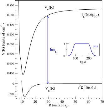
Figure 1: (Color online) $a^{3}\Sigma_{u}^{+}(6s,6s)$ and $1_{g}(6s,6p_{3/2})$ electronic potentials of Cs₂, coupled at a internuclear distance of about $R_{c}\approx 29\ a_{0}$ by a pulse with frequency $\omega_{L}/2\pi$ and envelope $e(t)$ shown in the inset. The energy origin is taken to be the dissociation limit $E_{6s+6s}=0$ of the $a^{3}\Sigma_{u}^{+}(6s,6s)$ potential.

This section will present results obtained from the simulation of the intramolecular dynamics for a diatomic molecule which is under the action of a laser pulse coupling two electronic states. Non-Markovian behavior of the electronic subsystem is characterized using the canonical measures of non-Markovianity $f(t)$ and $F(t_{1},t_{2})$$=\int_{t_{1}}^{t_{2}}f(t)dt$, calculated using the equations established in Sec. III.4. We will also examine the time behavior of the Bloch volume $\mathcal{V}(t)$ of the accessible states, obtained using Eqs. (68,69), as well as the dynamics of the electronic-vibrational entanglement and the electronic coherence in the molecule. Non-Markovian behavior during time evolution will be connected with the dynamics of quantum correlations.

As a model system, we consider the Cs₂ molecule in which the electronic states $g=a^{3}\Sigma_{u}^{+}(6s,6s)$ and $e=1_{g}(6s,6p_{3/2})$ are coupled by a laser pulse. In previous works Vatasescu et al. (2001); Vatasescu (2009, 2013) , we have analyzed the vibrational dynamics in these electronic potentials for various conditions of coupling, and we shall refer to these works for details of the molecular model, including definitions of the characteristic times of dynamics, such as vibrational and Rabi periods.

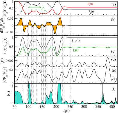
Figure 2: (Color online) Results characterizing the vibrational dynamics in the electronic potentials $g=a^{3}\Sigma_{u}^{+}$ and $e=1_{g}$ of Cs₂ coupled by a pulse with envelope $e(t)$ (Fig. 1), for a coupling strength $W_{L}=3.29$ cm^-1. Time evolutions during the pulse ($t<250$ ps) and after pulse ($t>250$ ps) are both shown. (a) Time evolution of the populations $P_{g}(t)$ and $P_{e}(t)$ (two specific Rabi periods $T^{R}_{v_{e},v_{g}}$, of $47.4$ ps and $16.5$ ps, are marked). (b) Time evolution of the ”non-Markovianity factor” $d(P_{g}P_{e})/dt$ (non-Markovianity is enhanced if $d(P_{g}P_{e})/dt>0$). (c) Time evolutions of the linear entropy $L(t)$ and von Neumann entropy $S_{vN}(t)$ of the electronic-vibrational entanglement. (d) Time evolution of the skew information $I_{S}(t)={\cal I_{S}}(R,t)/[\Delta V(R)]^{2}$. (e) Time evolution of the electronic coherence $C_{l_{1}}(t)/2=|<\psi_{g}(t)|\psi_{e}(t)>|$. (f) Non-Markovianity measure $f(t)$. The filled surface shows the integral $\int f(t)dt$.

Let us suppose the electronic states $g=a^{3}\Sigma_{u}^{+}(6s,6s)$ and $e=1_{g}(6s,6p_{3/2})$ coupled by an electric field with temporal amplitude ${\cal{E}}(t)={\cal{E}}_{0}e(t)\cos\omega_{L}t$. The field amplitude ${\cal{E}}_{0}=\sqrt{2I/c\epsilon_{0}}$ depends on the laser intensity $I$, $e(t)$ is the temporal envelope of the pulse, and $\omega_{L}/2\pi$ is the frequency of the field, such as the photon energy $\hbar\omega_{L}$ couples the electronic potentials $V_{g}(R)$ and $V_{e}(R)$ at a internuclear distance of about $R_{c}\approx 29\ a_{0}$, as it is shown in Fig. 1. Using the rotating wave approximation with the frequency $\omega_{L}/2\pi$, and a transformation of the radial wave functions with appropriate phase factors, one obtains the typical Eq. (30) for the vibrational wave packets $\psi_{g}(R,t)$ and $\psi_{e}(R,t)$ whose dynamics takes place in the diabatic electronic potentials crossing in $R_{c}$ Vatasescu et al. (2001). The coupling between the electronic channels is $W(t)=W_{L}e(t)$, with the strength $W_{L}=-\frac{1}{2}{\cal{E}}_{0}D_{ge}^{\vec{e_{L}}}$, where $D_{ge}^{\vec{e_{L}}}$ is the transition dipole moment between the ground $g$ and the excited $e$ electronic states, for a polarization ${\vec{e_{L}}}$ of the electric field Vatasescu et al. (2001). Here the $R$-dependence of the transition dipole moment is neglected, and several coupling strengths $W_{L}$ are considered, for the same pulse envelope $e(t)$ (represented in Fig. 1).

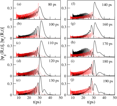
Figure 3: (Color online) Time evolution (80 - 190 ps) of the vibrational wave packets $|\Psi_{g}(R,t)|$ (full line) and $|\Psi_{e}(R,t)|$ (dotted line) in $g=a^{3}\Sigma_{u}^{+}(6s,6s)$ and $e=1_{g}(6s,6p_{3/2})$ electronic potentials coupled by a pulse with envelope $e(t)$ (Fig. 1), for a coupling strength $W_{L}=3.29$ cm^-1.

The intramolecular dynamics is obtained using Eq. (30), which is solved numerically by propagating in time an initial wave function (here the initial state is the vibrational eigenstate with $v_{e}=142$ of the $1_{g}(6s,6p_{3/2})$ potential) on a spatial grid with length $L_{R}$. The Mapped Sine Grid (MSG) method Luc-Koenig et al. (2004); Willner et al. (2004) is used to represent the radial dependence of the wave packets, and the time propagation uses the Chebychev expansion of the evolution operator Kosloff (1994, 1996). The electronic populations $P_{g}(t)$, $P_{e}(t)$ are calculated from the vibrational wave packets as $P_{g,e}(t)=\int^{L_{R}}|\Psi_{g,e}(R^{\prime},t)|^{2}dR^{\prime}$, and the electronic coherence (83) is obtained from the overlap of the vibrational wave packets calculated on the spatial grid: $<\psi_{g}(t)|\psi_{e}(t)>$$=\int^{L_{R}}\Psi^{*}_{g}(R^{\prime},t)\Psi_{e}(R^{\prime},t)dR^{\prime}$. These results are used to calculate the canonical decoherence rates and measures of non-Markovianity, as well as the entropies of the electronic-vibrational entanglement and the skew information.

We begin by analyzing dynamics for a coupling strength $W_{L}=3.29$ cm^-1 (corresponding to a pulse intensity $I\approx 2.7$ MW/cm² for a linear polarization vector ${\vec{e_{L}}}$ Vatasescu (1999)), for which the results are given in Figs. 2,3 and 4. Fig. 2 shows the time evolutions of several significant quantities: electronic populations $P_{g}(t)$, $P_{e}(t)$, ”non-Markovianity factor” $d(P_{g}P_{e})/dt$, entropies $L(t)$ and $S_{vN}(t)$ of the electronic-vibrational entanglement, electronic coherence $C_{l_{1}}(t)$ and skew information $I_{S}(t)$, as well as the non-Markovianity measure $f(t)$. The vertical dotted lines in the figure help us to observe the correlations between the temporal variations of all these properties. Figs. 3 and 4 show the time evolution of the vibrational wave packets $|\Psi_{g}(R,t)|$ and $|\Psi_{e}(R,t)|$, during the pulse and after pulse.

The pulse, which operates from 50 to 250 ps (see the envelope $e(t)$ in Fig. 1), couples the two electronic states activating a vibrational dynamics which involves several vibrational levels of each surface, with vibrational periods of about 11 ps in the $1_{g}$ electronic potential (the vibrational levels $v_{e}=140$ up to $143$ are implied), and between 33 and more than 100 ps in the $a^{3}\Sigma_{u}^{+}$ potential (corresponding mainly to the vibrational levels from $v_{g}=43$ up to $49$). The pulse produces a rich vibrational dynamics, implying transfer of population between the electronic states, inversion of population, and beats with various Rabi periods $T^{R}_{v_{e},v_{g}}$ Vatasescu (2009) between the populated vibrational levels of the excited and ground states. These phenomena are visible in Fig. 2(a), where typical Rabi periods can be identified, such as $T^{R}_{v_{e},v_{g}}=47.4$ ps (between $v_{e}=142$ of $1_{g}$ and $v_{g}=47$ of $a^{3}\Sigma_{u}^{+}$) and $T^{R}_{v_{e},v_{g}}=16.5$ ps (between $v_{e}=142$, $v_{g}=45$). The time evolution of the wave packets in Figs. 3 and 4 allows us to observe the relation between the population transfer between electronic channels and the vibrational motion in the potential wells. Let us briefly decipher the dynamics from these results. The pulse begins by transferring electronic population from $e=1_{g}$ state ($P_{e}(0)=1$) to $g=a^{3}\Sigma_{u}^{+}$ state, the populations becoming equals at about 80 ps. This process, taking place from 50 to 80 ps, increases entanglement (Fig. 2(c)), and is associated with a strong non-Markovian behavior (Fig. 2(f)). After 80 ps, $P_{g}(t)>P_{e}(t)$, and the population transfer from $e$ to $g$ continues with the diminution of the entanglement and the non-Markovianity measure $f(t)$. The inversion of population is almost completed at 100 ps, and the transfer is inverted, producing a non-Markovianity maximum between 100 and 110 ps (Fig. 2(f)), followed by stabilization of populations with small Rabi beatings between 110 and 130 ps. The vibrational motion inside the $a^{3}\Sigma_{u}^{+}$ potential empties the transfer zone located around the crossing point $R_{c}\approx 29\ a_{0}$ (see Fig. 3(f), t=140 ps), therefore between 130 and 140 ps the population is transferred from $1_{g}$ to $a^{3}\Sigma_{u}^{+}$, diminishing the entanglement and the function $f(t)$. Between 160 and 190 ps, the pulse again transfers again population from the $g=a^{3}\Sigma_{u}^{+}$ state to the $e=1_{g}$ state, increasing the entanglement and the non-Markovianity function $f(t)$ (this process is temporarily stopped around 170 ps by the vibration of the $g=a^{3}\Sigma_{u}^{+}$ packet, as shown in Fig. 3(h)). Finally, before the end of the pulse, the massive transfer of population from the $g=a^{3}\Sigma_{u}^{+}$ state to the $e=1_{g}$ state, between 200 and 220 ps, increases the entanglement and has a notable non-Markovian character (see Figs. 2(a,c,f) and 4(a-c)).

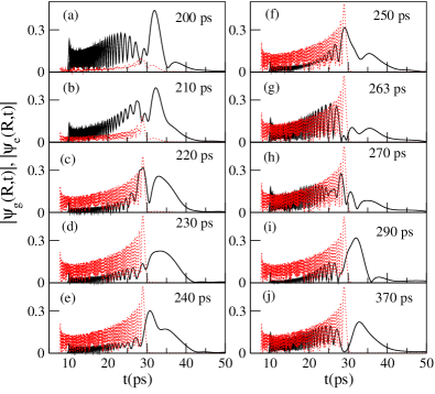
Figure 4: (Color online) Continuation of Fig. 3: time evolution (200 - 370 ps) of the vibrational wave packets $|\Psi_{g}(R,t)|$ (full line) and $|\Psi_{e}(R,t)|$ (dotted line) for a coupling $W_{L}=3.29$ cm^-1. (a-e) Time evolution during the pulse. (f-j) Time evolution after pulse.

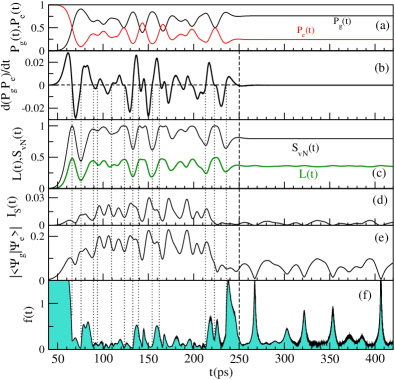
Figure 5: (Color online) Results for a coupling strength $4W_{L}=13.16$ cm^-1 between the electronic states $g=a^{3}\Sigma_{u}^{+}$ and $e=1_{g}$ of Cs₂ coupled by a pulse with the same envelope $e(t)$ shown in Fig. 1. Evolutions during the pulse and after pulse. (a) Time evolutions of the populations $P_{g}(t)$ and $P_{e}(t)$. (b) Time evolution of the ”non-Markovianity factor” $d(P_{g}P_{e})/dt$. (c) Time evolutions of the linear entropy $L(t)$ and von Neumann entropy $S_{vN}(t)$ of the electronic-vibrational entanglement. (d) Time evolution of the skew information $I_{S}(t)={\cal I_{S}}(R,t)/[\Delta V(R)]^{2}$. (e) Time evolution of the electronic coherence $C_{l_{1}}(t)/2=|<\psi_{g}(t)|\psi_{e}(t)>|$. (f) Non-Markovianity measure $f(t)$. The filled surface shows the integral $\int f(t)dt$.

Let us observe more closely the influence exerted by this dynamics of transfer and vibration on the non-Markovian character of the electronic evolution. Let us analyze the evolution during the pulse ($t<250$ ps). A first observation (see Figs. 2(b,c)) is that whenever the electronic-vibrational entanglement increases ($dL(t)/dt>0$, $dS_{vN}(t)/dt>0$), the ”non-Markovianity factor” is positive, $d(P_{g}P_{e})/dt>0$, and whenever entanglement decreases ($dL(t)/dt<0$, $dS_{vN}(t)/dt<0$), the ”non-Markovianity factor” is negative, $d(P_{g}P_{e})/dt<0$. There is no exception from this rule in this case, therefore we observe only the situations (2) and (4) from the Table  1. Secondly, Figs. 2(b,c,f) show clearly that, in the time intervals $[t_{1},t_{2}]$ when the condition of enhanced non-Markovian behavior $d(P_{g}P_{e})/dt>0$ is fulfilled (i.e. whenever there is entanglement growth), the total amount of non-Markovianity defined by the integral $F(t_{1},t_{2})$$=\int_{t_{1}}^{t_{2}}f(t)dt$ becomes significantly bigger (for example, the intervals 100-110 ps, 120-130 ps, 145-155 ps, 160-190 ps, or 203-220 ps). On the contrary, if the entanglement decreases during the time interval $[t_{1},t_{2}]$, $F(t_{1},t_{2})$ is drastically diminished, approaching 0 (between 130-145 ps, for example).

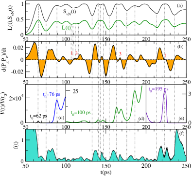
Figure 6: (Color online) Results during the pulse for a coupling $4W_{L}=13.16$ cm^-1.(a) Time evolutions of the linear entropy $L(t)$ and von Neumann entropy $S_{vN}(t)$ of the electronic-vibrational entanglement. (b) Time evolution of the ”non-Markovianity factor” $d(P_{g}P_{e})/dt$ (non-Markovianity is enhanced for $d(P_{g}P_{e})/dt>0$). (c-e) Time evolution of the Bloch volume of the accessible states relative to the volume at an initial time $t_{0}$, $\mathcal{V}(t)/\mathcal{V}(t_{0})$. Three time periods (with appropriated initial times $t_{0}$) are considered: (c) beginning of the pulse $[50-100]$ ps; (d) the period of constant strength $[100-195]$ ps; (e) end of the pulse, $[195-250]$ ps. (f) Non-Markovianity measure $f(t)$. The filled surface shows the integral $\int f(t)dt$.

After pulse ($t>250$ ps), the electronic populations become constant, and $d(P_{g}P_{e})/dt=0$. Vibrational motion in the electronic potentials leads to oscillations of the electronic coherence, and implicitly of the linear entropy $L(t)$. The non-Markovianity measure is deduced from Eq. (78) as $f(t)=$$\frac{1}{|<\psi_{g}|\psi_{e}>|}\left|\frac{d<\psi_{g}|\psi_{e}>}{dt}\right|$, taking the form (80) as function of the electronic coherence $|<\psi_{g}|\psi_{e}>|$. The results shown in Figs. 2(e,f) confirm the analysis made in Sec. III.4 for a molecule with constant electronic populations: indeed, the non-Markovianity measure $f(t)$ has minima when the electronic coherence $|<\psi_{g}|\psi_{e}>|$ has maxima (for example, at t=250 ps, 280 ps, 385 ps), and attains maximum values when $|<\psi_{g}|\psi_{e}>|\to 0$ (at t=263 ps or 370 ps, for example). Let us observe the wave packets evolution in Figs. 4(f-j): the minima of the electronic coherence are obtained when the overlap of the vibrational wave packets is minimum. As it can be seen for t=263 ps or 370 ps, the minimum overlap is a result of the $\psi_{g}(R,t)$ vibration inside the $a^{3}\Sigma_{u}^{+}$ potential. This vibrational motion (during which the vibrational wave packets explore the electronic potentials) diminishes coherence, increasing the electronic-vibrational entanglement and bringing a memory character to dynamics.

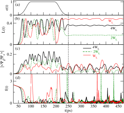
Figure 7: (Color online) Results for the coupling strengths $W_{L}=3.29$ cm^-1 (thin line), $2W_{L}$ (dashed line), and $4W_{L}$ (thick line) between the electronic states $g=a^{3}\Sigma_{u}^{+}$ and $e=1_{g}$ of Cs₂ (Fig. 1). The dashed vertical line at $t=250$ ps indicates the end of the pulse. (a) Pulse envelope $e(t)$. (b) Time evolution of the linear entropy $L(t)$ of the electronic-vibrational entanglement. (c) Time evolution of the electronic coherence $C_{l_{1}}(t)/2=|<\psi_{g}(t)|\psi_{e}(t)>|$. (d) Non-Markovianity measure $f(t)$.

Let us observe the evolution of the two ”electronic coherences”, $C_{l_{1}}(t)$ and the skew information $I_{S}(t)$, shown in Figs. 2(e,d), respectively. During the pulse, they manifest similar behaviors, so we do not observe the exceptions signaled in the Table  1 for the cases (2) and (4). After pulse, their temporal behaviors are also similar, but $I_{S}(t)\to 0$ in the time intervals for which $C_{l_{1}}(t)$ has small values (for example, 260-270 ps, or 360-370 ps). At the same time, these intervals are also the periods when the non-Markovianity measure $F(t_{1},t_{2})$$=\int_{t_{1}}^{t_{2}}f(t)dt$ attains the bigger values after pulse (see Figs. 2(d,e,f)).

We will now analyze the results obtained for a much bigger coupling strength, $4W_{L}=13.16$ cm^-1, which are shown in Figs. 5 (evolution during and after pulse) and 6 (detailed evolution during the pulse). The transfer of population between the electronic channels becomes more intense and fast, and then the ”non-Markovianity factor” $d(P_{g}P_{e})/dt$ varies more rapidly (Figs. 5(a,b)). As in the case discussed previously, the increase of the electronic-vibrational entanglement ($dL(t)/dt>0$, $dS_{vN}(t)/dt>0$) is completely correlated with the positivity of the ”non-Markovianity factor” ($d(P_{g}P_{e})/dt>0$) indicating enhanced non-Markovian behavior. Also, entanglement decrease corresponds to $d(P_{g}P_{e})/dt<0$. The dotted vertical lines in Figs. 5(b,c) and 6(a,b) clearly show these correlations. Nevertheless, in this case exceptions from this rule can be observed: indeed, as it is shown in Figs. 6(a,b), one can distinguish small periods of time corresponding to the cases (1) and (3) analyzed in the Table 1. Figs. 6(a,b,f) also show that, as previously, when entanglement increases and the condition $d(P_{g}P_{e})/dt>0$ is fulfilled, the integral $\int f(t)dt$ is significantly increased.

Table 2: The total amount of non-Markovianity over the time interval $[t_{i},t_{f}]$, $F(t_{i},t_{f})$$=\int_{t_{i}}^{t_{f}}f(t)dt$, calculated for various time intervals (during the pulse with the envelope $e(t)$ shown in Fig. 7(a), and after pulse), and for the strengths $W_{L}=3.29$ cm^-1, $2W_{L}$, and $4W_{L}$ of the coupling.

	$F$(50,100 ps)	$F$(100,195 ps)	$F$(195,250 ps)	$F$(50,250 ps)	$F$(250,495 ps)
$W_{L}$	57.6	74.6	98.3	187.3	53.2
$2W_{L}$	50.3	20.7	31.6	102.6	59.7
$4W_{L}$	36.8	16.1	22.3	75.2	58.9

Figs. 6(c-e) show time evolutions of the Bloch volume reported at an initial time $t_{0}$, $\mathcal{V}(t)/\mathcal{V}(t_{0})$, corresponding to three periods belonging to the time interval $[50,250]$ ps of the pulse action, and relative to different initial times $t_{0}$: (c) beginning of the pulse $[50-100]$ ps ($t_{0}=62$ ps, $t_{0}=76$ ps); (d) the period of constant strength $[100-195]$ ps ($t_{0}=100$ ps); (e) end of the pulse, $[195-250]$ ps ($t_{0}=195$ ps). From the theoretical analysis exposed in Sec. III.4, it is expected that the Bloch volume will increase, witnessing non-Markovianity, only if $d(P_{g}P_{e})/dt>0$. This is exactly what we observe in Figs. 6(a-f): increase of the Bloch volume is correlated to increase of entanglement, the condition of enhanced non-Markovian behavior $d(P_{g}P_{e})/dt>0$, and the increase of the integral $\int f(t)dt$.

Non-Markovianity evolution after pulse is shown in Fig. 5(f). The function $f(t)$ evolves in the manner previously analyzed, with pronounced maxima corresponding to the electronic coherence $|<\psi_{g}|\psi_{e}>|$ minima.

The results obtained for three strengths of the coupling ($W_{L}=3.29$ cm^-1, $2W_{L}$, and $4W_{L}$) and the same pulse envelope are compared in Fig. 7, which exposes the linear entropy $L(t)$ of the electronic-vibrational entanglement, the electronic coherence $|<\psi_{g}|\psi_{e}>|$, and the non-Markovianity measure $f(t)$. The total amount of non-Markovianity $F(t_{i},t_{f})$$=\int_{t_{i}}^{t_{f}}f(t)dt$ over the time interval $[t_{i},t_{f}]$ was calculated for several time intervals, corresponding to the beginning of the pulse ($[50,100]$ ps), the period of constant coupling ($[100,195]$ ps), the end of the pulse ($[195,250]$ ps), and after pulse ($[250,495]$ ps). The values given in the Table 2 show that the total amount of non-Markovianity corresponding to the pulse action, $F$(50,250 ps), decreases with the increase of the coupling $W_{L}$, but, after pulse, the values $F$(250,495 ps) calculated for the three strengths of the coupling attain similar values.

Therefore, we find that during the pulse action, it is the weaker pulse which stimulates the bigger amount of non-Markovianity. This behavior is related to the Rabi periods of the population exchange between electronic channels, with a weak coupling enabling a more powerful presence of the vibrational environment. Indeed, a strong coupling induces a stronger electronic coherence (see Fig. 7 (c)), favoring the transfer of population between channels (localized around the crossing point of the electronic potentials) over the vibrational motion in the molecular potentials. A fast transfer of population corresponding to a strong coupling (i.e. small Rabi period) has the effect of ”locking” the population in the transfer zone, inhibiting vibration. By contrast, a slower transfer of population, produced by a weak pulse, gives wave packets more time to explore the electronic potentials, increasing gradually the entanglement and enhancing non-Markovian behavior.

VII Conclusions

We have examined non-Markovian behavior in the reduced time evolution of the electronic subsystem of a laser-driven molecule, as an open quantum system entangled with the vibrational environment.

Non-Markovianity was characterized using the canonical measures defined in Ref. Hall et al. (2014) as functions of the negative decoherence rates appearing in the corresponding canonical master equation. The canonical measures provide a complete description of non-Markovian behavior, being sensitive to individual decoherence rates when several decoherence channels are present. The Bloch volume of accessible states was also considered as a non-Markovianity witness, even if it does not always detect non-Markovian behavior, being only sensitive to the sum of the decoherence rates Hall et al. (2014). The use of different non-Markovianity measures helped to highlight the enhanced non-Markovian behavior, detected by both measures and generally accompanied by the increase of the electronic-vibrational entanglement.

For a laser-driven molecule described in a bipartite Hilbert space $\cal{H}$$=$$\cal{H}$_el$\bigotimes$$\cal{H}$_vib with dimension $2\times N_{v}$, we have derived the canonical form of the electronic master equation, deducing the canonical decoherence rates as functions of the electronic populations $P_{g}(t),P_{e}(t)$ and of the electronic coherence (Eqs. (55), (56)). Subsequently, the canonical measures of non-Markovianity and the Bloch volume of dynamically accessible states were obtained. We found that one of the decoherence rates is always negative, accounting for the inherent non-Markovian character of the electronic evolution. Moreover, a second decoherence rate becomes negative if the condition $d(P_{g}P_{e})/dt>0$ is fulfilled, leading to enhanced non-Markovian behavior, characterized by two negative decoherence rates and a negative sum of the decoherence rates; consequently, the Bloch volume of accessible states increases, detecting enhanced non-Markovian behavior. Sec. III.4 contains a detailed examination of the canonical measures in relation to the time evolution of the electronic populations and electronic coherence.

We showed that in the case of a molecule with constant electronic populations, the non-Markovianity measure $f(t)$ can be seen as a measure of the temporal behavior of the electronic coherence (which determines the evolution of $L(t)$, the linear entropy of entanglement), having minima when the electronic coherence has maxima ($L(t)$ minima), and attaining maximum values whenever the overlap of the vibrational packets tends to zero ($L(t)$ maxima). This signifies that vibrational motion which explore the electronic potentials diminishing nuclear overlap (i.e. increasing the linear entropy of entanglement) brings a memory character to dynamics.

The condition $d(P_{g}P_{e})/dt>0$ was used as an instrument to explore the meaning of enhanced non-Markovian behavior in the evolution of the electronic subsystem, observing its connections to the dynamics of electronic-vibrational entanglement and electronic coherence in molecule. We have employed analytical formulas to analyze connections between $d(P_{g}P_{e})/dt$, the time behavior of linear entropy of entanglement ($dL/dt$), and behaviors of speakable and unspeakable Marvian and Spekkens (2016) electronic coherences, measured by $l_{1}$ norm $C_{l_{1}}(t)$ and skew information ${\cal I_{S}}(t)$, respectively. We have also discussed the possibility of relating the conditions $d(P_{g}P_{e})/dt>0$, $dL/dt>0$, or $dC_{l_{1}}/dt>0$ to a flow of information from the vibrational environment to the electronic open subsystem. In this respect, in the appendix we have examined the conditions determining the growth of distinguishability Breuer et al. (2009) between two electronic states. It appears that the condition $d(P_{g}P_{e})/dt>0$ of enhanced non-Markovian behavior participates in the increase of the trace distance $D(\hat{\rho}_{el}(t_{0}),\hat{\rho}_{el}(t))$, and is closely related to the condition of increase of entanglement, $dL(t)/dt>0$.

In the last part of the paper we have analyzed non-Markovian behavior in the reduced evolution of the electronic states $g=a^{3}\Sigma_{u}^{+}(6s,6s)$ and $e=1_{g}(6s,6p_{3/2})$ of the Cs₂ molecule, coupled by a laser pulse. The motion of the vibrational wave packets in the electronic molecular potentials coupled by the laser pulse was simulated numerically, for several strengths of the pulse. The non-Markovian behavior, characterized using the canonical measures and the Bloch volume, was analyzed in relation to dynamics of the electronic-vibrational entanglement and electronic coherence in the molecule. We found that increase of electronic-vibrational entanglement ($dL(t)/dt>0$, $dS_{vN}(t)/dt>0$) is correlated with the positivity of the non-Markovianity factor ($d(P_{g}P_{e})/dt>0$), indicating enhanced non-Markovian behavior, with the increase of the Bloch volume, and with the growth of the total amount of non-Markovianity over an interval $[t_{1},t_{2}]$, given by the integral $F(t_{1},t_{2})$$=\int_{t_{1}}^{t_{2}}f(t)dt$, where $f(t)$ is the canonical measure of non-Markovianity, defined from the appearance of negative decoherence rates in the canonical master equation.

We have shown that the total amount of non-Markovianity corresponding to the pulse action decreases with the increase of the coupling. Nevertheless, the values $F(t_{1},t_{2})$ corresponding to evolutions after pulses are similar, probably because analogous domains of vibrational levels are populated, and therefore a similar vibrational dynamics is activated. The fact that during the pulse action, it is the weaker pulse which stimulates the bigger amount of non-Markovianity, has to be related to the Rabi periods characterizing the exchange of population between electronic channels, and influencing vibration in the electronic potentials. A weak pulse gives more time to vibrational wave packets to explore the electronic potentials, leading to entanglement increase and enhancement of non-Markovianity.

In conclusion, in a molecule (here with two populated electronic states), the evolution of the electronic subsystem has an inherent non-Markovian character due to the dynamics of the vibrational environment, even if there is no exchange of population between electronic channels, but only vibrational motion in the electronic potentials. Enhanced non-Markovian behavior of the electronic dynamics arises if there is a coupling between electronic channels such that the evolution of electronic populations obeys $d(P_{g}P_{e})/dt>0$, and it appears as a dynamical property associated with the increase of the electronic-vibrational entanglement. Several non-Markovianity regimes, determined by the sign of the non-Markovianity factor $d(P_{g}P_{e})/dt$, were analyzed in Sec. III.4 and Sec. IV.

A key motivation shaping the present work was to examine non-Markovian behavior of the electronic evolution in relation to the dynamics of the quantum correlations in the molecular system. In this sense, observation of the correlation phenomena accompanying enhancement of non-Markovianity reveals appropriate ways to understand non-Markovian behavior. Therefore, if the non-Markovian character of the electronic dynamics cannot be separated from the presence of the electronic coherence, the most significant relation is between non-Markovianity and entanglement dynamics: We have shown that non-Markovianity of the electronic evolution is essentially a dynamical property generated during the increase of electronic-vibrational entanglement.

*

Appendix A Distinguishability between two electronic states, $\hat{\rho}_{el}(t_{0})$ and $\hat{\rho}_{el}(t)$

Distinguishability between two electronic states $\hat{\rho}_{el}(t_{0})$ and $\hat{\rho}_{el}(t)$ can be analyzed using as measure the trace distance $D(\hat{\rho}_{el}(t_{0}),\hat{\rho}_{el}(t))$ between the two states, defined as Breuer et al. (2009); Breuer (2012)

$$D(\hat{\rho}_{el}(t_{0}),\hat{\rho}_{el}(t))=\frac{1}{2}\text{Tr}_{el}|\hat{\rho}_{el}(t_{0})-\hat{\rho}_{el}(t))|.$$ (93)

Taking into account the matrix of the electronic density given by Eq. (34), one obtains Breuer (2012)

$$D(\hat{\rho}_{el}(t_{0}),\hat{\rho}_{el}(t))=\sqrt{[P_{g}(t_{0})-P_{g}(t)]^{2}+|C(t_{0})-C(t)|^{2}}.$$ (94)

In Eq. (94), $P_{g}(t_{0})-P_{g}(t)$ is the difference of the populations between $t_{0}$ and $t$, and $C(t_{0})-C(t)$ is the difference between the complex nondiagonal elements $C(t)$$=<\psi_{g}(t)|\psi_{e}(t)>=|C(t)|$exp$[i\alpha(t)]$ of the electronic density matrix (34) at $t_{0}$ and $t$. The $l_{1}$ norm measure of the electronic coherence is $C_{l_{1}}(\hat{\rho}_{el})$$=2|C(t)|$ .

We look for the conditions determining an increase of the trace distance, i.e. a positive rate of change $dD(\hat{\rho}_{el}(t_{0}),\hat{\rho}_{el}(t))/dt>0$. From Eq. (94) one obtains the following equation giving the rate of change of the trace distance, $dD(\hat{\rho}_{el}(t_{0}),\hat{\rho}_{el}(t))/dt$:

$$D(\hat{\rho}_{el}(t_{0}),\hat{\rho}_{el}(t))\frac{dD(\hat{\rho}_{el}(t_{0}),\hat{\rho}_{el}(t))}{dt}$$

$$=[P_{g}(t)-P_{g}(t_{0})]\frac{dP_{g}(t)}{dt}+|C(t)|\frac{d|C(t)|}{dt}$$

$$-|C(t_{0})|\frac{d|C(t)|}{dt}\text{cos}[\alpha(t_{0})-\alpha(t)]$$

$$-|C(t_{0})||C(t)|\text{sin}[\alpha(t_{0})-\alpha(t)]\frac{d\alpha(t)}{dt}.$$ (95)

As it could be expected, Eq. (95) shows that $dD(\hat{\rho}_{el}(t_{0}),\hat{\rho}_{el}(t))/dt$ is an oscillating function, which becomes positive or negative depending on the evolution at the instant $t$ and on the initial state at $t_{0}$. Nevertheless, some interesting observations can be made.

Let us consider the right hand side of Eq. (95). The first term becomes positive, $[P_{g}(t)-P_{g}(t_{0})]dP_{g}(t)/dt>0$, if $\text{sgn}(dP_{g}/dt)$$=\text{sgn}[P_{g}(t)-P_{g}(t_{0})]$, i.e. on those intervals $[t_{0},t]$ of the time evolution on which a smaller population at $t_{0}$ is increased at $t$ ($P_{g}(t_{0})<P_{g}(t)$, $dP_{g}(t)/dt>0$) or a larger population at $t_{0}$ is diminished at $t$ ($P_{g}(t_{0})>P_{g}(t)$, $dP_{g}(t)/dt<0$). In Sec. III.4 we have shown that the condition $(P_{g}-P_{e})$$dP_{g}/dt$ $<0$ of enhanced non-Markovian behavior is fulfilled when the transfer of population between the two electronic channels is such as the larger population decreases (i.e. the smaller electronic population increases). Moreover, this is also the condition leading to the increase of the electronic-vibrational entanglement. Therefore, our observation is that on time intervals $[t_{0},t]$ when the condition $(P_{g}-P_{e})$$dP_{g}/dt$ $<0$ ($d(P_{g}P_{e})/dt>0$) is fulfilled, also $[P_{g}(t)-P_{g}(t_{0})]dP_{g}(t)/dt>0$.

The second term on the right hand side of Eq. (95) is equal to $(C_{l_{1}}dC_{l_{1}}/dt)/4$, and it becomes positive if the electronic coherence increases, $dC_{l_{1}}/dt>0$.

The last two terms on the right hand side of Eq. (95) depend on the ”complex coherences” $C(t_{0})$ and $C(t)$, and can be characterized as ”easily oscillating” terms, whose signs are rapidly changing.

Let us suppose that the electronic state $\hat{\rho}_{el}(t_{0})$ is a state with electronic coherence $|C(t_{0})|=0$. Therefore, the last two terms become 0, and Eq. (95) shows that the trace distance between $\hat{\rho}_{el}(t_{0})$ and another state $\hat{\rho}_{el}(t)$ will increase ($dD(\hat{\rho}_{el}(t_{0}),\hat{\rho}_{el}(t))/dt>0$) in a interval $[t_{0},t]$ in which the conditions $d(P_{g}P_{e})/dt>0$ and $dC_{l_{1}}/dt>0$ are fulfilled. In other words, distinguishability between $\hat{\rho}_{el}(t)$ and a state $\hat{\rho}_{el}(t_{0})$ with coherence $C_{l_{1}}(t_{0})=0$ is increased when $d(P_{g}P_{e})/dt>0$ and $dC_{l_{1}}/dt>0$. Breuer, Laine and Piilo Breuer et al. (2009) interpret the growth of distinguishability between two states of the open system as the signature of a reversed flow of information from the environment back to the open system, an essential trait of non-Markovian behavior.

References

- Breuer and Petruccione (2002) H. P. Breuer and F. Petruccione, The Theory of Open Quantum Systems (Oxford University Press, Oxford, 2002).
- Breuer (2012) H. P. Breuer, J. Phys. B.: At. Mol. Opt. Phys. 45, 154001 (2012).
- Rivas et al. (2014) A. Rivas, A. F. Huelga, and M. B. Plenio, Rep. Prog. Phys. 77, 094001 (2014).
- Breuer et al. (2016) H. P. Breuer, E. M. Laine, and J. Piilo, Rev. Mod. Phys. 88, 021002 (2016).
- de Vega and Alonso (2017) I. de Vega and D. Alonso, Rev. Mod. Phys. 89, 015001 (2017).
- Pollock et al. (2018a) F. A. Pollock, C. Rodríguez-Rosario, T. Frauenheim, M. Paternostro, and K. Modi, Phys. Rev. Lett. 120, 040405 (2018a).
- Chakraborty (2018) S. Chakraborty, Phys. Rev. A 97, 032130 (2018).
- Li et al. (2018) L. Li, M. J. W. Hall, and H. M. Wiseman, Phys. Rep. 759, 1 (2018).
- Wolf et al. (2008) M. M. Wolf, J. Eisert, T. S. Cubitt, and J. I. Cirac, Phys. Rev. Lett. 101, 150402 (2008).
- Breuer et al. (2009) H. P. Breuer, E. M. Laine, and J. Piilo, Phys. Rev. Lett. 103, 210401 (2009).
- Rivas et al. (2010) A. Rivas, S. F. Huelga, and M. B. Plenio, Phys. Rev. Lett. 105, 050403 (2010).
- Lu et al. (2010) X. M. Lu, X. Wang, and C. P. Sun, Phys. Rev. A 82, 042103 (2010).
- Fanchini et al. (2014) F. F. Fanchini, G. Karpat, B. Çakmak, L. K. Castelano, G. H. Aguilar, O. J. Farías, S. P. Walborn, P. H. S. Ribeiro, and M. C. de Oliveira, Phys. Rev. Lett. 112, 210402 (2014).
- Debarba and Fanchini (2017) T. Debarba and F. F. Fanchini, Phys. Rev. A 96, 062118 (2017).
- Luo et al. (2012) S. Luo, S. Fu, and H. Song, Phys. Rev. A 86, 044101 (2012).
- Lorenzo et al. (2013) S. Lorenzo, F. Plastina, and M. Paternostro, Phys. Rev. A 88, 88, 020102(R) (2013).
- Hall et al. (2014) M. J. W. Hall, J. D. Cresser, L. Li, and E. Andersson, Phys. Rev. A 89, 042120 (2014).
- Chruściński et al. (2017) D. Chruściński, C. Macchiavello, and S. Maniscalco, Phys. Rev. Lett. 118, 080404 (2017).
- Pollock et al. (2018b) F. A. Pollock, C. Rodríguez-Rosario, T. Frauenheim, M. Paternostro, and K. Modi, Phys. Rev. A 97, 012127 (2018b).
- Addis et al. (2014) C. Addis, B. Bylicka, D. Chruściński, and S. Maniscalco, Phys. Rev. A 90, 052103 (2014).
- Chruściński and Maniscalco (2014) D. Chruściński and S. Maniscalco, Phys. Rev. Lett. 112, 120404 (2014).
- Neto et al. (2016) A. C. Neto, G. Karpat, and F. F. Fanchini, Phys. Rev. A 94, 032105 (2016).
- Huelga et al. (2012) S. F. Huelga, A. Rivas, and M. B. Plenio, Phys. Rev. Lett. 108, 160402 (2012).
- Orieux et al. (2015) A. Orieux, A. D’Arrigo, G. Ferranti, R. L. Franco, G. Benenti, E. Paladino, G. Falci, F. Sciarrino, and P. Mataloni, Sci. Rep. 5, 8575 (2015).
- Poyatos et al. (1996) J. F. Poyatos, J. I. Cirac, and P. Zoller, Phys. Rev. Lett. 77, 4728 (1996).
- Myatt et al. (2000) C. J. Myatt, B. E. King, Q. A. Turchette, C. A. Sackett, D. Kielpinski, W. M. Itano, C. Monroe, and D. J. Wineland, Nature 403, 269 (2000).
- Liu et al. (2011) B.-H. Liu, L. Li, Y.-F. Huang, C.-F. Li, G.-C. Guo, E.-M. Laine, H.-P. Breuer, and J. Piilo, Nat. Phys. 7, 931 (2011).
- Tang et al. (2012) J.-S. Tang, C.-F. Li, Y.-L. Li, X.-B. Zou, G.-C. Guo, H.-P. Breuer, E.-M. Laine, and J. Piilo, Europhys. Lett. 97, 10002 (2012).
- Cosco et al. (2018) F. Cosco, M. Borrelli, J. J. Mendoza-Arenas, F. Plastina, D. Jaksch, and S. Maniscalco, Phys. Rev. A 97, 040101(R) (2018).
- Bylicka et al. (2014) B. Bylicka, D. Chruściński, and S. Maniscalco, Sci. Rep. 4, 5720 (2014).
- Dong et al. (2018) Y. Dong, Y. Zheng, S. Li, C.-C. Li, X.-D. Chen, G.-C. Guo, and F.-W. Sun, npj Quantum Inf. 4, 3 (2018).
- Escher et al. (2011) B. M. Escher, R. L. de Matos Filho, and L. Davidovich, Nat. Phys 7, 406 (2011).
- Chin et al. (2012) A. W. Chin, S. F. Huelga, and M. B. Plenio, Phys. Rev. Lett. 109, 233601 (2012).
- Schmidt et al. (2015) R. Schmidt, M. F. Carusela, J. P. Pekola, S. Suomela, and J. Ankerhold, Phys. Rev. B 91, 224303 (2015).
- Chen and Goan (2016) C.-C. Chen and H.-S. Goan, Phys. Rev. A 93, 032113 (2016).
- Poggi et al. (2017) P. M. Poggi, F. C. Lombardo, and D. A. Wisniacki, EPL 118, 20005 (2017).
- Sampaio et al. (2017) R. Sampaio, S. Suomela, R. Schmidt, and T. Ala-Nissila, Phys. Rev. A 95, 022120 (2017).
- Meier and Tannor (1999) C. Meier and D. J. Tannor, J. Chem. Phys. 111, 3365 (1999).
- Gaspard and Nagaoka (1999) P. Gaspard and M. Nagaoka, J. Chem. Phys. 111, 5676 (1999).
- Kleinekathöfer (2004) U. Kleinekathöfer, J. Chem. Phys. 121, 2505 (2004).
- Welack et al. (2006) S. Welack, M. Schreiber, and U. Kleinekathöfer, J. Chem. Phys. 124, 044712 (2006).
- Roden et al. (2009) J. Roden, A. Eisfeld, W. Wolff, and W. T. Strunz, Phys. Rev. Lett. 103, 058301 (2009).
- Pomyalov et al. (2010) A. Pomyalov, C. Meier, and D. J. Tannor, Chem. Phys. 370, 98 (2010).
- Mangaud et al. (2017) E. Mangaud, C. Meier, and M. Desouter-Lecomte, Chem. Phys. 494, 90 (2017).
- Rebentrost et al. (2009a) P. Rebentrost, M. Mohseni, I. Kassal, S. Lloyd, and A. Aspuru-Guzik, New J. Phys. 11, 033003 (2009a).
- Kilgour and Segal (2015) M. Kilgour and D. Segal, J. Chem. Phys. 143, 024111 (2015).
- Sowa et al. (2017) J. K. Sowa, J. A. Mol, G. A. D. Briggs, and E. M. Gauger, Phys. Chem. Chem. Phys. 19(43), 29534 (2017).
- Rebentrost et al. (2009b) P. Rebentrost, R. Chakraborty, and A. Aspuru-Guzik, J. Chem. Phys. 131, 184102 (2009b).
- Burghardt et al. (2009) I. Burghardt, V. May, D. A. Micha, and E. R. Bittner, eds., Energy Transfer Dynamics in Biomaterial Systems (Springer, 2009).
- Reich et al. (2015) D. M. Reich, N. Katz, and C. P. Koch, Sci. Rep. 5, 12430 (2015).
- Puthumpally-Joseph et al. (2017) R. Puthumpally-Joseph, O. Atabek, E. Mangaud, M. Desouter-Lecomte, and D. Sugny, Mol. Phys. 115, 1944 (2017).
- Puthumpally-Joseph et al. (2018) R. Puthumpally-Joseph, E. Mangaud, V. Chevet, M. Desouter-Lecomte, D. Sugny, and O. Atabek, Phys. Rev. A 97, 033411 (2018).
- Mangaud et al. (2018) E. Mangaud, R. Puthumpally-Joseph, D. Sugny, C. Meier, O. Atabek, and M. Desouter-Lecomte, New J. Phys. 20, 043050 (2018).
- Vacher et al. (2017) M. Vacher, M. J. Bearpark, M. A. Robb, and J. P. Malhado, Phys. Rev. Lett. 118, 083001 (2017).
- Arnold et al. (2018) C. Arnold, O. Vendrell, R. Welsch, and R. Santra, Phys. Rev. Lett. 120, 123001 (2018).
- Mohseni et al. (2014) M. Mohseni, Y. Omar, G. S. Engel, and M. B. Plenio, eds., Quantum Effects in Biology (Cambridge University Press, 2014).
- Roden et al. (2012) J. Roden, W. T. Strunz, K. B. Whaley, and A. Eisfeld, J. Chem. Phys. 137, 204110 (2012).
- Roden and Whaley (2016) J. J. J. Roden and K. B. Whaley, Phys. Rev. E 93, 012128 (2016).
- Roden et al. (2016) J. J. J. Roden, D. I. G. Bennett, and K. B. Whaley, J. Chem. Phys. 144, 245101 (2016).
- Ishizaki et al. (2010) A. Ishizaki, T. R. Calhoun, G. S. Schlau-Cohen, and G. R. Fleming, Phys. Chem. Chem. Phys. 12, 7319 (2010).
- Rebentrost and Aspuru-Guzik (2011) P. Rebentrost and A. Aspuru-Guzik, J. Chem. Phys. 134, 101103 (2011).
- Chen et al. (2014) H.-B. Chen, J.-Y. Lien, C.-C. Hwang, and Y.-N. Chen, Phys. Rev. E 89, 042147 (2014).
- Chen et al. (2015) H.-B. Chen, N. Lambert, Y.-C. Cheng, Y.-N. Chen, and F. Nori, Sci. Rep. 5, 12753 (2015).
- Note (1) We emphasize that here we are referring to entanglement between the electronic system and its vibrational environment, and not to entanglement with an ancilla, proposed in Ref. Rivas et al. (2010) as a non-Markovianity measure.
- Wolf and Cirac (2008) M. M. Wolf and J. I. Cirac, Commun. Math. Phys. 279, 147 (2008).
- Wißmann et al. (2015) S. Wißmann, H. P. Breuer, and B. Vacchini, Phys. Rev. A 92, 042108 (2015).
- Nakajima (1958) S. Nakajima, Prog. Theor. Phys. 20, 948 (1958).
- Zwanzig (1960) R. Zwanzig, J. Chem. Phys. 33, 1338 (1960).
- Shibata et al. (1977) F. Shibata, Y. Takahashi, and N. Hashitsume, J. Stat. Phys. 17, 171 (1977).
- Chaturvedi and Shibata (1979) S. Chaturvedi and F. Shibata, Z. Phys. B 35, 297 (1979).
- Breuer et al. (1999) H. P. Breuer, B. Kappler, and F. Petruccione, Phys. Rev. A 59, 1633 (1999).
- Strunz et al. (1999) W. T. Strunz, L. Diósi, and N. Gisin, Phys. Rev. Lett. 82, 1801 (1999).
- Breuer (2004) H. P. Breuer, Phys. Rev. A 70, 012106 (2004).
- Chruściński and Kossakowski (2010) D. Chruściński and A. Kossakowski, Phys. Rev. Lett. 104, 070406 (2010).
- Gorini et al. (1976) V. Gorini, A. Kossakowski, and E. C. G. Sudarshan, J. Math. Phys. 17, 821 (1976).
- Lindblad (1976) G. Lindblad, Commun. Math. Phys. 48, 119 (1976).
- Megier et al. (2017) N. Megier, D. Chruściński, J. Piilo, and W. T. Strunz, Sci. Rep. 7, 6379 (2017).
- Wiseman and Milburn (1993) H. M. Wiseman and G. J. Milburn, Phys. Rev. A 47, 1652 (1993).
- Piilo et al. (2008) J. Piilo, S. Maniscalco, K. Härkönen, and K.-A. Suominen, Phys. Rev. Lett. 100, 180402 (2008).
- Vatasescu (2013) M. Vatasescu, Phys. Rev. A 88, 063415 (2013).
- Vatasescu (2015) M. Vatasescu, Phys. Rev. A 92, 042323 (2015).
- Vatasescu (2016) M. Vatasescu, Phys. Rev. A 93, 069906(E) (2016).
- Lefebvre-Brion and Field (2004) H. Lefebvre-Brion and R. Field, The Spectra and Dynamics of Diatomic Molecules (Elsevier Academic Press, 2004).
- Note (2) In a general manner, can be an external coupling (the case of a laser pulse), or an internal coupling (such as a radial nonadiabatic coupling between electronic states), or a combination of both.
- Baumgratz et al. (2014) T. Baumgratz, M. Cramer, and M. B. Plenio, Phys. Rev. Lett. 113, 140401 (2014).
- Note (3) The theoretical model treating the relative motion of the nuclei in the ground and excited electronic channels coupled by a laser pulse usually contains supplementary assumptions, involving the rotating wave approximation and dressed electronic potentials Vatasescu et al. (2001); Vatasescu (2009, 2012).
- Marvian and Spekkens (2016) I. Marvian and R. W. Spekkens, Phys. Rev. A 94, 052324 (2016).
- Marvian et al. (2016) I. Marvian, R. W. Spekkens, and P. Zanardi, Phys. Rev. A 93, 052331 (2016).
- Streltsov et al. (2017) A. Streltsov, G. Adesso, and M. B. Plenio, Rev. Mod. Phys. 89, 041003 (2017).
- Note (4) The term “unspeakable coherence“ derives from the syntagm “unspeakable information“, which designates an information which can only be encoded in certain degrees of freedom Marvian and Spekkens (2016). Also following Ref. Marvian and Spekkens (2016), “speakable information is information for which the means of encoding is irrelevant“ (p. 2). The term “unspeakable coherence“ refers to the notion of “coherence as asymmetry“, and the term “speakable coherence“ is applied to the concept of coherence defined in the recently developed framework of resource theories of quantum coherence Marvian and Spekkens (2016); Marvian et al. (2016); Streltsov et al. (2017). It was shown that measures of coherence are a subset of measures of asymmetry Marvian et al. (2016).
- Luo (2005a) S. L. Luo, Theor. Math. Phys. 143, 681 (2005a).
- Luo (2005b) S. Luo, Phys. Rev. A 72, 042110 (2005b).
- Luo (2006) S. Luo, Phys. Rev. A 73, 022324 (2006).
- Vatasescu et al. (2001) M. Vatasescu, O. Dulieu, R. Kosloff, and F. Masnou-Seeuws, Phys. Rev. A 63, 033407 (2001).
- Vatasescu (2009) M. Vatasescu, J. Phys. B: At. Mol. Opt. Phys. 42, 165303 (2009).
- Luc-Koenig et al. (2004) E. Luc-Koenig, M. Vatasescu, and F. Masnou-Seeuws, Eur. Phys. J. D. 31, 239 (2004).
- Willner et al. (2004) K. Willner, O. Dulieu, and F. Masnou-Seeuws, J. Chem. Phys. 120, 548 (2004).
- Kosloff (1994) R. Kosloff, Annu. Rev. Phys. Chem. 45, 145 (1994).
- Kosloff (1996) R. Kosloff, “Quantum molecular dynamics on grids,” in Dynamics of Molecules and Chemical Reactions, edited by R. E. Wyatt and J. Z. Zhang (Marcel Dekker, New York, 1996) pp. 185–230.
- Vatasescu (1999) M. Vatasescu, Ph.D. thesis, Université Paris XI (1999).
- Vatasescu (2012) M. Vatasescu, Nucl. Instrum. Methods Phys. Res. B 279, 8 (2012).