2HDME: Two-Higgs-Doublet Model Evolver

Abstract

Two-Higgs-Doublet Model Evolver (2HDME) is a C++ program that provides the functionality to perform fast renormalization group equation running of the general, potentially $\mathcal{CP}$-violating, 2 Higgs Doublet Model at 2-loop order. Simple tree-level calculations of masses; calculations of the oblique parameters $S$, $T$ and $U$; different parameterizations of the scalar potential; tests of perturbativity, unitarity and tree-level stability of the scalar potential are also implemented. We briefly describe the 2HDME’s structure, provide a demonstration of how to use it and list some of the most useful functions.

PROGRAM SUMMARY

Program Title: 2HDME
Licensing provisions: GNU GPLv3
Programming language: C++
Nature of problem: Renormalization group evolution of the general, potentially complex, 2 Higgs doublet model at 2-loop order. Also tests of perturbativity, unitarity and tree-level stability of the model.
Solution method: Numerical solutions of systems of ordinary differential equations.

1 Introduction

The discovery of a 125 GeV scalar particle at the LHC [1, 2] marks the beginning of an era of precision Higgs physics. So far, it resembles the Higgs boson of the Standard Model (SM) [3]; however, further experimental investigation is required to decipher its true nature.

The Two-Higgs-Doublet Model (2HDM) is a very popular extension of the standard model. By adding a second Higgs doublet, it offers a rich phenomenology with three neutral and one charged pair of Higgs bosons. Some of its features are the possibility of explicit and spontaneous $\mathcal{CP}$-violation in the scalar sector; a dark matter candidate and lepton number violation. For a review of the 2HDM, we refer to ref. [4].

A useful tool when investigating the 2HDM is to employ a renormalization group (RG) analysis. One can with such a method look for instabilities, fine-tuning and valid energy ranges in the 2HDM’s parameter space. The RG equations (RGEs) for any renormalizable quantum field theory at 2-loop order are well known [5, 6, 7, 8]. However, implementing them for a specific model to perform numerical calculations is a tedious and error-prone task.

The purpose of 2 Higgs Doublet Model Evolver (2HDME) is to provide a fast C++ application programming interface (API) that can be used to evolve the 2HDM in renormalization scale by numerically solving its RGEs. 2HDME works with the general, potentially complex and $\mathcal{CP}$-violating, 2HDM and both 1- and 2-loop RGEs are implemented. Furthermore, calculations of oblique parameters, tests of perturbativity, unitarity and tree-level stability of the scalar potential are available.

In this manual, we give instructions and showcase some of 2HDME’s functionalities. The source code can be found at ref. [9] and we give some installation instructions in A. For a physics discussion, we refer to ref. [10]; which employs 2HDME to analyze $\mathbb{Z}_{2}$ breaking effects in the evolution of the 2HDM.

We begin by briefly describing the structure of 2HDME in section 2 and a demonstration of how to use the API is given in section 3; installation instructions are given in A. Further details on the base classes and the functionality they provide are then given in section 4. The main class of 2HDME is THDM which is described in section 5, where we also give a short review of the physics of the 2HDM. We give a short description of the algorithm used when performing RG evolution in section 6. Instructions of how to implement one’s own model or extend the THDM class are given in section 7. Finally, we discuss other software that are capable of performing RG evolution in section 8 and conclude in section 9.

2 Structure of 2HDME

2HDME is written in C++11 and depends on GSL [11] for numerically solving the RGEs as well as on Eigen [12] for linear algebra operations, see A for installation instructions. All source code is fairly well documented with comments in the header files, which show the functionality of all the classes. 2HDME originated from an extension of 2HDMC [13] and hence share a similar structure.

The purpose of 2HDME is to provide an API that consists of methods to manipulate a 2HDM model; thus the idea is that the user should write their own executable code that uses the THDM class of 2HDME. A simple example that demonstrates how to use 2HDME is provided in src/demos/DemoRGE.cpp; which is explained in more detail in section 3.

The main class of the 2HDME is the THDM object that describes a general, potentially complex, 2HDM; see section 5 for a more detailed description of its functionality. For basic usage, one only needs to interact with the public methods of THDM (and the SM class to set boundary conditions). The framework to solve RGEs is contained in the RgeModel class, which THDM inherits from. The RgeModel, furthermore, inherits some basic functionality related to data and console output from the abstract class BaseModel. To initialize a THDM object, one needs to specify three sectors: the Standard Model (SM) parameters, the scalar potential and the Yukawa sector.

The SM parameters that need to be set are the Higgs vacuum expectation value, fermion masses, CKM matrix, gauge couplings and renormalization scale at which they are defined. This can be done manually with a member function, where the user specifies all the input. Another method is to initialize the THDM class using the SM class that represents the SM. The SM is by default initialized at the top mass scale, $\approx$173 GeV, see C for a detailed list of all the values; however, these can all be easily changed using its member functions. Similar to the THDM, the SM also inherits RGE functionality from the RgeModel class, with its own set of RGEs. Thus, if one wants the SM parameters at another renormalization scale, the SM can be evolved to an arbitrary energy scale. However, one should only run models above the top mass scale, since the RGEs specified for the SM include all particles.

After setting up all the SM parameters, the THDM needs a scalar potential and a Yukawa sector. The scalar sector can be specified with any of the 2HDM bases in section B; these bases are separate structs that are defined in THDM_bases.cpp. Note though that THDM internally works in the generic basis.

The Yukawa sector can be specified in three ways. One option is to impose a $\mathbb{Z}_{2}$ symmetry; type-I,-II,-III(Y) or -IV(X); these are defined in table 1. Another is to use a flavor alignment ansatz, where the Yukawa matrices for the different Higgs fields are proportional to each other. Of course one can also set the Yukawa matrices manually as a third option.

To evolve the THDM or SM, one simply uses their member function evolve(). The options for the RG evolution can be set with the RgeConfig struct.

2.1 2-loop RGEs

The 2-loop RG equations (RGEs) for massless parameters of any renormalizable quantum field theory in 4 dimensions were derived in the seminal papers by Machacek and Vaughn [5, 6, 7]. That work has been supplemented with the 2-loop RGEs of massive parameters in ref. [8], which is the source that we have used to derive the 1- and 2-loop RGEs for a general 2HDM. Note though, that when working with quantum field theories with multiple indistinguishable scalar fields one must be careful when interpreting their formulas, since the formulas in ref. [5, 6, 7, 8] are written for the case of an irreducible representation of the scalar fields . In the case of a general 2HDM, one gets non-diagonal anomalous dimensions that mixes the scalar fields during RG evolution.

The general 2-loop RGEs are very long and we will thus not write them down here, but are instead provided as supplementary material and are of course also available in C++ format in the source code of 2HDME.

3 Demonstration of usage

As an example of how to use the 2HDME API, we here go through the DemoRGE in src/demos, where a 2HDM is initialized at the top mass scale and then evolved up to the Planck scale. For instructions of how to install and run the demo, see A.

The first thing to note is that the 2HDME is wrapped in a namespace, thus including using namespace THDME is convenient.

To initialize the THDM, we first need to specify the SM parameters. Rather then specifying them manually, we can use the SM class to provide all the necessary inputs. It is constructed at the top mass scale and we print its parameters to the console with SM sm;
sm.print_all(); This SM is used to initialize the CKM matrix, fermion mass $\kappa^{F}$ matrices, gauge couplings, vacuum expectation value (VEV) $v$ and the renormalization scale of the THDM. For instructions of how to obtain a SM at another renormalization scale, see section 4.3. Note, that the SM parameters can also be set manually with member functions that are described in section 4.3.3.

To create a THDM and feed it a SM, use THDM thdm(sm); Next up, we need to set the scalar potential. This can be done with any of the bases in section B. The bases are defined as struct objects which have member functions that can be used to convert one base to another. Here, we use the generic basis which we specify by Base_generic gen;
gen.beta = 1.46713;
gen.M12 = std::complex<double>(3132.85, 0.);
gen.Lambda1 = 0.413702;
gen.Lambda2 = 0.263926;
gen.Lambda3 = 0.13313;
gen.Lambda4 = -0.0444794;
gen.Lambda5 = std::complex<double>(0.29586, 0.);
gen.Lambda6 = std::complex<double>(0., 0.);
gen.Lambda7 = std::complex<double>(0., 0.); We set the potential with thdm.set_param_gen(gen); Finally we set the Yukawa sector to be type I $\mathbb{Z}_{2}$ symmetric with thdm.set_yukawa_type(TYPE_I);

Now that we have fully initialized the THDM and the SM, we can save them in SLHA-like text files with sm.write_slha_file();
thdm.write_slha_file();

To evolve the THDM, we need to configure the settings of the RG evolution. This is done by creating a RgeConfig struct and feeding it to the THDM like RgeConfig options;
options.dataOutput = true;
options.consoleOutput = true;
options.evolutionName = "DemoRGE";
options.twoloop = true;
options.perturbativity = true;
options.stability = false;
options.unitarity = false;
options.finalEnergyScale = 1e18;
options.steps = 100;
thdm.set_rgeConfig(options); The different options are explained in section 4.2. One can print the options to the console with options.print(). Now, we are ready to evolve the THDM with thdm.evolve(); which should only take a couple of seconds at 2-loop order. The parameters as functions of the renormalization scale are listed in output/DemoRGE/data and basic plots are created in output/DemoRGE/plots, see figure 1 for an example.

Afterwards we can print the parameters at the energy scale where the RG running stopped with thdm.print_all();. To retrieve the scalar potential, one can for example use thdm.get_param_gen();

Next up, we can evolve the THDM to another energy. First we save the THDM at the high scale with thdm.write_slha_file(sphenoLoopOrder, "DemoRGE_evolvedThdm");. It is always possible to evolve the thdm further. After the fist evolution, the THDM is specified at the high scale and to evolve the it downwards to $\mu=1$ TeV, all one has to do is to change the finalEnergyScale of its RgeConfig before evolving, which is achieved with options.finalEnergyScale = 1e3;
options.dataOutput = false;
thdm.set_rgeConfig( options);
thdm.evolve(); where we also changed dataOutput to false; thus preventing that the first plots are overwritten. A more compact method would be to use thdm.evolve_to(1e3), which sets the final scale to the given argument.

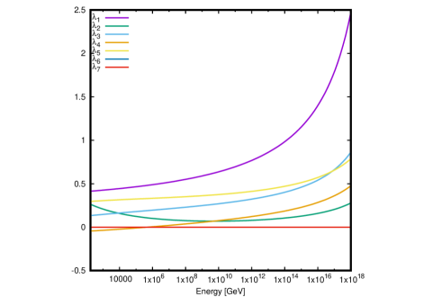
Figure 1: The evolution of quartic couplings in the generic basis produced by DemoRGE.cpp.

4 Classes

There are two main classes of 2HDME: THDM and SM. These inherit the features from the base classes BaseModel and RgeModel like

$$\text{{BaseModel}}\leftarrow~{} \text{{RgeModel}}\leftarrow\text{{THDM}},$$

$$\text{{BaseModel}}\leftarrow~{} \text{{RgeModel}}\leftarrow\text{{SM}}.$$

We briefly describe the features of the BaseModel, RgeModel and SM in the following subsections, while the THDM is described in more detail in section 5.

4.1 BaseModel class

The BaseModel is an abstract class that offers some basic functionality such as input and output to data files as well as to the console.

The level of information printed to the console of the THDM  and SM during computations can be set by

Function	Description	Returns
set_logLevel(LogLevel)	Sets level of console output information	void

where LogLevel can be either one of the following:

• LOG_INFO: Prints information of calculations performed and status updates.

• LOG_ERRORS: Only prints error messages.

• LOG_WARNINGS: Prints error messages and warning messages.

• LOG_DEBUG: Prints all the information as well as additional debugging information.

4.2 RgeModel class

The RgeModel inherits the input/output functionality of the BaseModel and acts as a base class which offers a framework to incorporate RG evolution in derived classes; both THDM and SM are derived classes of RgeModel.

If one wants to create a new type of class that implements RGE functionality similar to THDM and SM, it is easy to use RgeModel. For example one might want to extend the 2HDM with additional operators and consequently new parameters and RGEs. Instructions of how to do this is given in section 7. There is also the class NewModel, that serves as a minimalistic example of a new class that inherits from RgeModel.

See the header file RgeModel.h for a list of all member functions. Some of the most important ones are:

Function	Description	Returns
set_rgeConfig(RgeConfig)	Sets up the options for the RG evolution.	void
get_rgeConfig()	Retrieves the RG evolution options.	RgeConfig

The options for performing RG evolution are saved in the RgeConfig member variable _rgeConfig. This RgeConfig has the following member variables:

• bool twoloop: If true, uses 2-loop RGEs; otherwise uses 1-loop.

• bool perturbativity: If true, the RG evolution stops when perturbativity is violated.

• bool unitarity: If true, the RG evolution stops when unitarity is violated.

• bool stability: If true, the RG evolution stops when tree-level stability is violated.

• bool consoleOutput: If true, prints information to the console during and after RG evolution.

• string evolutionName: Name of folder in output, where data and plots are stored.

• bool dataOutput: If true, creates data files in output/”evolutionName”/data folder. These files contain the parameters of the model at each step in the RG evolution. If GNUPLOT is enabled in the Makefile, simple plots are created in output/”evolutionName”/plots.

• double finalEnergyScale: The final energy scale, in GeV, for the RG running (from current renormalization scale). This can be both higher as well as lower than the current renormalization scale.

• int steps: Number of steps for the RG evolution; which are logarithmically distributed. Perturbativity, unitarity and stability are being checked at each step.

To evolve a class that inherits from RgeModel, one can use either of the following two functions:

Function	Description	Returns
evolve()	Evolves the model in renormalization scale.	true/false
evolve_to(double)	Evolves the model to given scale	true/false

These evolve the model according to the configuration set by set_rgeConfig(RgeConfig). It returns false if the ODE solver runs into numerical problems, e.g. encounters a Landau pole. This does not usually happen if perturbativity is set to true in the RgeConfig, since the RG running is stopped before the parameters become too large.

The function evolve_to first sets _rgeConfig.finalEnergyScale to the given argument and then evolves the model.

The result of the RG evolution is collected in a RgeResults struct. It can be retrieved with get_rgeResults() or simply printed to the console with print_rgeResults(). It stores any violation of perturbativity, unitarity or stability and at what energy scale it occurs.

Since the evolve() function updates all the parameters, it can be useful to save the state of a model at a specific renormalization scale using

Function	Description	Returns
save_current_state()	Saves the current state internally	void
reset_to_saved_state()	Resets to a previously saved state	true/false

The model can afterwards be restored to this state with reset_to_saved_state(). There is however currently no way of saving multiple states. If one wishes to do so, it might be easiest to simply copy THDM objects instead.

Some other useful functions are:

Function	Description	Returns
set_final_energy_scale(double)	Sets finalEnergyScale for RG evolution	void
get_rgeResults(RgeResults)	Retrieves results of RG evolution	RgeResults
print_rgeResults(RgeResults)	Prints results of RG evolution to console	void
set_renormalization_scale()	Sets $\mu$	void
get_renormalization_scale()	Retrieves $\mu$	double

4.3 SM class

A class that describes the SM. It inherits the RGE functionality from RgeModel. The physics member variables that are evolved during RG evolution are

• The three SU(3)_c, SU(2)_L and U(1)_Y gauge couplings: _g3, _g2, _g1.

• Quartic Higgs couplings $\lambda$: _lambda; normalized according to the scalar potential

  $$V=-\frac{m^{2}}{2}\Phi^{\dagger}\Phi+\lambda(\Phi^{\dagger}\Phi)^{2}.$$ (1)

• Higgs VEV $v=(\sqrt{2}G_{F})^{-1/2}\approx 246$ GeV: _v.

• Complex 3 by 3 Yukawa matrices, _yU, _yD and _yL.

In total these sum up to 59 real parameters. The Yukawa matrices are in the fermion weak eigenbasis and initialized with the CKM matrix and fermion masses:

$$Y^{U}=~{} \frac{\sqrt{2}}{v}M_{u},$$

$$Y^{D}=~{} \frac{\sqrt{2}}{v}V_{CKM}M_{d},$$

$$Y^{L}=~{} \frac{\sqrt{2}}{v}M_{\ell},$$ (2)

where $M_{f}$ are the diagonal fermion mass matrices. These parameters are at construction defined at the renormalization scale $\mu=173.34$ GeV. For the default numerical values and conventions for the CKM matrix, see C. One can modify all the default values with the member functions in section 4.3.3. There is no mechanism to generate neutrino masses implemented; hence the neutrinos are treated as being massless.

4.3.1 Functionality

The SM can be saved to a SLHA-like text file with

Function	Description	Returns
write_slha_file(string)	Creates SLHA file.	void
set_from_slha_file(string)	Sets the SM from SLHA file.	true/false

Other useful functions are

Function	Description	Returns
get_v2()	Returns $v^{2}$	double
get_gauge_couplings()	Returns $\{g_{1},g_{2},g_{3}\}$	vector<double>
get_mup()	Returns $\{m_{u},m_{c},m_{t}\}$	vector<double>
get_mdn()	Returns $\{m_{d},m_{s},m_{b}\}$	vector<double>
get_ml()	Returns $\{m_{e},m_{\mu},m_{\tau}\}$	vector<double>
get_vCkm()	Returns CKM matrix	Eigen::Matrix3cd
get_lambda()	Returns Higgs quartic coupling	double
print_all()	Prints parameters to console	void

4.3.2 Changing renormalization scale

As previously mentioned, the SM is constructed at the top mass scale. It is however possible to obtain a SM defined at any other energy scale. One should use the functions evolve() or evolve_to(double) of RgeModel to evolve the SM. In the RG evolution, the mass matrices $M_{f}$ and CKM matrix are calculated at each step by diagonalizing the $Y^{F}$ matrices. Note though that the RGEs for the SM are the full ones, with 6 quarks for example, and no decoupling is performed which should be done when running at energy scales that are below the top mass scale. For example, to get the SM at 1 TeV, one can evolve a constructed SM with evolve_to(1e3).

4.3.3 Setting the parameters

As previously mentioned the SM is created with some default numerical values for its parameters. Of course, these can also be set manually with the following functions:

Function	Description
set_params(mu,lambda,v2,g_i,mup,mdn,ml,VCKM)	Sets all parameters (mu = renormalization scale).
set_v2(v2)	Sets the squared VEV.
set_higgs(v2, lambda)	Sets the potential parameters.
set_gauge(g_i)	Sets the gauge couplings from a vector<double>.
set_mup(mup)	Sets the up quark masses from a vector<double>.
set_mdn(mdn)	Sets the down quark masses from a vector<double>.
set_ml(ml)	Sets the lepton masses from a vector<double>.
set_ckm(VCKM)	Sets the CKM matrix from an Eigen::Matrix3cd.

Another method of setting the parameters manually is by loading a SLHA file. This can be done as follows:

• Construct a SM and save the parameters to a SLHA file with write_slha_file("smSlhaFile").

• The SLHA file contain all the parameters of the SM, including the renormalization scale. It is readable and thus provides an easy way to manually edit all the numerical values.

• Then use the edited SLHA file to set a SM object with set_from_slha_file("smSlhaFile").

5 THDM class

THDM  is the main class of 2HDME and describes a general, potentially complex, 2HDM. It inherits RGE functionality from RgeModel.

Here, we give a short summary of the general 2HDM and the parameterization of it inside THDM. For a thorough review of the 2HDM see ref. [4]. We use the notation of refs. [17, 18, 19] to describe the generic and Higgs bases of the 2HDM.

5.1 Parameters of 2HDM

The 2HDM contains two hypercharge $+1$ complex scalar SU(2) doublets, $\Phi_{1}$ and $\Phi_{2}$. First of all, since the scalar fields have identical quantum numbers, one can always perform a field redefinition of the scalar fields, i.e. a non-singular complex transformation $\Phi_{a}\to B_{a\bar{b}}\Phi_{b}$. The Lagrangian of the 2HDM exhibits a U(2) Higgs flavor symmetry, $\Phi_{a}\rightarrow U_{a\bar{b}}\Phi_{b}$; since the Lagrangian keeps the same form after such a transformation. We will denote 2HDMs related by such Higgs flavor transformations as different bases of the 2HDM. All the different bases that are implemented in 2HDME are listed and described in B.

5.2 Generic basis

The most general 2HDM gauge invariant renormalizable scalar potential can be written

$$-\mathcal{L}_{V}= m_{11}^{2}\Phi_{1}^{\dagger}\Phi_{1}+m_{22}^{2}\Phi_{2}^{\dagger}\Phi_{2}-(m_{12}^{2}\Phi_{1}^{\dagger}\Phi_{2}+\text{h.c.})+\frac{1}{2}\lambda_{1}\left(\Phi_{1}^{\dagger}\Phi_{1}\right)^{2}+\frac{1}{2}\lambda_{2}\left(\Phi_{2}^{\dagger}\Phi_{2}\right)^{2}$$

$$+\lambda_{3}\left(\Phi_{1}^{\dagger}\Phi_{1}\right)\left(\Phi_{2}^{\dagger}\Phi_{2}\right)+\lambda_{4}\left(\Phi_{1}^{\dagger}\Phi_{2}\right)\left(\Phi_{2}^{\dagger}\Phi_{1}\right)$$

$$+\left[\frac{1}{2}\lambda_{5}\left(\Phi_{1}^{\dagger}\Phi_{2}\right)^{2}+\lambda_{6}\left(\Phi_{1}^{\dagger}\Phi_{1}\right)\left(\Phi_{1}^{\dagger}\Phi_{2}\right)+\lambda_{7}\left(\Phi_{2}^{\dagger}\Phi_{2}\right)\left(\Phi_{1}^{\dagger}\Phi_{2}\right)+\text{h.c.}\right],$$ (3)

where $m_{12}^{2},~{}\lambda_{5},~{}\lambda_{6}$ and $\lambda_{7}$ are potentially complex while all the other parameters are real; resulting in a total of 14 degrees of freedom. However, three of these are fixed by the tadpole equations and one can be removed by a re-phasing of the second Higgs doublet. The bases in eq. (5.2) will be referred to as the generic basis; which is the internal basis used in the THDM class.

After electroweak symmetry breaking, SU(2)$\times$U(1)${}_{Y}\rightarrow$U(1)${}_{\text{em}}$, both of the scalar fields acquire VEVs, which can be expressed in terms of a unit vector in the Higgs flavor space

$$\left\langle\Phi_{a}\right\rangle=\frac{v}{\sqrt{2}}\left(\begin{array}[]{c}0\\ \hat{v}_{a}\end{array}\right), \hat{v}_{a}\equiv\left(\begin{array}[]{c}c_{\beta}\\ s_{\beta}e^{i\xi}\end{array}\right),$$ (8)

where the unit vector is normalized to $\hat{v}_{\bar{a}}^{*}\hat{v}_{a}=1$. By convention, we take $0\leq\beta\leq\pi/2$ and $0\leq\xi\leq 2\pi$. Here, we have used up all our gauge freedom, when setting the VEV in the lower component of the doublets with a SU(2) transformation and removing any phase in the $\Phi_{1}$ VEV with a U(1)_Y transformation. We also define $\hat{w}_{b}\equiv\hat{v}_{\bar{a}}^{*}\epsilon_{ab}$, where $\epsilon_{12}=-\epsilon_{21}=1$ and $\epsilon_{11}=\epsilon_{22}=0$. The angle $\beta$ can also be expressed as the ratio of the Higgs fields’ vacuum expectation values,

$$\tan\beta=\lvert\left\langle\Phi_{2}\right\rangle\rvert/\lvert\left\langle\Phi_{1}\right\rangle\rvert.$$ (9)

The Yukawa interactions in the generic basis are

$$-\mathcal{L}_{Y}= \bar{Q}_{L}^{0}\tilde{\Phi}_{\bar{a}}\eta_{a}^{U,0}U_{R}^{0}+\bar{Q}_{L}^{0}\Phi_{a}\eta_{\bar{a}}^{D,0}D_{R}^{0}+\bar{L}_{L}^{0}\Phi_{a}\eta_{\bar{a}}^{L,0}E_{R}^{0}+\text{h.c.}~{},$$ (10)

where the left-handed fermion fields in the weak eigenbasis are

$$Q_{L}^{0}\equiv\left(\begin{array}[]{c}U_{L}^{0}\\ D_{L}^{0}\end{array}\right), L_{L}^{0}\equiv\left(\begin{array}[]{c}\nu_{L}^{0}\\ E_{L}^{0}\end{array}\right)$$ (15)

and $\tilde{\Phi}\equiv i\sigma_{2}\Phi^{*}$.

The 129 parameters of the 2HDM are stored as member variables in THDM:

• The SU(3)${}_{c}\times$SU(2)${}_{W}\times$U(1)_Y gauge couplings: _g3, _g2 and _g1 respectively.

• The Higgs VEV $v^{2}=v_{1}^{2}+v_{2}^{2}$: _v2. This is initialized when feeding a SM to the THDM.

• The potential parameters in the generic basis: _base_generic; which also includes the angles $\beta$ and $\xi$. See B for a detailed description.

• The 6 Yukawa matrices in the fermion weak eigenbasis: _eta1U, _eta2U, _eta1D, _eta2D, _eta1L, _eta2L.

These are the variables that have their RGEs defined in RGE.cpp. Note though that the angles $\beta$ and $\xi$ are calculated from the VEVs of the Higgs fields, $v_{a}=v\hat{v}_{a}$; which run according to the anomalous dimensions of the fields.

In addition to the member variables above, the THDM also stores the Yukawa sector in the fermion mass eigenbasis. To go to the fermion mass eigenbasis, the THDM first calculates the Yukawa matrices in the Higgs basis; which has the Lagrangian

$$-\mathcal{L}_{Y}=~{} \bar{Q}_{L}^{0}\tilde{H}_{1}\kappa^{U,0}U_{R}^{0}+\bar{Q}_{L}^{0}H_{1}\kappa^{D,0}D_{R}+\bar{L}_{L}^{0}H_{1}\kappa^{L,0}E_{R}^{0}$$

$$+\bar{Q}_{L}^{0}\tilde{H}_{2}\rho^{U,0}U_{R}^{0}+\bar{Q}_{L}^{0}H_{2}\rho^{D,0}D_{R}+\bar{L}_{L}^{0}H_{2}\rho^{L,0}E_{R}^{0}+\text{h.c.},$$ (16)

where only $H_{1}$ acquires a VEV. The $\kappa^{F,0}$ and $\rho^{F,0}$ matrices are given by

$$\kappa^{U,0}=~{} \hat{v}_{a}^{*}\eta_{a}^{U,0}, \rho^{U,0}= \hat{w}_{a}^{*}\eta_{a}^{U,0},$$

$$\kappa^{D,0}=~{} \hat{v}_{a}\eta_{a}^{D,0}, \rho^{D,0}= \hat{w}_{a}\eta_{a}^{D,0},$$

$$\kappa^{L,0}=~{} \hat{v}_{a}\eta_{a}^{L,0}, \rho^{L,0}= \hat{w}_{a}\eta_{a}^{L,0}.$$ (17)

Note that $\hat{v}_{a}$ and $\hat{w}$ are defined in terms of the VEVs in the generic basis, which run during RG evolution; thus the transformation to the Higgs basis is $\mu$-dependent.

After going to the Higgs basis, THDM performs biunitary transformations to diagonalize the $\kappa^{F,0}$ matrices. The fermions in the mass eigenbasis are defined as

$$F_{L}\equiv V_{L}^{F}F_{L}^{0}, F_{R}\equiv V_{R}^{F}F_{R}^{0},$$ (18)

where $F\in\{U,D,E\}$ is each fermion species. The diagonal Yukawa matrices are

$$\kappa^{U}=~{} V_{L}^{U}\kappa^{U,0}V_{R}^{U\dagger}=\frac{\sqrt{2}}{v}\text{diag}(m_{u},m_{c},m_{t}),$$

$$\kappa^{D}=~{} V_{L}^{D}\kappa^{D,0}V_{R}^{D\dagger}=\frac{\sqrt{2}}{v}\text{diag}(m_{d},m_{s},m_{b}),$$

$$\kappa^{L}=~{} V_{L}^{L}\kappa^{L,0}V_{R}^{L\dagger}=\frac{\sqrt{2}}{v}\text{diag}(m_{e},m_{\mu},m_{\tau}),$$ (19)

while $\rho^{F}=V_{L}^{F}\rho^{F,0}V_{R}^{F\dagger}$ are potentially non-diagonal; which would mean that tree-level FCNCs are present. The CKM matrix is composed out of the left-handed transformation matrices, $V_{CKM}\equiv V_{L}^{U}V_{L}^{D\dagger}$.

To summarize, in addition to the parameters in the generic basis, the THDM stores

• The diagonal $\kappa^{F}$ matrices: _kU, _kD and _kL. The fermion masses are also stored as _mup[3], _mdn[3] and _ml[3].

• The non-diagonal $\rho^{F}$ matrices: _rU, _rD and _rL.

• The CKM matrix: _VCKM

5.3 How to use THDM

To fully initialize the THDM, one needs to do three things in order:

• Construct a THDM object and either feed it a SM object or set the SM parameters manually.

• Set the scalar potential with any of the available bases.

• Fix the Yukawa sector. This can be done with a $\mathbb{Z}_{2}$ symmetry or a flavor ansatz, which produces a Yukawa sector without FCNCs. However, the Yukawa matrices can also be set manually.

.

5.4 Setting the SM parameters

The THDM needs the gauge couplings, CKM matrix, fermion masses and the square of the VEV before setting up the scalar potential and Yukawa sector. This can be done manually by specifying all of these parameters, or through tree-level matching to the SM.

The SM can be given at construction or with set_sm(SM). This will set the VEV, gauge couplings, renormalization scale, $\kappa^{F}$ matrices and CKM matrix. A more sophisticated matching procedure than tree-level is beyond the scope of this program. There are however physics scenarios where higher order matching, of at least the most important parameters, can have a very large effect [20]. In such a scenario the user should derive all the THDM’s parameters in whatever matching scheme of their choosing. Afterwards, these can be fed into the THDM with the following commands (all returning void):

Function	Description
set_sm(mu,v2,g_i,mup,mdn,ml,VCKM)	Sets all the necessary SM parameters (mu = renormalization scale).
set_v2(v2)	Sets the squared VEV.
set_gauge_couplings(g_i)	Sets the gauge couplings (g_i=vector<double>).
set_fermion_masses(mup,mdn,ml)	Sets the fermion masses from vector<double> types.
set_vCkm(VCKM)	Sets the CKM matrix from an Eigen::Matrix3cd.

5.5 Setting the scalar potential

The scalar potential can be set with any of the bases described in B. Internally though, the THDM uses the generic basis. The functions are

	Returns
set_param_gen(Base_generic,bool=true)	true/false
set_param_higgs(Base_higgs,bool=true)	true/false
set_param_invariant(Base_invariant,bool=true)	true/false
set_param_hybrid(Base_hybrid,bool=true)	true/false

All of the functions set the parameters in the generic basis after transforming the basis that is given. The optional bool argument refers to if the tree-level tadpole equations should be enforced; which they are by default. If $\tan\beta\neq 0$, the eqs.(A4,A5,A7) of ref. [17] are used, which fix $m_{11}^{2}$, $m_{22}^{2}$ and $\xi$. Otherwise the Higgs basis tadpole equations are used, which fix $m_{11}^{2}=-v^{2}\lambda_{1}/2$ and $m_{12}^{2}=-v^{2}\lambda_{6}/2$. These functions will return false if the tree-level Higgs masses are imaginary or if the tadpole equations could not be set.

5.6 Setting the Yukawa sector

Note that $\tan\beta$ must be set before fixing the Yukawa sector. After that has been done, it can initialized with

	Description
set_yukawa_type(Z2symmetry)	Fixes all Yukawa matrices from a $\mathbb{Z}_{2}$ symmetry.
set_yukawa_aligned(double,double,double)	Sets the Yukawa matrices from a flavor ansatz.
set_yukawa_manual(Matrix3cd, …)	Sets the $\rho^{F}$ matrices manually.
set_yukawa_eta(Matrix3cd, …)	Sets all $\eta^{F,0}$ manually.

The type of $\mathbb{Z}_{2}$ symmetry is specified by a enum, Z2symmetry, which can be set to either NO_SYMMETRY, TYPE_I, TYPE_II, TYPE_III or TYPE_IV. Imposing a $\mathbb{Z}_{2}$ symmetry makes the Yukawa matrices proportional to each other,

$$\rho^{F}=a^{F}\kappa^{F},$$ (20)

where the coefficients $a^{F}$ are fixed by $\beta$ as in table 1. These $a^{F}$ coefficients can also be set manually with
set_yukawa_aligned(aU,aD,aL).

Type	$U_{R}$	$D_{R}$	$L_{R}$	$a^{U}$	$a^{D}$	$a^{L}$
I	+	+	+	$\cot\beta$	$\cot\beta$	$\cot\beta$
II	+	$-$	$-$	$\cot\beta$	$-\tan\beta$	$-\tan\beta$
Y/III	+	$-$	+	$\cot\beta$	$-\tan\beta$	$\cot\beta$
X/IV	+	+	$-$	$\cot\beta$	$\cot\beta$	$-\tan\beta$

Table 1: Different $\mathbb{Z}_{2}$ symmetries that can be imposed on the 2HDM. $\Phi_{1}$ is odd($-1$) and $\Phi_{2}$ is even($+1$). For every type of $\mathbb{Z}_{2}$ symmetry, the $\rho^{F}$ matrices become proportional to the diagonal mass matrices, $\rho^{F}=a^{F}\kappa^{F}$.

5.7 Checks

Some of the checks that are implemented are:

	Returns
is_perturbative()	true/false
is_unitary()	true/false
is_stable()	true/false
is_cp_conserved()	true/false

These are simple tree-level constraints. It should be straightforward, however, to manually edit these functions and extend them with one’s own algorithms if that is needed.

Perturbativity

The perturbativity limit is reached when any of the $\lambda_{i}$ parameters is larger than a specific limit. By default, this limit is set to $4\pi$; however, it can be changed with set_perturbativity_limit(double). The default value is somewhat arbitrary and should not be interpreted as a strict limit for when perturbation theory breaks down. In fact, $4\pi$ is a very large when dealing with scalar quartic couplings. When some $\lambda_{i}\sim\mathcal{O}(1)$ there are usually large quantum corrections to scalar masses for example and many tree-level quantities cannot be trusted. Since the quartic couplings run very fast for $\lambda_{i}>4\pi$, the perturbativity-violation scale can be interpreted as an approximation for the scale where a Landau pole is encountered. Turning off the perturbativity limit is not recommended; since running a THDM above this limit produces numerical problems for the ODE solver and consequently slows down any evolution.

Perturbative unitarity

Tree-level perturbative unitarity of the scattering matrix of scalars at large $\sqrt{s}$ produces constraints on the quartic couplings. These constraints are laid out in D. Note, that they are only valid for large scattering energies and there are scenarios where one needs to apply more careful checks [21].

Tree-level stability of the scalar potential

The stability conditions at tree-level are given in E.

Similar to the above checks there are more sophisticated methods that can be used that includes quantum corrections. In ref. [22] it is shown that by analyzing the 1-loop effective potential using Vevacious [23], one can in fact save many parameter points that are deemed unstable at tree-level.

5.8 Miscellaneous functions

There are a number of functions that return useful quantities from the THDM:

Function	Returns
get_param_gen()	Base_generic
get_param_higgs()	Base_higgs
get_param_invariant()	Base_invariant
get_param_hybrid()	Base_hybrid
get_yukawa_type()	Z2symmetry
get_aF()	$\{|a^{U}|,|a^{D}|,|a^{L}|\}$
get_v2()	$v^{2}$
get_gauge_couplings()	$\{g_{1},g_{2},g_{3}\}$
get_mup()	$\{m_{u},m_{c},m_{t}\}$
get_ml()	$\{m_{e},m_{\mu},m_{\tau}\}$
get_vCkm()	$V_{CKM}$
get_yukawa_eta()	all $\{\eta_{i}^{F}\}$
get_vevs()	$\{v\cos\beta,v\sin\beta e^{i\xi}\}$
get_higgs_treeLvl_masses()	$\{m_{h_{i}},m_{H^{\pm}}\}$
get_largest_diagonal_rF()	max$(\rho_{ii}^{F})$
get_largest_nonDiagonal_rF()	max$(\rho_{i\neq j}^{F})$
get_largest_lambda()	max$(\lambda_{i})$
get_largest_nonDiagonal_lamF()	max$(\lambda_{i\neq j}^{F})$
get_lamF_element(FermionSector,i,j)	$\lambda_{ij}^{F}$
get_lamF(FermionSector)	$\lambda^{F}$
get_oblique()	$\{S,T,U\}$

Note that the aligned parameters $a^{F}$ are only meaningful when the Yukawa matrices are diagonal, which may change during RG evolution.

The get_largest_nonDiagonal_lamF() and get_lamF_element(FermionSector,i,j) functions returns the $\rho^{F}$ Yukawa matrices in terms of the Cheng-Sher ansatz [24] defined by $\lambda_{ij}^{F}\equiv v\sqrt{\frac{\rho^{F}_{ij}}{2m_{i}m_{j}}}$, where FermionSector is either UP, DOWN or LEPTON.

The oblique parameters $S$, $T$ and $U$ are calculated with the formulas in ref. [19].

There are also a number of functions that print information to the console:

• print_higgs_masses(): Prints the tree-level Higgs boson masses.

• print_fermion_masses(): Prints the tree-level fermion masses.

• print_potential(): Displays a table showing the scalar potential parameters. Both the generic and the Higgs basis are shown.

• print_yukawa(): Prints all the $\eta^{F,0}$, $\kappa^{F}$ and $\rho^{F}$ Yukawa matrices.

• print_CKM(): Prints the CKM matrix.

• print_param_gen(): Prints the scalar potential in the generic basis as well as the $\eta^{F,0}$ Yukawa matrices.

• print_param_compact(): Prints the scalar potential in the compact basis.

• print_oblique(): Prints the oblique parameters $S$, $T$ and $U$.

• print_param_higgs(): Prints the scalar potential in the Higgs basis as well as the $\kappa^{F}$ and $\rho^{F}$ Yukawa matrices.

• print_features(): Prints checks showing whether the model is $\mathcal{CP}$ conserving, perturbative, unitary and stable, where either is true or false. It also prints the results of any RGE running that might have been performed.

If one wants to calculate the results of performing a RG evolution of the 2HDM without updating its parameters, one can use

Function	Description	Returns
calc_rgeResults()	Calculates RG evolution	void

The results can be printed to the console with the RgeModel’s function print_rgeResults.

One can create SLHA-like files and setting THDM objects with

Function	Description	Returns
write_slha_file(string file)	Creates SLHA file	void
set_from_slha_file(string file)	Sets THDM from SLHA file	true/false

These files contain all the information of the THDM.

6 RG evolution summary

Here, we briefly describe the procedure that is used when evolving a 2HDM. As an example, we initialize the 2HDM at the top mass scale and evolve upwards in energy.

First one must initialize the SM parameters, e.g. by feeding THDM with a SM. Then one must set the scalar potential and Yukawa sector. The options for the RG evolution are specified by a RgeConfig, which is given to the THDM with set_rgeConfig. After that, the THDM can be evolved in energy with evolve(). During the RG evolution, the following is happening:

• At each intermediate step as specified in the RgeConfig, perturbativity, unitarity and stability are checked.

• The parameters are evolved in the generic basis, but the other bases are calculated with the $\mu$-dependent $\tan\beta$ and $\xi$ at each step.

• If dataOutput=true, the THDM stores the parameters as a function of $\mu$ in text files in output/”evolutionName”. If GNUPLOT is enabled, it also creates simple plots of the running parameters afterwards.

• When the RG evolution stops depends on the settings in RgeConfig. By default, it stops when perturbativity is violated; which with the default settings is very close to a Landau pole.

7 Extending 2HDME

To use 2HDME to evolve another QFT model or some 2HDM with additional degrees of freedom, one can either create a new model that inherits RGE functionality from RgeModel or extend the THDM class.

As a pedagogical example, there is a minimalistic class that simply describes the evolution of the gauge coupling in quantum electrodynamics called NewModel. A demonstration of it is provided in src/demos/DemoNewModel. To create one’s own model, the procedure is the following:

• Store all the models parameters as member variable of a class that inherits from RgeModel. All of the virtual functions must be overwritten in the derived class, see NewModel for an example.

• The member variables that should be evolved with RGEs should be transformed into an array with the set_y function and the inverted transformation should be performed by set_model_from_y.

• The variables in the array are evolved according to the RGEs that are contained in two functions: rgeFuncNewModel_1loop and rgeFuncNewModel_2loop.

• The function rge_update should update the class’s member variables and, as previously mentioned, the most minimalistic version of such a function is provided in NewModel.

The same procedure is applicable if one wants to add additional parameters to the THDM class.

Implementing higher order RGEs can also be done fairly easy. The RGEs are divided into different functions in order to speed up evolutions of scenarios where one only needs the 1-loop order. The 2-loop order functions in RGE.h do however compute all the loop contributions. So if one wants to add additional loop orders, e.g. the 3-loop contributions to the scalar potential in ref. [14], simply modify rgeFuncThdm_2loop to also compute these additional terms in the RGEs.

8 Comparison to other software

Currently there is a number of different software programs that can be used to calculate RGEs of QFT models. To generate RGEs up to 2-loop order, one can use PyR@TE [25] and SARAH [26, 27]; they provide RGEs in LaTeXor python/Mathematica code. The results of these programs do agree with the RGEs that we have derived from ref. [8] in the $\mathbb{Z}_{2}$ symmetric 2HDM case. However, we have not been able to generate consistent 2-loop RGEs in the general 2HDM with complex parameters with these programs; making a complete comparison difficult.

2HDME serves a function as an API that provides fast numerical evolution of the general 2HDM in C++. The user does not have to go through the trouble of creating a 2HDM model from scratch. In addition, 2HDME is easily modified and self-contained and any numerical calculation should be completely transparent in an investigation of the source code.

9 Conclusion

We have described the C++ program 2HDME, which provides an API for evolving a general, potentially $\mathcal{CP}$-violating, 2HDM in renormalization scale by numerically solving its 2-loop RGEs. Its main feature is the class THDM that represents a 2HDM object which is easily manipulated; with several parameterizations of the scalar potential available. Furthermore, tree-level constraints of perturbativity, unitarity and stability are implemented; as well as calculations of the oblique parameters $S$, $T$ and $U$.

Appendix A Installation instructions

Source code

The source code is available at https://github.com/jojelen/2HDME.

Dependencies

The 2HDME requires the following to be installed:

• A C++11 compiler such as gcc.

• 2HDME requires the library Eigen [12] to perform linear algebra operations. If you have installed it, but the compiler does not find it, you can add the path to its directory with CFLAGS+=-I/…/eigen3 in the Makefile.

• To solve the RGEs, 2HDME uses the GNU GSL library [11], which is usually included in GNU/Linux distributions. See https://www.gnu.org/software/gsl/ for details.

Additional dependencies

These dependencies are optional and can be enabled/disabled by commenting the relevant lines in the Makefile:

• The 2HDME can automatically create simple plots of the RG running of the parameters with the help of GNUPLOT, see http://www.gnuplot.info/ for details.

Compilation

First, make sure that all the requirements are properly installed. One might need to configure Makefile to link all the libraries if they are not installed in the usual location. After that, one can proceed to compile: In terminal, type make in the main directory that contains the Makefile. Please note that the RGEs in RGE.cpp are not written in an optimal form. However, the compiler with optimization level -03 will take care of this. This takes some time and compiling RGE.cpp takes roughly 10 min on a laptop.

Run Demo

To see that everything works, the demo in section 3 is included. The demo evolves a $\mathbb{Z}_{2}$ symmetric $\mathcal{CP}$ conserved 2HDM from the top mass scale to the Planck scale. The source code is located in src/demos/DemoRGE.cpp. To run it, type bin/DemoRGE in the terminal. If the GNUPLOT functionality hasn’t been disabled (by commenting out lines in the Makefile), plots of the parameters should have been created in output/DemoRGE/plots.

Appendix B Bases of 2HDM’s potential

There are four bases for the most general scalar potential of the 2HDM implemented in 2HDME as well as one basis that describes the $\mathcal{CP}$ conserved 2HDM with a softly broken $\mathbb{Z}_{2}$ symmetry. The base struct for these bases is ThdmBasis, which has the member variables that defines the VEV in eq. (8), i.e. $\beta$ and $\xi$.

More details about these bases and their relations to each other can be found in refs. [17, 18]. Note that THDM works in the generic basis internally.

Base_generic

The generic basis of 2HDM is described in section 5.2. It consists of the additional parameters:

Parameter	Base_generic
$m_{11}^{2}$	M112
$m_{22}^{2}$	M222
$m_{12}^{2}$	M12
$\lambda_{1}$	Lambda1
$\lambda_{2}$	Lambda2
$\lambda_{3}$	Lambda3
$\lambda_{4}$	Lambda4
$\lambda_{5}$	Lambda5
$\lambda_{6}$	Lambda6
$\lambda_{7}$	Lambda7

A generic basis can be converted to other bases with the functions:

	Returns
convert_to_compact()	Base_compact
convert_to_higgs()	Base_higgs
convert_to_invariant(double v2)	Base_invariant

Base_compact

The compact basis is defined by

$$-\mathcal{L}_{V}=Y_{a\bar{b}}\Phi_{\bar{a}}^{\dagger}\Phi_{b}+\frac{1}{2}Z_{a\bar{b}c\bar{d}}(\Phi_{\bar{a}}^{\dagger}\Phi_{b})(\Phi_{\bar{c}}^{\dagger}\Phi_{d}).$$ (21)

All these parameters are stored as complex numbers in Base_compact:

Parameter	Base_compact
$Y_{a\bar{b}}$	Y[2][2]
$Z_{a\bar{b}c\bar{d}}$	Z[2][2][2][2]

Base_higgs

The Higgs basis is defined by the basis where only one scalar doublet acquires a VEV,

$$\left\langle H_{1}\right\rangle=\frac{v}{\sqrt{2}}\left(\begin{array}[]{c}0\\ 1\end{array}\right), \left\langle H_{2}\right\rangle=0.$$ (24)

The Lagrangian takes the form

$$-\mathcal{L}_{V}=~{} Y_{1}H_{1}^{\dagger}H_{1}+Y_{2}H_{2}^{\dagger}H_{2}+\left(Y_{3}H_{1}^{\dagger}H_{2}+h.c.\right)+\frac{1}{2}Z_{1}(H_{1}^{\dagger}H_{1})^{2}+\frac{1}{2}Z_{2}(H_{2}^{\dagger}H_{2})^{2}$$

$$+\frac{1}{2}Z_{3}(H_{1}^{\dagger}H_{1})(H_{2}^{\dagger}H_{2})+\frac{1}{2}Z_{4}(H_{1}^{\dagger}H_{2})(H_{2}^{\dagger}H_{1})$$

$$+\left\{\frac{1}{2}Z_{5}(H_{1}^{\dagger}H_{2})^{2}+\left[Z_{6}(H_{1}^{\dagger}H_{1})+Z_{7}(H_{2}^{\dagger}H_{2})\right]H_{1}^{\dagger}H_{2}+\text{h.c.}\right\}.$$ (25)

The $Y_{1},~{}Y_{2},~{}Z_{1,2,3,4}$ are invariants under a Higgs flavor U(2) transformation, while $Y_{3},~{}Z_{5,6,7}$ are pseudoinvariants that transform as

$$\{Y_{3},Z_{6},Z_{7}\}\rightarrow (\det U)^{-1}\{Y_{3},Z_{6},Z_{7}\},$$ (26)

$$Z_{5}\rightarrow (\det U)^{-2}Z_{5}.$$ (27)

This effectively means that the Higgs basis is unique up to a rephasing of the $H_{2}$ field. The parameters of Base_higgs are:

Parameter	Base_higgs
$Y_{1}$	Y1
$Y_{2}$	Y2
$Y_{3}$	Y3
$Z_{1}$	Z1
$Z_{2}$	Z2
$Z_{3}$	Z3
$Z_{4}$	Z4
$Z_{5}$	Z5
$Z_{6}$	Z6
$Z_{7}$	Z7

And it can be transformed to other bases with the functions:

	Returns
convert_to_generic()	Base_generic
convert_to_compact()	Base_compact
convert_to_invariant(double v2)	Base_invariant

Base_invariant

The invariant basis describes the general 2HDM with only Higgs flavor U(2) invariant quantities.

Four invariant quantities are the tree-level masses of the Higgs bosons. The charged Higgs boson mass is given by

$$m_{H^{\pm}}^{2}=Y_{2}+\frac{1}{2}Z_{3}v^{2}$$ (28)

and the three neutral Higgs bosons’ masses are given by the mass matrix in the Higgs basis,

$$\small\mathcal{M}\equiv v^{2}\left(\begin{array}[]{ccc}Z_{1}&\mathrm{Re}\left(Z_{6}\right)&-\mathrm{Im}\left(Z_{6}\right)\\ \mathrm{Re}\left(Z_{6}\right)&\frac{1}{2}\left[Z_{3}+Z_{4}+\mathrm{Re}\left(Z_{5}\right)\right]+Y_{2}/v^{2}&-\frac{1}{2}\mathrm{Im}\left(Z_{5}\right)\\ -\mathrm{Im}\left(Z_{6}\right)&-\frac{1}{2}\mathrm{Im}\left(Z_{5}\right)&\frac{1}{2}\left[Z_{3}+Z_{4}-\mathrm{Re}\left(Z_{5}\right)\right]+Y_{2}/v^{2}\end{array}\right).$$ (32)

This mass matrix can be diagonalized with the rotation matrix

$$\small R\equiv\left(\begin{array}[]{ccc}c_{13}c_{12}&-c_{23}s_{12}-c_{12}s_{13}s_{23}&-c_{12}c_{23}s_{13}+s_{12}s_{23}\\ c_{13}s_{12}&c_{12}c_{23}-s_{12}s_{13}s_{23}&-c_{23}s_{12}s_{13}-c_{12}s_{23}\\ s_{13}&c_{13}s_{23}&c_{13}c_{23}\end{array}\right),$$ (36)

to produce $\mathcal{M}_{D}=R\mathcal{M}R^{T}=\text{diag}(m_{h_{1}}^{2},m_{h_{2}}^{2},m_{h_{3}}^{2})$. We will, without loss of generality, assume ordered masses, $m_{h_{1}}<m_{h_{2}}<m_{h_{3}}$. The eigenvalues of the mass matrix are invariant under Higgs flavor transformations, even though the matrix elements are not. Consequently, the rotation matrix is not invariant either. While the angles $\theta_{12}$ and $\theta_{13}$ are invariant, $\theta_{23}$ changes so that $e^{i\theta_{23}}\rightarrow(\det U)e^{i\theta_{23}}$ is a pseudo-invariant quantity [18]. In ref. [18], they define a U(2) invariant mass matrix,

$$\small\tilde{\mathcal{M}}\equiv v^{2}\left(\begin{array}[]{ccc}Z_{1}&\mathrm{Re}\left(Z_{6}e^{-i\theta_{23}}\right)&-\mathrm{Im}\left(Z_{6}e^{-i\theta_{23}}\right)\\ \mathrm{Re}\left(Z_{6}e^{-i\theta_{23}}\right)&\mathrm{Re}\left(Z_{5}e^{-2i\theta_{23}}\right)+A^{2}/v^{2}&-\frac{1}{2}\mathrm{Im}\left(Z_{5}e^{-2i\theta_{23}}\right)\\ -\mathrm{Im}\left(Z_{6}e^{-i\theta_{23}}\right)&-\frac{1}{2}\mathrm{Im}\left(Z_{5}e^{-2i\theta_{23}}\right)&A^{2}/v^{2}\end{array}\right),$$ (40)

where $A^{2}\equiv Y_{2}+\frac{1}{2}\left[Z_{3}+Z_{4}-\mathrm{Re}\left(Z_{5}e^{-2i\theta_{23}}\right)\right]v^{2}$. This matrix is diagonalized with the rotation matrix

$$\small\tilde{R}\equiv\left(\begin{array}[]{ccc}c_{12}c_{13}&-s_{12}&-c_{12}s_{13}\\ c_{13}s_{12}&c_{12}&-s_{12}s_{13}\\ s_{13}&0&c_{13}\end{array}\right),$$ (44)

such that $\mathcal{M}_{D}=\tilde{R}\tilde{\mathcal{M}}\tilde{R}^{T}$. The angles lie in the range $-\pi/2\leq\theta_{12},\theta_{13}<\pi/2$ in general.

Now, we can construct a U(2) invariant basis with the 8 real parameters $\{m_{h_{i}}\}$, $m_{H^{\pm}}$, $\theta_{12}$, $\theta_{13}$, $Z_{2}$, $Z_{3}$ and the complex parameter $Z_{7}e^{-i\theta_{23}}$:

Parameter	Description	Base_invariant
$\{m_{h_{1}},m_{h_{2}},m_{h_{3}}\}$	Ordered neutral Higgs boson masses	mh[3]
$m_{H^{\pm}}$	Charged Higgs boson mass	mHc
$s_{12}\in[-1,1]$	Mixing angle of neutral Higgs mass matrix	s12
$c_{13}\in[0,1]$	Mixing angle of neutral Higgs mass matrix	c13
$\{Z_{2},Z_{3}\}$	Real quartic couplings	Z2,Z3
$Z_{7}e^{-i\theta_{23}}$	Complex quartic coupling	Z7inv

The invariant basis can be converted to other bases with

	Returns
convert_to_generic(double v2)	Base_generic
convert_to_compact(double v2)	Base_compact
convert_to_higgs(double v2)	Base_higgs

Base_hybrid

The hybrid basis presented in ref. [30] is describing a $\mathcal{CP}$ conserved 2HDM with a softly broken $\mathbb{Z}_{2}$ symmetry. It consists of a combination of tree-level masses and quartic couplings:

Parameter	Description	Base_invariant
$m_{h}$	Lightest $\mathcal{CP}$ even Higgs boson	mh
$m_{H}$	Heaviest $\mathcal{CP}$ even Higgs boson	mH
$\cos(\beta-\alpha)$	Mixing angle of $\mathcal{CP}$ even Higgs mass matrix	cba
$\tan\beta$	Ratio of Higgs VEVs in generic basis	tanb
$\{Z_{4},Z_{5},Z_{7}\}$	Real quartic couplings	Z4,Z5,Z7

and can be converted to the general bases with

	Returns
convert_to_generic(double v2)	Base_generic
convert_to_higgs(double v2)	Base_higgs
convert_to_invariant(double v2)	Base_invariant

Appendix C SM input

The SM is defined at the top quark mass scale, $M_{t}=173.34$ GeV [31]. See section 4.3 for instructions of how to create a SM object at another renormalization scale. At construction, we use the following input to fix its parameters:

• The SM Higgs VEV is taken to be $v=(\sqrt{2}G_{F})^{-1/2}=246.21971$ GeV [32].

• The fermion masses are used to fix the Yukawa matrix elements in the fermion mass eigenbasis. We use the ones from ref. [33]:

  $$m_{u}=~{} 1.22\text{ MeV}, m_{c}=~{} 0.590\text{ GeV}, m_{t}=~{} 162.2\text{ GeV},$$

  $$m_{d}=~{} 2.76\text{ MeV}, m_{s}=~{} 52\text{ MeV}, m_{b}=~{} 2.75\text{ GeV},$$

  $$m_{e}=~{} 0.485289396\text{ MeV}, m_{\mu}=~{} 0.1024673155\text{ GeV}, m_{\tau}=~{} 1.74215\text{ GeV}.$$ (45)

• Gauge couplings from ref. [32]:

  $$g_{1}=~{} 0.3583$$

  $$g_{2}=~{} 0.64779$$

  $$g_{3}=~{} 1.1666$$ (46)

  for U(1)_Y, SU(2)_W and SU(3)_c respectively.

• For the CKM matrix, we use the standard parametrization

  $$V_{CKM}=\left(\begin{array}[]{ccc}c_{12}c_{13}&s_{12}c_{13}&s_{13}e^{-i\delta}\\ -s_{12}c_{23}-c_{12}s_{23}s_{13}e^{i\delta}&c_{12}c_{23}-s_{12}s_{23}s_{13}e^{i\delta}&s_{23}c_{13}\\ s_{12}s_{23}-c_{12}c_{23}s_{13}e^{i\delta}&-c_{12}s_{23}-s_{12}c_{23}s_{13}e^{i\delta}&c_{23}c_{13}\end{array}\right),$$ (50)

  where the angles in terms of the Wolfenstein parameters are

  $$s_{12}=~{} \lambda,$$

  $$s_{23}=~{} A\lambda^{2},$$

  $$s_{13}e^{i\delta}=~{} \frac{A\lambda^{3}(\bar{\rho}+i\bar{\eta})\sqrt{1-A^{2}\lambda^{4}}}{\sqrt{1-\lambda^{2}}\left[1-A^{2}\lambda^{4}(\bar{\rho}+i\bar{\eta})\right]}.$$ (51)

  The numerical values

  $$\lambda=~{} 0.22453,$$

  $$A=~{} 0.836,$$

  $$\bar{\rho}=~{} 0.122,$$

  $$\bar{\eta}=~{} 0.355,$$ (52)

  are extracted from the PDG [34].

Appendix D Tree-level unitarity conditions

The tree-level unitarity conditions for a general 2HDM have been worked out in ref. [35]. There, they work out the following scattering matrices:

$$\Lambda_{21}\equiv~{} \left(\begin{array}[]{ccc}\lambda_{1}&\lambda_{5}&\sqrt{2}\lambda_{6}\\ \lambda_{5}^{*}&\lambda_{2}&\sqrt{2}\lambda_{7}^{*}\\ \sqrt{2}\lambda_{6}^{*}&\sqrt{2}\lambda_{7}&\lambda_{3}+\lambda_{4}\end{array}\right),$$ (56)

$$\Lambda_{20}\equiv~{} \lambda_{3}-\lambda_{4},$$ (57)

$$\Lambda_{01}\equiv~{} \left(\begin{array}[]{cccc}\lambda_{1}&\lambda_{4}&\lambda_{6}&\lambda_{6}^{*}\\ \lambda_{4}&\lambda_{2}&\lambda_{7}&\lambda_{7}^{*}\\ \lambda_{6}^{*}&\lambda_{7}^{*}&\lambda_{3}&\lambda_{5}^{*}\\ \lambda_{6}&\lambda_{7}&\lambda_{5}&\lambda_{3}\end{array}\right),$$ (62)

$$\Lambda_{00}\equiv~{} \left(\begin{array}[]{cccc}3\lambda_{1}&2\lambda_{3}+\lambda_{4}&3\lambda_{6}&3\lambda_{6}^{*}\\ 2\lambda_{3}+\lambda_{4}&3\lambda_{2}&3\lambda_{7}&3\lambda_{7}^{*}\\ 3\lambda_{6}^{*}&3\lambda_{7}^{*}&\lambda_{3}+2\lambda_{4}&3\lambda_{5}^{*}\\ 3\lambda_{6}&3\lambda_{7}&3\lambda_{5}&\lambda_{3}+2\lambda_{4}\end{array}\right).$$ (67)

In the end, the unitarity constraint put upper limits on the absolute value of the eigenvalues, $\Lambda_{i}$, of these matrices,

$$\lvert\Lambda_{i}\rvert<8\pi.$$ (68)

Appendix E Tree-level stability of the scalar potential

Here, we give the conditions for the scalar potential to be bounded from below, as worked out in ref. [36, 37].

When working out these conditions, ref. [36, 37] constructed a Minkowskian formalism of the 2HDM that uses gauge-invariant field bilinears,

$$r^{0}\equiv~{} \Phi_{1}^{\dagger}\Phi_{1}+\Phi_{2}^{\dagger}\Phi_{2},$$ (69)

$$r^{1}\equiv~{} 2\mathrm{Re}\left(\Phi_{1}^{\dagger}\Phi_{2}\right),$$ (70)

$$r^{2}\equiv~{} 2\mathrm{Im}\left(\Phi_{1}^{\dagger}\Phi_{2}\right),$$ (71)

$$r^{3}\equiv~{} \Phi_{1}^{\dagger}\Phi_{1}-\Phi_{2}^{\dagger}\Phi_{2}.$$ (72)

These can be used to create a four-vector $r^{\mu}=(r^{0},\vec{r})$; where one can raise and lower the indices as usual with the flat Minkowski metric $\eta^{\mu\nu}=\text{diag}(1,-1,-1,-1)$. In this formalism, the scalar potential is conveniently written as

$$V=-M_{\mu}r^{\mu}+\frac{1}{2}r^{\mu}\Lambda_{\mu}^{\nu}r_{\nu},$$ (73)

where

$$M_{\mu}=\left(-\frac{1}{2}(Y_{1}+Y_{2}),\mathrm{Re}\left(Y_{3}\right),-\mathrm{Im}\left(Y_{3}\right),-\frac{1}{2}(Y_{1}-Y_{2})\right)$$ (74)

and

$$\small\Lambda_{\mu}^{\nu}=\frac{1}{2}\left(\begin{array}[]{cccc}\frac{1}{2}(Z_{1}+Z_{2})+Z_{3}&-\mathrm{Re}\left(Z_{6}+Z_{7}\right)&\mathrm{Im}\left(Z_{6}+Z_{7}\right)&-\frac{1}{2}(Z_{1}-Z_{2})\\ \mathrm{Re}\left(Z_{6}+Z_{7}\right)&-Z_{4}-\mathrm{Re}\left(Z_{5}\right)&\mathrm{Im}\left(Z_{5}\right)&-\mathrm{Re}\left(Z_{6}-Z_{7}\right)\\ -\mathrm{Im}\left(Z_{6}+Z_{7}\right)&\mathrm{Im}\left(Z_{5}\right)&-Z_{4}+\mathrm{Re}\left(Z_{5}\right)&\mathrm{Im}\left(Z_{6}-Z_{7}\right)\\ \frac{1}{2}(Z_{1}-Z_{2})&-\mathrm{Re}\left(Z_{6}-Z_{7}\right)&\mathrm{Im}\left(Z_{6}-Z_{7}\right)&-\frac{1}{2}(Z_{1}+Z_{2})+Z_{3}\end{array}\right).$$ (79)

The scalar potential is bounded from below if and only if all of the below requirements are fulfilled:

• All the eigenvalues of $\Lambda_{\mu}^{\nu}$ are real.

• There exists a largest eigenvalue that is positive, $\Lambda_{0}>\{\Lambda_{1},\Lambda_{2},\Lambda_{3}\}$ and $\Lambda_{0}>0$.

• There exist four linearly independent eigenvectors; one $V^{(a)}$ for each eigenvalue $\Lambda_{a}$.

• The eigenvector to the largest eigenvalue is timelike, while the others are spacelike,

  $$V^{(0)}\cdot V^{(0)}=~{} \left(V^{(0)}_{0}\right)^{2}-\sum_{i=1}^{3}\left(\vec{V}^{(0)}_{i}\right)^{2}>0,$$ (80)

  $$V^{(i)}\cdot V^{(i)}=~{} \left(V^{(i)}_{0}\right)^{2}-\sum_{j=1}^{3}\left(\vec{V}^{(i)}_{j}\right)^{2}<0.$$ (81)

Appendix F Example of output

The DemoRGE program evolves a 2HDM from the top mass scale to the Planck scale, as explained in section 3. It produces a SLHA text file that contains different blocks with the numerical values of parameters and test results. Here, we list some of the blocks for the 2HDM after RG evolution.

The first two blocks contain the renormalization scale where all parameters are defined, as well as potential violations of tree-level tests and the results from any RG evolution that may have been performed of the model:

Block THDME   # Features at current scale
 0     1.00000000e+18   # Renormalization scale
 1   1   # Yukawa symmetry (0=none or Type 1-4)
 2   1   # CP conserving (0=false, 1=true)
 3   1   # Perturbative (0=false, 1=true)
 4   1   # Unitary, tree-lvl (0=false, 1=true)
 5   1   # Stable, tree-lvl  (0=false, 1=true)
 6   1   # Stable, tree-lvl and z2sym  (0=false, 1=true)
Block RGE   # Results of RGE evolution
 0     1.73340000e+02   # Start scale
 1     1.00000000e+18   # Finish scale (same as current renorm scale)
 2    -1.00000000e+00   # Perturbativity breakdown scale (-1 = no violation)
 3    -1.00000000e+00   # Unitarity breakdown scale (-1 = no violation)
 4    -1.00000000e+00   # Stability breakdown scale (-1 = no violation)

The scalar potential parameters are stored in the following blocks:

Block MIJ2      # Mij^2
 1     5.36216563e+05   # M112
 2     4.48291729e+04   # M222
Block MINPAR      # Input parameters (real part)
 1     4.11882166e+00   # Lambda1Input
 2     1.74519531e-01   # Lambda2Input
 3     6.65974644e-02   # Lambda3Input
 4     6.03919222e-01   # Lambda4Input
 5    -6.36125269e-01   # re(Lambda5Input)
 6     0.00000000e+00   # re(Lambda6Input)
 7     0.00000000e+00   # re(Lambda7Input)
 9     4.92420443e+04   # re(M12input)
 10    1.85559414e+00   # TanBeta
Block IMMINPAR      # Input parameters (imaginary part)
 5     1.89412625e-19   # im(Lambda5Input)
 6     0.00000000e+00   # im(Lambda6Input)
 7     0.00000000e+00   # im(Lambda7Input)
 9     4.36640351e-15   # im(M12input)

Also the VEVs and gauge couplings have blocks:

Block HMIXIN       #
 102     1.11500464e+02   # re(v1)
 103     2.06899607e+02   # re(v2)
Block IMHMIXIN       #
 102     0.00000000e+00   # im(v1)
 103     2.16540428e-27   # im(v2)
Block GAUGEIN       #
 1     4.69220242e-01   # g1
 2     5.17295774e-01   # g2
 3     5.00709726e-01   # g3

All six $\eta^{F,0}_{a}$ Yukawa matrices are stored in two blocks each, one for the real and one for the imaginary part. For example, one of these look like:

Block ETA2UIN    # eta2U Yukawa matrix
 1 1     2.98177234e-06   # eta2U(1,1)
 1 2    -7.16532643e-12   # eta2U(1,2)
 1 3    -2.00521524e-08   # eta2U(1,3)
 2 1    -1.48164372e-14   # eta2U(2,1)
 2 2     1.44200704e-03   # eta2U(2,2)
 2 3    -6.98535296e-07   # eta2U(2,3)
 3 1    -1.51464466e-13   # eta2U(3,1)
 3 2    -2.55170410e-09   # eta2U(3,2)
 3 3     4.61876270e-01   # eta2U(3,3)

References

- [1] G. Aad, et al., Observation of a new particle in the search for the Standard Model Higgs boson with the ATLAS detector at the LHC , Phys. Lett. B716 (2012) 1–29. arXiv:1207.7214, doi:10.1016/j.physletb.2012.08.020.
- [2] S. Chatrchyan, et al., Observation of a new boson at a mass of 125 GeV with the CMS experiment at the LHC , Phys. Lett. B716 (2012) 30–61. arXiv:1207.7235, doi:10.1016/j.physletb.2012.08.021.
- [3] G. Aad, et al., Measurements of the Higgs boson production and decay rates and constraints on its couplings from a combined ATLAS and CMS analysis of the LHC pp collision data at and 8 TeV , JHEP 08 (2016) 045. arXiv:1606.02266, doi:10.1007/JHEP08(2016)045.
- [4] G. Branco, P. Ferreira, L. Lavoura, M. Rebelo, M. Sher, et al., Theory and phenomenology of two-Higgs-doublet models , Phys.Rept. 516 (2012) 1–102. arXiv:1106.0034, doi:10.1016/j.physrep.2012.02.002.
- [5] M. E. Machacek, M. T. Vaughn, Two Loop Renormalization Group Equations in a General Quantum Field Theory. 1. Wave Function Renormalization , Nucl. Phys. B222 (1983) 83–103. doi:10.1016/0550-3213(83)90610-7.
- [6] M. E. Machacek, M. T. Vaughn, Two Loop Renormalization Group Equations in a General Quantum Field Theory. 2. Yukawa Couplings , Nucl. Phys. B236 (1984) 221–232. doi:10.1016/0550-3213(84)90533-9.
- [7] M. E. Machacek, M. T. Vaughn, Two Loop Renormalization Group Equations in a General Quantum Field Theory. 3. Scalar Quartic Couplings , Nucl. Phys. B249 (1985) 70–92. doi:10.1016/0550-3213(85)90040-9.
- [8] M.-x. Luo, H.-w. Wang, Y. Xiao, Two loop renormalization group equations in general gauge field theories , Phys. Rev. D67 (2003) 065019. arXiv:hep-ph/0211440, doi:10.1103/PhysRevD.67.065019.
- [9] J.Oredsson, 2 Higgs Doublet Model Evolver (v.1.1) doi:10.5281/zenodo.1445268.
- [10] J. Oredsson, J. Rathsman, breaking effects in 2-loop RG evolution of 2HDM, JHEP 02 (2019) 152. arXiv:1810.02588, doi:10.1007/JHEP02(2019)152.
- [11] M. G. et.al., GNU Scientific Library Reference Manual (3rd Ed.) , ISBN 0954612078doi:http://www.gnu.org/software/gsl/.
- [12] G. Guennebaud, B. Jacob, et al., Eigen v3 (2010). doi:http://eigen.tuxfamily.org.
- [13] D. Eriksson, J. Rathsman, O. Stål, 2HDMC: Two-Higgs-Doublet Model Calculator Physics and Manual , Comput. Phys. Commun. 181 (2010) 189–205. arXiv:0902.0851, doi:10.1016/j.cpc.2009.09.011.
- [14] A. V. Bednyakov, On Three-loop RGE for the Higgs Sector of 2HDM arXiv:1809.04527.
- [15] I. Schienbein, F. Staub, T. Steudtner, K. Svirina, Revisiting RGEs for general gauge theories arXiv:1809.06797.
- [16] J. Bijnens, J. Oredsson, J. Rathsman, Scalar Kinetic Mixing and the Renormalization Group, Phys. Lett. B792 (2019) 238–243. arXiv:1810.04483, doi:10.1016/j.physletb.2019.03.051.
- [17] S. Davidson, H. E. Haber, Basis-independent methods for the two-Higgs-doublet model , Phys. Rev. D72 (2005) 035004, [Erratum: Phys. Rev.D72,099902(2005)]. arXiv:hep-ph/0504050, doi:10.1103/PhysRevD.72.099902,10.1103/PhysRevD.72.035004.
- [18] H. E. Haber, D. O’Neil, Basis-independent methods for the two-Higgs-doublet model. II. The Significance of tan , Phys. Rev. D74 (2006) 015018, [Erratum: Phys. Rev.D74,no.5,059905(2006)]. arXiv:hep-ph/0602242, doi:10.1103/PhysRevD.74.015018,10.1103/PhysRevD.74.059905.
- [19] H. E. Haber, D. O’Neil, Basis-independent methods for the two-Higgs-doublet model III: The CP-conserving limit, custodial symmetry, and the oblique parameters S, T, U , Phys. Rev. D83 (2011) 055017. arXiv:1011.6188, doi:10.1103/PhysRevD.83.055017.
- [20] J. Braathen, M. D. Goodsell, M. E. Krauss, T. Opferkuch, F. Staub, -loop running should be combined with -loop matching , Phys. Rev. D97 (1) (2018) 015011. arXiv:1711.08460, doi:10.1103/PhysRevD.97.015011.
- [21] M. D. Goodsell, F. Staub, Improved unitarity constraints in Two-Higgs-Doublet-Models, Phys. Lett. B788 (2019) 206–212. arXiv:1805.07310, doi:10.1016/j.physletb.2018.11.030.
- [22] F. Staub, Reopen parameter regions in Two-Higgs Doublet Models, Phys. Lett. B776 (2018) 407–411. arXiv:1705.03677, doi:10.1016/j.physletb.2017.11.065.
- [23] J. E. Camargo-Molina, B. O’Leary, W. Porod, F. Staub, : A Tool For Finding The Global Minima Of One-Loop Effective Potentials With Many Scalars, Eur. Phys. J. C73 (10) (2013) 2588. arXiv:1307.1477, doi:10.1140/epjc/s10052-013-2588-2.
-
[24]
T. P. Cheng, M. Sher,
Mass-matrix ansatz
and flavor nonconservation in models with multiple higgs doublets, Phys.
Rev. D 35 (1987) 3484–3491.
doi:10.1103/PhysRevD.35.3484.
URL https://link.aps.org/doi/10.1103/PhysRevD.35.3484 - [25] F. Lyonnet, I. Schienbein, F. Staub, A. Wingerter, PyR@TE: Renormalization Group Equations for General Gauge Theories , Comput. Phys. Commun. 185 (2014) 1130–1152. arXiv:1309.7030, doi:10.1016/j.cpc.2013.12.002.
- [26] F. Staub, SARAH 4 : A tool for (not only SUSY) model builders , Comput. Phys. Commun. 185 (2014) 1773–1790. arXiv:1309.7223, doi:10.1016/j.cpc.2014.02.018.
- [27] F. Staub, SARAH arXiv:0806.0538.
- [28] W. Porod, SPheno, a program for calculating supersymmetric spectra, SUSY particle decays and SUSY particle production at e+ e- colliders , Comput. Phys. Commun. 153 (2003) 275–315. arXiv:hep-ph/0301101, doi:10.1016/S0010-4655(03)00222-4.
- [29] W. Porod, F. Staub, SPheno 3.1: Extensions including flavour, CP-phases and models beyond the MSSM , Comput. Phys. Commun. 183 (2012) 2458–2469. arXiv:1104.1573, doi:10.1016/j.cpc.2012.05.021.
- [30] H. E. Haber, O. Stål, New LHC benchmarks for the -conserving two-Higgs-doublet model , Eur. Phys. J. C75 (10) (2015) 491, [Erratum: Eur. Phys. J.C76,no.6,312(2016)]. arXiv:1507.04281, doi:10.1140/epjc/s10052-015-3697-x,10.1140/epjc/s10052-016-4151-4.
- [31] First combination of Tevatron and LHC measurements of the top-quark mass arXiv:1403.4427.
- [32] D. Buttazzo, G. Degrassi, P. P. Giardino, G. F. Giudice, F. Sala, A. Salvio, A. Strumia, Investigating the near-criticality of the Higgs boson , JHEP 12 (2013) 089. arXiv:1307.3536, doi:10.1007/JHEP12(2013)089.
- [33] Z.-z. Xing, H. Zhang, S. Zhou, Updated Values of Running Quark and Lepton Masses , Phys. Rev. D77 (2008) 113016. arXiv:0712.1419, doi:10.1103/PhysRevD.77.113016.
- [34] M. T. et al., Review of Particle Physics, Phys. Rev. D98 (2018) 030001.
- [35] I. F. Ginzburg, I. P. Ivanov, Tree-level unitarity constraints in the most general 2HDM , Phys. Rev. D72 (2005) 115010. arXiv:hep-ph/0508020, doi:10.1103/PhysRevD.72.115010.
- [36] I. P. Ivanov, Minkowski space structure of the Higgs potential in 2HDM , Phys. Rev. D75 (2007) 035001, [Erratum: Phys. Rev.D76,039902(2007)]. arXiv:hep-ph/0609018, doi:10.1103/PhysRevD.76.039902,10.1103/PhysRevD.75.035001.
- [37] I. P. Ivanov, Minkowski space structure of the Higgs potential in 2HDM. II. Minima, symmetries, and topology , Phys. Rev. D77 (2008) 015017. arXiv:0710.3490, doi:10.1103/PhysRevD.77.015017.