HyperBench: A Benchmark and Tool for Hypergraphs
and Empirical Findings

Abstract.

To cope with the intractability of answering Conjunctive Queries (CQs) and solving Constraint Satisfaction Problems (CSPs), several notions of hypergraph decompositions have been proposed – giving rise to different notions of width, noticeably, plain, generalized, and fractional hypertree width (hw, ghw, and fhw). Given the increasing interest in using such decomposition methods in practice, a publicly accessible repository of decomposition software, as well as a large set of benchmarks, and a web-accessible workbench for inserting, analysing, and retrieving hypergraphs are called for.

We address this need by providing (i) concrete implementations of hypergraph decompositions (including new practical algorithms), (ii) a new, comprehensive benchmark of hypergraphs stemming from disparate CQ and CSP collections, and (iii) HyperBench, our new web-interface for accessing the benchmark and the results of our analyses. In addition, we describe a number of actual experiments we carried out with this new infrastructure.

1. Introduction

In this work we study computational problems on hypergraph decompositions which are designed to speed up the evaluation of Conjunctive Queries (CQs) and the solution of Constraint Satisfaction Problems (CSPs). Hypergraph decompositions have meanwhile found their way into commercial database systems such as LogicBlox (Aref et al., 2015; Olteanu and Závodnỳ, 2015; Bakibayev et al., 2013; Khamis et al., 2015, 2016) and advanced research prototypes such as EmptyHeaded (Aberger et al., 2017; Aberger et al., 2016b; Tu and Ré, 2015; Perelman and Ré, 2015). Hypergraph decompositions have also been successfully used in the CSP area (Amroun et al., 2016; Habbas et al., 2015; Lalou et al., 2009). In theory, the pros and cons of various notions of decompositions and widths are well understood (see (Gottlob et al., 2016) for a survey). However, from a practical point of view, many questions have remained open.

We want to analyse the hypertree width ($\mathit{hw}$) of hypergraphs from different application contexts. The investigation of millions of CQs (Bonifati et al., 2017; Picalausa and Vansummeren, 2011) posed at various SPARQL endpoints suggests that these real-world CQs with atoms of arity $\leq 3$ have very low $\mathit{hw}$: the overwhelming majority is acyclic; almost all of the rest has $\mathit{hw}=2$. It is, however, not clear if CQs with arbitrary arity and CSPs also have low hypertree width, say, $\mathit{hw}\leq 5$. Ghionna et al. (Ghionna et al., 2007) gave a positive answer to this question for a small set of TPC-H benchmark queries. We significantly extend their collection of CQs.

Answering CQs and solving CSPs are fundamental tasks in Computer Science. Formally, they are the same problem, since both correspond to the evaluation of first-order formulae over a finite structure, such that the formulae only use $\{\exists,\wedge\}$ as connectives but not $\{\forall,\vee,\neg\}$. Both problems, answering CQs and solving CSPs, are NP-complete (Chandra and Merlin, 1977). Consequently, the search for tractable fragments of these problems has been an active research area in the database and artificial intelligence communities for several decades.

The most powerful methods known to date for defining tractable fragments are based on various decompositions of the hypergraph structure underlying a given CQ or CSP. The most important forms of decompositions are hypertree decompositions (HDs) (Gottlob et al., 2002), generalized hypertree decompositions (GHDs) (Gottlob et al., 2002), and fractional hypertree decompositions (FHDs) (Grohe and Marx, 2014). These decomposition methods give rise to three notions of width of a hypergraph $H$: the hypertree width $\mathit{hw}(H)$, generalized hypertree width $\mathit{ghw}(H)$, and fractional hypertree width $\mathit{fhw}(H)$, where, $\mathit{fhw}(H)\leq\mathit{ghw}(H)\leq\mathit{hw}(H)$ holds for every hypergraph $H$. For definitions, see Section 2.

Both, answering CQs and solving CSPs, become tractable if the underlying hypergraphs have bounded $\mathit{hw}$, $\mathit{ghw}$, or, $\mathit{fhw}$ and an appropriate decomposition is given. This gives rise to the problem of recognizing if a given CQ or CSP has $\mathit{hw}$, $\mathit{ghw}$, or, $\mathit{fhw}$ bounded by some constant $k$. Formally, for decomposition $\in\{$HD, GHD, FHD$\}$ and $k\geq 1$, we consider the following family of problems:

Check(decomposition, $k$)
input hypergraph $H=(V,E)$; output decomposition of $H$ of width $\leq k$ if it exists and answer ‘no’ otherwise.

Clearly, bounded $\mathit{fhw}$ defines the largest tractable class while bounded $\mathit{hw}$ defines the smallest one. On the other hand, the problem Check(HD, $k$)  is feasible in polynomial time (Gottlob et al., 2002) while the problems Check(GHD, $k$) (Gottlob et al., 2009) and Check(FHD, $k$) (Fischl et al., [n. d.]) are NP-complete even for $k=2$.

Systems to solve the Check(HD, $k$) problem exist (Gottlob and Samer, 2008; Scarcello et al., 2007). In contrast, for the problems Check(GHD, $k$) and Check(FHD, $k$), apart from exhaustive search over possible decomposition trees (which only works for small hypergraphs), no implementations have been reported yet (Aberger et al., 2017) – with one exception: very recently, an interesting approach is presented in (Fichte et al., 2018), where SMT-solving is applied to the Check(FHD, $k$) problem. In (Gottlob and Samer, 2008), tests of the Check(HD, $k$) system are presented. However, a benchmark for systematically evaluating systems for the Check(decomposition, $k$) problem with decomposition $\in\{$HD, GHD, FHD$\}$ and $k\geq 1$ were missing so far. This motivates our first research goals.

• Goal 1: Create a comprehensive, easily extensible benchmark of hypergraphs corresponding to CQs or CSPs for the analysis of hypergraph decomposition algorithms.

• Goal 2: Use the benchmark from Goal 1 to find out if the hypertree width is, in general, small enough (say $\leq 5$) to allow for efficient evaluation of CQs of arbitrary arity and of CSPs.

Recently, in (Fischl et al., [n. d.]), the authors have identified classes of CQs for which the Check(GHD, $k$) and Check(FHD, $k$) problems become tractable (from now on, we only speak about CQs; of course, all results apply equally to CSPs). To this end, the Bounded Intersection Property (BIP) and, more generally, the Bounded Multi-Intersection Property (BMIP) have been introduced. The maximum number $i$ of attributes shared by two (resp. $c$) atoms is referred to as the intersection width (resp. $c$-multi-intersection width) of the CQ, which is similar to the notion of cutset width from the CSP literature (Dechter, 2003). We say that a class of CQs satisfies the BIP (resp. BMIP) if the number of attributes shared by two (resp. by a constant number $c$ of) query atoms is bounded by some constant $i$.

A related property is that of bounded degree, i.e., each attribute only occurs in a constant number of query atoms. Clearly, the BMIP is an immediate consequence of bounded degree. It has been shown in (Fischl et al., [n. d.]) that Check(GHD, $k$) is solvable in polynomial time for CQs whose underlying hypergraphs satisfy the BMIP. For CQs, the BMIP and bounded degree seem natural restrictions. For CSPs, the situation is not so clear. This yields the following research goals.

• Goal 3: Use the hypergraph benchmark from Goal 1 to analyse how realistic the restrictions to low (multi-)intersection width, or low degree of CQs and CSPs are.

• Goal 4: Verify that the tractable fragment of the Check(GHD, $k$) problem given by hypergraphs of low intersection width indeed allows for efficient algorithms that work well in practice.

The tractability results for Check(FHD, $k$) (Fischl et al., [n. d.], 2017) are significantly weaker than for Check(GHD, $k$): they involve a factor which is at least double-exponential in some “constant” (namely $k$, the bound $d$ on the degree and/or the bound $i$ on the intersection-width). Hence, we want to investigate if (generalized) hypertree decompositions could be “fractionally improved” by taking the integral edge cover at each node in the HD or GHD and replacing it by a fractional edge cover. We will thus introduce the notion of fractionally improved HD which checks if there exists an HD of width $\leq k$, such that replacing each integral cover by a fractional cover yields an FHD of width $\leq k^{\prime}$ for given bounds $k,k^{\prime}$ with $0<k^{\prime}<k$.

• Goal 5: Explore the potential of fractionally improved HDs, i.e., investigate if the improvements achieved are significant.

In cases where Check(GHD, $k$) and Check(FHD, $k$) are intractable, we may have to settle for good approximations of $\mathit{ghw}$ and $\mathit{fhw}$. For GHDs, we may thus use the inequality $\mathit{ghw}(H)\leq 3\cdot\mathit{hw}(H)+1$, which holds for every hypergraph $H$ (Adler et al., 2007). In contrast, for FHDs, the best known general, polynomial-time approximation is cubic. More precisely, in (Marx, 2010), a polynomial-time algorithm is presented which, given a hypergraph $H$ with $\mathit{fhw}(H)=k$, computes an FHD of width ${\mathcal{O}}(k^{3})$. In (Fischl et al., [n. d.]), it is shown that a polynomial-time approximation up to a logarithmic factor is possible for any class of hypergraphs with bounded Vapnik–Chervonenkis dimension (VC-dimension; see Section 2 for a precise definition). The problem of efficiently approximating the $\mathit{ghw}$ and/or $\mathit{fhw}$ leads us to the following goals.

• Goal 6: Use the benchmark from Goal 1 to analyse if, in practice, $\mathit{hw}$ and $\mathit{ghw}$ indeed differ by factor 3 or, if $\mathit{hw}$ is typically much closer to $\mathit{ghw}$ than this worst-case bound.

• Goal 7: Use the benchmark from Goal 1 to analyse how realistic the restriction to small VC-dimension of CQs and CSPs is.

Results. By pursuing these goals, we obtain the following results:

$\bullet$  We provide HyperBench, a comprehensive hypergraph benchmark of initially over 3,000 hypergraphs (see Section 3). This benchmark is exposed by a web interface, which allows the user to retrieve the hypergraphs or groups of hypergraphs together with a broad spectrum of properties of these hypergraphs, such as lower/upper bounds on $\mathit{hw}$ and $\mathit{ghw}$, (multi-)intersection width, degree, etc.

$\bullet$  We extend the software for HD computation from (Gottlob and Samer, 2008) to also solve the Check(GHD, $k$) problem. For a given hypergraph $H$, our system first computes the intersection width of $H$ and then applies the $\mathit{ghw}$-algorithm from (Fischl et al., [n. d.]), which is parameterized by the intersection width. We implement several improvements and we further extend the system to compute also “fractionally improved” HDs.

$\bullet$  We carry out an empirical analysis of the hypergraphs in the HyperBench benchmark. This analysis demonstrates, especially for real-world instances, that the restrictions to BIP, BMIP, bounded degree, and bounded VC-dimension are astonishingly realistic. Moreover, on all hypergraphs in the HyperBench benchmark, we run our $\mathit{hw}$- and $\mathit{ghw}$-systems to identify (or at least bound) their $\mathit{hw}$ and $\mathit{ghw}$. An interesting observation of our empirical study is that apart from the CQs also a significant portion of CSPs in ourbenchmark has small hypertree width (all non-random CQs have $\mathit{hw}\leq 3$ and over 60% of CSPs stemming from applications have $\mathit{hw}\leq 5$). Moreover, for $\mathit{hw}\leq 5$, in all of the cases where the $\mathit{ghw}$-computation terminates, $\mathit{hw}$ and $\mathit{ghw}$ have identical values.

$\bullet$  In our study of the $\mathit{ghw}$ of the hypergraphs in the HyperBench benchmark, we observed that a straightforward implementation of the algorithm from (Fischl et al., [n. d.]) for hypergraphs of low intersection width is too slow in many cases. We therefore present a new approach (based on so-called “balanced separators”) with promising experimental results. It is interesting to note that the new approach works particularly well in those situations which are particularly hard for the straightforward implementation, namely hypergraphs $H$ where the test if $\mathit{ghw}\leq k$ for given $k$ gives a “no”-answer. Hence, combining the different approaches is very effective.

Structure. This paper is structured as follows: In Section 2, we recall some basic definitions and results. In Section 3, we present our system and test environment as well as our hypergraph benchmark HyperBench. First results of our empirical study of the hypergraphs in this benchmark are presented in Section 4. In Section 5, we describe our algorithms for solving the Check(GHD, $k$) problem. A further extension of the system to allow for the computation of fractionally improved HDs is described in Section 6. Finally, in Section 7 we summarize related work and conclude in Section 8 by highlighting the most important lessons learned from our empirical study and by identifying some appealing directions for future work.

Due to lack of space, some of the statistics presented in the main body contain aggregated values (for instance, for different classes of CSPs). Figures and tables with more fine-grained results (for instance, distinguishing the 3 classes of CSPs to be presented in Section 4) are provided in the appendix and will be made publically available in a full version of this paper in CoRR.

2. Preliminaries

Let $\phi$ be a CQ or CSP (i.e., an FO-formula with connectives $\{\exists,\wedge\}$). The hypergraph corresponding to $\phi$ is defined as $H=(V(H),E(H))$, where the set of vertices $V(H)$ is defined as the set of variables in $\phi$ and the set of edges $E(H)$ is defined as $E(H)=\{e\mid\phi$ contains an atom $A$, s.t. $e$ equals the set of variables occurring in $A\}$.

Hypergraph decompositions and width measures. We consider here three notions of hypergraph decompositions with associated notions of width. To this end, we first need to introduce the notion of (fractional) edge covers:

Let $H=(V(H),E(H))$ be a hypergraph and consider a function $\gamma\colon E(H)\rightarrow[0,1]$. Then, we define the set $B(\gamma)$ of all vertices covered by $\gamma$ and the weight of $\gamma$ as

$$B(\gamma) = \left\{v\in V(H)\mid\sum_{e\in E(H),v\in e}\gamma(e)\geq 1\right\},$$

$$\ \mathit{weight}(\gamma) = \sum_{e\in E(H)}\gamma(e).$$

The special case of a function with values restricted to $\{0,1\}$, will be denoted by $\lambda$, i.e., $\lambda\colon E(H)\rightarrow\{0,1\}$. Following (Gottlob et al., 2002), we can also treat $\lambda$ as a set with $\lambda\subseteq E(H)$ (namely, the set of edges $e$ with $\lambda(e)=1$) and the weight as the cardinality of such a set of edges.

We now introduce three notions of hypergraph decompositions.

Definition 2.1.

A generalized hypertree decomposition (GHD) of a hypergraph $H=(V(H),E(H))$ is a tuple $\left<T,(B_{u})_{u\in N(T)},\right.$ $\left.(\lambda_{u})_{u\in N(T)}\right>$, such that $T=\left<N(T),E(T)\right>$ is a rooted tree and the following conditions hold:

1. $\forall e\in E(H)$: there exists a node $u\in N(T)$ with $e\subseteq B_{u}$;

2. $\forall v\in V(H)$: the set $\{u\in N(T)\mid v\in B_{u}\}$ is connected in $T$;

3. $\forall u\in N(T)$: $\lambda_{u}$ is defined as $\lambda_{u}\colon E(H)\rightarrow\{0,1\}$ with $B_{u}\subseteq B(\lambda_{u})$.

We use the following notational conventions throughout this paper. To avoid confusion, we will consequently refer to the elements in $V(H)$ as vertices of the hypergraph and to the elements in $N(T)$ as the nodes of the decomposition. For a node $u$ in $T$, we write $T_{u}$ to denote the subtree of $T$ rooted at $u$. By slight abuse of notation, we will often write $u^{\prime}\in T_{u}$ to denote that $u^{\prime}$ is a node in the subtree $T_{u}$ of $T$. Finally, we define $V(T_{u}):=\bigcup_{u^{\prime}\in T_{u}}B_{u^{\prime}}$.

Definition 2.2.

A hypertree decomposition (HD) of a hypergraph $H=(V(H),E(H))$ is a GHD, which in addition also satisfies the following condition:

1. $\forall u\in N(T)$: $V(T_{u})\cap B(\lambda_{u})\subseteq B_{u}$

Definition 2.3.

A fractional hypertree decomposition (FHD) (Grohe and Marx, 2014) of a hypergraph $H=(V(H),E(H))$ is a tuple $\left<T,(B_{u})_{u\in N(T)},\right.$ $\left.(\gamma_{u})_{u\in N(T)}\right>$, where conditions (1) and (2) of Definition 2.1 plus the following condition (3’) hold:

1. $\forall u\in N(T)$: $\gamma_{u}$ is defined as $\gamma_{u}\colon E(H)\rightarrow[0,1]$ with $B_{u}\subseteq B(\gamma_{u})$.

The width of a GHD, HD, or FHD is the maximum weight of the functions $\lambda_{u}$ or $\gamma_{u}$, over all nodes $u$ in $T$. The generalized hypertree width, hypertree width, and fractional hypertree width of $H$ (denoted $\mathit{ghw}(H)$, $\mathit{hw}(H)$, $\mathit{fhw}(H)$) is the minimum width over all GHDs, HDs, and FHDs of $H$, respectively. Condition (2) is called the “connectedness condition”, and condition (4) is referred to as “special condition” (Gottlob et al., 2002). The set $B_{u}$ is often referred to as the “bag” at node $u$. The functions $\lambda_{u}$ and $\gamma_{u}$ are referred to as the $\lambda$-label and $\gamma$-label of node $u$. Strictly speaking, only HDs require that the underlying tree $T$ be rooted. We assume that also the tree underlying a GHD or an FHD is rooted where the root is arbitrarily chosen.

Favourable properties of hypergraphs. In (Fischl et al., [n. d.]), the following properties of hypergraphs were identified to allow for the definition of tractable classes of Check(GHD, $k$) and for an efficient approximation of Check(FHD, $k$), respectively.

Definition 2.4.

The intersection width $\mbox{\it iwidth}(H)$ of a hypergraph $H$ is the maximum cardinality of any intersection $e_{1}\cap e_{2}$ of two edges $e_{1}\neq e_{2}$ of $H$. We say that a hypergraph $H$ has the $i$-bounded intersection property ($i$-BIP) if $\mbox{\it iwidth}(H)\leq i$. A class $\mathscr{C}$ of hypergraphs has the bounded intersection property (BIP) if there exists some constant $i$ such that every hypergraph $H$ in $\mathscr{C}$ has the $i$-BIP.

Definition 2.5.

For positive integer $c$, the $c$-multi-intersection width $c$-miwidth($H$) of a hypergraph $H$ is the maximum cardinality of any intersection $e_{1}\cap\cdots\cap e_{c}$ of $c$ distinct edges $e_{1},\ldots,e_{c}$ of $H$. We say that a hypergraph $H$ has the $i$-bounded $c$-multi-intersection property ($ic$-BMIP) if $\mbox{\it$c$-miwidth($H$)}\leq i$ holds. We say that a class $\mathscr{C}$ of hypergraphs has the bounded multi-intersection property (BMIP) if there exist constants $c$ and $i$ such that every hypergraph $H$ in $\mathscr{C}$ has the $ic$-BMIP.

There are two more relevant properties of (classes of) hypergraphs: bounded degree and bounded Vapnik–Chervonenkis dimension (VC-dimension). It is easy to verify (Fischl et al., [n. d.]) that bounded degree implies the BMIP, which in turn implies bounded VC-dimension.

Definition 2.6.

The degree $\deg(H)$ of a hypergraph $H$ is defined as the maximum number $d$ of hyperedges in which a vertex occurs, i.e., $d=\max_{v\in V(H)}|\{e\in E(H)\mid v\in E(H)\}|$. We say that a class $\mathscr{C}$ of hypergraphs has bounded degree, if there exists $d\geq 1$, such that every hypergraph $H\in{\mathscr{C}}$ has degree $\leq d$.

Definition 2.7 ((Vapnik and Chervonenkis, 1971)).

Let $H=(V(H),E(H))$ be a hypergraph, and $X\subseteq V$ a set of vertices. Denote by $E(H)|_{X}=\{X\cap e\,|\,e\in E(H)\}$. $X$ is called shattered if $E(H)|_{X}=2^{X}$. The Vapnik-Chervonenkis dimension (VC dimension) of $H$ is the maximum cardinality of a shattered subset of $V$. We say that a class $\mathscr{C}$ of hypergraphs has bounded VC-dimension, if there exists $v\geq 1$, such that every hypergraph $H\in{\mathscr{C}}$ has VC-dimension $\leq v$.

The above four properties help to solve or approximate the Check(GHD, $k$) and Check(FHD, $k$) problems as follows:

Theorem 2.8 ((Fischl et al., 2017, [n. d.])).

Let $\mathscr{C}$ be a class of hypergraphs.

• If $\mathscr{C}$ has the BMIP, then the Check(GHD, $k$) problem is solvable in polynomial time for arbitrary $k\geq 1$. Consequently, this tractability holds if $\mathscr{C}$ has bounded degree or the BIP (which each imply the BMIP) (Fischl et al., [n. d.]).

• If $\mathscr{C}$ has bounded degree, then the Check(FHD, $k$) problem is solvable in polynomial time for arbitrary $k\geq 1$ (Fischl et al., 2017).

• If $\mathscr{C}$ has bounded VC-dimension, then the $\mathit{fhw}$ can be approximated in polynomial time up to a logarithmic factor (Fischl et al., [n. d.]).

3. HyperBench benchmark and tool

In this section, we introduce our system, test environment, and HyperBench – our new hypergraph benchmark and web tool.

System and Test Environment. In (Gottlob and Samer, 2008), an implementation (called DetKDecomp) of the hypertree decomposition algorithm from (Gottlob et al., 2002) was presented. We have extended this implementation and built our new library (called NewDetKDecomp) upon it. This library includes the original $\mathit{hw}$-algorithm from (Gottlob and Samer, 2008), the tool hg-stats to determine properties described in Section 4 and the algorithms to be presented in Sections 5 and 6. The library is written in C++ and comprises around 8,500 lines of code. The code is available in GitHub at http://github.com/TUfischl/newdetkdecomp.

All the experiments reported in this paper were performed on a cluster of 10 workstations each running Ubuntu 16.04. Every workstation has the same specification and is equipped with two Intel Xeon E5-2650 (v4) processors each having 12 cores and 256-GB main memory. Since all algorithms are single-threaded, we were allowed to compute several instances in parallel. For all upcoming runs of our algorithms we set a timeout of 3600s.

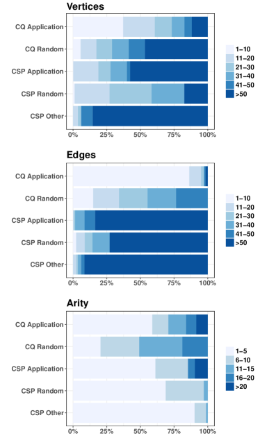
Figure 1. Hypergraph Sizes

Table 1. Overview of benchmark instances

	Benchmark	No. instances	$\mathit{hw}\geq 2$
CQs	SPARQL(Bonifati et al., 2017)	70 (out of 26,157,880)	70
	LUBM(Benedikt et al., 2017; Guo et al., 2005)	14	2
	iBench(Benedikt et al., 2017; Arocena et al., 2015)	40	0
	Doctors(Benedikt et al., 2017; Geerts et al., 2014)	14	0
	Deep(Benedikt et al., 2017)	41	0
	JOB (IMDB) (Leis et al., 2017)	33	7
	TPC-H (Benedikt, 2017; Transaction Processing Performance Council (TPC), 2014)	33	1
	SQLShare (Jain et al., 2016)	290 (out of 15,170)	1
	Random (Pottinger and Halevy, 2001)	500	464
CSPs	Application (Audemard et al., 2016)	1,090	1,090
	Random (Audemard et al., 2016)	863	863
	Other (Gottlob and Samer, 2008; Berg et al., 2017)	82	82
	Total:	3,070	2,580

Hypergraph benchmark. Our benchmark contains 3,070 hypergraphs, which have been converted from CQs and CSPs collected from various sources. Out of these 3,070 hypergraphs, 2,918 hypergraphs have never been used in a hypertree width analysis before. The hypertree width of 70 CQs and of 82 CSPs has been analysed in (Gottlob and Samer, 2008), (Berg et al., 2017), and/or (Bonifati et al., 2017). An overview of all instances of CQs and CSPs is given in Table 1. They have been collected from various publically available benchmarks and repositories of CQs and CSPs. In the first column, the names of each collection of CQs and CSPs are given together with references where they were first published. In the second column we display the number of hypergraphs extracted from each collection. The $\mathit{hw}$ of the CQs and CSPs in our benchmark will be discussed in detail in Section 4. To get a first feeling of the $\mathit{hw}$ of the various sources, we mention the number of cyclic hypergraphs (i.e., those with $\mathit{hw}\geq 2$) in the last column. When gathering the CQs, we proceeded as follows: of the huge benchmark reported in (Bonifati et al., 2017), we have only included CQs, which were detected as having $\mathit{hw}\geq 2$ in (Bonifati et al., 2017). Of the big repository reported in (Jain et al., 2016), we have included those CQs, which are not trivially acyclic (i.e., they have at least 3 atoms). Of all the small collections of queries, we have included all.

Below, we describe the different benchmarks in detail:

$\bullet$  CQs: Our benchmark contains 535 CQs from four main sources (Benedikt, 2017; Benedikt et al., 2017; Bonifati et al., 2017; Jain et al., 2016) and a set of 500 randomly generated queries using the query generator of (Pottinger and Halevy, 2001). In the sequel, we shall refer to the former queries as CQ Application, and to the latter as CQ Random. The CQs analysed in (Bonifati et al., 2017) constitute by far the biggest repository of CQs – namely 26,157,880 CQs stemming from SPARQL queries. The queries come from real-users of SPARQL endpoints and their hypertree width was already determined in (Bonifati et al., 2017). Almost all of these CQs were shown to be acyclic. Our analysis comprises 70 CQs from (Bonifati et al., 2017), which (apart from few exceptions) are essentially the ones in (Bonifati et al., 2017) with $\mathit{hw}\geq 2$. In particular, we have analysed all 8 CQs with highest $\mathit{hw}$ among the CQs analysed in (Bonifati et al., 2017) (namely, $\mathit{hw}=3$).

The LUBM (Guo et al., 2005), iBench (Arocena et al., 2015), Doctors (Geerts et al., 2014), and Deep scenarios have been recently used to evaluate the performance of chase-based systems (Benedikt et al., 2017). Their queries were especially tailored towards the evaluation of query answering tasks of such systems. Note that the LUBM benchmark (Guo et al., 2005) is a widely used standard benchmark for the evaluation of Semantic Web repositories. Its queries are designed to measure the performance of those repositories over large datasets. Strictly speaking, the iBench is a tool for generating schemas, constraints, and mappings for data integration tasks. However, in (Benedikt et al., 2017), 40 queries were created for tests with the iBench. We therefore refer to these queries as iBench-CQs here. In summary, we have incorporated all queries that were either contained in the original benchmarks or created/adapted for the tests in (Benedikt et al., 2017).

The goal of the Join Order Benchmark (JOB) (Leis et al., 2017) was to evaluate the impact of a good join order on the performance of query evaluation in standard RDBMS. Those queries were formulated over the real-world dataset Internet Movie Database (IMDB). All of the queries have between 3 and 16 joins. Clearly, as the goal was to measure the impact of a good join order, those 33 queries are of higher complexity, hence 7 out of the 33 queries have $\mathit{hw}\geq 2$.

The 33 TPC-H queries in our benchmark are taken from the GitHub repository originally provided by Michael Benedikt and Efthymia Tsamoura (Benedikt, 2017) for the work on [12]. Out of the 33 CQs based on the TPC-H benchmark (Transaction Processing Performance Council (TPC), 2014), 13 queries were handcrafted and 20 randomly generated. The TPC-H benchmark has been widely used to assess multiple aspects of the capabilities of RDBMS to process queries. They reflect common workloads in decision support systems and were chosen to have broad industry-wide relevance.

From SQLShare (Jain et al., 2016), a multi-year SQL-as-a-service experiment with a large set of real-world queries, we extracted 15,170 queries by considering all CQs (in particular, no nested SELECTs). After eliminating trivial queries (i.e., queries with $\leq 2$ atoms, whose acyclicity is immediate) and duplicates, we ended up with 290 queries.

The random queries were generated with a tool that stems from the work on query answering using views in (Pottinger and Halevy, 2001). The query generator allows 3 options: chain/star/random queries. Since the former two types are trivially acyclic, we only used the third option. Here it is possible to supply several parameters for the size of the generated queries. In terms of the resulting hypergraphs, one can thus fix the number of vertices, number of edges and arity. We have generated 500 CQs with 5 – 100 vertices, 3 – 50 edges and arities from 3 to 20. These values correspond to the values observed for the CQ Application hypergraphs. However, even though these size values have been chosen similarly, the structural properties of the hypergraphs in two groups CQ Application and CQ Random differ significantly, as will become clear from our analysis in Section 4.

$\bullet$  CSPs: In total, our benchmark currently contains 2,035 hypergraphs from CSP instances, out of which 1,953 instances were obtained from xcsp.org (see also (Audemard et al., 2016)). We have selected all CSP instances from xcsp.org with less than 100 constraints such that all constraints are extensional. These instances are divided into CSPs from concrete applications, called CSP Application in the sequel (1,090 instances), and randomly generated CSPs, called CSP Random below (863 instances). In addition, we have included 82 CSP instances from previous hypertree width analyses provided at https://www.dbai.tuwien.ac.at/proj/hypertree/; all of these stem from industrial applications and/or further CSP benchmarks. We refer to these instances as other CSPs.

Our HyperBench benchmark consists of these instances converted to hypergraphs. In Figure 1, we show the number of vertices, the number of edges and the arity (i.e., the maximum size of the edges) as three important metrics of the size of each hypergraph. The smallest are those coming from CQ Application (at most 10 edges), while the hypergraphs coming from CSPs can be significantly larger (up to 2993 edges). Although some hypergraphs are very big, more than 50% of all hypergraphs have maximum arity less than 5. In Figure 1 we can easily compare the different types of hypergraphs, e.g. hypergraphs of arity greater than 20 only exist in the CSP Application class; the other CSPs class contains the highest portion of hypergraphs with a big number of vertices and edges, etc.

The hypergraphs and the results of their analysis can be accessed through our web tool, available at http://hyperbench.dbai.tuwien.ac.at.

4. First Empirical Analysis

In this section, we present first empirical results obtained with the HyperBench benchmark. On the one hand, we want to get an overview of the hypertree width of the various types of hypergraphs in our benchmark (cf. Goal 2 in Section 1). On the other hand, we want to find out how realistic the restriction to low values for certain hypergraph invariants is (cf. Goal 3 stated in Section 1).

Hypergraph Properties. In (Fischl et al., 2017, [n. d.]), several invariants of hypergraphs were used to make the Check(GHD, $k$) and Check(FHD, $k$) problems tractable or, at least, easier to approximate. We thus investigate the following properties (cf. Definitions 2.4 – 2.7):

• Deg: the degree of the underlying hypergraph

• BIP: the intersection width

• $c$-BMIP: the $c$-multi-intersection width for $c\in\{3,4\}$

• VC-dim: the VC-dimension

Table 2. Hypergraph properties of all benchmark instances

CQ Application
$i$	Deg	BIP	3-BMIP	4-BMIP	VC-dim
0	0	0	118	173	10
1	2	421	348	302	393
2	176	85	59	50	132
3	137	7	5	5	0
4	87	5	5	5	0
5	35	17	0	0	0
6	98	0	0	0	0

CQ Random
$i$	Deg	BIP	3-BMIP	4-BMIP	VC-dim
0	0	1	16	49	0
1	1	17	77	125	20
2	15	53	90	120	133
3	38	62	103	74	240
4	31	63	62	42	106
5	33	71	47	28	1
6	382	233	105	62	0

CSP Application & Other
$i$	Deg	BIP	3-BMIP	4-BMIP	VC-dim
0	0	0	597	603	0
1	0	1037	495	525	0
2	597	95	57	23	1115
3	6	29	21	21	52
4	20	10	2	0	0
5	6	0	0	0	0
$>$5	543	1	0	0	0

CSP Random
$i$	Deg	BIP	3-BMIP	4-BMIP	VC-dim
0	0	0	0	0	0
1	0	200	200	238	0
2	0	224	312	407	220
3	0	76	147	95	515
4	12	181	161	97	57
5	8	99	14	1	71
$>$5	843	83	29	25	0

The results obtained from computing Deg, BIP, $3$-BMIP, $4$-BMIP, and VC-dim for the hypergraphs in the HyperBench benchmark are shown in Table 2.

Table 2 has to be read as follows: In the first column, we distinguish different values of the various hypergraph metrics. In the columns labelled “Deg“, “BIP“, etc., we indicate for how many instances each metric has a particular value. For instance, by the last row in the second column, only 98 non-random CQs have degree $>5$. Actually, for most CQs, the degree is less than 10. Moreover, for the BMIP, already with intersections of 3 edges, we get $\mbox{\it$3$-miwidth($H$)}\leq 2$ for almost all non-random CQs. Also the VC-dimension is at most 2.

For CSPs, all properties may have higher values. However, we note a significant difference between randomly generated CSPs and the rest: For hypergraphs in the groups CSP Application and CSP Other, 543 (46%) hypergraphs have a high degree ($>$5), but nearly all instances have BIP or BMIP of less than 3. And most instances have a VC-dimension of at most 2. In contrast, nearly all random instances have a significantly higher degree (843 out of 863 instances with a degree $>$5). Nevertheless, many instances have small BIP and BMIP. For nearly all hypergraphs (838 out of 863) we have $\mbox{\it$4$-miwidth($H$)}\leq 4$. For 5 instances the computation of the VC-dimension timed out. For all others, the VC-dimension is $\leq 5$ for random CSPs. Clearly, as seen in Table 2, the random CQs resemble the random CSPs a lot more than the CQ and CSP Application instances. For example, random CQs have similar to random CSPs high degree (382 (76%) with degree $>5$), higher BIP and BMIP. Nevertheless, similar to random CSPs, the values for BIP and BMIP are still small for many random CQ instances.

To conclude, for the proposed properties, in particular BIP/BMIP and VC-dimension, most hypergraphs in our benchmark (even for non-random CQs and CSPs) indeed have low values.

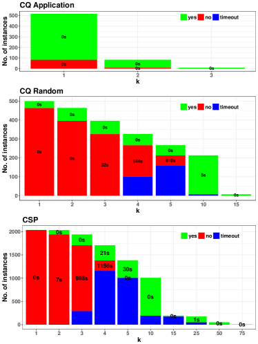
Figure 2. HW analysis (labels are average runtimes in s)

Hypertree Width. We have systematically applied the $\mathit{hw}$-computation from (Gottlob and Samer, 2008) to all hypergraphs in the benchmark. The results are summarized in Figure 2. In our experiments, we proceeded as follows. We distinguish between CQ Application, CQ Random, and all three groups of CSPs taken together. For every hypergraph $H$, we first tried to solve the Check(HD, $k$) problem for $k=1$. In case of CQ Application, we thus got 454 yes-answers and 81 no-answers. The number in each bar indicates the average runtime to find these yes- and no-instances, respectively. Here, the average runtime was “0” (i.e., less than 1 second) in both cases. For CQ Random we got 36 yes- and 464 no-instances with an average runtime below 1 second. For all CSP-instances, we only got no-answers.

In the second round, we tried to solve the Check(HD, $k$) problem for $k=2$ for all hypergraphs that yielded a no-answer for $k=1$. Now the picture is a bit more diverse: 73 of the remaining 81 CQs from CQ Application yielded a yes-answer in less than 1 second. For the hypergraphs stemming from CQ Random (resp. CSPs), only 68 (resp. 95) instances yielded a yes-answer (in less than 1 second on average), while 396 (resp. 1932) instances yielded a no-answer in less than 7 seconds on average and 8 CSP instances led to a timeout (i.e., the program did not terminate within 3,600 seconds).

This procedure is iterated by incrementing $k$ and running the $\mathit{hw}$-computation for all instances, that either yielded a no-answer or a timeout in the previous round. For instance, for queries from CQ Application, one further round is needed after the second round. In other words, we confirm the observation of low $\mathit{hw}$, which was already made for CQs of arity $\leq 3$ in (Bonifati et al., 2017; Picalausa and Vansummeren, 2011). For the hypergraphs stemming from CQ Random (resp. CSPs), 396 (resp. 1940 )instances are left in the third round, of which 70 (resp. 232) yield a yes-answer in less than 1 second on average, 326 (resp. 1415) instances yield a no-answer in 32 (resp. 988) seconds on average and no (resp. 293) instances yield a timeout. Note that, as we increase $k$, the average runtime and the percentage of timeouts first increase up to a certain point and then they decrease. This is due to the fact that, as we increase $k$, the number of combinations of edges to be considered in each $\lambda$-label (i.e., the function $\lambda_{u}$ at each node $u$ of the decomposition) increases. In principle, we have to test $\mathcal{O}(n^{k})$ combinations, where $n$ is the number of edges. However, if $k$ increases beyond a certain point, then it gets easier to “guess” a $\lambda$-label since an increasing portion of the $\mathcal{O}(n^{k})$ possible combinations leads to a solution (i.e., an HD of desired width).

To answer the question in Goal 2, it is indeed the case that for a big number of instances, the hypertree width is small enough to allow for efficient evaluation of CQs or CSPs: all instances of non-random CQs have $\mathit{hw}\leq 3$ no matter whether their arity is bounded by 3 (as in case of SPARQL queries) or not; and a large portion (at least 1027, i.e., ca. 50%) of all 2035 CSP instances have $\mathit{hw}\leq 5$. In total, including random CQs, 1,849 (60%) out of 3,070 instances have $\mathit{hw}\leq 5$, for which we could determine the exact hypertree width for 1,453 instances; the others may even have lower $\mathit{hw}$.

Correlation Analysis. Finally, we have analysed the pairwise correlation between all properties. Of course, the different intersection widths (BIP, 3-BMIP, 4-BMIP) are highly correlated. Other than that, we only observe quite a high correlation of the arity with the number of vertices and the hypertree width and of the number of vertices with the arity and the hypertree width. Clearly, the correlation between arity and hypertree width is mainly due to the CSP instances and the random CQs since, for non-random CQs, the $\mathit{hw}$ never increases beyond $3$, independently of the arity.

A graphical presentation of all pairwise correlations is given in Figure 3. Here, large, dark circles indicate a high correlation, while small, light circles stand for low correlation. Blue circles indicate a positive correlation while red circles stand for a negative correlation. In (Fischl et al., [n. d.]), we have argued that Deg, BIP, 3-BMIP, 4-BMIP and VC-dim are non-trivial restrictions to achieve tractability. It is interesting to note that, according to the correlations shown in Figure 3, these properties have almost no impact on the hypertree width of our hypergraphs. This underlines the usefulness of these restrictions in the sense that (a) they make the GHD computation and FHD approximation easier (Fischl et al., [n. d.]) but (b) low values of degree, (multi-)intersection-width, or VC-dimension do not pre-determine low values of the widths.

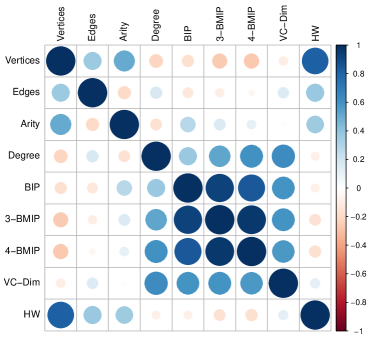
Figure 3. Correlation analysis.

5. GHW Computation

In this section, we report on new algorithms and implementations to solve the Check(GHD, $k$) problem and on new empirical results.

Background. In (Fischl et al., [n. d.]), it is shown that the Check(GHD, $k$) problem becomes tractable for fixed $k\geq 1$, if we restrict ourselves to a class of hypergraphs enjoying the BIP. As our first empirical analysis with the HyperBench has shown (see Section 4), it is indeed realistic to assume that the intersection width of a given hypergraph is small. We have therefore extended the $\mathit{hw}$-computation from (Gottlob and Samer, 2008) by an implementation of the Check(GHD, $k$) algorithm from (Fischl et al., [n. d.]), which will be referred to as the “$\mathit{ghw}$-algorithm” in the sequel. This algorithm is parameterized, so to speak, by two integers: $k$ (the desired width of a GHD) and $i$ (the intersection width of $H$).

The key idea of the $\mathit{ghw}$-algorithm is to add a polynomial-time computable set $f(H,k)$ of subedges of edges in $E(H)$ to the hypergraph $H$, such that $\mathit{ghw}(H)=k$ iff $\mathit{hw}(H^{\prime})=k$ with $H=(V(H),E(H))$ and $H^{\prime}=(V(H),E(H)\cup f(H,k))$. Tractability of Check(GHD, $k$) follows immediately from the tractability of the Check(HD, $k$) problem. The set $f(H,k)$ is defined as

$$f(H,k)=\bigcup_{e\in E(H)}\Big{(}{\bigcup_{e_{1},\ldots,e_{j}\in(E(H)\setminus\{e\}),\,j\leq k}}2^{(e\cap(e_{1}\cup\cdots\cup e_{j}))}\Big{)},$$

i.e., $f(H,k)$ contains all subsets of intersections of edges $e\in E(H)$ with unions of $\leq k$ edges of $H$ different from $e$. By the BIP, the intersection $e\cap(e_{1}\cup\cdots\cup e_{j})$ has at most $i\cdot k$ elements. Hence, for fixed constants $i$ and $k$, $|f(H,k)|$ is polynomially bounded.

“Global” implementation. In a straightforward implementation of this algorithm, we compute $f(H,k)$ and from this $H^{\prime}$ and call the $\mathit{hw}$-computation from (Gottlob and Samer, 2008) for the Check(HD, $k$) problem as a “black box”. A coarse-grained overview of the results is given in Table 3 in the column labelled as ‘GlobalBIP”. We call this implementation of the $\mathit{ghw}$ algorithm of (Fischl et al., [n. d.]) “global” to indicate that the set $f(H,k)$ is computed “globally”, once and for all, for the entire hypergraph. We have run the program on each hypergraph from the HyperBench up to hypertree width $6$, trying to get a smaller $\mathit{ghw}$ than $\mathit{hw}$. We have thus run the $\mathit{ghw}$-algorithm with the following parameters: for all hypergraphs $H$ with $\mathit{hw}(H)=k$ (or $\mathit{hw}\leq k$ and, due to timeouts, we do not know if $\mathit{hw}\leq k-1$ holds), where $k\in\{3,4,5,6\}$, try to solve the Check(GHD, $k-1$) problem. In other words, we just tried to improve the width by 1. Clearly, for $\mathit{hw}(H)\in\{1,2\}$, no improvement is possible since, in this case, $\mathit{hw}(H)=\mathit{ghw}(H)$ holds.

In Table 3, we report on the number of “successful” attempts to solve the Check(GHD, $k-1$) problem for hypergraphs with $\mathit{hw}=k$. Here “successful” means that the program terminated within 1 hour. For instance, for the 310 hypergraphs with $\mathit{hw}=3$ in the HyperBench, the “global” computation terminated in 128 cases (i.e., 41%) when trying to solve Check(GHD, $2$). The average runtime of these “successful” runs was 537 seconds. For the 386 hypergraphs with $\mathit{hw}=4$, the “global” computation terminated in 137 cases (i.e., 35%) with average runtime 2809 when trying to solve the Check(GHD, $3$) problem. For the 886 hypergraphs with $\mathit{hw}\in\{5,6\}$, the “global” computation only terminated in 13 cases (i.e., 1.4%). Overall, it turns out that the set $f(H,k)$ may be very big (even though it is polynomial if $k$ and $i$ are constants). Hence, $H^{\prime}$ can become considerably bigger than $H$. This explains the frequent timeouts in the GlobalBIP column in Table 3.

Table 3. Comparison of GHW algorithms w. avg. runtime (s)

$\mathit{hw}\rightarrow$		GlobalBIP		LocalBIP		BalSep
$\mathit{ghw}$	total	yes	no	yes	no	yes	no
$3\rightarrow 2$	310	-	128 (537)	-	195 (162)	-	307 (12)
$4\rightarrow 3$	386	-	137 (2809)	-	54 (2606)	-	249 (54)
$5\rightarrow 4$	427	-	-	-	-	-	148 (13)
$6\rightarrow 5$	459	13 (162)	-	13 (60)	-	-	180 (288)

“Local” implementation. Looking for ways to improve the $\mathit{ghw}$-algorithm, we closely inspect the role played by the set $f(H,k)$ in the tractability proof in (Fischl et al., [n. d.]). The definition of this set is motivated by the problem that, in the top down construction of a GHD, we may want to choose at some node $u$ the bag $B_{u}$ such that $x\not\in B_{u}$ for some variable $x\in B(\lambda_{u})\cap V(T_{u})$. This violates condition (4) of Definition 2.2 (the “special condition”) and is therefore forbidden in an HD. In particular, there exists an edge $e$ with $x\in e$ and $\lambda_{u}(e)=1$. The crux of the $\mathit{ghw}$-algorithm in (Fischl et al., [n. d.]) is that for every such “missing” variable $x$, the set $f(H,k)$ contains a subedge $e^{\prime}\subseteq e$ with $x\not\in e^{\prime}$. Hence, replacing $e$ by $e^{\prime}$ in $\lambda_{u}$ (i.e., setting $\lambda_{u}(e)=0$, $\lambda_{u}(e^{\prime})=1$ and leaving $\lambda_{u}$ unchanged elsewhere) eliminates the special condition violation. By the connectedness condition, it suffices to consider the intersections of $e$ with unions of edges that may possibly occur in bags of $T_{u}$ rather than with arbitrary edges in $E(H)$. In other words, for each node $u$ in the decomposition, we may restrict $f(H,k)$ to an appropriate subset $f_{u}(H,k)\subseteq f(H,k)$.

The results obtained with this enhanced version of the $\mathit{ghw}$-computation are shown in Table 3 in the column labelled “LocalBIP”. We call this implementation of $\mathit{ghw}$-computation “local” because the set $f_{u}(H,k)$ of subedges of $H$ to be added to the hypergraph is computed separately for each node $u$ of the decomposition. Recall that in this table, the “successful” calls of the program are recorded. Interestingly, for the hypergraphs with $\mathit{hw}=3$, the “local” computation performs significantly better (namely 63% solved with average runtime 162 seconds rather than 41% with average runtime 537 seconds). In contrast, for the hypergraphs with $\mathit{hw}=4$, the “global” computation is significantly more successful. For $\mathit{hw}\in\{5,6\}$, the “global” and “local” computations are equally bad. A possible explanation for the reverse behaviour of “global” and “local” computation in case of $\mathit{hw}=3$ as opposed to $\mathit{hw}=4$ is that the restriction of the “global” set $f(H,k)$ of subedges to the “local” set $f_{u}(H,k)$ at each node $u$ seems to be quite effective for the hypergraphs with $\mathit{hw}=3$. In contrast, the additional cost of having to compute $f_{u}(H,k)$ at each node $u$ becomes counter-productive, when the set of subedges thus eliminated is not significant. It is interesting to note that the sets of solved instances of the global computation and the local computation are incomparable, i.e., in some cases one method is better, while in other cases the other method is better.

ALGORITHM Find_GHD_via_balancedSeparators // high-level description Input:    hypergraph $H^{\prime}$, integer $k\geq 0$. Output: a GHD $\left<T,B_{u},\lambda_{u}\right>$ of width $\leq k$ if exists,             “Reject”, otherwise. Procedure Find_GHD ($H$: Hypergraph, $\mathit{Sp}$: Set of special edges) begin 1. Base Case: if there are only special edges left and $|\mathit{Sp}|\leq 2$ then stop and return a GHD with one node for each special edge. 2. Find a balanced separator: for all functions $\lambda\colon E(H^{\prime})\rightarrow\{0,1\}$ check if $\lambda_{u}$ is a balanced separator for $H$; if none is found then return Reject. 3. Split $H$ into connected components $C_{1},\dots,C_{\ell}$ w.r.t. $\lambda_{u}$: $C_{i}\subseteq V(H)\setminus B(\lambda_{u})$ for every $i$ and $C_{i}$ is connected in $H$ and each $C_{i}$ is maximal with this property. 4. Build the pair $\left<H_{i},\mathit{Sp}_{i}\right>$ (the subhypergraph based on $C_{i}$ and the special edges in $C_{i}$) for each connected component $C_{i}$; add $B(\lambda_{u})$ as one more special edge to each set $\mathit{Sp}_{i}$. 5. Call Find_GHD($H_{i}$, $\mathit{Sp}_{i}$) for each pair $\left<H_{i},\mathit{Sp}_{i}\right>$; each successful call returns a GHD $T_{i}$ for $H_{i}$ if one call returns Reject then return Reject. 6. Create and return a new GHD for $H$ having $\lambda_{u}$ as root: each $T_{i}$ has one leaf node labelled $B(\lambda_{u})$; the new GHD is obtained by gluing together all subtrees $T_{i}$ at the node with label $B(\lambda_{u})$. end begin (* Main *) return Find_GHD ($H^{\prime}$, $\emptyset$); end

Figure 4. Recursive GHD-algorithm via balanced separators

New alternative approach: “balanced separators”. We now propose a completely new approach, based on so-called “balanced separators”. The latter are a familiar concept in graph theory (Feige and Mahdian, 2006; Schild and Sommer, 2015) – denoting a set $S$ of vertices of a graph $G$, such that the subgraph $G^{\prime}$ induced by $V(G)\setminus S$ has no connected component larger than some given size, e.g., $\alpha\cdot|V|$ for some given $\alpha\in(0,1)$. In our setting, we may consider the label $\lambda_{u}$ at some node $u$ in a GHD as separator in the sense that we can consider connected components of the subhypergraph $H^{\prime}$ of $H$ induced by $V(H)\setminus B_{u}$. Clearly, in a GHD, we may consider any node as the root. So suppose that $u$ is the root of some GHD. Moreover, as is shown in (Fischl et al., [n. d.]) in the proof of tractability of Check(GHD, $k$) in case of the BIP, we may choose $\lambda_{u}$ such that $B(\lambda_{u})=B_{u}$ if the subedges in $f(H,k)$ have been added to the hypergraph.

By the HD-algorithm from (Gottlob et al., 2002), we know that an HD of $H^{\prime}$ (and, hence, a GHD of $H$) can be constructed in such a way that every subtree rooted at a child node $u_{i}$ of $u$ contains only one connected component $C_{i}$ of the subhypergraph of $H^{\prime}$ induced by $V(H)\setminus B_{u}$. For our purposes, it is convenient to define the size of a component $C_{i}$ as the number of edges that have to be covered at some node in the subtree rooted at $u_{i}$ in the GHD. We thus call a separator $\lambda_{u}$ “balanced”, if the size of each component $C_{i}$ is at most $|E(H^{\prime})|/2$. The following observation is immediate:

Proposition 5.1.

In every GHD, there exists a node $u$ (which we may choose as the root) such that $\lambda_{u}$ is a balanced separator.

This property allows us to design the algorithm sketched in Figure 4 to compute a GHD of $H^{\prime}$. Actually, as will become clear below, we assume that the input to this recursive algorithm consists of a hypergraph plus a set $\mathit{Sp}$ of “special edges” and we request that the GHD to be constructed contains “special nodes”, which (a) have to be leaf nodes in the decomposition and (b) the $\lambda$-label of such a leaf node consists of a single special edge only. Each special edge contains the set of vertices $B_{u}$ of some balanced separator $\lambda_{u}$ further up in the hierarchy of recursive calls of the decomposition algorithm. The special edges are propagated to the recursive calls for subhypergraphs in order to determine how to assemble the overall GHD from the GHDs of the subhypergraphs. This will become clearer in the proof sketch of Theorem 5.2.

Theorem 5.2.

Let $H$ be a hypergraph, let $k\geq 1$, and let $H^{\prime}$ be obtained from $H$ by adding the subedges in $f(H,k)$ to $E(H)$. Then the algorithm Find_GHD_via_balancedSeparators given in Figure 4 outputs a GHD of width $\leq k$ if one exists and rejects otherwise.

Proof Sketch.

Steps 1 –5 of the algorithm in Figure 4 essentially correspond to the computation of $\lambda_{u}$ and $B_{u}$ for the root node $u$ in the HD-computation of (Gottlob et al., 2002). The most significant modifications here are due to the handling of “special edges” in parameter $Sp$. A crucial property of the construction in (Gottlob et al., 2002) and also of our construction here is that each subtree below node $u$ in the decomposition only contains vertices from a single connected component $C_{i}$ w.r.t. $V(H)\setminus B_{u}$ (see Steps 3 and 4). Since the special edges come from such bags $B_{u}$, special edges can never be used as separators in recursive calls below. Hence, the base case (in Step 1) is reached for $E(H)=\emptyset$ and $|Sp|\leq 2$. Indeed, $|Sp|\geq 3$ cannot occur because then one of the special edges would have to be a separator of the remaining special edges. Moreover, we can exclude special edges from the search for a balanced separator (in Step 2).

The correctness of assembling a GHD (in Step 6) from the results of the recursive calls can be shown by structural induction on the tree structure of a GHD: suppose that the recursive calls in the algorithm for each hypergraph $H_{i}$ with set $\mathit{Sp}_{i}$ of special edges are correct, i.e., they yield for each hypergraph $H_{i}$ a GHD ${\cal D}_{i}$ such that each special edge $s$ in $\mathit{Sp}_{i}$ is indeed covered by a leaf node in ${\cal D}_{i}$ whose $\lambda$-label consists of $s$ only. In particular, since $s=B(\lambda_{u})$ is a special edge contained in $\mathit{Sp}_{i}$ for each $i$, there exists a leaf node $t_{i}$ in ${\cal D}_{i}$ with $\lambda_{t_{i}}=\{s\}$. In a GHD, any node can be taken as the root. We thus choose $t_{i}$ as the root node in each GHD ${\cal D}_{i}$. By construction, we have $B_{u}=B_{t_{1}}=\dots=B_{t_{\ell}}$. Moreover, any two subhypergraphs $H_{i}$, $H_{j}$ contain the vertices from two different connected components. Hence, apart from the vertices contained in the special edge $s$, any two GHDs ${\cal D}_{i}$, ${\cal D}_{j}$ with $i\neq j$ have no vertices in common. We can therefore construct a GHD ${\cal D}$ of $H^{\prime}$ by deleting the root node $t_{i}$ from each GHD ${\cal D}_{i}$ and by appending the child nodes of each $t_{i}$ directly as child nodes of $u$. Clearly, the connectedness condition is satisfied in the resulting decomposition. ∎

If we look at the number of solved instances in Table 3, we see that the recursive algorithm via balanced separators (reported in the last column labelled BalSep) has the least number of timeouts due to the fast identification of negative instances (i.e., those with no-answer), where it often detects quite fast that a given hypergraph does not have a balanced separator of desired width. As $k$ increases, the performance of the balanced separators approach deteriorates. This is due to $k$ in the exponent of the running time of our algorithm, i.e. we need to check for each of the possible $\mathcal{O}(n^{k+1})$ combinations of $\leq k$ edges if it constitutes a balanced separator.

Table 4. GHW of instances with average runtime in s

$\mathit{hw}\rightarrow\mathit{ghw}$	yes	no	timeout
$3\rightarrow 2$	0	309 (10)	1
$4\rightarrow 3$	0	262 (57)	124
$5\rightarrow 4$	0	148 (13)	279
$6\rightarrow 5$	18 (129)	180 (288)	261

Empirical results. We now look at Table 4, where we report for all hypergraphs with $\mathit{hw}\leq k$ and $k\in\{3,4,5,6\}$, whether $\mathit{ghw}\leq k-1$ could be verified. To this end, we run our three algorithms (“global”, “local”, and “balanced separators”) in parallel and stop the computation, as soon as one terminates (with answer “yes” or “no”). The number in parentheses refers to the average runtime needed by the fastest of the three algorithms in each case. A timeout occurs if none of the three algorithms terminates within 3,600 seconds. It is interesting to note that in the vast majority of cases, no improvement of the width is possible when we switch from $\mathit{hw}$ to $\mathit{ghw}$: in 98% of the solved cases and 57% of all instances with $\mathit{hw}\leq 6$, $\mathit{hw}$ and $\mathit{ghw}$ have identical values. Actually, we think that the high percentage of the solved cases gives a more realistic picture than the percentage of all cases for the following reason: our algorithms (in particular, the “global” and “local” computations) need particularly long time for negative instances. This is due to the fact that in a negative case, “all” possible choices of $\lambda$-labels for a node $u$ in the GHD have to be tested before we can be sure that no GHD of $H$ (or, equivalently, no HD of $H^{\prime}$) of desired width exists. Hence, it seems plausible that the timeouts are mainly due to negative instances. This also explains why our new GHD algorithm in Figure 4, which is particularly well suited for negative instances, has the least number of timeouts.

We conclude this section with a final observation: in Figure 2, we had many cases, for which only some upper bound $k$ on the $\mathit{hw}$ could be determined, namely those cases, where the attempt to solve Check(HD, $k$) yields a yes-answer and the attempt to solve Check(HD, $k-1$) gives a timeout. In several such cases, we could get (with the balanced separator approach) a no-answer for the Check(GHD, $k-1$) problem, which implicitly gives a no-answer for the problem Check(HD, $k-1$). In this way, the alternative approach to the $\mathit{ghw}$-computation is also profitable for the $\mathit{hw}$-computation: for 827 instances with $\mathit{hw}\leq 6$, we were not able to determine the exact hypertree width. Using our new $\mathit{ghw}$-algorithm, we closed this gap for 297 instances; for these instances $\mathit{hw}=\mathit{ghw}$ holds.

To sum up, we now have a total of 1,778 (58%) instances for which we determined the exact hypertree width and a total of 1,406 instances (46%) for which we determined the exact generalized hypertree width. Out of these, 1,390 instances had identical values for $\mathit{hw}$ and $\mathit{ghw}$. In 16 cases, we found an improvement of the width by 1 when moving from $\mathit{hw}$ to $\mathit{ghw}$, namely from $\mathit{hw}=6$ to $\mathit{ghw}=5$. In 2 further cases, we could show $\mathit{hw}\leq 6$ and $\mathit{ghw}\leq 5$, but the attempt to check $\mathit{hw}=5$ or $\mathit{ghw}=4$ led to a timeout. Hence, in response to Goal 6, $\mathit{hw}$ is equal to $\mathit{ghw}$ in 45% of the cases if we consider all instances and in 60% of the cases (1,390 of 2,308) with small width ($\mathit{hw}\leq 6$). However, if we consider the fully solved cases (i.e., where we have the precise value of $\mathit{hw}$ and $\mathit{ghw}$), then $\mathit{hw}$ and $\mathit{ghw}$ coincide in 99% of the cases (1,390 of 1,406).

6. Fractionally Improved Decompositions

The algorithms proposed in the literature for computing FHDs are very expensive. For instance, even the algorithm used for the tractability result in (Fischl et al., 2017) for hypergraphs of low degree is problematical since it involves a double-exponential factor in the degree. Therefore, we investigate the potential of a simplified method to compute approximated FHDs. Below, we present two algorithms for such approximated FHD computations – with a trade-off between computational cost and quality of the approximation.

$\bullet$  The simplest way to obtain a fractionally improved (G)HD is to take either a GHD or HD as input and compute a fractionally improved (G)HD. To this end, an algorithm (which we refer to as SimpleImproveHD) visits each node $u$ of a given GHD or HD and computes an optimal fractional edge cover $\gamma_{u}$ for the set $B_{u}$ of vertices. This algorithm is simple and computationally inexpensive, provided that we can start off with a GHD or HD that was computed before. In our case, we simply took the HD resulting from the $\mathit{hw}$-computation reported in Figure 2. Clearly, this approach is rather naive and the dependence on a concrete HD is unsatisfactory. We therefore move to a more sophisticated algorithm described next.

$\bullet$  The algorithm FracImproveHD has as input a hypergraph $H$ and numbers $k,k^{\prime}\geq 1$, where $k$ is an upper bound on the $\mathit{hw}$ and $k^{\prime}$ the desired fractionally improved $\mathit{hw}$. We search for an FHD ${\cal D^{\prime}}$ with ${\cal D^{\prime}}=\mathit{SimpleImproveHD}({\cal D})$ for some HD ${\cal D}$ of $H$ with $\mathit{width}({\cal D})\leq k$ and $\mathit{width}({\cal D^{\prime}})\leq k^{\prime}$. In other words, this algorithm searches for the best fractionally improved HD over all HDs of width $\leq k$. Hence, the result is independent of any concrete HD.

The experimental results with these algorithms for computing fractionally improved HDs are summarized in Table 5 and Table 6.

We have applied these algorithms to all hypergraphs for which $\mathit{hw}\leq k$ with $k\in\{2,3,4,5\}$ is known from Figure 2. The various columns of the Tables 5 and 6 are as follows: the first column (labelled $\mathit{hw}$) refers to the (upper bound on the) $\mathit{hw}$ according to Figure 2. The next 3 columns, labelled $\geq 1$, $[0.5,1)$, and $[0.1,0.5)$ tell us, by how much the width can be improved (if at all) if we compute an FHD by one of the two algorithms. We thus distinguish the 3 cases if, for a hypergraph of $\mathit{hw}\leq k$, we manage to construct an FHD of width $k-c$ for $c\geq 1$, $c\in[0.5,1)$, or $c\in[0.1,0.5)$. The column with label “no” refers to the cases where no improvement at all or at least no improvement by $c\geq 0.1$ was possible. The last column counts the number of timeouts.

For instance, in the first row of Table 5, we see that (with the SimpleImproveHD algorithm and starting from the HD obtained by the $\mathit{hw}$-computation of Figure 2) out of 238 hypergraphs with $\mathit{hw}=2$, no improvement was possible in 172 cases. In the remaining 66 cases, an improvement to a width of at most $2-0.5$ was possible in 25 cases and an improvement to $k-c$ with $c\in[0.1,0.5)$ was possible in 41 cases. For the hypergraphs with $\mathit{hw}=3$ in Figure 2, almost half of the hypergraphs (141 out of 310) allowed at least some improvement, in particular, 104 by $c\in[0.5,1)$ and 12 even by at least 1. The improvements achieved for the hypergraphs with $\mathit{hw}\leq 4$ and $\mathit{hw}\leq 5$ are less significant.

Table 5. Instances solved with SimpleImproveHD

$\mathit{hw}$	$\geq 1$	$[0.5,1)$	$[0.1,0.5)$	no	timeout
$2$	$0$	$41$	$25$	$172$	$0$
$3$	$12$	$104$	$25$	$169$	$0$
$4$	$9$	$55$	$11$	$311$	$0$
$5$	$20$	$14$	$11$	$382$	$0$
$6$	$12$	$60$	$80$	$309$	$0$

Table 6. Instances solved with FracImproveHD

$\mathit{hw}$	$\geq 1$	$[0.5,1)$	$[0.1,0.5)$	no	timeout
$2$	0	46	29	160	1
$3$	14	116	21	135	24
$4$	11	81	2	8	284
$5$	18	126	59	2	222
$6$	28	149	95	4	183

The results obtained with our implementation of the FracImproveHD algorithm are displayed in Table 6. We see that the number of hypergraphs which allow for a fractional improvement of the width by at least 0.5 or even by 1 is often bigger than with SimpleImproveHD – in particular in the cases where $k^{\prime}\leq k$ with $k\in\{4,5\}$ holds. In the other cases, the results obtained with the naive SimpleImproveHD algorithm are not much worse than with the more sophisticated FracImproveHD algorithm.

7. Related Work

We distinguish several types of works that are highly relevant to ours. The works most closely related are the descriptions of HD, GHD and FHD algorithms in (Gottlob et al., 2002; Fischl et al., [n. d.]) and the implementation of HD computation by the DetKDecomp program reported in (Gottlob and Samer, 2008). We have extended these works in several ways. Above all, we have incorporated our analysis tool (reported in Sections 3 and 4) and the GHD and FHD computations (reported in Sections 5 and 6) into the DetKDecomp program – resulting in our NewDetKDecomp library, which is openly available on GitHub. For the GHD computation, we have added heuristics to speed up the basic algorithm from (Fischl et al., [n. d.]). Moreover, we have proposed a novel approach via balanced separators, which allowed us to significantly extend the range of instances for which the GHD computation terminates in reasonable time. We have also introduced a new form of decomposition method: the fractionally improved decompositions (see Section 6), which allow for a practical, lightweight form of FHDs.

The second important input to our work comes from the various sources (Arocena et al., 2015; Benedikt, 2017; Benedikt et al., 2017; Berg et al., 2017; Geerts et al., 2014; Gottlob and Samer, 2008; Leis et al., 2015; Jain et al., 2016; Transaction Processing Performance Council (TPC), 2014) which we took our CQs and CSPs from. Note that our main goal was not to add further CQs and/or CSPs to these benchmarks. Instead, we have aimed at taking and combining existing, openly accessible benchmarks of CQs and CSPs, convert them into hypergraphs, which are then thoroughly analysed. Finally, the hypergraphs and the analysis results are made openly accessible again.

The third kind of works highly relevant to ours are previous analyses of CQs and CSPs. To the best of our knowledge, Ghionna et al. (Ghionna et al., 2007) presented the first systematic study of HDs of benchmark CQs from TPC-H. However, Ghionna et al. pursued a research goal different from ours in that they primarily wanted to find out to what extent HDs can actually speed up query evaluation. They achieved very positive results in this respect, which have recently been confirmed by the work of Perelman et al. (Perelman and Ré, 2015), Tu et al. (Tu and Ré, 2015) and Aberger et al. (Aberger et al., 2016a; Aberger et al., 2017) on query evaluation using FHDs. As a side result, Ghionna et al.  also detected that CQs tend to have low hypertree width (a finding which was later confirmed in (Bonifati et al., 2017; Picalausa and Vansummeren, 2011) and also in our study). In a pioneering effort, Bonifati, Martens, and Timm (Bonifati et al., 2017) have recently analysed an unprecedented, massive amount of queries: they investigated 180,653,910 queries from (not openly available) query logs of several popular SPARQL endpoints. After elimination of duplicate queries, there were still 56,164,661 queries left, out of which 26,157,880 queries were in fact CQs. The authors thus significantly extend previous work by Picalausa and Vansummeren (Picalausa and Vansummeren, 2011), who analysed 3,130,177 SPARQL queries posed by humans and software robots at the DBPedia SPARQL endpoint. The focus in (Picalausa and Vansummeren, 2011) is on structural properties of SPARQL queries such as keywords used and variable structure in optional patterns. There is one paragraph devoted to CQs, where it is noted that 99.99% of ca.  2 million CQs considered in (Picalausa and Vansummeren, 2011) are acyclic.

Many of the CQs (over 15 million) analysed in (Bonifati et al., 2017) have arity 2 (here we consider the maximum arity of all atoms in a CQ as the arity of the query), which means that all triples in such a SPARQL query have a constant at the predicate-position. Bonifati et al. made several interesting observations concerning the shape of these graph-like queries. For instance, they detected that exactly one of these queries has $\mathit{tw}=3$, while all others have $\mathit{tw}\leq 2$ (and hence $\mathit{hw}\leq 2$). As far as the CQs of arity 3 are concerned (for CQs expressed as SPARQL queries, this is the maximum arity achievable), among many characteristics, also the hypertree width was computed by using the original DetKDecomp program from (Gottlob and Samer, 2008). Out of 6,959,510 CQs of arity 3, only 86 (i.e. 0.01‰) turned out to have $\mathit{hw}=2$ and 8 queries had $¸\mathit{hw}=3$, while all other CQs of arity 3 are acyclic. Our analysis confirms that, also for non-random CQs of arity $>3$, the hypertree width indeed tends to be low, with the majority of queries being even acyclic.

For the analysis of CSPs, much less work has been done. Although it has been shown that exploiting (hyper-) tree decompositions may significantly improve the performance of CSP solving (Amroun et al., 2016; Habbas et al., 2015; Karakashian et al., 2011; Lalou et al., 2009), a systematic study on the (generalized) hypertree width of CSP instances has only been carried out by few works (Gottlob and Samer, 2008; Lalou et al., 2009; Schafhauser, 2006). To the best of our knowledge, we are the first to analyse the $\mathit{hw}$, $\mathit{ghw}$, and $\mathit{fhw}$ of ca. 2,000 CSP instances, where most of these instances have not been studied in this respect before.

It should be noted that the focus of our work is different from the above mentioned previous works: above all, we wanted to test the practical feasibility of various algorithms for HD, GHD, and FHD computation (including both, previously presented algorithms and new ones developed as part of this work). As far as our repository of hypergraphs (obtained from CQs and CSPs) is concerned, we emphasize open accessibility. Thus, users can analyse their CQs and CSPs (with our implementations of HD, GHD, and FHD algorithms) or they can analyse new decomposition algorithms (with our hypergraphs, which cover quite a broad range of characteristics). In fact, in the recent work on FHD computation via SMT solving (Fichte et al., 2018), the Hyperbench benchmark has already been used for the experimental evaluation. In (Fichte et al., 2018) a novel approach to $\mathit{fhw}$ computation via an efficient encoding of the check-problem for FHDs to SMT (SAT modulo Theory) is presented. The tests were carried out with 2,191 hypergraphs from the initial version of the HyperBench. For all of these hypergraphs we have established at least some upper bound on the $\mathit{fhw}$ either by our $\mathit{hw}$-computation or by one of our new algorithms presented in Sections 5 and 6. In contrast, the exact algorithm in (Fichte et al., 2018) found FHDs only for 1.449 instances (66%). In 852 cases, both our algorithms and the algorithm in (Fichte et al., 2018) found FHDs of the same width; in 560 cases, an FHD of lower width was found in (Fichte et al., 2018). By using the same benchmark for the tests, the results in (Fichte et al., 2018) and ours are comparable and have thus provided valuable input for future improvements of the algorithms by combining the different strengths and weaknesses of the two approaches.

The use of the same benchmark has also allowed us to provide feedback to the authors of (Fichte et al., 2018) for debugging their system: in 9 out of 2,191 cases, the “optimal” value for the $\mathit{fhw}$ computed in [19] was apparently erroneous, since it was higher than the $\mathit{hw}$ found out by our analysis; note that upper bounds on the width are, in general, more reliable than lower bounds since it is easy to verify if a given decomposition indeed has the desired properties, whereas ruling out the existence of a decomposition of a certain width is a complex and error-prone task.

8. Conclusion

In this work, we have presented HyperBench, a new and comprehensive benchmark of hypergraphs derived from CQs and CSPs from various areas, together with the results of extensive empirical analyses with this benchmark.

Lessons learned. The empirical study has brought many insights. Below, we summarize the most important lessons from our studies.

$\bullet$  The finding of (Bonifati et al., 2017; Picalausa and Vansummeren, 2011) that non-random CQs have low hypertree width has been confirmed by our analysis, even if (in contrast to SPARQL queries) the arity of the CQs is not bounded by 3. For random CQs and CSPs, we have detected a correlation between the arity and the hypertree width, although also in this case, the increase of the $\mathit{hw}$ with increased arity is not dramatic.

$\bullet$  In (Fischl et al., [n. d.]), several hypergraph invariants were identified, which make the computation of GHDs and the approximation of FHDs tractable. We have seen that, at least for non-random instances, these invariants indeed have low values.

$\bullet$  The reduction of the $\mathit{ghw}$-computation problem to the $\mathit{hw}$-computation problem in case of low intersection width turned out to be more problematical than the theoretical tractability results from (Fischl et al., [n. d.]) had suggested. Even the improvement by “local” computation of the additional subedges did not help much. However, we were able to improve this significantly by presenting a new algorithm based on “balanced separators”. In particular for negative instances (i.e., those with a no-answer), this approach proved very effective.

$\bullet$  An additional benefit of the new $\mathit{ghw}$-algorithm based on “balanced separators” is that it allowed us to also fill gaps in the $\mathit{hw}$-computation. Indeed, in several cases, we managed to verify $\mathit{hw}\leq k$ for some $k$ but we could not show $\mathit{hw}\not\leq k-1$, due to a timeout for Check(HD, $k-1$). By establishing $\mathit{ghw}\not\leq k-1$ with our new GHD-algorithm, we have implicitly showed $\mathit{hw}\not\leq k-1$. This allowed us to compute the exact $\mathit{hw}$ of many further hypergraphs.

$\bullet$  Most surprisingly, the discrepancy between $\mathit{hw}$ and $\mathit{ghw}$ is much lower than expected. Theoretically, only the upper bound $\mathit{hw}\leq 3\cdot\mathit{ghw}+1$ is known. However, in practice, when considering hypergraphs of $\mathit{hw}\leq 6$, we could show that in 53% of all cases, $\mathit{hw}$ and $\mathit{ghw}$ are simply identical. Moreover, in all cases when one of our implementations of $\mathit{ghw}$-computation terminated on instances with $\mathit{hw}\leq 5$, we got identical values for $\mathit{hw}$ and $\mathit{ghw}$.

Future work. Our empirical study has also given us many hints for future directions of research. We find the following tasks particularly urgent and/or rewarding.

$\bullet$  So far, we have only implemented the $\mathit{ghw}$-computation in case of low intersection width. In (Fischl et al., [n. d.]), tractability of the Check(GHD, $k$) problem was also proved for the more relaxed bounded multi-intersection width. Our empirical results in Figure 6 show that, apart from the random CQs and random CSPs, the 3-multi-intersection is $\leq 2$ in almost all cases. It seems therefore worthwhile to implement and test also the BMIP-algorithm from (Fischl et al., [n. d.]).

$\bullet$  The three approaches for $\mathit{ghw}$-computation presented here turned out to have complementary strengths and weaknesses. This was profitable when running all three algorithms in parallel and taking the result of the first one that terminates (see Table 4). In the future, we also want to implement a more sophisticated combination of the various approaches: for instance, one could try to apply our new “balanced separator” algorithm recursively only down to a certain recursion depth (say depth 2 or 3) to split a big given hypergraph into smaller subhypergraphs and then continue with the “global” or “local” computation from Section 5.

$\bullet$  Our new approach to $\mathit{ghw}$-computation via “balanced separators” proved quite effective in our experiments. However, further theoretical underpinning of this approach is missing. The empirical results obtained for our new GHD algorithm via balanced separators suggest that the number of balanced separators is often drastically smaller than the number of arbitrary separators. We want to determine a realistic upper bound on the number of balanced separators in terms of $n$ (the number of edges) and $k$ (an upper bound on the width). This will then allow us to compute also a realistic upper bound on the runtime of this new algorithm.

$\bullet$  Finally, we want to further extend the HyperBench benchmark and tool in several directions. We will thus incorporate further implementations of decomposition algorithms from the literature such as the GHD- and FHD computation in (Moll et al., 2012) or the polynomial-time FHD computation for hypergraphs of bounded degree in (Fischl et al., 2017). Moreover, we will continue to fill in hypergraphs from further sources of CSPs and CQs. For instance, in (Aberger et al., 2017; Carmeli et al., 2017; Ghionna et al., 2007; Ghionna et al., 2011) a collection of CQs for the experimental evaluations in those papers is mentioned. We will invite the authors to disclose these CQs and incorporate them into the HyperBench benchmark.

$\bullet$  Very recently, a new, huge, publically available query log has been reported in (Malyshev et al., 2018). It contains over 200 million SPARQL queries on Wikidata. In the paper, the anonymisation and publication of the query logs is mentioned as future work. However, on their web site, the authors have meanwhile made these queries available. At first glance, these queries seem to display a similar behaviour as the SPARQL queries collected by Bonifatti et al. (Bonifati et al., 2017): there is a big number of single-atom queries and again, the vast majority of the queries is acyclic. A detailed analysis of the query log in the style of (Bonifati et al., 2017) constitutes an important goal for future research.

Acknowledgements

We would like to thank Angela Bonifati, Wim Martens, and Thomas Timm for sharing most of the hypergraphs with $\mathit{hw}\geq 2$ from their work (Bonifati et al., 2017) and for their effort in anonymising these hypergraphs, which was required by the license restrictions.

Appendix

In this appendix, we present further details of our analyses. First, we will present the web tool to browse and discover the hypergraphs that we have used. In addition, above all, we provide additional figures and tables to allow for a more fine-grained view on the CSP instances. Recall from Section 3 that we are dealing with 3 classes of CSP instance here: CSP Application and CSP Random, which are both taken from xcsp.org (Audemard et al., 2016), and CSP Other, which have already been analysed w.r.t. $\mathit{hw}$ in previous works (Gottlob and Samer, 2008; Berg et al., 2017). Due to lack of space, the main body of the text contains only figures and tables with aggregated values for all CSPs. Below, additional details are provided for each figure and table from the main body by distinguishing the two classes of CQs and three classes of CSPs.

Appendix A Web tool

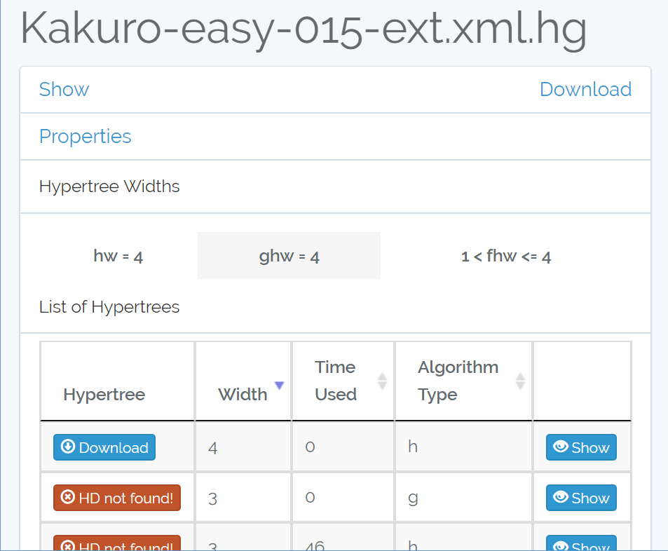
Figure 5. HyperBench web tool: available at
http://hyperbench.dbai.tuwien.ac.at

The hypergraphs in the benchmark and the results of the analyses of these hypergraphs can be accessed via a web tool, which is available at http://hyperbench.dbai.tuwien.ac.at. There we have uploaded 3,070 hypergraphs together with over 5,518 HDs and the output of over 16,585 further algorithm runs, where no HD of desired width was found (either because a lower bound on the width was established or the algorithm timed out). For example, in the screenshot in Figure 5 the results for the CSP instance “Kakuro-easy-015-ext.xml.hg” are displayed. The hypertree width of the instance is calculated according to the list of HDs at the bottom of the screenshot. For this instance we have several algorithm runs, some of which led to a HD, some did not (“HD not found”). With these we were able to pinpoint that $\mathit{hw}=\mathit{ghw}=4$ holds. All instances can be explored in such a way.

Additionally, we allow the user to browse, download and inspect hypergraph categories presented in this work. In the near future, we will also provide a search interface to download instances having specific properties (e.g. $\mathit{hw}<5$ or BIP $<3$, etc.) and to contribute to the benchmark by uploading hypergraphs, which are then analysed and incorporated into our HyperBench benchmark.

Appendix B Further Details for Section 3

Table 7 presents the exact numbers used in Figure 1.

Vertices
	$1-10$	$11-20$	$21-30$	$31-40$	$41-50$	$>50$
CQ Application	199	126	67	51	29	63
CQ Random	28	59	58	62	60	233
CSP Application	2	204	97	133	27	627
CSP Random	10	224	269	210	0	150
CSP Other	0	3	2	0	7	70

Edges
	$1-10$	$11-20$	$21-30$	$31-40$	$41-50$	$>50$
CQ Application	462	47	11	1	6	8
CQ Random	75	96	106	106	117	0
CSP Application	1	5	12	76	85	911
CSP Random	20	55	50	110	0	628
CSP Other	0	2	1	2	2	75

Arities
	$1-5$	$6-10$	$11-15$	$16-20$	$>20$
CQ Application	315	64	70	41	45
CQ Random	102	144	160	94	0
CSP Application	667	263	1	56	103
CSP Random	594	244	25	0	0
CSP Other	74	7	1	0	0

Table 7. Hypergraph Sizes

Appendix C Further Details for Section 4

In Table 2, statistics on several hypergraph invariants were provided, namely degree, intersection width, $c$-multi-intersection width for $c\in\{3,4\}$, and VC-dimension. In Table 8 and Figure 6, additional details are provided by distinguishing the three classes of CSP instances.

CQ Application
$i$	Deg	BIP	3-BMIP	4-BMIP	VC-dim
0	0	0	118	173	10
1	2	421	348	302	393
2	176	85	59	50	132
3	137	7	5	5	0
4	87	5	5	5	0
5	35	17	0	0	0
6	98	0	0	0	0

CQ Random
$i$	Deg	BIP	3-BMIP	4-BMIP	VC-dim
0	0	1	16	49	0
1	1	17	77	125	20
2	15	53	90	120	133
3	38	62	103	74	240
4	31	63	62	42	106
5	33	71	47	28	1
6	382	233	105	62	0

CSP Application
$i$	Deg	BIP	3-BMIP	4-BMIP	VC-dim
0	0	0	596	597	0
1	0	1030	459	486	0
2	596	59	34	7	1064
3	1	0	1	0	26
4	1	0	0	0	0
5	2	0	0	0	0
$>$5	490	1	0	0	0

CSP Random
$i$	Deg	BIP	3-BMIP	4-BMIP	VC-dim
0	0	0	0	0	0
1	0	200	200	238	0
2	0	224	312	407	220
3	0	76	147	95	515
4	12	181	161	97	57
5	8	99	14	1	71
$>$5	843	83	29	25	0

CSP Other
$i$	Deg	BIP	3-BMIP	4-BMIP	VC-dim
0	0	0	1	6	0
1	0	7	36	39	0
2	1	36	23	16	51
3	5	29	20	21	26
4	19	10	2	0	0
5	4	0	0	0	0
$>5$	53	0	0	0	0

Table 8. Hypergraph properties

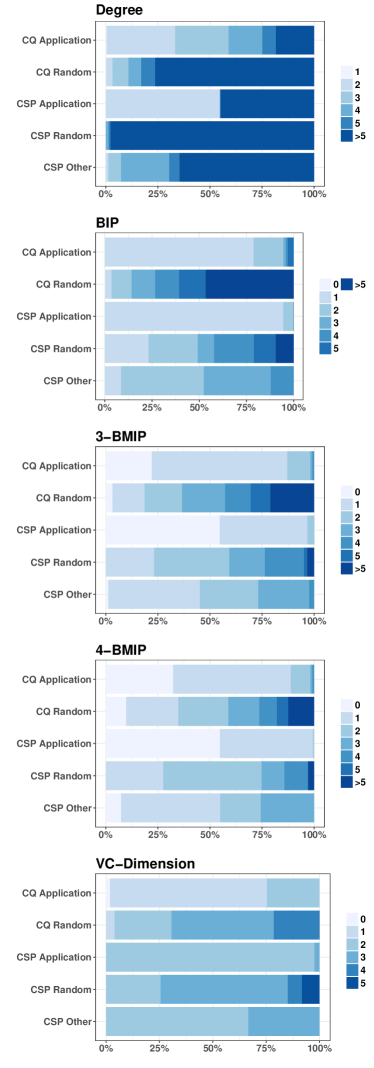
Figure 6. Hypergraph Properties

CQ Application
$k$	yes	no	timeout
$1$	454 (0)	81 (0)	0
$2$	73 (0)	8 (0)	0
$3$	8 (0)	0	0

CQ Random
$k$	yes	no	timeout
$1$	36 (0)	464 (0)	0
$2$	68 (0)	396 (0)	0
$3$	70 (0)	326 (32)	0
$4$	59 (0)	167 (544)	100
$5$	54 (0)	55 (610)	158
$10$	206 (5)	0	7
$15$	7 (0)	0	0

CSP Application
$k$	yes	no	timeout
$1$	0	1090 (0)	0
$2$	29 (0)	1061 (0)	0
$3$	116 (0)	802 (736)	143
$4$	283 (18)	62 (707)	600
$5$	231 (13)	0	431
$10$	261 (0)	0	170
$15$	12 (0)	0	158
$25$	118 (0)	0	40
$50$	40 (0)	0	0

CSP Random
$k$	yes	no	timeout
$1$	0	863 (0)	0
$2$	47 (0)	816 (1)	0
$3$	111 (0)	602 (1319)	103
$4$	39 (42)	160 (1332)	506
$5$	136 (59)	0	530
$10$	530 (0)	0	0

CSP Other
$k$	yes	no	timeout
$1$	0	82 (1)	0
$2$	19 (0)	55 (219)	8
$3$	5 (0)	11 (1257)	47
$4$	5 (0)	2 (943)	51
$5$	6 (0)	1 (0)	46
$10$	24 (0)	0	23
$15$	6 (1)	0	17
$25$	7 (10)	0	10
$50$	5 (0)	0	5
$75$	4 (0)	0	1

Table 9. HW of instances with average runtime in s

In Figure 2, the results of our $\mathit{hw}$-analysis were presented. In Table 9 and Figure 7, additional details are provided by distinguishing the three classes of CSP instances. As in Figure 2, we also write the average runtimes in the bars of Figure 7. In the tabular presentation in Table 9, this information is given by putting the number of seconds in parentheses.

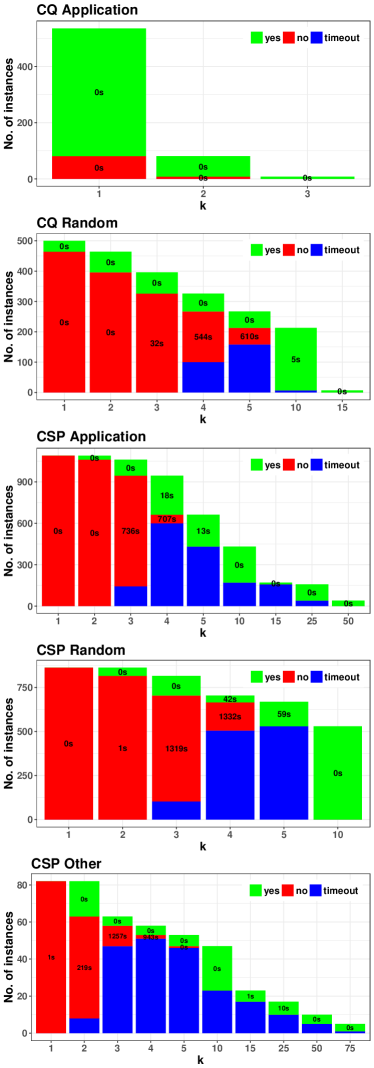
Figure 7. HW analysis (labels are average runtimes in s)

Appendix D Further Details for Section 5

In Table 4, we gave an overview of the improvements of the width when switching from $\mathit{hw}$ to $\mathit{ghw}$. In Table 10 and Figure 8, additional details are provided by distinguishing the three classes of CSP instances. The runtimes are given in parentheses in the tabular representation and in the bars of the bar chart, respectively. The pseudocode of the GHD-algorithm via balanced separators is given in Figure 9.

CQ Applicatoin
$\mathit{hw}\rightarrow\mathit{ghw}$	yes	no	timeout
$3\rightarrow 2$	0	8 (0)	0
CQ Random
$\mathit{hw}\rightarrow\mathit{ghw}$	yes	no	timeout
$3\rightarrow 2$	0	70 (29)	0
$4\rightarrow 3$	0	48 (65)	11
$5\rightarrow 4$	0	30 (41)	24
$6\rightarrow 5$	0	29 (655)	40
CSP Application
$\mathit{hw}\rightarrow\mathit{ghw}$	yes	no	timeout
$3\rightarrow 2$	0	116 (7)	0
$4\rightarrow 3$	0	173 (66)	110
$5\rightarrow 4$	0	32 (9)	199
$6\rightarrow 5$	8 (41)	29 (458)	74
CSP Random
$\mathit{hw}\rightarrow\mathit{ghw}$	yes	no	timeout
$3\rightarrow 2$	0	111 (0)	0
$4\rightarrow 3$	0	38 (0)	1
$5\rightarrow 4$	0	86 (4)	50
$6\rightarrow 5$	9 (221)	121 (47)	141
CSP Other
$\mathit{hw}\rightarrow\mathit{ghw}$	yes	no	timeout
$3\rightarrow 2$	0	4 (14)	1
$4\rightarrow 3$	0	3 (120)	2
$5\rightarrow 4$	0	0	6
$6\rightarrow 5$	1 (2)	1 (2)	6

Table 10. GHW of instances with average runtime in s

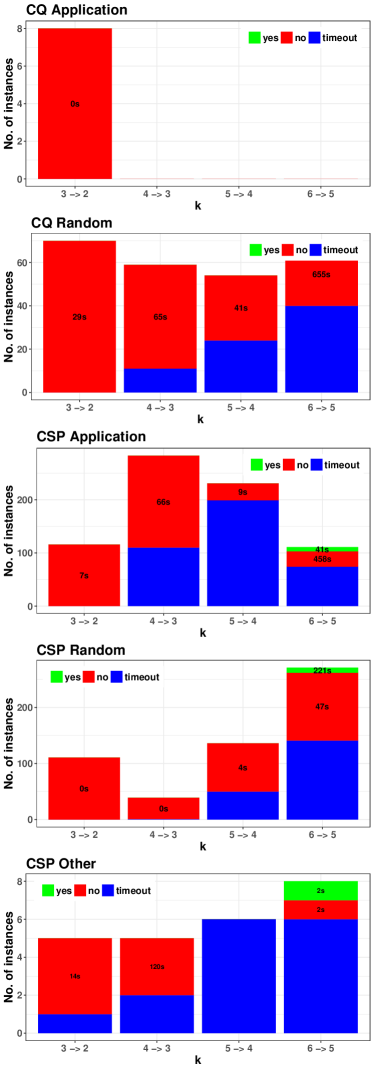
Figure 8. GHW analysis (labels are average runtime in s)

ALGORITHM Find_GHD_via_balancedSeparators // high-level sketch Input:    hypergraph $H^{\prime}$, integer $k\geq 0$. Output: a GHD $\left<T,B_{u},\lambda_{u}\right>$ of width $\leq k$ if exists,             “Reject”, otherwise. Procedure Find_GHD ($H$: Hypergraph, $\mathit{Sp}$: Set of Special-Edges) begin // 1. Stop if there are at most two special edges left: If $E(H)=\emptyset$ and $|\mathit{Sp}|\leq 2$ then return a GHD having a node for each $s\in\mathit{Sp}$ with $B_{u}:=s$ and $\lambda_{u}:=\{s\}$; // 2. Find a balanced separator $\lambda_{u}$ for $H$: Guess a balanced separator $\lambda_{u}\subseteq E(H^{\prime})$ with $|\lambda_{u}|\leq k$ for root $u$ of a GHD of $H$ such that: $\bullet\quad B(\lambda_{u})\not\in\mathit{Sp}$ $\bullet\quad B(\lambda_{u})\subseteq V(H)$ If no such balanced separator exists then return Reject; $B_{u}:=B(\lambda_{u})$; // 3. Split $H$ into connected components $C_{1},\dots,C_{\ell}$ w.r.t. $\lambda_{u}$: $V_{u}:=V(H)\setminus B_{u}$; $E_{u}:=\{e\cap V_{u}\mid e\in(E(H)\cup\mathit{Sp})\}$; Compute the connected components of $(V_{u},E_{u})$ Let the connected components be denoted by $C_{1},\dots,C_{\ell}$; // 4. Build the pairs $\left<H_{i},\mathit{Sp}_{i}\right>$ for each connected component $C_{i}$: For every $i\in\{1,\dots,\ell\}$ do $E_{i}:=\{e\mid e\in E(H)$ and $e\cap C_{i}\neq\emptyset\}$; $V_{i}:=V(E_{i})\cup B_{u}$; Let $H_{i}$ be the hypergraph $(V_{i},E_{i})$; $\mathit{Sp}_{i}:=\{s\in\mathit{Sp}\mid s\cap C_{i}\neq\emptyset\}\cup\{B_{u}\}$; od; // 5. Call Find_GHD($H_{i}$, $\mathit{Sp}_{i}$) for each pair $\left<H_{i},\mathit{Sp}_{i}\right>$: For each $i\in\{1,\dots,\ell\}$ $T_{i}:=$ Find_GHD ($H_{i}$, $\mathit{Sp}_{i}$) If $\exists i$ s.t. recursive call returns Reject then return Reject; // 6. Create and return a new GHD for $H$ having $B_{u}$ and $\lambda_{u}$ as root: Create a new root $u$ with $B_{u}$ and $\lambda_{u}$; Reroot all $T_{i}$ at the node $t_{i}$ where $\lambda_{t_{i}}=\{B_{u}\}$; Attach all children of $t_{i}$ to $u$; return the new GHD rooted at $u$; end begin (* Main *) return Find_GHD ($H^{\prime}$, $\emptyset$); end

Figure 9. Recursive GHD-algorithm via balanced separators

Appendix E Further Details for Section 6

In Table 5, we presented the achieved improvements of the width by switching from integral covers of HDs to fractional covers. In Tables 11 and  12 and Figures 10 and 11, additional details are provided by distinguishing the three classes of CSP instances and by showing the results of the two algorithms SimpleImproveHD (in Table 11 and Figure 10) and FracImproveHD (in Table 12 and Figure 11) separately.

CQ Application
$\mathit{hw}$	$\geq 1$	$\geq 0.5$	$\geq 0.1$	no	timeout
$2$	0	17	0	56	0
$3$	0	0	0	8	0
CQ Random
$\mathit{hw}$	$\geq 1$	$\geq 0.5$	$\geq 0.1$	no	timeout
2	0	24	7	37	0
3	6	18	10	36	0
4	8	19	2	30	0
5	14	8	5	27	0
6	12	15	9	35	0
CSP Application
$\mathit{hw}$	$\geq 1$	$\geq 0.5$	$\geq 0.1$	no	timeout
$2$	0	0	0	29	0
$3$	0	0	0	116	0
$4$	0	7	0	276	0
$5$	0	5	0	226	0
$6$	0	6	0	105	0
CSP Random
$\mathit{hw}$	$\geq 1$	$\geq 0.5$	$\geq 0.1$	no	timeout
$2$	0	0	18	29	0
$3$	6	86	15	4	0
$4$	1	29	9	0	0
$5$	6	1	6	123	0
$6$	0	39	70	162	0
CSP Other
$\mathit{hw}$	$\geq 1$	$\geq 0.5$	$\geq 0.1$	no	timeout
$2$	0	0	0	20	0
$3$	0	0	0	5	0
$4$	0	0	0	5	0
$5$	0	0	0	6	0
$6$	0	0	1	7	0

Table 11. SimpleImproveHD of instances

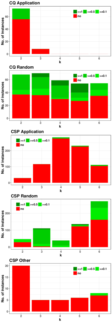
Figure 10. SimpleImproveHD analysis

CQ Application
$\mathit{hw}$	$\geq 1$	$\geq 0.5$	$\geq 0.1$	no	timeout
$2$	0	20	0	53	0
$3$	0	0	0	8	0
CQ Random
$\mathit{hw}$	$\geq 1$	$\geq 0.5$	$\geq 0.1$	no	timeout
$2$	0	26	7	35	0
$3$	7	29	5	6	23
$4$	10	23	1	6	19
$5$	12	19	4	1	18
$6$	14	26	7	0	22
CSP Application
$\mathit{hw}$	$\geq 1$	$\geq 0.5$	$\geq 0.1$	no	timeout
$2$	0	0	0	29	0
$3$	0	0	0	116	0
$4$	0	21	0	2	260
$5$	0	83	0	1	147
$6$	1	28	0	2	80
CSP Random
$\mathit{hw}$	$\geq 1$	$\geq 0.5$	$\geq 0.1$	no	timeout
$2$	0	0	22	25	0
$3$	7	87	16	1	0
$4$	1	37	1	0	0
$5$	6	24	55	0	51
$6$	12	94	87	3	75
CSP Other
$\mathit{hw}$	$\geq 1$	$\geq 0.5$	$\geq 0.1$	no	timeout
$2$	0	0	0	18	1
$3$	0	0	0	4	1
$4$	0	0	0	1	4
$5$	0	0	0	1	5
$6$	1	1	1	1	4

Table 12. FracImproveHD of instances

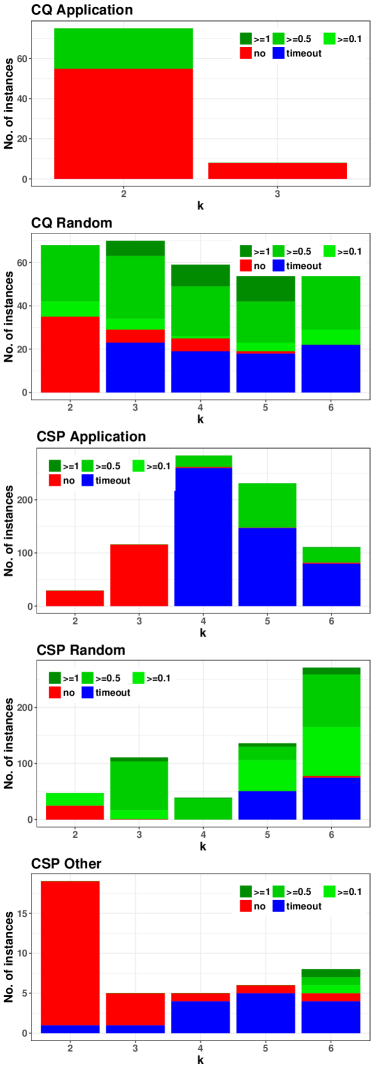
Figure 11. FracImproveHD analysis

References

- (1)
- Aberger et al. (2017) Christopher R. Aberger, Andrew Lamb, Susan Tu, Andres Nötzli, Kunle Olukotun, and Christopher Ré. 2017. EmptyHeaded: A Relational Engine for Graph Processing. ACM Trans. Database Syst. 42, 4 (2017), 20:1–20:44.
- Aberger et al. (2016a) Christopher R. Aberger, Susan Tu, Kunle Olukotun, and Christopher Ré. 2016a. EmptyHeaded: A Relational Engine for Graph Processing. In Proc. SIGMOD 2016. ACM, 431–446.
- Aberger et al. (2016b) Christopher R. Aberger, Susan Tu, Kunle Olukotun, and Christopher Ré. 2016b. Old Techniques for New Join Algorithms: A Case Study in RDF Processing. CoRR abs/1602.03557 (2016). http://arxiv.org/abs/1602.03557
- Adler et al. (2007) Isolde Adler, Georg Gottlob, and Martin Grohe. 2007. Hypertree width and related hypergraph invariants. Eur. J. Comb. 28, 8 (2007), 2167–2181.
- Amroun et al. (2016) Kamal Amroun, Zineb Habbas, and Wassila Aggoune-Mtalaa. 2016. A compressed Generalized Hypertree Decomposition-based solving technique for non-binary Constraint Satisfaction Problems. AI Commun. 29, 2 (2016), 371–392.
- Aref et al. (2015) Molham Aref, Balder ten Cate, Todd J. Green, Benny Kimelfeld, Dan Olteanu, Emir Pasalic, Todd L. Veldhuizen, and Geoffrey Washburn. 2015. Design and Implementation of the LogicBlox System. In Proc. SIGMOD 2015. ACM.
- Arocena et al. (2015) Patricia C. Arocena, Boris Glavic, Radu Ciucanu, and Renée J. Miller. 2015. The iBench Integration Metadata Generator. Proc. VLDB Endow. 9, 3 (Nov. 2015), 108–119.
- Atserias et al. (2013) Albert Atserias, Martin Grohe, and Dániel Marx. 2013. Size Bounds and Query Plans for Relational Joins. SIAM J. Comput. 42, 4 (2013), 1737–1767.
- Audemard et al. (2016) Gilles Audemard, Frédéric Boussemart, Christoph Lecoutre, and Cédric Piette. 2016. XCSP3: an XML-based format designed to represent combinatorial constrained problems. http://xcsp.org. (2016).
- Bakibayev et al. (2013) Nurzhan Bakibayev, Tomás Kociský, Dan Olteanu, and Jakub Závodný. 2013. Aggregation and Ordering in Factorised Databases. PVLDB 6, 14 (2013).
- Benedikt (2017) Michael Benedikt. 2017. CQ benchmarks. (2017). Personal Communication.
- Benedikt et al. (2017) Michael Benedikt, George Konstantinidis, Giansalvatore Mecca, Boris Motik, Paolo Papotti, Donatello Santoro, and Efthymia Tsamoura. 2017. Benchmarking the Chase. In Proc. PODS 2017. ACM, 37–52.
- Berg et al. (2017) Jeremias Berg, Neha Lodha, Matti Järvisalo, and Stefan Szeider. 2017. MaxSAT Benchmarks based on Determining Generalized Hypertree-width. MaxSAT Evaluation 2017 (2017), 22.
- Bonifati et al. (2017) Angela Bonifati, Wim Martens, and Thomas Timm. 2017. An Analytical Study of Large SPARQL Query Logs. PVLDB 11, 2 (2017), 149–161. http://www.vldb.org/pvldb/vol11/p149-bonifati.pdf
- Carmeli et al. (2017) Nofar Carmeli, Batya Kenig, and Benny Kimelfeld. 2017. Efficiently Enumerating Minimal Triangulations. In Proc. PODS 2017. ACM, 273–287.
- Chandra and Merlin (1977) Ashok K. Chandra and Philip M. Merlin. 1977. Optimal Implementation of Conjunctive Queries in Relational Data Bases. In Proc. STOC 1977. ACM, 77–90.
- Dechter (2003) Rina Dechter. 2003. Constraint Processing.
- Feige and Mahdian (2006) Uriel Feige and Mohammad Mahdian. 2006. Finding small balanced separators. In Proc. STOC 2006. ACM, 375–384. https://doi.org/10.1145/1132516.1132573
- Fichte et al. (2018) Johannes K. Fichte, Markus Hecher, Neha Lodha, and Stefan Szeider. 2018. An SMT Approach to Fractional Hypertree Width. In Proc. CP 2018 (LNCS), Vol. 11008. Springer, 109–127.
- Fischl et al. ([n. d.]) Wolfgang Fischl, Georg Gottlob, and Reinhard Pichler. [n. d.]. General and Fractional Hypertree Decompositions: Hard and Easy Cases. In Proc. PODS 2018.
- Fischl et al. (2017) Wolfgang Fischl, Georg Gottlob, and Reinhard Pichler. 2017. Tractable Cases for Recognizing Low Fractional Hypertree Width. viXra.org e-prints viXra:1708.0373 (2017). http://vixra.org/abs/1708.0373
- Geerts et al. (2014) Floris Geerts, Giansalvatore Mecca, Paolo Papotti, and Donatello Santoro. 2014. Mapping and cleaning. In Proc. ICDE 2014. IEEE, 232–243.
- Ghionna et al. (2007) Lucantonio Ghionna, Luigi Granata, Gianluigi Greco, and Francesco Scarcello. 2007. Hypertree Decompositions for Query Optimization. In Proc. ICDE 2007. IEEE Computer Society, 36–45. https://doi.org/10.1109/ICDE.2007.367849
- Ghionna et al. (2011) Lucantonio Ghionna, Gianluigi Greco, and Francesco Scarcello. 2011. H-DB: a hybrid quantitative-structural sql optimizer. In Proc. CIKM 2011. ACM, 2573–2576.
- Gottlob et al. (2016) Georg Gottlob, Gianluigi Greco, Nicola Leone, and Francesco Scarcello. 2016. Hypertree Decompositions: Questions and Answers. In Proc. PODS 2016. ACM, 57–74.
- Gottlob et al. (2002) Georg Gottlob, Nicola Leone, and Francesco Scarcello. 2002. Hypertree Decompositions and Tractable Queries. J. Comput. Syst. Sci. 64, 3 (2002), 579–627.
- Gottlob et al. (2009) Georg Gottlob, Zoltán Miklós, and Thomas Schwentick. 2009. Generalized Hypertree Decompositions: NP-hardness and Tractable Variants. J. ACM 56, 6 (2009), 30:1–30:32.
- Gottlob and Samer (2008) Georg Gottlob and Marko Samer. 2008. A backtracking-based algorithm for hypertree decomposition. ACM Journal of Experimental Algorithmics 13 (2008).
- Grohe and Marx (2014) Martin Grohe and Dániel Marx. 2014. Constraint Solving via Fractional Edge Covers. ACM Trans. Algorithms 11, 1 (2014), 4:1–4:20.
- Guo et al. (2005) Yuanbo Guo, Zhengxiang Pan, and Jeff Heflin. 2005. LUBM: A benchmark for OWL knowledge base systems. J. Web Sem. 3, 2-3 (2005), 158–182. https://doi.org/10.1016/j.websem.2005.06.005
- Habbas et al. (2015) Zineb Habbas, Kamal Amroun, and Daniel Singer. 2015. A Forward-Checking algorithm based on a Generalised Hypertree Decomposition for solving non-binary constraint satisfaction problems. J. Exp. Theor. Artif. Intell. 27, 5 (2015), 649–671. https://doi.org/10.1080/0952813X.2014.993507
- Jain et al. (2016) Shrainik Jain, Dominik Moritz, Daniel Halperin, Bill Howe, and Ed Lazowska. 2016. SQLShare: Results from a Multi-Year SQL-as-a-Service Experiment. In Proceedings of the 2016 International Conference on Management of Data (SIGMOD ’16). ACM, New York, NY, USA, 281–293. https://doi.org/10.1145/2882903.2882957
- Karakashian et al. (2011) Shant Karakashian, Robert J. Woodward, and Berthe Y. Choueiry. 2011. Reformulating R(*, m)C with Tree Decomposition. In SARA. AAAI.
- Khamis et al. (2015) Mahmoud Abo Khamis, Hung Q. Ngo, Christopher Ré, and Atri Rudra. 2015. Joins via Geometric Resolutions: Worst-case and Beyond. In Proc. PODS 2015.
- Khamis et al. (2016) Mahmoud Abo Khamis, Hung Q. Ngo, and Atri Rudra. 2016. FAQ: Questions Asked Frequently. In Proc. PODS 2016. 13–28.
- Lalou et al. (2009) Mohammed Lalou, Zineb Habbas, and Kamal Amroun. 2009. Solving Hypertree Structured CSP: Sequential and Parallel Approaches. In Proc. RCRA@AI*IA 2009.
- Leis et al. (2015) Viktor Leis, Andrey Gubichev, Atanas Mirchev, Peter Boncz, Alfons Kemper, and Thomas Neumann. 2015. How Good Are Query Optimizers, Really? PVLDB 9, 3 (Nov. 2015), 204–215. https://doi.org/10.14778/2850583.2850594
- Leis et al. (2017) Viktor Leis, Bernhard Radke, Andrey Gubichev, Atanas Mirchev, Peter Boncz, Alfons Kemper, and Thomas Neumann. 2017. Query optimization through the looking glass, and what we found running the Join Order Benchmark. The VLDB Journal (18 Sep 2017). https://doi.org/10.1007/s00778-017-0480-7
- Malyshev et al. (2018) Stanislav Malyshev, Markus Krötzsch, Larry González, Julius Gonsior, and Adrian Bielefeldt. 2018. Getting the Most out of Wikidata: Semantic Technology Usage in Wikipedia’s Knowledge Graph. In Proc. ISWC 2018. To appear.
- Marx (2010) Dániel Marx. 2010. Approximating Fractional Hypertree Width. ACM Trans. Algorithms 6, 2, Article 29 (2010), 29:1–29:17 pages.
- Moll et al. (2012) Lukas Moll, Siamak Tazari, and Marc Thurley. 2012. Computing hypergraph width measures exactly. Inf. Process. Lett. 112, 6 (2012), 238–242.
- Olteanu and Závodnỳ (2015) Dan Olteanu and Jakub Závodnỳ. 2015. Size bounds for factorised representations of query results. ACM Trans. Database Syst. 40, 1 (2015), 2.
- Perelman and Ré (2015) Adam Perelman and Christopher Ré. 2015. DunceCap: Compiling Worst-Case Optimal Query Plans. In Proc. SIGMOD 2015. ACM, 2075–2076.
- Picalausa and Vansummeren (2011) François Picalausa and Stijn Vansummeren. 2011. What are real SPARQL queries like?. In Proc. SWIM 2011. ACM, 7. https://doi.org/10.1145/1999299.1999306
- Pottinger and Halevy (2001) Rachel Pottinger and Alon Halevy. 2001. MiniCon: A Scalable Algorithm for Answering Queries Using Views. The VLDB Journal 10, 2-3 (Sept. 2001), 182–198.
- Scarcello et al. (2007) Francesco Scarcello, Gianluigi Greco, and Nicola Leone. 2007. Weighted hypertree decompositions and optimal query plans. J. Comput. Syst. Sci. 73, 3 (2007).
- Schafhauser (2006) Werner Schafhauser. 2006. New heuristic methods for tree decompositions and generalized hypertree decompositions. (2006). Master Thesis, TU Wien.
- Schild and Sommer (2015) Aaron Schild and Christian Sommer. 2015. On Balanced Separators in Road Networks. In Proc. SEA 2015 (LNCS), Vol. 9125. Springer, 286–297.
- Transaction Processing Performance Council (TPC) (2014) Transaction Processing Performance Council (TPC). 2014. TPC-H decision support benchmark. http://www.tpc.org/tpch/default.asp. (2014).
- Tu and Ré (2015) Susan Tu and Christopher Ré. 2015. Duncecap: Query plans using generalized hypertree decompositions. In Proc. SIGMOD 2015. ACM, 2077–2078.
- Vapnik and Chervonenkis (1971) Vladimir Vapnik and Alexey Chervonenkis. 1971. On the uniform convergence of relative frequencies of events to their probabilities. Theory Probab. Appl. 16 (1971), 264–280.