Hong-Ou-Mandel heat noise in the quantum Hall regime

Abstract

We investigate heat current fluctuations induced by a periodic train of Lorentzian-shaped pulses, carrying an integer number of electronic charges, in a Hong-Ou-Mandel interferometer implemented in a quantum Hall bar in the Laughlin sequence. We demonstrate that the noise in this collisional experiment cannot be reproduced in a setup with a single drive, in contrast to what is observed in the charge noise case. Nevertheless, the simultaneous collision of two identical levitons always leads to a total suppression even for the Hong-Ou-Mandel heat noise at all filling factors, despite the presence of emergent anyonic quasi-particle excitations in the fractional regime. Interestingly, the strong correlations characterizing the fractional phase are responsible for a remarkable oscillating pattern in the HOM heat noise, which is completely absent in the integer case. These oscillations can be related to the recently predicted crystallization of levitons in the fractional quantum Hall regime.

I Introduction

The recent progress in generating and controlling coherent few-particle excitations in quantum conductors opened the way to a new research field, known as electron quantum optics (EQO) Bocquillon et al. (2014); Grenier et al. (2011a). The main purpose of EQO is to reproduce conventional optics experiments using electronic wave-packets propagating in condensed matter systems instead of photons travelling along wave-guides.

In this context, a remarkable effort has been put forth by the condensed matter community to implement on-demand sources of electronic wave-packets in mesoscopic systems. After seminal theoretical works and groundbreaking experimental results, two main methods to realize single-electron sources assumed a prominent role in the field of EQO Dubois et al. (2013a); Grenier et al. (2013); Misiorny et al. (2018); Glattli and Roulleau (2017); Bäuerle et al. (2018). The first injection protocol relies on the periodic driving of the discrete energy spectrum of a quantum dot, which plays the role of a mesoscopic capacitor Büttiker (1993); Büttiker et al. (1993); Moskalets (2013). In this way, it is possible to achieve the periodic injection of an electron and a hole along the ballistic channels of a system coupled to this mesoscopic capacitor through a quantum point contact (QPC) Fève et al. (2007); Bocquillon et al. (2012); Parmentier et al. (2012); Ferraro et al. (2015).

A second major step has been the recent realization of an on-demand source of electron through the application of a time-dependent voltage to a quantum conductor Glattli and Roulleau (2017, 2016); Ferraro et al. (2018a); Misiorny et al. (2018); Moskalets (2016); Safi (2014); Dolcini (2017). The main challenge to face, in this case, has been that an ac voltage would generally excite unwanted neutral electron-hole pairs, thus spoiling at its heart the idea of a single-electron source. The turning point to overcome this issue was the theoretical prediction by Levitov and co-workers that a periodic train of quantized Lorentzian-shaped pulses, carrying an integer number of particles per period, is able to inject minimal single-electron excitations devoid of any additional electron-hole pair, then termed levitons Levitov et al. (1996); Ivanov et al. (1997); Keeling et al. (2006). Indeed, this kind of single-electron source is simple to realize and operate, since it relies on usual electronic components, and potentially provides a high level of miniaturization and scalability. For their fascinating properties Moskalets (2015), levitons have been proposed as flying qubits Glattli and Roulleau (2018) and as source of entanglement Dasenbrook and Flindt (2015); Dasenbrook et al. (2016); Dasenbrook and Flindt (2016); Ferraro et al. (2018b) with appealing applications for quantum information processing. Moreover, quantum tomography protocols able to reconstruct their single-electron wave-functions have been proposed Grenier et al. (2011b); Ferraro et al. (2013, 2014a) and experimentally realized Jullien et al. (2014).

While the implementation of single-electron sources has not been a trivial task, the condensed matter analogues of other quantum optics experimental components can be found in a more natural way. The wave-guides for photons can be replaced by the ballistic edge channels of mesoscopic devices, such as quantum Hall systems. Moreover, the role of electronic beam splitter, which should mimic the half-silvered mirror of conventional optics, can be played by a QPC, where electrons are reflected or transmitted with a tunable probability, which is typically assumed as energy independent. By combining these elements with the single-electron sources previously described, interferometric setups, originally conceived for optics experiments, can be implemented also in the condensed matter realm Ol’khovskaya et al. (2008); Rosselló et al. (2015). One famous example is the Hanbury-Brown-Twiss (HBT) interferometer Hanbury Brown and Twiss (1956a), where a stream of electronic wave-packets is excited along ballistic channels and partitioned against a QPC Bocquillon et al. (2012). The shot noise signal, generated due to the granular nature of electrons Martin (2005); Moskalets (2017), was employed to probe the single-electron nature of levitons in a non-interacting two-dimensional electron gas Glattli and Roulleau (2016); Dubois et al. (2013b). Its extension to the fractional quantum Hall regime was considered in Ref. Rech et al. (2017), where it was shown that levitons are minimal excitations also in strongly correlated edge channels.

A fundamental achievement of EQO has been the implementation of the Hong-Ou-Mandel (HOM) interferometer Hong et al. (1987), where electrons impinge on the opposite side of a QPC with a tunable delay Bocquillon et al. (2013); Glattli and Roulleau (2017); Dubois et al. (2013b). By performing this kind of collisional experiments, it is possible to gather information about the forms of the impinging electronic wave-packets and to measure their degree of indistinguishability Jonckheere et al. (2012); Ferraro et al. (2018a, 2015). For instance, when two indistinguishable and coherent electronic states collide simultaneously (zero time delay) at the QPC, charge current fluctuations are known to vanish at zero temperature, thus showing the so called Pauli dip Ferraro et al. (2014b); Glattli and Roulleau (2017); Dubois et al. (2013b). This dip can be interpreted in terms of anti-bunching effects related to the Fermi statistics of electrons. HOM experiments can thus be employed to test whether decoherence and dephasing, induced by electron-electron interactions, reduce the degree of indistinguishability of colliding electrons Wahl et al. (2014); Ferraro et al. (2014a); Freulon et al. (2015); Marguerite et al. (2016); Cabart et al. (2018).

As discussed above, the main driving force behind EQO has been to properly revise quantum optics experiments focusing on charge transport properties of single-electron excitations. Nevertheless, some recent groundbreaking experiments has spurred the investigation also in the direction of heat transport at the nanoscale Giazotto et al. (2006); Landauer (2015); Esposito et al. (2009); Campisi et al. (2011); Benenti et al. (2017); Li et al. (2012). In this context, the coherent transport and manipulation of heat fluxes have been reported in Josephson junctions Giazotto and Martínez-Pérez (2012); Martínez-Pérez et al. (2015); Fornieri et al. (2017) and quantum Hall systems Granger et al. (2009); Altimiras et al. (2010, 2012). Intriguingly, the quantization of heat conductance has been observed in integer Jezouin et al. (2013) and fractional quantum Hall systems Kane and Fisher (1997); Banerjee et al. (2017, 2018), which were already known for the extremely precise quantization of their charge conductance. In this way, ample and valuable information about these peculiar states of matter, which was not accessible by charge measurement, is now available with interesting implications also for quantum computation Simon (2018); Wang et al. (2018); Mross et al. (2018). New intriguing challenges posed by extending concepts like energy harvesting Sánchez et al. (2015a, b); Samuelsson et al. (2017); Thierschmann et al. (2015); Juergens et al. (2013); Erdman et al. (2017); Mazza et al. (2014), driven heat and energy transport Ronetti et al. (2017); Ludovico et al. (2014, 2016, 2018); Mazza et al. (2015), energy exchange in open systems Carrega et al. (2015, 2016) and fluctuation-dissipation theorems Campisi et al. (2009, 2015); Moskalets (2014); Averin and Pekola (2010) to the quantum realm resulted in a great progress of the field of quantum thermodynamics.

A new perspective on EQO has been also triggered by the rising interest for heat transport properties of single-electron excitations. Mixed-charge correlators Crépieux and Michelini (2014, 2016); Battista et al. (2014a) and heat fluctuations Battista et al. (2013, 2014b) produced by single-electron sources were investigated and, in particular, it was shown that levitons are minimal excitations also for heat transport Vannucci et al. (2017). In addition, heat current has revealed a useful resource for the full reconstruction of a single-electron wave-function Moskalets and Haack (2017).

Here, we address the problem of the heat noise generated by levitons injected in a HOM interferometer in the fractional quantum Hall regime. We consider a four terminal quantum Hall bar in the Laughlin sequence Laughlin (1983), where a single channel arises on each edge. Two terminals are contacted to time-dependent voltages, namely $V_{L}$ and $V_{R}$. Tunneling processes of quasi-particles are allowed by the presence of a QPC connecting the two edge states. In this case, charge noise generated in the HOM setup is identical to the one generated in a single-drive setup driven by the voltage $V_{L}-V_{R}$. Interestingly, we prove that this does not hold true anymore for heat noise, since it is possible to identify a contribution to HOM heat noise which is absent in a single-drive interferometer driven by $V_{L}-V_{R}$. In addition, we prove that the HOM heat noise always vanishes for a zero delay between the driving voltage, both for integer and fractional filling factors. Finally, we focus on the case of Lorentzian-shaped voltage carrying an integer number of electrons and we show that the HOM heat noise displays unexpected side dips in the fractional quantum Hall regime, which have no parallel in the integer regime. Intriguingly, the number of these side dips increases with the number of levitons injected per period. This result is consistent with the recently predicted phenomenon of charge crystallization of levitons in the fractional quantum Hall regime Ronetti et al. (2018).

The paper is organized as follows. In Sec. II, we introduce the model and the setup. Then, we evaluate charge and heat noises in Sec. III. In Sec. IV, we present our results focusing on the peculiar case of levitons. Finally, we draw the conclusions in Sec. V. Three Appendices are devoted to the technical aspects.

II Model

A quantum Hall bar in a four terminal geometry is depicted in Fig. 1. In the Laughlin sequence $\nu=\frac{1}{2n+1}$, with integer $n\geq 0$, a single chiral mode arises on each edge Laughlin (1983); Wen (1990). In the special case of integer quantum Hall effect at $\nu=1$ ($n=0$), the system is composed by ordinary fermions and the chiral edge states are one-dimensional Fermi liquids. This description fails for other filling factors, where the excitations are quasi-particles with fractional charge $-\nu e$ (with $e>0$). The low-energy properties of the Laughlin states are well captured by an hydrodynamical model formulated in terms of right-moving and left-moving bosonic edge modes $\Phi_{R/L}(x)$, which satisfy commutation relations $\left[\Phi_{R/L}(x),\Phi_{R/L}(y)\right]=\pm i\pi\mathrm{sign}\left(x-y\right)$. The free Hamiltonian of these edge modes is (we set $\hbar=1$ throughout the paper) Wen (1995)

$$H_{0}=\frac{v}{4\pi}\int dx\hskip 2.84526pt\sum\limits_{r=R,L}\left(\partial_{x}\Phi_{r}(x)\right)^{2}\leavevmode\nobreak\ ,$$ (1)

where $v$ is the velocity of propagation of right and left moving bosonic modes.
Terminals $1$ and $4$ are assumed to be connected to external time-dependent drives, while the remaining terminals are used to perform measurements. The charge densities, defined as

$$\rho_{R/L}(x)=\pm\frac{e\sqrt{\nu}}{2\pi}\partial_{x}\Phi_{R/L}(x),$$ (2)

are capacitively coupled to the gate potentials $\mathcal{V}_{R/L}(x,t)$ through the following gate Hamiltonian Dolcini et al. (2016); Dolcini and Rossi (2018)

$$H_{g}=\int dx\hskip 2.84526pt\left\{\mathcal{V}_{R}(x,t)\rho_{R}(x)+\mathcal{V}_{L}(x,t)\rho_{L}(x)\right\}.$$ (3)

The spatial dependence of the potentials is restricted to the region containing the semi-infinite contacts $1$ ($R$) and $4$ ($L$) by putting $\mathcal{V}_{R}(x,t)=\Theta(-(x+d))V_{R}(t)$ and $\mathcal{V}_{L}(x,t)=\Theta(x-d)V_{L}(t)$ (with $d>0$). Here, $V_{R/L}(t)=V_{R/L,dc}+V_{R/L,ac}(t)$ are periodic voltages, where $V_{R/L,dc}$ are time-independent dc components and $V_{R/L,ac}$ are pure periodic ac signals with period $\mathcal{T}=\frac{2\pi}{\omega}$, such that $\int_{0}^{\mathcal{T}}\frac{dt}{\mathcal{T}}V_{R/L}(t)=V_{R/L,dc}$. We remark that such modelization of the electromagnetic coupling between gate voltages and Hall bar occurs for gauge fixing with zero vector potential.

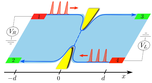
Figure 1: (Color online) Four-terminal setup for Hong-Ou-Mandel interferometry in the FQH regime. Contact 1 and 4 are used as input terminals, while contact 2 and 3 are the output terminals where current and noise are measured.

Since backscattering between the two edges is exponentially suppressed, we introduce a quantum point contact (QPC) at $x=0$, as shown in Fig. 1, in order to allow for tunneling events between right- and left-moving excitations. We assume the QPC is tuned to a very low transparency, i.e. in the weak backscattering regime, where the tunneling of fractional quasi-particles is the only relevant process Kane and Fisher (1992, 1994); Safi and Sukhorukov (2010). The corresponding additional term in the Hamiltonian is

$$H_{t}=\Lambda\leavevmode\nobreak\ \Psi^{\dagger}_{R}(0)\Psi_{L}(0)+\textit{H.c.}\leavevmode\nobreak\ ,$$ (4)

where we introduced the quasi-particle fields represented by the bosonization identity Giamarchi (2003); Martin (2005); Guyon et al. (2002)

$$\Psi_{R/L}(x)=\frac{\mathcal{F}_{R/L}}{\sqrt{2\pi a}}e^{-i\sqrt{\nu}\Phi_{R/L}(x)},$$ (5)

with $\mathcal{F}_{R/L}$ the so-called Klein factor, necessary for the proper anti-commutation relations, and $a$ the short-length cut-off.

III Noises in the double-drive configuration

The random partitioning, due to the poissonian tunneling at the QPC, generates fluctuations in the currents flowing along the quantum Hall bar. In this Section, we derive the expressions for charge and heat current noise in the double-drive configuration introduced in Sec. II, focusing on the regions downstream of the voltage contacts, namely $-d<x<d$.

III.1 Charge noise

We start by recalling the calculations for charge noise Dubois et al. (2013a); Rech et al. (2017); Glattli and Roulleau (2016). Charge current operators entering reservoirs $2$ and $3$ (located in $x=-d$ and $x=d$, respectively) can be expressed, due to chirality of Laughlin edge states, in terms of charge densities in Eq. (2)

$$j_{2/3}(t)=\pm v\rho_{R/L}(\pm d,t).$$ (6)

The zero frequency cross-correlated charge noise is

$$\mathcal{S}_{C}=\int_{0}^{\mathcal{T}}\frac{dt}{\mathcal{T}}\int_{-\infty}^{+\infty}dt^{\prime}\left[\left\langle j_{2}(t^{\prime})j_{3}(t)\right\rangle-\left\langle j_{2}(t^{\prime})\right\rangle\left\langle j_{3}(t)\right\rangle\right],$$ (7)

where the thermal average is performed over the initial equilibrium density matrix, in absence of tunneling and driving voltage. In the weak backscattering regime, standard perturbative approach in the tunneling Hamiltonian will be used. The total time evolution of charge current operators with respect to $H_{0}+H_{g}+H_{t}$ can be then constructed in terms of powers of $\Lambda$ and reads

$$j_{2/3}(t)=j^{(0)}_{2/3}(t)+j^{(1)}_{2/3}(t)+j^{(2)}_{2/3}(t)+\mathcal{O}(\left|\Lambda\right|^{3}),$$ (8)

with

$$j^{(0)}_{2/3}(t)=\pm v\rho_{R/L}^{(0)}(\pm d,t),$$ (9)

$$j^{(1)}_{2/3}(t)=\pm iv\int\limits_{-\infty}^{t}dt^{\prime}\left[H_{t}(t^{\prime}),\rho_{R/L}^{(0)}(\pm d,t)\right],$$ (10)

$$j^{(2)}_{2/3}(t)=\pm(i)^{2}v\int\limits_{-\infty}^{t}dt^{\prime}\int\limits_{-\infty}^{t^{\prime}}dt^{\prime\prime}\left[H_{t}(t^{\prime\prime}),\left[H_{t}(t^{\prime}),\rho_{R/L}^{(0)}(\pm d,t)\right]\right],$$ (11)

where the tunneling Hamiltonian $H_{t}(t)$ and the charge densities $\rho_{R/L}^{(0)}(x,t)$ evolve in the interaction picture with respect to $H_{0}+H_{g}$. In order to make explicit the form of $\rho_{R/L}^{(0)}(x,t)$ it is sufficient to solve the equations of motion for the bosonic fields $\Phi_{R/L}$ with respect to $H_{0}+H_{g}$, i.e. in the absence of tunneling. The solutions read

$$\Phi_{R/L}(x,t)=\phi_{R/L}(x,t)-e\sqrt{\nu}\int_{0}^{t\mp\frac{x}{v}-\frac{d}{v}}dsV_{R/L}(s),$$ (12)

where $\phi_{R/L}(x,t)=\phi_{R/L}(x\mp vt)$ are the chiral bosonic fields at equilibrium (zero applied drive).
By exploiting the commutator

$$\left[H_{t}(t^{\prime}),\rho^{(0)}_{R/L}(x,t)\right]=-\delta\left(t^{\prime}-\left(t\mp\frac{x}{v}\right)\right)\dot{N}_{R/L}(x,t),$$ (13)

where

$$\dot{N}_{R}\left(x,t\right) =i\nu e\Lambda\Psi_{R}^{\dagger}(x-vt,0)\Psi_{L}(x-vt,0)+\text{H.c.},$$ (14)

$$\dot{N}_{L}\left(x,t\right) =-i\nu e\Lambda\Psi_{R}^{\dagger}(x+vt,0)\Psi_{L}(x+vt,0)+\text{H.c.},$$ (15)

Eqs. (10) and (11) can be further recast as

$$j^{(1)}_{2/3}(t)=\dot{N}_{R/L}\left(\pm d,t\right),$$ (16)

$$j^{(2)}_{2/3}(t)=i\int\limits_{-\infty}^{t-\frac{d}{v}}dt^{\prime\prime}\left[H_{t}(t^{\prime\prime}),\dot{N}_{R/L}\left(\pm d,t\right)\right].$$ (17)

In these expressions, we introduced the time evolution of quasi-particle fields with respect to $H_{0}+H_{g}$, which can be obtained from Eq. (12) using the bosonization identity

$$\Psi_{R,L}(x,t)=\frac{\mathcal{F}_{R/L}}{\sqrt{2\pi a}}e^{-i\sqrt{\nu}\phi_{R/L}(x,t)}e^{i\nu e\int_{0}^{t\mp\frac{x}{v}-\frac{d}{v}}dt^{\prime}V_{R/L}(t^{\prime})},$$ (18)

The current noise can be obtained from Eqs. (9), (10): the only non-vanishing contribution to second order in $\Lambda$ comes from $j^{(1)}_{2}(t+\tau)j^{(1)}_{3}(t)$, with terms $j^{(0)}_{2}(t+\tau)j^{(2)}_{3}(t)$ and $j^{(2)}_{2}(t+\tau)j^{(0)}_{3}(t)$ averaging to zero.
By introducing the correlator ($k_{B}=1$)

$$P_{g}(t^{\prime}-t) =\langle e^{i\sqrt{g}\phi_{R/L}(0,t^{\prime})}e^{-i\sqrt{g}\phi_{R/L}(0,t)}\rangle=$$

$$=\left[\frac{\pi\theta\left(t^{\prime}-t\right)}{\sinh\left(\pi\theta\left(t^{\prime}-t\right)\right)\left(1+i\omega_{c}\left(t^{\prime}-t\right)\right)}\right]^{g},$$ (19)

with $\theta$ the temperature and $\omega_{c}=v/a$ the high energy cut-off, one finds ($\lambda=\frac{\Lambda}{2\pi a}$)

$$\mathcal{S}_{C}=-2(\nu e)^{2}|\lambda|^{2}\int_{0}^{\mathcal{T}}\frac{dt}{\mathcal{T}}\int_{-\infty}^{+\infty}dt^{\prime}\times$$

$$\times\cos\left\{\nu e\int_{t}^{t^{\prime}}V_{-}(\tau)d\tau\right\}P_{2\nu}(t^{\prime}-t),$$ (20)

where $V_{-}=V_{R}-V_{L}$.
Even though this charge noise is generated in a double-drive configuration, it is interesting to point out that it actually depends only on the single effective drive $V_{-}(t)$. The configuration with a single drive is usually termed in literature Hanbury-Brown-Twiss (HBT) setup Hanbury Brown and Twiss (1956a, b); Bocquillon et al. (2012); Dubois et al. (2013b).
Therefore, the charge noise presented in Eq. (20) is the same as the one generated in a single-drive configuration, where reservoir 4 is grounded ($V_{L}(t)=0$) and reservoir 1 is contacted to the periodic voltage $V_{-}(t)$, such that

$$S_{C}\left(V_{R},V_{L}\right)=S_{C}\left(V_{-},0\right).$$ (21)

Here, the arguments in brackets indicate the voltage applied to reservoirs $1$ and $4$, respectively.
One might consider Eq. (21) as a consequence of a trivial shift of both voltages by a value corresponding to $V_{L}$. Nevertheless, such a result cannot be obtained by means of a gauge transformation (see Appendix A). In this sense, Eq. (21) implies that the charge noise incidentally acquires the same expression in these two physically distinct experimental setups. As will be clearer in the following, for the charge case this is a consequence of the presence of a single local (energy independent) QPC. Generally, we expect that the double-drive and the single-drive ($V_{R}(t)=V_{-}(t)$ and $V_{L}(t)=0$) configurations return different outcomes for other physical observables, such as heat noise, as discussed in the next part.

III.2 Heat noise

In the following, we evaluate the correlation noise of heat current between terminal $2$ and $3$ in the double-drive configuration. The heat current operators of terminal $2$ and $3$ can be expressed in terms of heat density operators Kane and Fisher (1996)

$$\mathcal{Q}_{R/L}(x,t)=\frac{v}{4\pi}\left(\partial_{x}\Phi_{R/L}(x,t)\right)^{2},$$ (22)

as

$$\mathcal{J}_{2/3}(t)=\pm v\leavevmode\nobreak\ \mathcal{Q}_{R/L}(\pm d,t),$$ (23)

due to the chirality of Laughlin edge states.
Then, we can define the cross-correlated heat noise

$$\mathcal{S}_{Q}=\int_{0}^{\mathcal{T}}\frac{dt}{\mathcal{T}}\int dt^{\prime}\hskip 2.84526pt\left\{\langle\mathcal{J}_{2}(t^{\prime})\mathcal{J}_{3}(t)\rangle-\langle\mathcal{J}_{2}(t^{\prime})\rangle\leavevmode\nobreak\ \langle\mathcal{J}_{3}(t)\rangle\right\}\leavevmode\nobreak\ ,$$ (24)

Analogously to charge current, one can expand heat current operators in power of the tunneling amplitude $\Lambda$, thus obtaining

$$\mathcal{J}_{2/3}(t)=\mathcal{J}^{(0)}_{2/3}(t)+\mathcal{J}^{(1)}_{2/3}(t)+\mathcal{J}^{(2)}_{2/3}(t)+\mathcal{O}\left(\left|\Lambda\right|^{3}\right),$$ (25)

where

$$\mathcal{J}^{(0)}_{2/3}(t)=\pm v\mathcal{Q}^{(0)}_{R/L}(\pm d,t),$$ (26)

$$\mathcal{J}^{(1)}_{2/3}(t)=\pm iv\int\limits_{-\infty}^{t}dt^{\prime}\left[H_{t}(t^{\prime}),\mathcal{Q}^{(0)}_{R/L}(\pm d,t)\right],$$ (27)

$$\mathcal{J}^{(2)}_{2/3}(t)=\pm i^{2}v\int\limits_{-\infty}^{t}dt^{\prime}\int\limits_{-\infty}^{t^{\prime}}dt^{\prime\prime}\left[H_{t}(t^{\prime\prime}),\left[H_{t}(t^{\prime}),\mathcal{Q}^{(0)}_{R/L}(\pm d,t)\right]\right].$$ (28)

In the above equations we have denoted with $\mathcal{Q}^{(0)}(x,t)$, the time evolution of heat density in the absence of tunneling, which can be obtained from the time evolution of bosonic fields in Eq. (12) and reads

$$\mathcal{Q}^{(0)}_{R/L}(x,t)=\frac{v}{4\pi}\Big{[}\left(\partial_{x}\phi_{R/L}(x,t)\right)^{2}+$$

$$\pm e\sqrt{\nu}\partial_{x}\phi_{R/L}(x,t)V_{R/L}\left(t\mp\frac{x}{v}\right)+\frac{e^{2}\nu}{v}V^{2}_{R/L}\left(t\mp\frac{x}{v}\right)\Big{]}\leavevmode\nobreak\ .$$ (29)

The following commutator

$$\left[H_{t}(t^{\prime}),\mathcal{Q}^{(0)}_{R/L}(x,t)\right]=-i\delta\left(t^{\prime}-\left(t\mp\frac{x}{v}\right)\right)\dot{Q}_{R/L}(x,t),$$ (30)

where

$$\dot{Q}_{R}\left(x,t\right) =v\Lambda\left(\partial_{x}\Psi^{\dagger}_{R}(x,t)\right)\Psi_{L}(x,t)+\text{H.c.},$$ (31)

$$\dot{Q}_{L}\left(x,t\right) =-v\Lambda\Psi^{\dagger}_{R}(x,t)\left(\partial_{x}\Psi_{L}(x,t)\right)+\text{H.c.},$$ (32)

can be used to recast Eqs. (27) and (28)

$$\mathcal{J}^{(1)}_{2/3}(t)=\pm\dot{Q}_{R/L}\left(\pm d,t\right),$$ (33)

$$\mathcal{J}^{(2)}_{2/3}(t)=\pm i\int\limits_{-\infty}^{t-\frac{d}{v}}dt^{\prime\prime}\left[H_{t}(t^{\prime\prime}),\dot{Q}_{R/L}\left(\pm d,t\right)\right].$$ (34)

The perturbative expansion of heat current operator in Eq. (25) allows to express heat correlation noise to lowest order as

$$\mathcal{S}_{Q}=\mathcal{S}^{(02)}_{Q}+\mathcal{S}^{(20)}_{Q}+\mathcal{S}^{(11)}_{Q}+\mathcal{O}\left(\left|\Lambda\right|^{3}\right),$$ (35)

where

$$\mathcal{S}_{Q}^{(ij)}=\int_{0}^{\mathcal{T}}\frac{dt}{\mathcal{T}}\int dt^{\prime}\left\{\langle\mathcal{J}_{2}^{(i)}(t^{\prime})\mathcal{J}_{3}^{(j)}(t)\rangle-\langle\mathcal{J}_{2}^{(i)}(t^{\prime})\rangle\langle\mathcal{J}_{3}^{(j)}(t)\rangle\right\}.$$ (36)

Now, we can perform standard calculations, whose details are given in Appendix B, in order to evaluate all the terms appearing in Eq. (35). By using the result of this calculation, it is possible to check whether an expression analogous to Eq. (21) holds true also for heat noise. Interestingly, one finds that

$$\mathcal{S}_{Q}(V_{R},V_{L})=\mathcal{S}_{Q}(V_{-},0)+\Delta\mathcal{S}_{Q}(V_{R},V_{L}),$$ (37)

thus showing that, in contrast with the charge sector, heat fluctuations generated in the double-drive or in the single-drive configurations are different. The two contributions in Eq. (37) are

$$\mathcal{S}_{Q}(V_{-},0) =|\lambda|^{2}\int_{0}^{\mathcal{T}}\frac{dt}{\mathcal{T}}\int dt^{\prime}\Big{\{}\cos\left(\nu e\int_{t}^{t^{\prime}}d\tau V_{-}(\tau)\right)\Re\left[\mathcal{P}_{\nu}(t^{\prime}-t)\partial_{t}^{2}\mathcal{P}_{\nu}(t^{\prime}-t)\right]+$$

$$+\frac{\nu ev}{\pi}\int dt^{\prime\prime}V_{-}(t^{\prime})\mathcal{K}\left(t^{\prime},t,t^{\prime\prime}\right)\sin\left(\nu e\int_{t}^{t^{\prime}}d\tau V_{-}(\tau)\right)\Im\left[\partial_{t^{\prime\prime}}\mathcal{P}_{2\nu}(t^{\prime\prime}-t)\right]\Big{\}},$$ (38)

$$\Delta\mathcal{S}_{Q}(V_{R},V_{L}) =\nu^{2}e^{2}|\lambda|^{2}\int_{0}^{\mathcal{T}}\frac{dt}{\mathcal{T}}\int dt^{\prime}\cos\left(\nu e\int_{t}^{t^{\prime}}d\tau V_{-}(\tau)\right)\Big{(}\alpha_{RL}(t,t^{\prime})\Re\left[\mathcal{P}_{2\nu}(t^{\prime}-t)\right]+\beta_{RL}(t,t^{\prime})\Im\left[\mathcal{P}_{2\nu}(t^{\prime}-t)\right]\Big{)},$$ (39)

where we defined the following functions

$$\mathcal{K}(t^{\prime},t,t^{\prime\prime})=\int d\tau\mathcal{P}_{2}(t^{\prime}-\tau)\left(\Theta(\tau-t^{\prime\prime})-\Theta(\tau-t)\right)=$$

$$=\frac{\pi\theta}{v}\frac{\sinh\left(\pi\theta(t-t^{\prime\prime})\right)}{\sinh\left(\pi\theta(t^{\prime}-t)\right)\sinh\left(\pi\theta(t^{\prime}-t^{\prime\prime})\right)},$$ (40)

$$\alpha_{RL}(t,t^{\prime})=\left(V_{R}(t)V_{L}(t^{\prime})-V_{L}(t)V_{R}(t^{\prime})\right),$$ (41)

$$\beta_{RL}=\frac{v}{\pi}\int dt^{\prime\prime}\mathcal{K}(t^{\prime\prime},t,t^{\prime})V_{R}(t^{\prime\prime})\left[V_{L}(t^{\prime})-V_{L}(t)\right].$$ (42)

The result of Eq. (37) arises because heat noise is sensitive to the energy distribution of the injected particles, thus leading to different outcomes in the single- and double-drive configurations. In this light, we expect this to hold true for general energy-dependent phenomena occurring at the QPC. For instance, any similarity between charge noises generated in the two setups discussed previously would disappear for more complicated tunneling geometry, such as multiple QPC or extended contacts, where transmission functions become energy-dependent Chevallier et al. (2010); Dolcetto et al. (2012); Vannucci et al. (2015); Ronetti et al. (2016).
Eq. (37) further indicates that the double-drive and the single-drive configurations are completely distinct setups and that the relation in Eq. (21) is solely a contingent effect of the single local QPC geometry.
It is useful to express heat correlation noise in energy space, by introducing the following Fourier series

$$\nu eV_{R/L}(t) =\sum_{k}c_{k,R/L}e^{ik\omega t},$$ (43)

$$e^{-i\nu e\int_{0}^{t}d\tau V_{-}(\tau)} =\sum_{l}\tilde{p}_{l}e^{-i(l+q_{R}-q_{L})\omega t},$$ (44)

where we defined also the number of particles excited by $V_{R/L}$ along the system in a period

$$q_{R/L}=\frac{\nu e}{2\pi}\int_{0}^{\mathcal{T}}dt\hskip 2.84526ptV_{R/L}(t)=\frac{\nu eV_{R/L,dc}}{\omega},$$ (45)

and the Fourier transform of $P_{g}(t)$ in Eq. (19)

$$\tilde{\mathcal{P}}_{g}(E) =\int dt\mathcal{P}_{g}(t)e^{iEt}=$$

$$=\left(\frac{2\pi\theta}{\omega_{c}}\right)^{g-1}\frac{e^{\frac{E}{2\theta}}}{\Gamma(g)\omega_{c}}\left|\Gamma\left(\frac{g}{2}-i\frac{E}{2\pi\theta}\right)\right|^{2}.$$ (46)

By exploiting these results, the two contributions to $\mathcal{S}_{Q}$ become

$$\mathcal{S}_{Q}(V_{-},0)=-\left|\lambda\right|^{2}\sum_{l}\Big{\{}\frac{2\nu^{2}\pi^{2}\theta^{2}+(1+\nu)\left((l+q_{R}-q_{L})\omega\right)^{2}}{1+2\nu}\left|\tilde{p}_{l}\right|^{2}\tilde{\mathcal{P}}_{2\nu}((l+q_{R}-q_{L})\omega)+$$

$$-\frac{1}{4}\sum_{k\neq 0}\left(c_{k,R}-c_{k,L}\right)\left(\tilde{p}_{l-k}\tilde{p}^{*}_{l}-\tilde{p}_{l}\tilde{p}^{*}_{l+k}\right)(l+q_{R}-q_{L})\omega\coth\frac{k\omega}{2\theta}\left(\tilde{\mathcal{P}}_{2\nu}((l+q_{R}-q_{L})\omega)-\tilde{\mathcal{P}}_{2\nu}(-(l+q_{R}-q_{L})\omega)\right)\Big{\}},$$ (47)

$$\Delta\mathcal{S}_{Q}(V_{R},V_{L})=\frac{\left|\lambda\right|^{2}}{2}\sum_{k,p,l}\left(c_{k,R}c_{p,L}-c_{k,L}c_{p,R}\right)\tilde{p}_{l+k+p}\tilde{p}^{*}_{l}\frac{\mathcal{W}_{(l+q_{R}-q_{L}),k,p}+\mathcal{W}_{(l+q_{R}-q_{L}),p,k}}{2},$$ (48)

where the coefficients $\mathcal{W}_{l,k,p}$ encodes all the effects due to temperature and interaction on $\Delta\mathcal{S}_{Q}$ and reads

$$\mathcal{W}_{l,k,p}=\frac{\omega_{c}}{4\pi}\int\frac{dE}{2\pi}\Big{\{}\tilde{\mathcal{P}}_{1}(E) \tilde{\mathcal{P}}_{1}(k\omega-E)\Big{[}\tilde{\mathcal{P}}_{2\nu-1}(E-l\omega)+\tilde{\mathcal{P}}_{2\nu-1}(-E-(l+k+p)\omega)+\tilde{\mathcal{P}}_{2\nu-1}(-E+l\omega)\Big{]}+$$

$$+\tilde{\mathcal{P}}_{2\nu-1}(E+(l+k+p)\omega)\Big{\}}-\frac{1}{2}\left(\tilde{\mathcal{P}}_{2\nu}((l+k)\omega)+\tilde{\mathcal{P}}_{2\nu}(-(l+k)\right).$$ (49)

Let us observe that the contribution $\Delta\mathcal{S}_{Q}$ exists only in the double-drive configurations. Indeed, in the configuration with a single drive, where $V_{L}=0$, one obtains that $c_{k,L}=0$ for each $k$, and the contribution in Eq. (48) vanishes.

III.3 Hong-Ou-Mandel noises

Among all the possible choices for the configuration involving the two voltages $V_{R}$ and $V_{L}$, one of the most interesting, even from the experimental point of view, is the Hong-Ou-Mandel (HOM) setup, where two identical voltage drives are applied to reservoirs $1$ and $4$ and delayed by a constant time $t_{D}$. This experimental configuration corresponds to set $V_{R}(t)=V(t)$ and $V_{L}(t)=V(t+t_{D})$ in Eq. (20), with $V(t)$ a generic periodic drive. In this situation the charge excited by each drive along the edge channels are equal, such that $q_{R}=q_{L}=q$.
For notational convenience, we define the single-drive heat noise and the HOM charge and heat noises as

$$\mathcal{S}^{sd}_{Q} =\mathcal{S}_{Q}(V_{-}(t),0),$$ (50)

$$\mathcal{S}^{HOM}_{C/Q} =\mathcal{S}_{C/Q}(V(t),V(t+t_{D})).$$ (51)

According to Eq. (37) and using the above definitions, the HOM heat noise can be expressed as

$$\mathcal{S}_{Q}^{HOM}=\mathcal{S}_{Q}^{sd}+\Delta\mathcal{S}_{Q}.$$ (52)

From the existing literature Dubois et al. (2013a); Rech et al. (2017); Ronetti et al. (2018), it is well established that charge HOM noise reduces to its equilibrium value for null time delay. Before entering into the details of our discussion, we would like to prove analytically that the same holds true for HOM heat noise $\mathcal{S}_{Q}^{HOM}$, independently of the choice of any parameter. The photo-assisted amplitude in Eq. (44) reduces to $\tilde{p}_{l}=\delta_{l,0}$ and the Fourier coefficients $c_{k,-}$ vanish for all $k$. Let us start by looking at the single-drive contribution. By substituting this analytical simplification in Eq. (47), we obtain

$$\mathcal{S}_{Q}^{sd}(t_{D}=0)=-\left|\lambda\right|^{2}\frac{\nu^{2}\pi^{2}\theta^{2}}{1+2\nu}\equiv\mathcal{S}_{Q}^{vac},$$ (53)

which is independent of the injected particles and correspond simply to the equilibrium noise $\mathcal{S}_{Q}^{vac}$ due to thermal fluctuations. This can be clearly understood given the fact that $V_{-}(t)=0$ for $t_{D}=0$ and the single-drive contribution corresponds to the noise generated in a driveless configuration.
Concerning the remaining part in Eq. (52), one has for $t_{D}=0$

$$\Delta\mathcal{S}_{Q}=\frac{\left|\lambda\right|^{2}}{4}\sum_{k}c_{k,R}c_{-k,R}\left(\mathcal{W}_{0,k,-k}+\mathcal{W}_{0,-k,k}\right),$$ (54)

where

$$\mathcal{W}_{0,k,-k}=\frac{\tilde{\mathcal{P}}_{2\nu}(k\omega)-\tilde{\mathcal{P}}_{2\nu}(-k\omega)}{2}.$$ (55)

From Eq. (55), we can clearly deduce that $\mathcal{W}_{0,k,-k}=-\mathcal{W}_{0,-k,k}$, which enforces the vanishing of $\Delta\mathcal{S}_{Q}$ in Eq. (54). This is enough to prove that HOM heat noise always reaches its equilibrium value at $t_{D}=0$, such that

$$\mathcal{S}_{Q}^{HOM}(t_{D}=0)=\mathcal{S}_{Q}^{sd}(t_{D}=0)=\mathcal{S}_{Q}^{vac}.$$ (56)

Let us note that this is not a trivial result since $\mathcal{S}_{Q}^{HOM}$ does not depend effectively on the single drive $V_{-}$ as $\mathcal{S}_{Q}^{sd}$, but on both $V_{R}$ and $V_{L}$ and even at $t_{D}=0$ the system is still driven by these two voltages.

IV Results and discussions

In this section, we discuss the results concerning the heat correlation noises in the HOM interferometer. In particular, we focus our discussion on a specific driving voltage, namely a periodic train of Lorentzian pulses

$$V_{Lor}(t)=\frac{V_{0}}{\pi}\sum\limits_{k=-\infty}^{+\infty}\frac{W}{W^{2}+(t-k\mathcal{T})^{2}}.$$ (57)

A Lorentzian-shaped drive, which satisfy the additional quantization condition

$$\nu e\int_{0}^{\mathcal{T}}dt\hskip 2.84526ptV_{Lor}(t)=2\pi q,$$ (58)

with $q$ an integer number, constitutes the optimal driving able to inject clean pulses devoid of any additional electron-hole pairs. The minimal excitations thus emitted into the quantum Hall channels are the aforementioned levitons Levitov et al. (1996); Keeling et al. (2006). The Fourier coefficients for this specific drive are given in Appendix C.
In the HOM setup previously described, a state composed by $q_{L}=q_{R}=q$ levitons Moskalets (2018) is injected by each driven contact and collide at the QPC, separated by a controllable time delay.
In analogy with the previous literature on charge noise, we introduce the following ratio Wahl et al. (2014); Ferraro et al. (2013); Rech et al. (2017); Marguerite et al. (2016)

$$\mathcal{R}_{C/Q}^{HOM}=\frac{\mathcal{S}^{HOM}_{C/Q}-\mathcal{S}_{C/Q}^{vac}}{2\mathcal{S}^{R}_{C/Q}-2\mathcal{S}_{C/Q}^{vac}},$$ (59)

where we subtracted the equilibrium noise $\mathcal{S}_{C/Q}^{vac}$ and we normalize with respect to $\mathcal{S}_{C/Q}^{R}\equiv\mathcal{S}_{C/Q}(V_{R},0)$, which are charge and heat noises expected for the random partitioning of a single source of levitons, i.e. when $V_{R}(t)=V_{Lor}(t)$ and $V_{L}(t)=0$. The expressions for $\mathcal{S}_{C}^{vac}$ and $\mathcal{S}_{C}^{R}$ are well-known and have been derived in previous paper Rech et al. (2017); Vannucci et al. (2017); Dubois et al. (2013a). The expression for $\mathcal{S}_{Q}^{R}$ can be obtained from our results in Sec. III.2 and reads

$$\mathcal{S}_{Q}^{R}=-\left|\lambda\right|^{2}\sum_{l}\Big{\{}\frac{2\nu^{2}\pi^{2}\theta^{2}+(1+\nu)\left(l\omega\right)^{2}}{1+2\nu}\left|p_{l}\right|^{2}\tilde{\mathcal{P}}_{2\nu}((l+q)\omega)+$$

$$-\sum_{k\neq 0}c_{k}\left(p_{l-k}p^{*}_{l}-p_{l}p^{*}_{l+k}\right)(l+q)\omega\frac{\tilde{\mathcal{P}}_{2}(k\omega)}{2k\omega}\times$$

$$\times\left(\tilde{\mathcal{P}}_{2\nu}((l+q)\omega)-\tilde{\mathcal{P}}_{2\nu}(-(l+q)\omega)\right)\Big{\}},$$ (60)

where $c_{k}=\nu e\int_{0}^{\mathcal{T}}\frac{dt}{\mathcal{T}}V_{Lor}(t)e^{ik\omega t}$ are the Fourier coefficients for a single Lorentzian voltage and $p_{l}=\int_{0}^{\mathcal{T}}\frac{dt}{\mathcal{T}}e^{-i\nu e\int_{0}^{t}d\tau V_{lor}(\tau)}e^{i(l+q)\omega t}$ (see Appendix C).
In addition, we define an analogous ratio for single-drive heat noise as

$$\mathcal{R}_{Q}^{sd}=\frac{\mathcal{S}^{sd}_{Q}-\mathcal{S}_{Q}^{vac}}{2\mathcal{S}^{R}_{Q}-2\mathcal{S}_{Q}^{vac}},$$ (61)

in order to asses its relative contribution to the overall HOM heat noise.
Let us notice that, according to Eqs (53) and (56) both ratios, $\mathcal{R}_{Q}^{HOM}$ and $\mathcal{R}_{Q}^{sd}$ vanish for $t_{D}=0$. In the specific case of levitons, which are single-electron excitations, at $\nu=1$ the physical explanation for the total dip at $t_{D}=0$ involves the anti-bunching effect of identical fermions: electron-like excitations colliding at the QPC at the same time are forced to escape on opposite channels, thus leading to a total suppression of fluctuations at $t_{D}=0$ and generating the so called Pauli dip Dubois et al. (2013b); Jonckheere et al. (2012); Bocquillon et al. (2012). For fractional filling factors, it is remarkable that this total dip is still present despite the presence of anyonic quasi-particles in the system, which do not obey Fermi-Pauli statistics Rech et al. (2017); Ferraro et al. (2018a). Anyway, this single QPC geometry does not allow for the braiding of one quasi-particle around the other, thus excluding any possible effect due to fractional statistics.

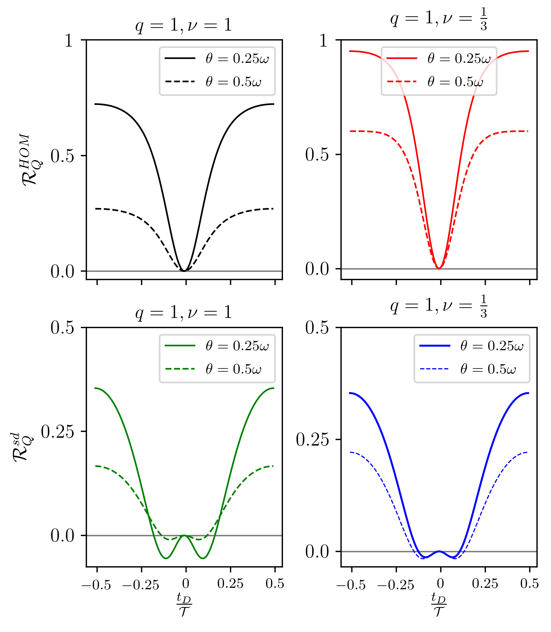
Figure 2: (Color online) HOM heat ratio $\mathcal{R}_{Q}^{HOM}$ (upper panels) and single-drive heat ratio $\mathcal{R}_{Q}^{sd}$ (lower panels) as a function of the time delay $t_{D}$ for $q=1$ and temperatures $\theta=0.25\omega$ (solid lines) and $\theta=0.5\omega$ (dashed lines). The integer case (left panel) and the fractional case for $\nu=\frac{1}{3}$ (right panel) are compared. The other parameters are $W=0.1\mathcal{T}$ and $\omega=0.01\omega_{c}$.

In the following, we exploit the full generality of our derivation by performing the analysis for different values of $q$.
We start by considering the regime where thermal and quantum fluctuations are comparable.
As a beginning, we focus on the relevant case of $q=1$, where states formed by a single leviton are injected from both sources Moskalets and Haack (2017). The collision of identical single-leviton states is very interesting because previous work on fluctuations of charge current proved that in this case the ratio of HOM charge noise is independent of filling factors and temperatures, acquiring an universal analytical expression Rech et al. (2017); Glattli and Roulleau (2016). In order to perform a similar comparison for the heat noise, we present in Fig. 2 the HOM heat ratio (upper panels) considering two temperatures $\theta=0.25\omega$ (solid line) and $\theta=0.5\omega$ (dashed lines) for both the integer and fractional case. Contrarily to the charge case, these curves are all clearly distinct. This means that this universality does not extend also to heat fluctuations. This fact can be explained by the dependence of heat HOM noise on the energy distribution of particles injected by the drives, which in turn is significantly affected by the temperature and by the strength of correlations encoded in the filling factor $\nu$. In particular, as the temperature is further increased, the thermal fluctuations tend to hide the effect of the voltages, resulting in a reduction of $\mathcal{R}_{Q}^{HOM}$ for both filling factors.
Interestingly, we also note that the single-drive ratio can switch sign as $t_{D}$ is tuned, independently of the filling factor. Since $\mathcal{S}_{Q}^{R}$ is independent of $t_{D}$, the change of sign of $\mathcal{R}_{Q}^{sd}$ is entirely due to $\mathcal{S}^{sd}_{Q}$ itself. This is a remarkable difference with respect to the charge noise generated in the same configurations, since charge conservation fixes the sign of current-current correlations. On the contrary, it should be pointed out that the sign of heat noise is not constrained by any conservation law Moskalets (2014).

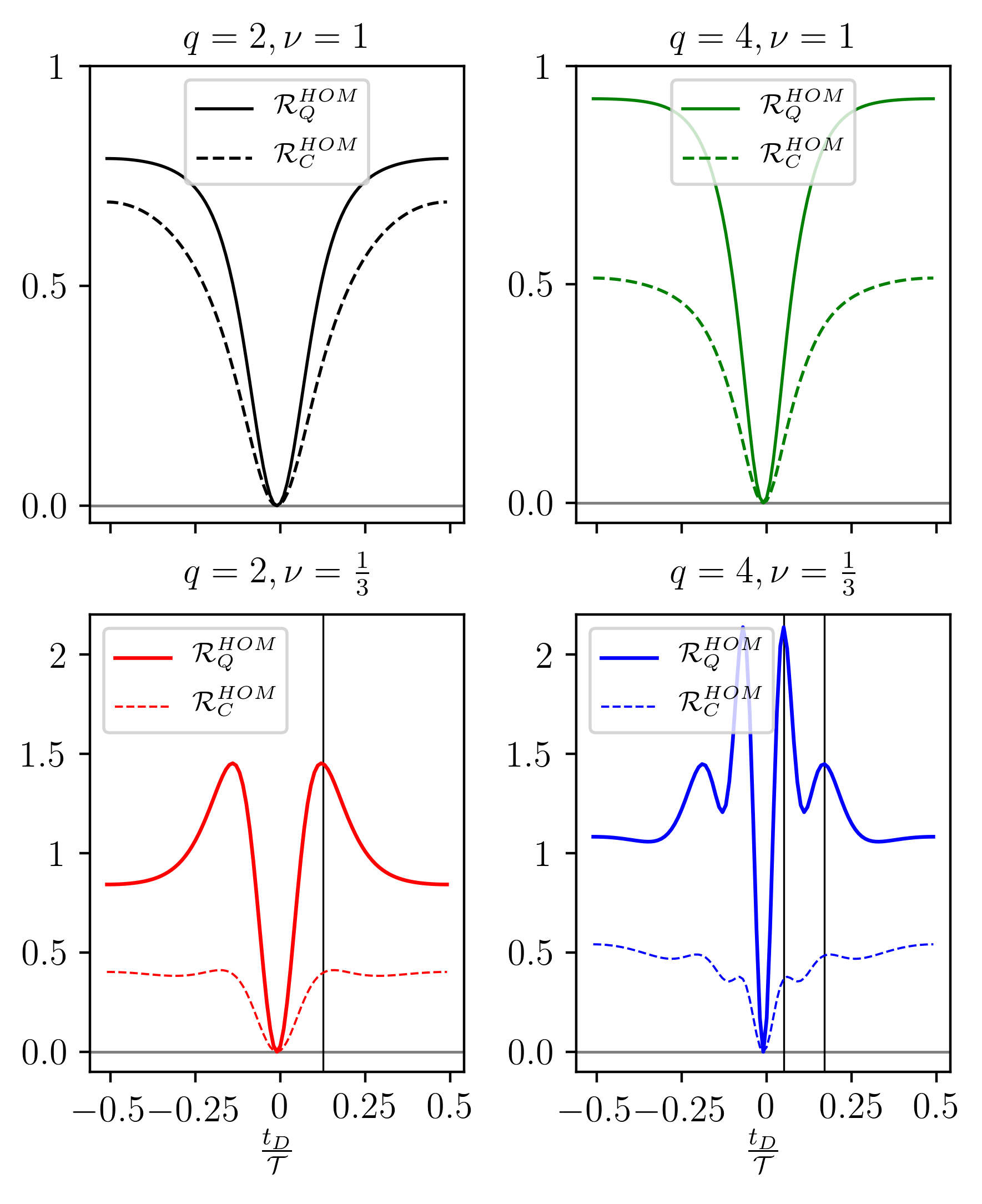
Figure 3: HOM heat ratio $\mathcal{R}_{Q}^{HOM}$ (solid lines) and HOM charge ratio $\mathcal{R}_{C}^{HOM}$ (dashed lines) as a function of the time delay $t_{D}$ for $q=2$ and $q=4$. The integer case (upper panels) and the fractional case for $\nu=\frac{1}{3}$ (lower panels) are compared. Black vertical lines demonstrate the exact correspondence of side peaks appearing in charge and heat ratio. The other parameters are $W=0.1\mathcal{T}$, $\theta=0.25\omega$ and $\omega=0.01\omega_{c}$.

In Fig. 3, we start looking at the collision of states composed by multiple levitons and compare HOM charge and heat ratios (solid and dashed lines, respectively) for $q=2$ and $q=4$. In the fermionic case, presented in the two upper panels, both charge and heat ratio show a single smooth dip at $t_{D}=0$, without additional side features. Interestingly, heat fluctuations are enhanced with respect to charge: in particular, heat HOM ratios saturate to their asymptotic value for smaller values of time delay compared to charge ratio. Again, the enhancement of heat fluctuations can be related to the fact that heat is not constrained by any conservation law, in contrast to the case of charge.
Very remarkably, the curves for the HOM ratio in the fractional case display instead some unexpected side peaks and dips in addition to the central dip. In particular, the number of these maxima and minima increases for states composed with more levitons. A recent paper by the authors explained this intriguing result for charge HOM noise in terms of a crystallization process induced by strong correlation on the charge density of $q$ levitons , i.e. a re-arrangement of the density into an oscillating and ordered pattern with a number of peaks related to $q$ Ronetti et al. (2018). Black vertical lines in the lower panel of Fig. 3 demonstrate the exact correspondence of side peaks appearing in charge and heat ratio as a function of time delay. Based on this argument, we can infer that the HOM heat noise is affected by the crystallization induced in the propagating levitons, thus giving rise to the features observed in the lower panel of Fig. 3. While the oscillating pattern of $\mathcal{R}_{Q}^{HOM}$ remarkably matches with that of $\mathcal{R}_{C}^{HOM}$, the amplitude oscillations are widely enhanced for heat fluctuations, in particular for the peaks occurring at small values of time delay.

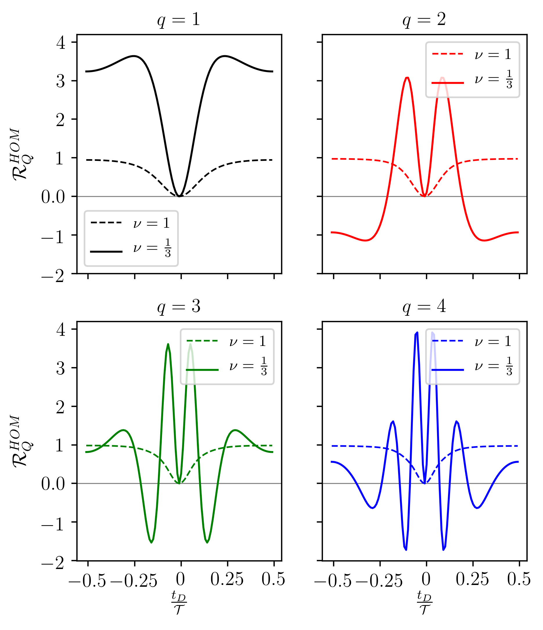
Figure 4: (Color online) HOM heat ratio $\mathcal{R}_{Q}^{HOM}$ as a function of the time delay $t_{D}$ for $q=1$, $q=2$, $q=3$, $q=4$. The integer case (dashed lines) and the fractional case for $\nu=\frac{1}{3}$ (solid lines) are compared. The other parameters are $W=0.1\mathcal{T}$, $\theta=10^{-4}\omega$ and $\omega=0.01\omega_{c}$.

We conclude by noticing that strong correlation of the fractional regime can increase the value of the HOM heat ratio even above $1$. Once again, since this is not the case for the single-drive contribution, this is due to the presence of $\Delta\mathcal{S}_{Q}$, which is peculiar to collision between levitons incoming from different reservoirs.
Now, we consider the regime of very low temperature $\theta\ll\omega$, where the quantum effects should be largely enhanced with respect to the thermal fluctuations. Having established from the previous discussion the connection between $\Delta\mathcal{S}_{Q}$ and $\mathcal{S}_{Q}^{HOM}$ in the fractional regime, we focus only on the HOM heat ratio $\mathcal{R}_{Q}^{HOM}$.
The plots for $\mathcal{R}_{Q}^{HOM}$ in the integer and in the fractional case are compared in Fig. 4 for different values of $q$. In the integer case, a single smooth dip is present for all the values of $q$, confirming the phenomenology described for the finite temperature case. For the strongly correlated case, at $q=1$ one observes a smooth profile, except for a small decrease close to $t_{D}=0.5$. Intriguingly, the oscillations observed in Fig. 3 for $q>1$ are widely enhanced in this regime, such that the HOM ratio displays zeros, whose number increases with $q$, in addition to the central one and can also reach negative values.

V Conclusion

In this work, we investigated charge and heat current fluctuations in an HOM interferometer in the fractional quantum Hall regime. Here, two identical leviton excitations impinge at a QPC with a given time delay. We started by evaluating zero-frequency cross-correlated charge and heat noises in the presence of two generic driving voltage $V_{L}$ and $V_{R}$. We demonstrated that heat noise in this double-drive configuration depends on both $V_{+}=V_{L}+V_{R}$ and $V_{-}=V_{L}-V_{R}$ and, thus, cannot be reproduced in a single-drive setup driven by the voltage $V_{-}$ only. In particular, this implies that single-drive configuration and HOM interferometer implemented with voltage sources are two physically distinct experimental configurations. Moreover, we proved that the HOM heat ratio vanishes for a null time delay for both integer and fractional filling factors, despite the presence, in the latter case, of emergent fractionally charged quasi-particles. Finally, we investigated the form of HOM heat ratio for different regimes of temperatures. Interestingly, unexpected side dips emerged only in the fractional regime which can be related to the crystallization mechanism recently predicted for levitons Ronetti et al. (2018).

Appendix A Coupling to the gate

In this Appendix, we show that there is no gauge transformation able to link the equations of motion for the configurations with two driving voltages $V_{R}$ and $V_{L}$ and the configuration with a single drive $V_{-}=V_{R}-V_{L}$, presented in the main text.
In the double-drive setup a voltage drive is applied both to right-moving and left-moving excitations. We consider a situation in which the vector potentials $\mathcal{A}_{R/L}(x,t)$ are absent. The Lagrangian density is

$$\mathcal{L} =\frac{1}{4\pi}\bigg{\{}-\partial_{x}\Phi_{R}(x,t)\big{[}\partial_{t}\Phi_{R}(x,t)+v\partial_{x}\Phi_{R}(x,t)\big{]}+\partial_{x}\Phi_{L}(x,t)\big{[}\partial_{t}\Phi_{L}(x,t)-v\partial_{x}\Phi_{L}(x,t)\big{]}\bigg{\}}+$$

$$\quad+\frac{e\sqrt{\nu}}{2\pi}\bigg{[}\partial_{x}\Phi_{R}(x,t)\mathcal{V}_{R}(x,t)-\partial_{x}\Phi_{L}(x,t)\mathcal{V}_{L}(x,t)\bigg{]}.$$ (62)

The Euler-Lagrange equations

$$\partial_{t}\frac{\delta\mathcal{L}}{\delta\partial_{t}\Phi_{\alpha}}+\partial_{x}\frac{\delta\mathcal{L}}{\delta\partial_{x}\Phi_{\alpha}}-\frac{\delta\mathcal{L}}{\delta\Phi_{\alpha}}=0$$ (63)

with $\alpha=R,L$, give rise to the following equation of motions for the bosonic fields:

$$(\partial_{t}+v\partial_{x})\Phi_{R}(x,t)=e\sqrt{\nu}\mathcal{V}_{R}(x,t)$$ (64)

$$(\partial_{t}-v\partial_{x})\Phi_{L}(x,t)=e\sqrt{\nu}\mathcal{V}_{L}(x,t).$$ (65)

In order to model the system presented in Sec. II, the form for the voltage drives is

$$\mathcal{V}_{R}(x,t) =f_{R}(x)V_{R}(t)$$ (66)

$$\mathcal{V}_{L}(x,t) =f_{L}(x)V_{L}(t)$$ (67)

where $f_{R/L}(x)$ are time-independent, while $V_{R/L}(t)$ are space-independent. In this case equation of motions for the double-drive setup are

$$(\partial_{t}+v\partial_{x})\Phi_{R}(x,t)=e\sqrt{\nu}f_{R}(x)V_{R}(t)$$ (68a)

$$(\partial_{t}-v\partial_{x})\Phi_{L}(x,t)=e\sqrt{\nu}f_{L}(x)V_{L}(t).$$ (68b)

We also consider a single-drive setup with an effective voltage drive $\mathcal{V}_{R}(x,t)=f_{R}(x)[V_{R}(t)-V_{L}(t)]$ on the right side, and the left side grounded [$\mathcal{V}_{L}(x,t)=0$]. We still consider that the magnetic potential is zero on both edges. It is immediate to show that the equation of motions are now

$$(\partial_{t}+v\partial_{x})\Phi_{R}(x,t)=e\sqrt{\nu}f_{R}(x)[V_{R}(t)-V_{L}(t)]$$ (69a)

$$(\partial_{t}-v\partial_{x})\Phi_{L}(x,t)=0$$ (69b)

A.1 Applying gauge transformations to the HOM setup

Here we show that a gauge transformation that operates in the following way on the voltage drives

$$\begin{cases}\mathcal{V}_{R}(x,t)=f_{R}(x)V_{R}(t)\\ \mathcal{V}_{L}(x,t)=f_{L}(x)V_{L}(t)\end{cases}\longrightarrow\begin{cases}\mathcal{V}^{\prime}_{R}(x,t)=f_{R}(x)[V_{R}(t)-V_{L}(t)]\\ \mathcal{V}^{\prime}_{L}(x,t)=0,\end{cases}$$ (70)

does not transform Eqs. (68) into Eqs. (69), but leaves them unchanged.
We recall that a general gauge transformation that leaves invariant an electromagnetic field is given by

$$\mathcal{V}^{\prime}_{R/L}(x,t) =\mathcal{V}_{R/L}(x,t)-\partial_{t}\chi_{R}(x,t),$$ (71)

$$\mathcal{A}^{\prime}_{R/L}(x,t) =\mathcal{A}_{R/L}(x,t)+\partial_{x}\chi_{R}(x,t),$$ (72)

with $\chi_{R/L}(x,t)$ a scalar function.
In our particular case, voltage potentials are required to transform as

$$\mathcal{V}^{\prime}_{R}(x,t) =f_{R}(x)V_{R}(x)-\partial_{t}\chi_{R}(x,t)=f_{R}(x)[V_{R}(t)-V_{L}(t)]$$ (73)

$$\mathcal{V}^{\prime}_{L}(x,t) =f_{L}(x)V_{L}(x)-\partial_{t}\chi_{L}(x,t)=0$$ (74)

for the right-moving and left-moving sector respectively. The transformation is evidently implemented by the choice

$$\chi_{R}(x,t) =f_{R}(x)\int_{0}^{t}d\tau V_{L}(\tau)$$ (75a)

$$\chi_{L}(x,t) =f_{L}(x)\int_{0}^{t}d\tau V_{L}(\tau)$$ (75b)

Since these equations involve spatial-dependent functions, we expect that non-zero magnetic potentials arise as a consequence of the gauge transformation. In the new gauge we get non-zero magnetic potentials given by (in our initial gauge choice $\mathcal{A}_{R/L}=0$)

$$\mathcal{A}^{\prime}_{R}(x,t) =\partial_{x}f_{R}(x)\int_{0}^{t}d\tau V_{L}(\tau)$$ (76)

$$\mathcal{A}^{\prime}_{L}(x,t) =\partial_{x}f_{L}(x)\int_{0}^{t}d\tau V_{L}(\tau)$$ (77)

and the Lagrangian density now reads

$$\mathcal{L}^{\prime} =\frac{1}{4\pi}\bigg{\{}-\partial_{x}\Phi_{R}(x,t)\big{[}\partial_{t}\Phi_{R}(x,t)+v\partial_{x}\Phi_{R}(x,t)\big{]}+\partial_{x}\Phi_{L}(x,t)\big{[}\partial_{t}\Phi_{L}(x,t)-v\partial_{x}\Phi_{L}(x,t)\big{]}\bigg{\}}+$$

$$\quad+\frac{e\sqrt{\nu}}{2\pi}\bigg{\{}\partial_{x}\Phi_{R}(x,t)f_{R}(x)[V_{R}(t)-V_{L}(t)]+\big{[}\partial_{t}\Phi_{R}(x,t)\partial_{x}f_{R}(x)-\partial_{t}\Phi_{L}(x,t)\partial_{x}f_{L}(x)\big{]}\int_{t_{0}}^{t}d\tau V_{L}(\tau)\bigg{\}}$$ (78)

where the last term accounts for the presence of $\mathcal{A}^{\prime}_{R}(x,t)$ and $\mathcal{A}^{\prime}_{L}(x,t)$. We now look for the equation of motions in this new configuration. From Euler-Lagrange equations one gets

$$(\partial_{t}+v\partial_{x})\Phi_{R}(x,t)=$$

$$=e\sqrt{\nu}f_{R}(x)[V_{R}(t)-V_{L}(t)]+e\sqrt{\nu}f_{R}(x)V_{L}(t)=$$

$$=e\sqrt{\nu}f_{R}(x)V_{R}(t)$$ (79)

$$(\partial_{t}-v\partial_{x})\Phi_{L}(x,t)=e\sqrt{\nu}f_{L}(x)V_{L}(t).$$ (80)

Note that we have not recovered the equation of motions for the single drive setup, Eqs. (69), as one may naively expect. On the contrary, we have found the equations of motion for the double-drive setup, Eqs. (68).

Appendix B Heat noise

In this Appendix, we give more details about the calculation of heat noise presented in Sec. III. Before starting with the derivation of heat noise, we would give some formulas that would be useful in the following parts.

B.1 Useful formulas

In the following, we derive some results that would be useful for the evaluation of heat current fluctuations. In particular, our goal is to evaluate the following average values (for simplicity, we drop all the low indices $R$ or $L$)

$$C_{1}(t_{1},t_{2},t_{3})=\langle\partial_{t_{1}}\phi(t_{1})e^{i\sqrt{\nu}\phi(t_{2})}e^{-i\sqrt{\nu}\phi(t_{3})}\rangle,$$ (81)

$$C_{2}(t_{1},t_{2},t_{3})=\langle e^{i\sqrt{\nu}\phi(t_{1})}e^{-i\sqrt{\nu}\phi(t_{2})}\partial_{t_{3}}\phi(t_{3})\rangle,$$ (82)

$$D_{1}(t_{1},t_{2},t_{3})=\langle\left(\partial_{t_{1}}\phi(t_{1})\right)^{2}e^{i\sqrt{\nu}\phi(t_{2})}e^{-i\sqrt{\nu}\phi(t_{3})}\rangle,$$ (83)

$$D_{2}(t_{1},t_{2},t_{3})=\langle e^{i\sqrt{\nu}\phi(t_{1})}e^{-i\sqrt{\nu}\phi(t_{2})}\left(\partial_{t_{3}}\phi(t_{3})\right)^{2}\rangle,$$ (84)

where the thermal average is performed over the initial equilibrium density matrix, in absence of tunneling and driving voltage and bosonic fields evolve according to the edge Hamiltonian $H_{0}$. In order to evaluate $C_{1}$ and $C_{2}$, we start by considering the following general average value

$$E_{1}(\epsilon_{1},\epsilon_{2},\epsilon_{3};t_{1},t_{2},t_{3})=\langle e^{-i\epsilon_{1}\phi(t_{1})}e^{-i\epsilon_{2}\phi(t_{2})}e^{-i\epsilon_{3}\phi(t_{3})}\rangle,$$ (85)

which is connected to $C_{1}$ and $C_{2}$ by this relation

$$C_{1}(t_{1},t_{2},t_{3})=i\partial_{t_{1}}\left\{\lim\limits_{\epsilon_{1}\rightarrow 0}\partial_{\epsilon_{1}}E_{1}(\epsilon_{1},\epsilon_{2},\epsilon_{3};t_{1},t_{2},t_{3})\right\}_{\begin{subarray}{c}\epsilon_{2}=-\sqrt{\nu}\\ \epsilon_{3}=\sqrt{\nu}\end{subarray}},$$ (86)

$$C_{2}(t_{1},t_{2},t_{3})=i\partial_{t_{3}}\left\{\lim\limits_{\epsilon_{3}\rightarrow 0}\partial_{\epsilon_{3}}E_{1}(\epsilon_{1},\epsilon_{2},\epsilon_{3};t_{1},t_{2},t_{3})\right\}_{\begin{subarray}{c}\epsilon_{1}=-\sqrt{\nu}\\ \epsilon_{2}=\sqrt{\nu}\end{subarray}}.$$ (87)

By using von Delft and Schoeller (1998)

$$\langle e^{\chi(t_{1})}e^{\chi(t_{2})}e^{\chi(t_{3})}\rangle=e^{\frac{1}{2}\sum_{i=1}^{3}\langle\chi(t_{i})^{2}\rangle}e^{\sum_{i<j}\langle\chi(t_{i})\chi(t_{j})\rangle},$$ (88)

we obtain from Eq. (85)

$$E_{1}(\epsilon_{1},\epsilon_{2},\epsilon_{3};x_{1},x_{2},x_{3})=e^{-\frac{1}{2}\sum_{i=1}^{3}\langle\epsilon_{i}^{2}\phi^{2}(x_{i})\rangle}\times$$

$$\times e^{-\left\{\epsilon_{1}\epsilon_{2}\langle\phi(x_{1})\phi(x_{2})\rangle+\epsilon_{1}\epsilon_{3}\langle\phi(x_{1})\phi(x_{3})\rangle+\epsilon_{2}\epsilon_{3}\langle\phi(x_{2})\phi(x_{3})\rangle\right\}}.$$ (89)

Finally, we use Eqs. (86) and (87) to find $C_{1}$ and $C_{2}$

$$C_{1}(t_{1},t_{2},t_{3}) =-i\sqrt{\nu}\mathcal{K}(t_{1},t_{2},t_{3})P_{\nu}(t_{2}-t_{3}),$$ (90)

$$C_{2}(t_{1},t_{2},t_{3}) =-i\sqrt{\nu}\mathcal{K}(-t_{3},-t_{1},-t_{2})P_{\nu}(t_{1}-t_{2}),$$ (91)

where we defined (see Eq. (19) in the main text)

$$P_{g}(t^{\prime}-t) =\langle e^{i\sqrt{g}\phi_{R/L}(0,t^{\prime})}e^{-i\sqrt{g}\phi_{R/L}(0,t)}\rangle=$$

$$=\left[\frac{\pi\theta\tau}{\sinh\left(\pi\theta\tau\right)\left(1+i\omega_{c}\tau\right)}\right]^{g},$$ (92)

and

$$\mathcal{K}(t_{1},t_{2},t_{3}) =\partial_{t_{1}}\left\{\langle\phi(t_{1})\phi(t_{3})\rangle-\langle\phi(t_{1})\phi(t_{2})\rangle\right\}=$$

$$=\int d\tau\mathcal{P}_{2}(t_{1}-\tau)\left(\Theta(\tau-t_{3})-\Theta(\tau-t_{2})\right).$$ (93)

One could also obtain the following similar relations

$$\langle\partial_{t_{1}}\phi(t_{1})e^{-i\sqrt{\nu}\phi(t_{2})}e^{i\sqrt{\nu}\phi(t_{3})}\rangle=i\sqrt{\nu}\mathcal{K}(t_{1},t_{2},t_{3})P_{\nu}(t_{2}-t_{3}),$$ (94)

$$\langle e^{-i\sqrt{\nu}\phi(t_{1})}e^{i\sqrt{\nu}\phi(t_{2})\partial_{t_{3}}\phi(t_{3})}\rangle=i\sqrt{\nu}\mathcal{K}(-t_{3},-t_{1},-t_{2})P_{\nu}(t_{1}-t_{2}).$$ (95)

Exploiting the following average

$$\langle\partial_{t_{1}}\phi(t_{1})\partial_{t}\phi(t)\rangle=-\frac{\pi^{2}\theta^{2}}{v^{2}\sinh^{2}\left(\pi\theta(t_{1}-t)\right)}$$ (96)

the function $\mathcal{K}$ can be further evaluated by using

$$\partial_{t_{1}}\langle\phi(t_{1})\phi(t_{2})\rangle =\int_{-\infty}^{t_{2}}dt\langle\partial_{t_{1}}\phi(t_{1})\partial_{t}\phi(t)\rangle=$$

$$=\frac{\pi\theta}{v}\left[\coth\left(\pi\theta(t_{1}-t_{2})\right)-1\right].$$ (97)

By using this result, one finds

$$\mathcal{K}(t_{1},t_{2},t_{3} )=\frac{\pi\theta}{v}\left(\coth\left(\pi\theta(t_{1}-t_{3})\right)-\coth\left(\pi\theta(t_{1}-t_{2})\right)\right)=$$

$$= \frac{\pi\theta}{v}\frac{\sinh\left(\pi\theta(t_{2}-t_{3})\right)}{\sinh\left(\pi\theta(t_{1}-t_{3})\right)\sinh\left(\pi\theta(t_{1}-t_{2})\right)}.$$ (98)

In order to evaluate $D_{1}$ and $D_{2}$, we start by considering the following general average value

$$E_{2}(\epsilon_{1},\epsilon_{2},\epsilon_{3},\epsilon_{4};t_{1},t_{2},t_{3},t_{4})=$$

$$=\langle e^{-i\epsilon_{1}\phi(t_{1})}e^{-i\epsilon_{2}\phi(t_{2})}e^{-i\epsilon_{3}\phi(t_{3})}e^{-i\epsilon_{4}\phi(t_{4})}\rangle,$$ (99)

which is connected to $D_{1}$ and $D_{2}$ by these relations

$$D_{1}(t_{1},t_{2},t_{3}) =-\partial_{t_{1}}\partial_{t^{\prime}_{1}}\left\{\lim\limits_{\epsilon_{1}\rightarrow 0,\epsilon_{2}\rightarrow 0}\partial_{\epsilon_{1}}\partial_{\epsilon_{2}}E_{2}(\epsilon_{1},\epsilon_{2},\epsilon_{3},\epsilon_{4};t_{1},t^{\prime}_{1},t_{2},t_{3})\right\}_{\begin{subarray}{c}\epsilon_{1}=-\epsilon_{2}=-\sqrt{\nu}\\ t^{\prime}_{1}=t_{1}\end{subarray}},$$ (100)

$$D_{2}(t_{1},t_{2},t_{3}) =-\partial_{t_{3}}\partial_{t^{\prime}_{3}}\left\{\lim\limits_{\epsilon_{1}\rightarrow 0,\epsilon_{2}\rightarrow 0}\partial_{\epsilon_{3}}\partial_{\epsilon_{4}}E_{2}(\epsilon_{1},\epsilon_{2},\epsilon_{3},\epsilon_{4};t_{1},t_{2},t_{3},t^{\prime}_{3})\right\}_{\begin{subarray}{c}\epsilon_{4}=-\epsilon_{3}=\sqrt{\nu}\\ t^{\prime}_{3}=t_{3}\end{subarray}},$$ (101)

By using Eq. (88), we obtain from Eq. (85)

$$E_{2}(\epsilon_{1},\epsilon_{2},\epsilon_{3},\epsilon_{4};t_{1},t_{2},t_{3},t_{4})=e^{-\frac{1}{2}\sum_{i=1}^{4}\epsilon_{i}^{2}\langle\phi^{2}(t_{i})\rangle}\cdot$$ (103)

$$\cdot e^{-\left\{\epsilon_{1}\epsilon_{2}\langle\phi(t_{1})\phi(t_{2})\rangle+\epsilon_{1}\epsilon_{3}\langle\phi(t_{1})\phi(t_{3})\rangle+\epsilon_{1}\epsilon_{4}\langle\phi(t_{1})\phi(t_{4})\rangle+\epsilon_{2}\epsilon_{3}\langle\phi(t_{2})\phi(t_{3})\rangle+\epsilon_{2}\epsilon_{4}\langle\phi(t_{2})\phi(t_{4})\rangle+\epsilon_{3}\epsilon_{4}\langle\phi(t_{3})\phi(t_{4})\rangle\right\}}.$$ (104)

Finally, we use Eq. (100) and (101) to find $D_{1}$ and $D_{2}$

$$\left(\partial_{t_{1}}\phi(t_{1})\right)^{2}e^{i\sqrt{\nu}\phi(t_{2})}e^{-i\sqrt{\nu}\phi(t_{3})}\rangle =\left\{\langle\left(\partial_{t_{1}}\phi(t_{1})\right)^{2}\rangle-\nu\left(\mathcal{K}(t_{1},t_{2},t_{3})\right)^{2}\right\}P_{\nu}(t_{2}-t_{3}),$$ (105)

$$\hskip 5.69054pt\langle e^{i\sqrt{\nu}\phi(t_{1})}e^{-i\sqrt{\nu}\phi(t_{2})}\left(\partial_{t_{3}}\phi(t_{3})\right)^{2}\rangle =\left\{\langle\left(\partial_{t_{3}}\phi(t_{3})\right)^{2}\rangle-\nu\left(\mathcal{K}(-t_{3},-t_{1},-t_{2})\right)^{2}\right\}P_{\nu}(t_{1}-t_{2}).$$ (106)

By carrying on a similar calculation, one can find also the analogous quantities

$$\left(\partial_{t_{1}}\phi(t_{1})\right)^{2}e^{-i\sqrt{\nu}\phi(t_{2})}e^{i\sqrt{\nu}\phi(t_{3})}\rangle =\left\{\langle\left(\partial_{t_{1}}\phi(t_{1})\right)^{2}\rangle-\nu\left(\mathcal{K}(t_{1},t_{2},t_{3})\right)^{2}\right\}P_{\nu}(t_{2}-t_{3}),$$ (107)

$$\hskip 5.69054pt\langle e^{-i\sqrt{\nu}\phi(t_{1})}e^{i\sqrt{\nu}\phi(t_{2})}\left(\partial_{t_{3}}\phi(t_{3})\right)^{2}\rangle =\left\{\langle\left(\partial_{t_{3}}\phi(t_{3})\right)^{2}\rangle-\nu\left(\mathcal{K}(-t_{3},-t_{1},-t_{2})\right)^{2}\right\}P_{\nu}(t_{1}-t_{2}).$$ (108)

B.2 Calculations of heat noise

Our starting point is the perturbative expression of heat noise given in the main text (see Eq. (25))

$$\mathcal{S}_{Q}=\mathcal{S}_{Q}^{(02)}+\mathcal{S}_{Q}^{(20)}+\mathcal{S}_{Q}^{(11)}+\mathcal{O}\left(\left|\Lambda\right|^{3}\right).$$ (109)

Firstly, we derive the term $\mathcal{S}_{Q}^{(11)}$, which reads

$$\mathcal{S}_{Q}^{(11)} =\int_{0}^{\mathcal{T}}\frac{dt}{\mathcal{T}}\int dt^{\prime}\Big{\{}\langle\partial_{t^{\prime}}\Psi^{\dagger}_{R}(0,t^{\prime})\Psi_{L}(0,t^{\prime})\partial_{t}\Psi^{\dagger}_{L}(0,t)\Psi_{R}(0,t)\rangle+$$

$$+\langle\Psi^{\dagger}_{L}(0,t^{\prime})\partial_{t^{\prime}}\Psi_{R}(0,t^{\prime})\Psi^{\dagger}_{R}(0,t)\partial_{t}\Psi_{L}(0,t)\rangle\Big{\}},$$ (110)

since $\langle\mathcal{J}_{2/3}^{(1)}(t)\rangle=0$ (see Eq. (33) in the main text). We recall that the time evolution of quasi-particle fields is

$$\Psi_{R,L}(x,t)=\frac{\mathcal{F}_{R/L}}{\sqrt{2\pi a}}e^{-i\sqrt{\nu}\phi_{R/L}(x,t)}e^{i\nu e\int_{t_{0}}^{t\mp\frac{x}{v}-\frac{d}{v}}dt^{\prime}V_{R/L}(t^{\prime})}.$$ (111)

We can further express the average in the above equation as

$$\mathcal{S}_{Q}^{(11)}=2\left|\lambda\right|^{2}\int_{0}^{\mathcal{T}}\frac{dt}{\mathcal{T}}\int dt^{\prime}\hskip 2.84526pt\Big{\{}\cos{\left(\nu e\int_{t^{\prime}}^{t}dt^{\prime\prime}V_{R}(t^{\prime\prime})-V_{L}(t^{\prime\prime})\right)}\partial_{t}^{\prime}\mathcal{P}_{\nu}(t^{\prime}-t)\partial_{t}\mathcal{P}_{\nu}(t^{\prime}-t)+$$ (112)

$$+\nu eV_{R}(t^{\prime})\sin{\left(\nu e\int_{t^{\prime}}^{t}dt^{\prime\prime}V_{R}(t^{\prime\prime})-V_{L}(t^{\prime\prime})\right)}\frac{1}{2}\partial_{t}\mathcal{P}_{2\nu}(t^{\prime}-t)+\nu eV_{L}(t)\sin{\left(\nu e\int_{t^{\prime}}^{t}dt^{\prime\prime}V_{R}(t^{\prime\prime})-V_{L}(t^{\prime\prime})\right)}\frac{1}{2}\partial_{t^{\prime}}\mathcal{P}_{2\nu}(t^{\prime}-t)+$$

$$-\nu^{2}e^{2}V_{R}(t^{\prime})V_{L}(t)\cos{\left(\nu e\int_{t^{\prime}}^{t}dt^{\prime\prime}V_{R}(t^{\prime\prime})-V_{L}(t^{\prime\prime})\right)}\mathcal{P}_{2\nu}(t^{\prime}-t)\Big{\}}\leavevmode\nobreak\ ,$$

where the function $P_{g}(t)$ is defined in Eq. (B.1) and $\lambda\equiv\frac{\Lambda}{2\pi a}$. The integration by parts of second and third line of Eq. (112) provides some useful eliminations, providing the final expression for this contribution

$$\mathcal{S}_{Q}^{(11)}=2\left|\lambda\right|^{2}\int_{0}^{\mathcal{T}}\frac{dt}{\mathcal{T}}\int dt^{\prime}\hskip 2.84526pt\Big{\{}\cos{\left(\nu e\int_{t^{\prime}}^{t}dt^{\prime\prime}\left(V_{R}(t^{\prime\prime})-V_{L}(t^{\prime\prime})\right)\right)}\partial_{t}^{\prime}\mathcal{P}_{\nu}(t^{\prime}-t)\partial_{t}\mathcal{P}_{\nu}(t^{\prime}-t)+$$ (113)

$$-\frac{1}{2}\nu^{2}e^{2}\left(V_{R}(t^{\prime})V_{R}(t)+V_{L}(t^{\prime})V_{L}(t)\right)\cos{\left(\nu e\int_{t^{\prime}}^{t}dt^{\prime\prime}\left(V_{R}(t^{\prime\prime})-V_{L}(t^{\prime\prime})\right)\right)}\mathcal{P}_{2\nu}(t^{\prime}-t)\Big{\}}\leavevmode\nobreak\ .$$ (114)

We focus on the remaining contributions, starting from $\mathcal{S}_{Q}^{(02)}$: the calculations for the other term would be analogous. By plugging Eqs. (26) and (28) in the definition of $\mathcal{S}_{Q}^{(02)}$, one finds

$$\mathcal{S}_{Q}^{(02)} =-i\frac{\left|\lambda\right|^{2}}{4\pi}\int dt\int_{0}^{\mathcal{T}}\frac{dt^{\prime}}{\mathcal{T}}\int dt^{\prime\prime}\theta(t^{\prime}-t^{\prime\prime})\Big{\{}\langle\left(\partial_{t}\phi_{R}(0,t)\right)^{2}\left[\Psi^{\dagger}_{R}(0,t^{\prime\prime})\Psi_{L}(0,t^{\prime\prime}),\partial_{t^{\prime}}\Psi^{\dagger}_{L}(0,t^{\prime})\Psi_{R}(0,t^{\prime})\right]\rangle+$$

$$-2\nu eV_{R}(t)\langle\partial_{t}\phi_{R}(0,t)\left[\Psi^{\dagger}_{R}(0,t^{\prime\prime})\Psi_{L}(0,t^{\prime\prime}),\partial_{t^{\prime}}\Psi^{\dagger}_{L}(0,t^{\prime})\Psi_{R}(0,t^{\prime})\right]\rangle+$$

$$-\langle\left(\partial_{t}\phi_{R}(0,t)\right)^{2}\rangle\langle\left[\Psi^{\dagger}_{R}(0,t^{\prime\prime})\Psi_{L}(0,t^{\prime\prime}),\partial_{t^{\prime}}\Psi^{\dagger}_{L}(0,t^{\prime})\Psi_{R}(0,t^{\prime})\right]\rangle\Big{\}}.$$ (115)

The averages involving the commutators can be performed by using the expression in Eq. (18) for the time evolution of quasi-particle fields and by resorting to the formulas in Eqs (90), (94),(105) and (106) derived in the Appendix B.1. Indeed, one finds

$$\mathcal{S}^{(02)}_{(Q)}=-i\frac{\left|\lambda\right|^{2}}{4\pi}\int dt\int_{0}^{\mathcal{T}}\frac{dt^{\prime}}{\mathcal{T}}\int dt^{\prime\prime}\leavevmode\nobreak\ \Theta\left(t^{\prime}-t^{\prime\prime}\right)\Big{\{}-\Big{[}\nu\partial_{t^{\prime}}\mathcal{K}^{2}(t,t^{\prime},t^{\prime\prime})\cos{\left(\nu e\int_{t^{\prime\prime}}^{t^{\prime}}d\tau V_{-}(\tau)\right)}\left(\mathcal{P}_{2\nu}(t^{\prime\prime}-t^{\prime})-\mathcal{P}_{2\nu}(t^{\prime}-t^{\prime\prime})\right)+$$

$$+\nu eV_{L}(t^{\prime})\mathcal{K}^{2}(t,t^{\prime},t^{\prime\prime})\left(\mathcal{P}_{2\nu}(t^{\prime\prime}-t^{\prime})-\mathcal{P}_{2\nu}(t^{\prime}-t^{\prime\prime})\right)\sin\left({\nu e\int_{t^{\prime\prime}}^{t^{\prime}}d\tau V_{-}(\tau)}\right)\Big{]}+$$

$$+\mathcal{K}(t,t^{\prime},t^{\prime\prime})\Big{[}2\nu eV_{R}(t)\sin\left({\nu e\int_{t^{\prime\prime}}^{t^{\prime}}d\tau V_{-}(\tau)}\right)\partial_{t^{\prime}}\left[\mathcal{P}_{2\nu}\left(t^{\prime\prime}-t^{\prime}\right)-\mathcal{P}_{2\nu}\left(t^{\prime}-t^{\prime\prime}\right)\right]+$$

$$-4\nu^{2}e^{2}V_{R}(t)V_{L}(t^{\prime})\cos\left({\nu e\int_{t^{\prime\prime}}^{t^{\prime}}d\tau V_{-}(\tau)}\right)\left[\mathcal{P}_{2\nu}\left(t^{\prime\prime}-t^{\prime}\right)-\mathcal{P}_{2\nu}\left(t^{\prime}-t^{\prime\prime}\right)\right]\Big{]}\Big{\}},$$

A similar calculation leads to the expression for the last contribution, given by

$$\mathcal{S}^{(20)}_{(Q)}=-i\frac{\left|\lambda\right|^{2}}{4\pi}\int dt\int_{0}^{\mathcal{T}}\frac{dt^{\prime}}{\mathcal{T}}\int dt^{\prime\prime}\leavevmode\nobreak\ \Theta\left(t^{\prime}-t^{\prime\prime}\right)\Big{\{}\Big{[}\nu\partial_{t^{\prime}}\mathcal{K}^{2}(t,t^{\prime},t^{\prime\prime})\cos{\left(\nu e\int_{t^{\prime\prime}}^{t^{\prime}}d\tau V_{-}(\tau)\right)}\left(\mathcal{P}_{2\nu}(t^{\prime\prime}-t^{\prime})-\mathcal{P}_{2\nu}(t^{\prime}-t^{\prime\prime})\right)+$$

$$+\nu eV_{L}(t^{\prime})\mathcal{K}^{2}(t,t^{\prime},t^{\prime\prime})\left(\mathcal{P}_{2\nu}(t^{\prime\prime}-t^{\prime})-\mathcal{P}_{2\nu}(t^{\prime}-t^{\prime\prime})\right)\sin\left({\nu e\int_{t^{\prime\prime}}^{t^{\prime}}d\tau V_{-}(\tau)}\right)\Big{]}+$$

$$+\mathcal{K}(t,t^{\prime\prime},t^{\prime})\Big{[}2\nu eV_{L}(t)\sin\left({\nu e\int_{t^{\prime\prime}}^{t^{\prime}}d\tau V_{-}(\tau)}\right)\partial_{t^{\prime}}\left[\mathcal{P}_{2\nu}\left(t^{\prime\prime}-t^{\prime}\right)-\mathcal{P}_{2\nu}\left(t^{\prime}-t^{\prime\prime}\right)\right]+$$

$$+4\nu^{2}e^{2}V_{R}(t)V_{L}(t^{\prime\prime})\cos\left({\nu e\int_{t^{\prime\prime}}^{t^{\prime}}d\tau V_{-}(\tau)}\right)\left[\mathcal{P}_{2\nu}\left(t^{\prime\prime}-t^{\prime}\right)-\mathcal{P}_{2\nu}\left(t^{\prime}-t^{\prime\prime}\right)\right]\Big{]}\Big{\}}.$$

By summing up the two contributions, one can see that the first lines cancel out and the remaining two lines add up in a way that allows to get rid of the function $\Theta(t^{\prime}-t^{\prime\prime})$, thus obtaining

$$\mathcal{S}^{(02)}_{(Q)}+\mathcal{S}^{(20)}_{(Q)}=-i\frac{\left|\lambda\right|^{2}}{4\pi}\int dt\int_{0}^{\mathcal{T}}\frac{dt^{\prime}}{\mathcal{T}}\int dt^{\prime\prime}\leavevmode\nobreak\ \Big{\{}\mathcal{K}(t,t^{\prime\prime},t^{\prime})\Big{[}2\nu eV_{-}(t)\sin\left({\nu e\int_{t^{\prime\prime}}^{t^{\prime}}d\tau V_{-}(\tau)}\right)\partial_{t^{\prime}}\left[\mathcal{P}_{2\nu}\left(t^{\prime\prime}-t^{\prime}\right)-\mathcal{P}_{2\nu}\left(t^{\prime}-t^{\prime\prime}\right)\right]+$$

$$-4\nu^{2}e^{2}V_{R}(t)V_{L}(t^{\prime\prime})\cos\left({\nu e\int_{t^{\prime\prime}}^{t^{\prime}}d\tau V_{-}(\tau)}\right)\left[\mathcal{P}_{2\nu}\left(t^{\prime\prime}-t^{\prime}\right)-\mathcal{P}_{2\nu}\left(t^{\prime}-t^{\prime\prime}\right)\right]\Big{]}\Big{\}}.$$

Now, summing all the contributions according to Eq. (37), it is possible to obtain the result presented in the main text, which reads

$$\mathcal{S}_{Q}(V_{R},V_{L})=\mathcal{S}_{Q}(V_{-},0)+\Delta\mathcal{S}_{Q}(V_{R},V_{L}),$$ (116)

with

$$\mathcal{S}_{Q}(V_{-},0) =|\lambda|^{2}\int_{0}^{\mathcal{T}}\frac{dt}{\mathcal{T}}\int dt^{\prime}\Big{\{}\cos\left(\nu e\int_{t}^{t^{\prime}}d\tau V_{-}(\tau)\right)\Re\left[\mathcal{P}_{\nu}(t^{\prime}-t)\partial_{t}^{2}\mathcal{P}_{\nu}(t^{\prime}-t)\right]+$$

$$+\frac{\nu ev}{\pi}\int dt^{\prime\prime}V_{-}(t^{\prime})\mathcal{K}\left(t^{\prime},t,t^{\prime\prime}\right)\sin\left(\nu e\int_{t}^{t^{\prime}}d\tau V_{-}(\tau)\right)\Im\left[\partial_{t^{\prime\prime}}\mathcal{P}_{2\nu}(t^{\prime\prime}-t)\right]\Big{\}},$$ (117)

$$\Delta\mathcal{S}_{Q}(V_{R},V_{L}) =\nu^{2}e^{2}|\lambda|^{2}\int_{0}^{\mathcal{T}}\frac{dt}{\mathcal{T}}\int dt^{\prime}\cos\left(\nu e\int_{t}^{t^{\prime}}d\tau V_{-}(\tau)\right)\Big{(}\alpha_{RL}(t,t^{\prime})\Re\left[\mathcal{P}_{2\nu}(t^{\prime}-t)\right]+\beta_{RL}(t,t^{\prime})\Im\left[\mathcal{P}_{2\nu}(t^{\prime}-t)\right]\Big{)},$$ (118)

where we defined the following functions

$$\alpha_{RL}(t,t^{\prime})=\left(V_{R}(t)V_{L}(t^{\prime})-V_{L}(t)V_{R}(t^{\prime})\right),$$ (119)

$$\beta_{RL}=\frac{v}{\pi}\int dt^{\prime\prime}\mathcal{K}(t^{\prime\prime},t,t^{\prime})V_{R}(t^{\prime\prime})\left[V_{L}(t^{\prime})-V_{L}(t)\right].$$ (120)

Appendix C Fourier coefficients

This Appendix is devoted to the Fourier analysis of the Lorentzian periodic signal $V_{Lor}(t)$ and of the phase $e^{-i\nu e\int_{t_{0}}^{t}dt^{\prime}V_{Lor}(t^{\prime})}$, where

$$V_{Lor}(t) =\frac{V_{0}}{\pi}\sum_{k=-\infty}^{+\infty}\frac{W}{W^{2}+(t-k\mathcal{T})^{2}},$$ (121)

where $\mathcal{T}$ is the periodic, $V_{0}$ the amplitude and $W$ the half width at half maximum.
The coefficients for the Fourier series of the expression $\nu eV_{Lor}(t)=\sum_{k}c_{k}e^{ik\omega t}$ are

$$c_{k}=q\omega e^{-2\pi\frac{W}{\mathcal{T}}|k|},$$ (122)

with $q=\frac{\nu e}{2\pi}\int_{0}^{\mathcal{T}}dtV_{Lor}(t)=\frac{\nu eV_{0}}{\omega}$.
We also note that, for the time delayed voltage $V_{Lor}(t+t_{D})$, the coefficients become $c^{\prime}_{k}=c_{k}e^{-ik\omega t_{D}}$.
The Fourier series $e^{-i\nu e\int_{0}^{t}dt^{\prime}(V_{Lor}(t^{\prime})-V_{0})}=\sum_{l}p_{l}e^{-il\omega t}$ allows to deal with the time-dependent problem as a superposition of time-independent configurations, with energy shifted by an integer amount of energy quanta $\omega$. For the Lorentzian case, it is convenient to switch to a complex representation in terms of the variable $z=e^{i\omega t}$. After some algebra and introducing $\gamma=e^{-2\pi\eta}$ one finds Dubois et al. (2013a); Grenier et al. (2013)

$$p_{l}=\frac{1}{2\pi i}\oint_{|z|=1}dz\,z^{l+q-1}\left(\frac{1-z\gamma}{z-\gamma}\right)^{q}.$$ (123)

From Eq. (123) one can make use of complex binomial series and Cauchy’s integral theorem Arfken and Weber (2001); Needham (1997) to finally get

$$p_{l}=q\gamma^{l}\sum_{s=0}^{\infty}(-1)^{s}\frac{\Gamma(l+s+q)}{\Gamma(1+q-s)}\frac{\gamma^{2s}}{s!(s+l)!}.$$ (124)

Finally, the Fourier coefficients $\tilde{p}_{l}$ for the voltage phase $e^{-i\nu e\int_{0}^{t}d\tau\left(V_{Lor}(\tau)-V_{Lor}(\tau+t_{D})\right)}$ in the HOM configuration are given by

$$\tilde{p}_{l}=\int_{0}^{\mathcal{T}}\frac{dt}{\mathcal{T}}e^{il\omega t}e^{-i\nu e\int_{0}^{t}d\tau\left(V_{Lor}(\tau)-V_{Lor}(\tau+t_{D})\right)},$$ (125)

which can be calculated in terms of the coefficient $p_{l}$ of a single drive as

$$\tilde{p}_{l}=\sum_{m}p^{*}_{m}p_{m+l}e^{-im\omega t_{D}}.$$ (126)

References

• Bocquillon et al. (2014) E. Bocquillon, V. Freulon, F. D. Parmentier, J.-M. Berroir, B. Plaçais, C. Wahl, J. Rech, T. Jonckheere, T. Martin, C. Grenier, D. Ferraro, P. Degiovanni,  and G. Fève, “Electron quantum optics in ballistic chiral conductors,” Ann. Phys. (Berlin) 526, 1–30 (2014).
• Grenier et al. (2011a) C. Grenier, R. Hervé, G. Fève,  and P. Degiovanni, “Electron quantum optics in quantum Hall edge channels,” Mod. Phys. Lett. B , 1053 (2011a).
• Dubois et al. (2013a) J. Dubois, T. Jullien, C. Grenier, P. Degiovanni, P. Roulleau,  and D. C. Glattli, “Integer and fractional charge Lorentzian voltage pulses analyzed in the framework of photon-assisted shot noise,” Phys. Rev. B 88, 085301 (2013a).
• Grenier et al. (2013) C. Grenier, J. Dubois, T. Jullien, P. Roulleau, D. C. Glattli,  and P. Degiovanni, “Fractionalization of minimal excitations in integer quantum Hall edge channels,” Phys. Rev. B 88, 085302 (2013).
• Misiorny et al. (2018) M. Misiorny, G. Fève,  and J. Splettstoesser, “Shaping charge excitations in chiral edge states with a time-dependent gate voltage,” Phys. Rev. B 97, 075426 (2018).
• Glattli and Roulleau (2017) D. C. Glattli and P. Roulleau, “Levitons for electron quantum optics,” Phys. Status Solidi B 254, 1600650 (2017).
• Bäuerle et al. (2018) Christopher Bäuerle, D Christian Glattli, Tristan Meunier, Fabien Portier, Patrice Roche, Preden Roulleau, Shintaro Takada,  and Xavier Waintal, “Coherent control of single electrons: a review of current progress,” Reports on Progress in Physics 81, 056503 (2018).
• Büttiker (1993) M. Büttiker, “Capacitance, admittance, and rectification properties of small conductors,” J. Phys.: Condens. Matter 5, 9361 (1993).
• Büttiker et al. (1993) M. Büttiker, H. Thomas,  and A. Prêtre, “Mesoscopic capacitors,” Phys. Lett. A 180, 364 (1993).
• Moskalets (2013) Michael Moskalets, “Noise of a single-electron emitter,” Phys. Rev. B 88, 035433 (2013).
• Fève et al. (2007) G. Fève, A. Mahé, J.-M. Berroir, T. Kontos, B. Plaçais, D. C. Glattli, A. Cavanna, B. Etienne,  and Y. Jin, “An On-Demand Coherent Single-Electron Source,” Science 316, 1169 (2007).
• Bocquillon et al. (2012) E. Bocquillon, F. D. Parmentier, C. Grenier, J.-M. Berroir, P. Degiovanni, D. C. Glattli, B. Plaçais, A. Cavanna, Y. Jin,  and G. Fève, “Electron Quantum Optics: Partitioning Electrons One by One,” Phys. Rev. Lett. 108, 196803 (2012).
• Parmentier et al. (2012) F. D. Parmentier, E. Bocquillon, J.-M. Berroir, D. C. Glattli, B. Plaçais, G. Fève, M. Albert, C. Flindt,  and M. Büttiker, “Current noise spectrum of a single-particle emitter: Theory and experiment,” Phys. Rev. B 85, 165438 (2012).
• Ferraro et al. (2015) D. Ferraro, J. Rech, T. Jonckheere,  and T. Martin, “Single quasiparticle and electron emitter in the fractional quantum Hall regime,” Phys. Rev. B 91, 205409 (2015).
• Glattli and Roulleau (2016) D. C. Glattli and P. Roulleau, “Hanbury-Brown Twiss noise correlation with time controlled quasi-particles in ballistic quantum conductors,” Phys. E 76, 216 (2016).
• Ferraro et al. (2018a) Dario Ferraro, Flavio Ronetti, Luca Vannucci, Matteo Acciai, Jérôme Rech, Thibaut Jockheere, Thierry Martin,  and Maura Sassetti, “Hong-ou-mandel characterization of multiply charged levitons,” The European Physical Journal Special Topics  (2018a), 10.1140/epjst/e2018-800074-1.
• Moskalets (2016) M. Moskalets, “Fractionally Charged Zero-Energy Single-Particle Excitations in a Driven Fermi Sea,” Phys. Rev. Lett. 117, 046801 (2016).
• Safi (2014) I. Safi, “Time-dependent Transport in arbitrary extended driven tunnel junctions,” ArXiv e-prints  (2014), arXiv:1401.5950 [cond-mat.mes-hall] .
• Dolcini (2017) Fabrizio Dolcini, “Interplay between rashba interaction and electromagnetic field in the edge states of a two-dimensional topological insulator,” Phys. Rev. B 95, 085434 (2017).
• Levitov et al. (1996) L. S. Levitov, H. Lee,  and G. B. Lesovik, “Electron counting statistics and coherent states of electric current,” J. Math. Phys. 37, 4845 (1996).
• Ivanov et al. (1997) D. A. Ivanov, H. W. Lee,  and L. S. Levitov, “Coherent states of alternating current,” Phys. Rev. B 56, 6839 (1997).
• Keeling et al. (2006) J. Keeling, I. Klich,  and L. S. Levitov, “Minimal Excitation States of Electrons in One-Dimensional Wires,” Phys. Rev. Lett. 97, 116403 (2006).
• Moskalets (2015) M. Moskalets, “First-order correlation function of a stream of single-electron wave packets,” Phys. Rev. B 91, 195431 (2015).
• Glattli and Roulleau (2018) D. C. Glattli and P. Roulleau, “Pseudorandom binary injection of levitons for electron quantum optics,” Phys. Rev. B 97, 125407 (2018).
• Dasenbrook and Flindt (2015) D. Dasenbrook and C. Flindt, “Dynamical generation and detection of entanglement in neutral leviton pairs,” Phys. Rev. B 92, 161412 (2015).
• Dasenbrook et al. (2016) D. Dasenbrook, J. Bowles, J. B. Brask, P. Hofer, C. Flindt,  and N. Brunner, “Single-electron entanglement and nonlocality,” New J. Phys. 18, 043036 (2016).
• Dasenbrook and Flindt (2016) D. Dasenbrook and C. Flindt, “Dynamical Scheme for Interferometric Measurements of Full-Counting Statistics,” Phys. Rev. Lett. 117, 146801 (2016).
• Ferraro et al. (2018b) D. Ferraro, F. Ronetti, J. Rech, T. Jonckheere, M. Sassetti,  and T. Martin, “Enhancing photon squeezing one leviton at a time,” Phys. Rev. B 97, 155135 (2018b).
• Grenier et al. (2011b) C. Grenier, R. Hervé, E. Bocquillon, F. D. Parmentier, B. Plaçais, J. M. Berroir, G. Fève,  and P. Degiovanni, “Single-electron quantum tomography in quantum Hall edge channels,” New J. Phys. 13, 093007 (2011b).
• Ferraro et al. (2013) D. Ferraro, A. Feller, A. Ghibaudo, E. Thibierge, E. Bocquillon, G. Fève, C. Grenier,  and P. Degiovanni, “Wigner function approach to single electron coherence in quantum Hall edge channels,” Phys. Rev. B 88, 205303 (2013).
• Ferraro et al. (2014a) D. Ferraro, B. Roussel, C. Cabart, E. Thibierge, G. Fève, Ch. Grenier,  and P. Degiovanni, “Real-Time Decoherence of Landau and Levitov Quasiparticles in Quantum Hall Edge Channels,” Phys. Rev. Lett. 113, 166403 (2014a).
• Jullien et al. (2014) T. Jullien, P. Roulleau, B. Roche, A. Cavanna, Y. Jin,  and D. C. Glattli, “Quantum tomography of an electron,” Nature (London) 514, 603 (2014).
• Ol’khovskaya et al. (2008) S. Ol’khovskaya, J. Splettstoesser, M. Moskalets,  and M. Büttiker, “Shot noise of a mesoscopic two-particle collider,” Phys. Rev. Lett. 101, 166802 (2008).
• Rosselló et al. (2015) G. Rosselló, F. Battista, M. Moskalets,  and J. Splettstoesser, “Interference and multiparticle effects in a mach-zehnder interferometer with single-particle sources,” Phys. Rev. B 91, 115438 (2015).
• Hanbury Brown and Twiss (1956a) R. Hanbury Brown and R. Q. Twiss, “Correlation between photons in two coherent beams of light,” Nature 177, 27 (1956a).
• Martin (2005) T. Martin, “Noise in mesoscopic physics,” in Nanophysics: Coherence and Transport. Les Houches Session LXXXI, edited by H. Bouchiat, Y. Gefen, S. Guéron, G. Montambaux,  and J. Dalibard (Elsevier, Amsterdam, 2005) pp. 283–359.
• Moskalets (2017) M. Moskalets, “Single-particle shot noise at nonzero temperature,” Phys. Rev. B 96, 165423 (2017).
• Dubois et al. (2013b) J. Dubois, T. Jullien, F. Portier, P. Roche, A. Cavanna, Y. Jin, W. Wegscheider, P. Roulleau,  and D. C. Glattli, “Minimal-excitation states for electron quantum optics using levitons,” Nature (London) 502, 659 (2013b).
• Rech et al. (2017) J. Rech, D. Ferraro, T. Jonckheere, L. Vannucci, M. Sassetti,  and T. Martin, “Minimal Excitations in the Fractional Quantum Hall Regime,” Phys. Rev. Lett. 118, 076801 (2017).
• Hong et al. (1987) C. K. Hong, Z. Y. Ou,  and L. Mandel, “Measurement of subpicosecond time intervals between two photons by interference,” Phys. Rev. Lett. 59, 2044 (1987).
• Bocquillon et al. (2013) E. Bocquillon, V. Freulon, J.-M Berroir, P. Degiovanni, B. Plaçais, A. Cavanna, Y. Jin,  and G. Fève, “Coherence and Indistinguishability of Single Electrons Emitted by Independent Sources,” Science 339, 1054 (2013).
• Jonckheere et al. (2012) T. Jonckheere, J. Rech, C. Wahl,  and T. Martin, “Electron and hole Hong-Ou-Mandel interferometry,” Phys. Rev. B 86, 125425 (2012).
• Ferraro et al. (2014b) D. Ferraro, C. Wahl, J. Rech, T. Jonckheere,  and T. Martin, “Electronic hong-ou-mandel interferometry in two-dimensional topological insulators,” Phys. Rev. B 89, 075407 (2014b).
• Wahl et al. (2014) C. Wahl, J. Rech, T. Jonckheere,  and T. Martin, “Interactions and Charge Fractionalization in an Electronic Hong-Ou-Mandel Interferometer,” Phys. Rev. Lett. 112, 046802 (2014).
• Freulon et al. (2015) V. Freulon, A. Marguerite, J.-M. Berroir, B. Plaçais, A. Cavanna, Y. Jin,  and G. Fève, “Hong-Ou-Mandel experiment for temporal investigation of single-electron fractionalization,” Nat. Commun. 6, 6854 (2015).
• Marguerite et al. (2016) A. Marguerite, C. Cabart, C. Wahl, B. Roussel, V. Freulon, D. Ferraro, Ch. Grenier, J.-M. Berroir, B. Plaçais, T. Jonckheere, J. Rech, T. Martin, P. Degiovanni, A. Cavanna, Y. Jin,  and G. Fève, “Decoherence and relaxation of a single electron in a one-dimensional conductor,” Phys. Rev. B 94, 115311 (2016).
• Cabart et al. (2018) C. Cabart, B. Roussel, G. Fève,  and P. Degiovanni, “Taming electronic decoherence in 1D chiral ballistic quantum conductors,” ArXiv e-prints  (2018), arXiv:1804.04054 [cond-mat.mes-hall] .
• Giazotto et al. (2006) F. Giazotto, T. T. Heikkilä, A. Luukanen, A. M. Savin,  and J. P. Pekola, “Opportunities for mesoscopics in thermometry and refrigeration: Physics and applications,” Rev. Mod. Phys. 78, 217 (2006).
• Landauer (2015) R. Landauer, “Condensed-matter physics: The noise is the signal,” Nat. Phys. 1, 118–123 (2015).
• Esposito et al. (2009) M. Esposito, U. Harbola,  and S. Mukamel, “Nonequilibrium fluctuations, fluctuation theorems, and counting statistics in quantum systems,” Rev. Mod. Phys. 81, 1665–1702 (2009).
• Campisi et al. (2011) M. Campisi, P. Hänggi,  and P. Talkner, “Colloquium: Quantum fluctuation relations: Foundations and applications,” Rev. Mod. Phys. 83, 771 (2011).
• Benenti et al. (2017) Giuliano Benenti, Giulio Casati, Keiji Saito,  and Robert S. Whitney, “Fundamental aspects of steady-state conversion of heat to work at the nanoscale,” Physics Reports 694, 1 (2017).
• Li et al. (2012) Nianbei Li, Jie Ren, Lei Wang, Gang Zhang, P. Hänggi,  and Baowen Li, “Colloquium: Phononics: Manipulating heat flow with electronic analogs and beyond,” Rev. Mod. Phys. 84, 1045–1066 (2012).
• Giazotto and Martínez-Pérez (2012) F. Giazotto and M. J. Martínez-Pérez, “The Josephson heat interferometer,” Nature (London) 492, 401 (2012).
• Martínez-Pérez et al. (2015) M. J. Martínez-Pérez, A. Fornieri,  and F. Giazotto, “Rectification of electronic heat current by a hybrid thermal diode,” Nat. Nanotechnol. 10, 303 (2015).
• Fornieri et al. (2017) A. Fornieri, G. Timossi, P. Virtanen, P. Solinas,  and F. Giazotto, “0-$\pi$ phase-controllable thermal Josephson junction,” Nat. Nanotechnol.  (2017), 10.1038/nnano.2017.25.
• Granger et al. (2009) G. Granger, J. P. Eisenstein,  and J. L. Reno, “Observation of Chiral Heat Transport in the Quantum Hall Regime,” Phys. Rev. Lett. 102, 086803 (2009).
• Altimiras et al. (2010) C. Altimiras, H. le Sueur, U. Gennser, A. Cavanna, D. Mailly,  and F. Pierre, “Tuning energy relaxation along quantum hall channels,” Phys. Rev. Lett. 105, 226804 (2010).
• Altimiras et al. (2012) C. Altimiras, H. le Sueur, U. Gennser, A. Anthore, A. Cavanna, D. Mailly,  and F. Pierre, “Chargeless Heat Transport in the Fractional Quantum Hall Regime,” Phys. Rev. Lett. 109, 026803 (2012).
• Jezouin et al. (2013) S. Jezouin, F. D. Parmentier, A. Anthore, U. Gennser, A. Cavanna, Y. Jin,  and F. Pierre, “Quantum Limit of Heat Flow Across a Single Electronic Channel,” Science 342, 601 (2013).
• Kane and Fisher (1997) C. L. Kane and Matthew P. A. Fisher, “Quantized thermal transport in the fractional quantum hall effect,” Phys. Rev. B 55, 15832–15837 (1997).
• Banerjee et al. (2017) M. Banerjee, M. Heiblum, A. Rosenblatt, Y. Oreg, D. E. Feldman, A. Stern,  and V. Umansky, “Observed quantization of anyonic heat flow,” Nature (London) 545, 75 (2017).
• Banerjee et al. (2018) Mitali Banerjee, Moty Heiblum, Vladimir Umansky, Dima E. Feldman, Yuval Oreg,  and Ady Stern, “Observation of half-integer thermal Hall conductance,” Nature 559, 205 (2018).
• Simon (2018) S. H. Simon, “Interpretation of thermal conductance of the $\mathbf{\nu}=\mathbf{5}/\mathbf{2}$ edge,” Phys. Rev. B 97, 121406 (2018).
• Wang et al. (2018) C. Wang, A. Vishwanath,  and B. I. Halperin, “Topological order from disorder and the quantized hall thermal metal: Possible applications to the $\nu=5/2$ state,” Phys. Rev. B 98, 045112 (2018).
• Mross et al. (2018) D. F. Mross, Y. Oreg, A. Stern, G. Margalit,  and M. Heiblum, “Theory of disorder-induced half-integer thermal hall conductance,” Phys. Rev. Lett. 121, 026801 (2018).
• Sánchez et al. (2015a) R. Sánchez, B. Sothmann,  and A. N. Jordan, “Chiral Thermoelectrics with Quantum Hall Edge States,” Phys. Rev. Lett. 114, 146801 (2015a).
• Sánchez et al. (2015b) R. Sánchez, B. Sothmann,  and A. N. Jordan, “Heat diode and engine based on quantum Hall edge states,” New J. Phys. 17, 075006 (2015b).
• Samuelsson et al. (2017) Peter Samuelsson, Sara Kheradsoud,  and Björn Sothmann, “Optimal quantum interference thermoelectric heat engine with edge states,” Phys. Rev. Lett. 118, 256801 (2017).
• Thierschmann et al. (2015) H. Thierschmann, R. Sánchez, B. Sothmann, F. Arnold, C. Heyn, C. Hansen, Buhmann H.,  and L. W. Molenkamp, “Three-terminal energy harvester with coupled quantum dots,” Nat. Nanotechnol. 10, 854 (2015).
• Juergens et al. (2013) S. Juergens, F. Haupt, M. Moskalets,  and J. Splettstoesser, “Thermoelectric performance of a driven double quantum dot,” Phys. Rev. B 87, 245423 (2013).
• Erdman et al. (2017) Paolo Andrea Erdman, Francesco Mazza, Riccardo Bosisio, Giuliano Benenti, Rosario Fazio,  and Fabio Taddei, “Thermoelectric properties of an interacting quantum dot based heat engine,” Phys. Rev. B 95, 245432 (2017).
• Mazza et al. (2014) Francesco Mazza, Riccardo Bosisio, Giuliano Benenti, Vittorio Giovannetti, Rosario Fazio,  and Fabio Taddei, “Thermoelectric efficiency of three-terminal quantum thermal machines,” New Journal of Physics 16, 085001 (2014).
• Ronetti et al. (2017) F. Ronetti, M. Carrega, D. Ferraro, J. Rech, T. Jonckheere, T. Martin,  and M. Sassetti, “Polarized heat current generated by quantum pumping in two-dimensional topological insulators,” Phys. Rev. B 95, 115412 (2017).
• Ludovico et al. (2014) M. F. Ludovico, J. S. Lim, M. Moskalets, L. Arrachea,  and D. Sánchez, “Dynamical energy transfer in ac-driven quantum systems,” Phys. Rev. B 89, 161306 (2014).
• Ludovico et al. (2016) M. F. Ludovico, M. Moskalets, D. Sánchez,  and L. Arrachea, “Dynamics of energy transport and entropy production in ac-driven quantum electron systems,” Phys. Rev. B 94, 035436 (2016).
• Ludovico et al. (2018) María Florencia Ludovico, Liliana Arrachea, Michael Moskalets,  and David Sánchez, “Probing the energy reactance with adiabatically driven quantum dots,” Phys. Rev. B 97, 041416 (2018).
• Mazza et al. (2015) Francesco Mazza, Stefano Valentini, Riccardo Bosisio, Giuliano Benenti, Vittorio Giovannetti, Rosario Fazio,  and Fabio Taddei, “Separation of heat and charge currents for boosted thermoelectric conversion,” Phys. Rev. B 91, 245435 (2015).
• Carrega et al. (2015) M. Carrega, P. Solinas, A. Braggio, M. Sassetti,  and U. Weiss, “Functional integral approach to time-dependent heat exchange in open quantum systems: general method and applications,” New J. Phys. 17, 045030 (2015).
• Carrega et al. (2016) M. Carrega, P. Solinas, M. Sassetti,  and U. Weiss, “Energy Exchange in Driven Open Quantum Systems at Strong Coupling,” Phys. Rev. Lett. 116, 240403 (2016).
• Campisi et al. (2009) M. Campisi, P. Talkner,  and P. Hänggi, “Fluctuation Theorem for Arbitrary Open Quantum Systems,” Phys. Rev. Lett. 102, 210401 (2009).
• Campisi et al. (2015) M. Campisi, J. Pekola,  and R. Fazio, “Nonequilibrium fluctuations in quantum heat engines: theory, example, and possible solid state experiments,” New J. Phys. 17, 035012 (2015).
• Moskalets (2014) M. Moskalets, “Floquet Scattering Matrix Theory of Heat Fluctuations in Dynamical Quantum Conductors,” Phys. Rev. Lett. 112, 206801 (2014).
• Averin and Pekola (2010) D. V. Averin and J. P. Pekola, “Violation of the Fluctuation-Dissipation Theorem in Time-Dependent Mesoscopic Heat Transport,” Phys. Rev. Lett. 104, 220601 (2010).
• Crépieux and Michelini (2014) A. Crépieux and F. Michelini, “Mixed, charge and heat noises in thermoelectric nanosystems,” J. Phys.: Condens. Matter 27, 015302 (2014).
• Crépieux and Michelini (2016) A. Crépieux and F. Michelini, “Heat-charge mixed noise and thermoelectric efficiency fluctuations,” J. Stat. Mech. 2016, 054015 (2016).
• Battista et al. (2014a) F. Battista, F. Haupt,  and J. Splettstoesser, “Correlations between charge and energy current in ac-driven coherent conductors,” J. Phys.: Conf. Ser. 568, 052008 (2014a).
• Battista et al. (2013) F. Battista, M. Moskalets, M. Albert,  and P. Samuelsson, “Quantum heat fluctuations of single-particle sources,” Phys. Rev. Lett. 110, 126602 (2013).
• Battista et al. (2014b) F. Battista, F. Haupt,  and J. Splettstoesser, “Energy and power fluctuations in ac-driven coherent conductors,” Phys. Rev. B 90, 085418 (2014b).
• Vannucci et al. (2017) L. Vannucci, F. Ronetti, J. Rech, D. Ferraro, T. Jonckheere, T. Martin,  and M. Sassetti, “Minimal excitation states for heat transport in driven quantum Hall systems,” Phys. Rev. B 95, 245415 (2017).
• Moskalets and Haack (2017) M. Moskalets and G. Haack, “Heat and charge transport measurements to access single-electron quantum characteristics,” Phys. Status Solidi B 254, 1600616 (2017).
• Laughlin (1983) R. B. Laughlin, “Anomalous Quantum Hall Effect: An Incompressible Quantum Fluid with Fractionally Charged Excitations,” Phys. Rev. Lett. 50, 1395 (1983).
• Ronetti et al. (2018) Flavio Ronetti, Luca Vannucci, Dario Ferraro, Thibaut Jonckheere, Jérôme Rech, Thierry Martin,  and Maura Sassetti, “Crystallization of levitons in the fractional quantum hall regime,” Phys. Rev. B 98, 075401 (2018).
• Wen (1990) X. G. Wen, “Chiral Luttinger liquid and the edge excitations in the fractional quantum Hall states,” Phys. Rev. B 41, 12838 (1990).
• Wen (1995) X.-G. Wen, “Topological orders and edge excitations in fractional quantum Hall states,” Adv. Phys. 44, 405 (1995).
• Dolcini et al. (2016) Fabrizio Dolcini, Rita Claudia Iotti, Arianna Montorsi,  and Fausto Rossi, “Photoexcitation of electron wave packets in quantum spin hall edge states: Effects of chiral anomaly from a localized electric pulse,” Phys. Rev. B 94, 165412 (2016).
• Dolcini and Rossi (2018) Fabrizio Dolcini and Fausto Rossi, “Photoexcitation in two-dimensional topological insulators,” The European Physical Journal Special Topics  (2018), 10.1140/epjst/e2018-800067-2.
• Kane and Fisher (1992) C. L. Kane and Matthew P. A. Fisher, “Transport in a one-channel luttinger liquid,” Phys. Rev. Lett. 68, 1220–1223 (1992).
• Kane and Fisher (1994) C. L. Kane and M. P. A. Fisher, “Nonequilibrium noise and fractional charge in the quantum Hall effect,” Phys. Rev. Lett. 72, 724 (1994).
• Safi and Sukhorukov (2010) I. Safi and E. V. Sukhorukov, “Determination of tunneling charge via current measurements,” EPL (Europhysics Letters) 91, 67008 (2010).
• Giamarchi (2003) T. Giamarchi, Quantum physics in one dimension (Oxford University Press, Oxford, 2003).
• Guyon et al. (2002) R. Guyon, P. Devillard, T. Martin,  and I. Safi, “Klein factors in multiple fractional quantum hall edge tunneling,” Phys. Rev. B 65, 153304 (2002).
• Hanbury Brown and Twiss (1956b) R. Hanbury Brown and R. Q. Twiss, “A test of a new type of stellar interferometer on Sirius,” Nature 178, 1046 (1956b).
• Kane and Fisher (1996) C. L. Kane and Matthew P. A. Fisher, “Thermal Transport in a Luttinger Liquid,” Phys. Rev. Lett. 76, 3192 (1996).
• Chevallier et al. (2010) D. Chevallier, J. Rech, T. Jonckheere, C. Wahl,  and T. Martin, “Poissonian tunneling through an extended impurity in the quantum Hall effect,” Phys. Rev. B 82, 155318 (2010).
• Dolcetto et al. (2012) G. Dolcetto, S. Barbarino, D. Ferraro, N. Magnoli,  and M. Sassetti, “Tunneling between helical edge states through extended contacts,” Phys. Rev. B 85, 195138 (2012).
• Vannucci et al. (2015) L. Vannucci, F. Ronetti, G. Dolcetto, M. Carrega,  and M. Sassetti, “Interference-induced thermoelectric switching and heat rectification in quantum Hall junctions,” Phys. Rev. B 92, 075446 (2015).
• Ronetti et al. (2016) F. Ronetti, L. Vannucci, G. Dolcetto, M. Carrega,  and M. Sassetti, “Spin-thermoelectric transport induced by interactions and spin-flip processes in two-dimensional topological insulators,” Phys. Rev. B 93, 165414 (2016).
• Moskalets (2018) Michael Moskalets, “High-temperature fusion of a multielectron leviton,” Phys. Rev. B 97, 155411 (2018).
• von Delft and Schoeller (1998) J. von Delft and H. Schoeller, “Bosonization for beginners - refermionization for experts,” Ann. Phys. (Leipzig) 7, 225 (1998).
• Arfken and Weber (2001) G. B. Arfken and H. J. Weber, Mathematical methods for physicists, 5th ed. (Academic Press, San Diego, 2001).
• Needham (1997) T. Needham, Visual complex analysis (Clarendon Press, Oxford, 1997).