Weakly Supervised Estimation of Shadow Confidence Maps in Fetal Ultrasound Imaging

Abstract

Detecting acoustic shadows in ultrasound images is important in many clinical and engineering applications. Real-time feedback of acoustic shadows can guide sonographers to a standardized diagnostic viewing plane with minimal artifacts and can provide additional information for other automatic image analysis algorithms. However, automatically detecting shadow regions using learning-based algorithms is challenging because pixel-wise ground truth annotation of acoustic shadows is subjective and time consuming. In this paper we propose a weakly supervised method for automatic confidence estimation of acoustic shadow regions. Our method is able to generate a dense shadow-focused confidence map. In our method, a shadow-seg module is built to learn general shadow features for shadow segmentation, based on global image-level annotations as well as a small number of coarse pixel-wise shadow annotations. A transfer function is introduced to extend the obtained binary shadow segmentation to a reference confidence map. Additionally, a confidence estimation network is proposed to learn the mapping between input images and the reference confidence maps. This network is able to predict shadow confidence maps directly from input images during inference. We use evaluation metrics such as DICE, inter-class correlation and etc. to verify the effectiveness of our method. Our method is more consistent than human annotation, and outperforms the state-of-the-art quantitatively in shadow segmentation and qualitatively in confidence estimation of shadow regions. We further demonstrate the applicability of our method by integrating shadow confidence maps into tasks such as ultrasound image classification, multi-view image fusion and automated biometric measurements.

I Introduction

Ultrasound (US) imaging is a medical imaging technique based on reflection and scattering of high-frequency sound in tissues. Compared with other imaging techniques (e.g. Magnetic Resonance Imaging (MRI) and Computed Tomography (CT)), US imaging has various advantages including portability, low cost, high temporal resolution and real-time imaging capability. With these advantages, US is an important medical imaging modality that is utilized to examine a range of anatomical structures in both adults and fetuses. In most countries, US imaging is an essential part of clinical routine for pregnancy health screening between 11 and 22 weeks of gestation [29].

Although US imaging is capable of providing real-time images of anatomy, diagnostic accuracy is limited by the relatively low image quality. Artifacts such as noise [1], distortions [34] and acoustic shadows [12] make interpretation challenging and highly dependent on experienced operators. These artifacts are unavoidable in clinical practice due to the low energies used and the physical nature of sound wave propagation in human tissues. Better hardware and advanced image reconstruction algorithms have been developed to reduce speckle noise [10, 9]. Prior anatomical expertise [21] and extensive sonographer training are the only way to handle distortions and shadows to date.

Sound-opaque occluders, including bones and calcified tissues, block the propagation of sound waves by strongly absorbing or reflecting sound waves during scanning. The regions behind these sound-opaque occluders return little to no reflections to the US transducer. Thus these areas have low intensity but very high acoustic impedance gradients at their boundaries (e.g. Fig. 1(a) left column). Reducing acoustic shadows and correct interpretation of images containing shadows rely heavily on sonographer experience. Experienced sonographers avoid shadows by moving the probe to a more preferable viewing direction during scanning or, if no shadow-free viewing direction can be found, a mental map is compounded with iterative acquisitions from different orientations.

With less anatomical information in shadow regions, especially when shadows cut through the anatomy of interest, images containing strong shadows can be problematic for automatic real-time image analysis methods such as biometric measurements [32], anatomy segmentation [5] and US image classification [3]. Moreover, the shortage of experienced sonographers [8] exacerbates the challenges of accurate US image-based screening and diagnostics. Therefore, shadow-aware US image analysis is greatly needed and would be beneficial, both for engineers who work on medical image analysis, as well as for sonographers in clinical practice.

(a) Images (image-level labels)

(b) Images with pixel-wise annotations

Figure 1: Examples of data sets. (a) Images with global image-level labels (“has shadow” and “shadow-free”), and (b) Images with coarse pixel-wise annotations from two annotators.

Contribution

We propose a novel method based on convolutional neural networks (CNNs) to automatically estimate pixel-wise confidence maps of acoustic shadows in 2D US images. Our method learns an initial latent space of shadow regions from images consisting of multiple anatomies and with global image-level labels (“has shadow” and “shadow-free”), e.g. Fig. 1(a). The basic latent space is then estimated by learning from fewer images of a single anatomy (fetal brain) with coarse pixel-wise shadow annotations (approximately $10\%$ of the images with global image-level labels), e.g. Fig. 1(b). The resulting latent space is then refined by learning shadow intensity distributions using fetal brain images so that the latent space is suitable for confidence estimation of shadow regions. By using shadow intensity information, our method can detect more shadow regions than the coarse manual segmentation, especially relatively weak shadow regions.

The proposed training process is able to build a direct mapping between input images and the corresponding shadow confidence maps in any given anatomy, which allows real-time application through direct inference.

In contrast to our preliminary work [22], which uses separate, heuristically linked components, here we establish a pipeline to make full use of existing data sets and annotations. During inference our method can predict both a binary shadow segmentation and a dense shadow-focused confidence map. The shadow segmentation is not limited by hyperparameters such as thresholds in [22], and the segmentation accuracy as well as shadow confidence maps are greatly improved compared to the state-of-the-art.

We have demonstrated in [22] that shadow confidence maps can improve the performance of an automatic biometric measurement task. In this study, we further evaluate the usefulness of the shadow confidence estimation for other automatic image analysis algorithms such as an US image classification task and a multi-view image fusion task.

Related work

Automatic US shadow detection

Acoustic shadows have a significant impact on US image quality, and thus a serious effect on robustness and accuracy of image processing methods. In clinical literature, US artifacts including shadows have been well studied and reviewed [19, 6, 24]. However, the shadow problem is not well covered in automated US image analysis literature. Automatic estimation of acoustic shadows has rarely been the focus within the medical image analysis community.

Identifying shadow regions in US images has been utilized as a preprocessing step for extracting relevant image content and improving image analysis accuracy in some applications. Penney et al. [27] have identified shadow regions by thresholding the accumulated intensity along each scanning beam line. Afterwards, these shadow regions have been masked out from US images for US to MRI hepatic image registration. Instead of excluding shadow regions, Kim et al. [17] focused on accurate attenuation estimation, and aimed to use attenuation properties for determination of the anatomical properties which can help diagnose diseases. They proposed a hybrid attenuation estimation method that combines spectral difference and spectral shift methods to reduce the influence of local spectral noise and backscatter variations in Radio Frequency (RF) US data. To detect shadow regions in B-Mode scans directly and automatically, Hellier et al. [15] used the probe’s geometric properties and statistically modelled the US B-Mode cone. Compared with previous statistical shadow detection methods such as [27], their method can automatically estimate the probe’s geometry as well as other hyperparameters, and has shown improvements in 3D reconstruction, registration and tracking. However, the method can only detect a subset of ‘deep’ acoustic shadows because of the probe geometry-dependent sampling strategy.

To improve the accuracy of US attenuation estimation and shadow detection, Karamalis et al. [16] proposed a more general solution using the Random Walks (RW) algorithm to predict a per-pixel confidence of US images. In [16], confidence maps represent the uncertainty of US images resulting from shadows, and thus, show the acoustic shadow regions. The confidence maps obtained by this work can improve the accuracy of US image processing tasks, such as intensity-based US image reconstruction and multi-modal registration. However, such confidence maps are sensitive to US transducer settings and limited by the US formation process. Klein et al. [18] have further extended the RW method to generate distribution-based confidence maps and applied it to RF US data. This method is more robust since the confidence prediction is no longer intensity-based.

Some studies have utilized acoustic shadow detection as additional information in their pipeline for other US image processing tasks. Broersen et al. [7] combined acoustic shadow detection for the characterization of dense calcium tissue in intravascular US virtual histology, and Berton et al. [5] automatically and simultaneously segment vertebrae, spinous process and acoustic shadow in US images for a better assessment of scoliosis progression. In these applications, acoustic shadow detection is task-specific, and is mainly based on heuristic image intensity features as well as special anatomical constraints.

The aforementioned literature relies heavily on manually selected relevant features, intensity information or a probe-specific US formation process. With the advances in deep learning, US image analysis algorithms have gained better semantic image interpretation abilities. However, current deep learning segmentation methods require a large amount of pixel-wise, manually labelled ground truth images. This is challenging in the US imaging domain because of (a) a lack of experienced annotators and (b) weakly defined structural features that cause a high inter-observer variability.

Weakly supervised image segmentation

Weakly supervised automatic detection of class differences has been explored in other imaging domains (e.g. MRI). For example, Baumgartner et al. [4] proposed to use a generative adversarial network (GAN) to highlight class differences only from global image-level labels (Alzheimer’s disease or healthy). We used a similar idea in [22] and initialized potential shadow areas based on saliency maps [33] from a classification task between images containing shadows and those without. Inspired by recent weakly supervised deep learning methods that have drastically improved semantic image analysis [20, 37, 28] and to overcome the limitations of [22], we develop a confidence estimation algorithm that takes advantages of both types of weak labels, including global image-level labels and a sparse set of coarse pixel-wise labels. Our method is able to predict dense, shadow-focused confidence maps directly from input US images in effectively real-time.

II Method

In our proposed method, a shadow-seg module is first trained to produce a semantic segmentation of shadow regions. In this module, shadow features are initialized by training a shadow/shadow-free classification network and generalized by training a shadow segmentation network. After obtaining the shadow segmentation, a transfer function is used to extend the predicted binary shadow segmentation to a confidence map based on the intensity distribution within suspected shadow regions. This confidence map is regarded as a reference confidence map for the next confidence estimation network. Lastly, a confidence estimation network is trained to learn the mapping between the input shadow-containing US images and the corresponding reference confidence maps. The outline for the training process is shown in Fig. 2. During inference, we use the confidence estimation network to predict a dense, shadow confidence map directly from the input image. Additionally, we integrate attention mechanisms [30] into our method to enhance the shadow features extracted by the networks.

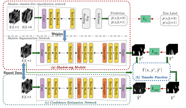
Figure 2: Training framework of the proposed method. (a) The shadow-seg module containing a shadow/shadow-free classification network and a shadow segmentation network. (b) The transfer function that expands a binary mask to a reference confidence map. (c) The confidence estimation network which establishes direct mapping between input images and confidence maps.

Shadow-seg Module

We propose a shadow-seg module to extract generalized shadow features for a large range of shadow types in fetal US images under limited weak manual annotations. Since shadow regions have different shapes, various intensity distributions and uncertain edges, the pixel-wise annotation of shadow regions is time consuming and relies heavily on annotator’s experience (e.g. various annotations in Fig. 1(b)). This generally results in manual annotations of limited quantity and quality. Compared with pixel-wise shadow annotations, global image-level labels (“has shadow” and “shadow-free” in our case) are easier to obtain, and shadow images with global image-level labels can contain a larger variety of shadow types. Therefore, we use a shadow-seg module that combines unreliable pixel-wise annotations and global image-level labels as weak annotations.The proposed shadow-seg module contains two tasks, (1) shadow/shadow-free classification using image-level labels, and (2) shadow segmentation that uses few coarse pixel-wise manual annotations ($10\%$ of the global image-level labels). Shadow features can be extracted during simple shadow/shadow-free classification and subsequently optimized for the more challenging shadow segmentation task. In our case, shadow features extracted by the classification network cover various shadow types in a range of anatomical structures. These shadow features become suitable for the shadow segmentation after being optimized by a shadow segmentation network.

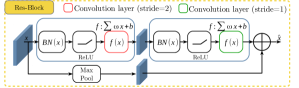
Figure 3: The architecture of the residual-block. $BN(x)$ refers to a batch normalization layer and $f(x)$ is a convolutional layer.

Network Architecture

We build two sub-networks from residual-blocks [14] as shown in Fig. 3. Residual-blocks can reduce the training error when using deeper networks and support better network optimization [14]. They have been widely used for various image processing algorithms [38, 13, 36]. The first and initially trained network is a shadow/shadow-free classification network that learns to distinguish images containing shadows from shadow-free images, and thus learns the defining features of acoustic shadow. This classification network consists of a feature encoder followed by a global average pooling layer. The feature encoder uses six residual-blocks (Fig. 3) to extract shadow features that define shadow-containing images in the classifier. We refer to $l=1$ as the label of the shadow-containing class and $l=0$ as the label of the shadow-free class. Image set $X^{C}=\{x_{1}^{C},x_{2}^{C},...,x_{K}^{C}\}$ and their corresponding labels $L=\{l_{1},l_{2},...,l_{K}\}\text{ s.t.}l_{i}\in\{0,1\}$ are used to train the feature encoder as well as the global average pooling layer. We use softmax cross-entropy loss as the cost function $L_{C}$ between the predicted labels and the true labels.

Representative shadow features extracted by the feature encoder of the shadow/shadow-free classification network are then optimized by the shadow segmentation network with a limited number of densely segmented US images. The feature encoder of the segmentation network has the same architecture as the classification network. The weights of the feature encoder in the segmentation network are initialized by that of the classification network and are further fine-tuned for the segmentation task. Therefore, the extracted shadow features are suitable for the segmentation in addition to classification. The decoder of the segmentation network is symmetrical to the feature encoder. Feature layers from the feature encoder are concatenated to the corresponding layers in the decoder by skip connections. Here, we denote the image set used to train the shadow segmentation with $X^{S}=\{x_{1}^{S},x_{2}^{S},...,x_{M}^{S}\}$ and the corresponding pixel-wise manual segmentation with $Y^{S}=\{y_{1}^{S},y_{2}^{S},...,y_{M}^{S}\}$. The shadow segmentation provides a pixel-wise binary prediction $\hat{Y}^{S}=\{\hat{y}_{1}^{S},\hat{y}_{2}^{S},...,\hat{y}_{M}^{S}\}$ for shadow regions and the cost function $L_{seg}$ is the softmax cross-entropy between $\hat{Y}^{S}$ and $Y^{S}$.

Transfer Function

Binary masks lack information about inherent uncertainties at the boundaries of shadow regions. Therefore, we use a transfer function to extend the binary segmentation prediction to a confidence map, which is more appropriate to describe shadow regions. The main task of the transfer function is to learn the intensity distribution of shadow regions so as to estimate confidence of pixels in false positive (FP) regions of the predicted binary shadow segmentation. This transfer function is built and only used during training to provide reference confidence maps for the confidence estimation network.

When comparing the manual segmentation $y^{S}$ and the predicted segmentation $\hat{y}^{S}$ of shadow regions in image $x$, we define the true positive (TP) regions $x_{TP}$ as shadow regions with the full confidence, $C_{x_{ij}}=1,x_{ij}\in x_{TP}$. Here, $C_{x_{ij}}$ refers to the confidence of pixel $x_{ij}$ being shadow.

For each pixel $x_{ij}$ in the FP regions ($x_{FP}$), the confidence of belonging to a shadow region is computed by a transfer function $T(x_{ij}\mid x_{ij}\in x_{FP})$ based on the intensity of the pixel ($I_{x_{ij}}$) and the mean intensity of $x_{TP}$ ($I_{mean}$). $I_{mean}$ is defined in Eq. 1. With weak signals in the shadow regions, the average intensity of shadow pixels is lower than the maximum intensity ($I_{max}=max(x)$) but not lower than the minimum intensity ($I_{min}=min(x)$), that is $I_{mean}\in[I_{min},I_{max})$.

$$I_{mean}=\begin{cases}mean(y^{S}\cap\hat{y}^{S})&y^{S}\cap\hat{y}^{S}\neq\emptyset,\\ mean(y^{S})&y^{S}\cap\hat{y}^{S}=\emptyset,\end{cases}$$ (1)

The transfer function $T(\cdot)$ computing $C_{x_{ij}}$ for pixels in $x_{FP}$ is defined according to the range of $I_{mean}$. For $I_{mean}\in(I_{min},I_{max})$, $T(\cdot)$ is shown in Eq. 2. For $I_{mean}=I_{min}$, $T(\cdot)$ is shown in Eq. 3.

$$T(x_{ij}\mid x_{ij}\in x_{FP})=\begin{cases}\frac{I_{x_{ij}}-I_{min}}{I_{mean}-I_{min}},&I_{min}\leq I_{x_{ij}}<I_{mean},\\ \frac{I_{max}-I_{x_{ij}}}{I_{max}-I_{mean}},&I_{mean}<I_{x_{ij}}\leq I_{max},\\ 1,&I_{x_{ij}}=I_{mean},\end{cases}$$ (2)

$$T(x_{ij}\mid x_{ij}\in x_{FP})=\begin{cases}\frac{I_{x_{ij}}-I_{mean}}{I_{max}-I_{mean}},&I_{mean}<I_{x_{ij}},\\ 1,&I_{x_{ij}}=I_{mean},\end{cases}$$ (3)

After using the transfer function, the binary map of the predicted segmentation $y^{S}$ is extended to a confidence map $y^{C}$. $y^{C}$ acts as a reference (”ground truth”) for the training of the next confidence estimation network.

Confidence Estimation Network

After obtaining reference confidence maps from the predicted binary segmentation, a confidence estimation network is trained to map an image with shadows ($x$) to the corresponding reference confidence map ($y^{C}$). This confidence estimation network can be independently used to directly predict a dense shadow confidence map for an input image during inference.

The confidence estimation network consists of a down-sampling encoder, a symmetric up-sampling decoder, and skip connections between feature layers from the encoder and the decoder at different resolution levels. Both the encoder and the decoder are composed of six residual-blocks. The cost function of the confidence estimation network is defined as the mean squared error between the predicted confidence map $\hat{Y}^{C}$ and the reference confidence map $Y^{C}$ ($\mathcal{L}_{conf}=\lVert\hat{Y}^{C}-Y^{C}\rVert_{2}$).

Attention Gates

Attention gates are believed to generally highlight relevant features according to image context and thus improve network performance for medical image analysis [25]. We integrate attention gates [30] into our approach to explore if attention mechanisms can further improve the confidence estimation of shadow regions in 2D ultrasound. In our case, we connect the self-attention gating modules proposed in [25] to the feature maps before the last two down-sampling operations in the encoders of all three networks. For the shadow/shadow-free classification network, the global average pooling layer is modified when adding this self-attention gating module. In detail, as shown in Fig. 4, the global average pooling layers are operated separately on the two attention-gated feature maps as well as the original last feature map to obtain three average feature maps. These three average feature maps are then concatenated, followed by a fully connected layer to compute the final classification prediction.

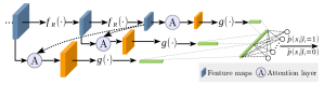
Figure 4: The architecture of the shadow/shadow-free classification network with attention mechanism. $f_{R}(\cdot)$ refers to residual-blocks. $g(\cdot)$ refers to a global average pooling layer.

III Implementation

All the residual-blocks used in the proposed method are implemented as proposed in [26], which provides a convenient interface to realize residual-blocks.

We optimize the different modules separately and consecutively in three steps. First we train $\sim 70$ epochs for the parameters of the shadow/shadow-free classification network, and then $\sim 700$ epochs for the pixel-wise shadow segmentation network. After obtaining a well-trained shadow segmentation network, we train the confidence estimation network for another 700 epochs.

For all networks, we use Stochastic Gradient Descent (SGD) with momentum optimizer to update the parameters since SGD has better generalization capability than adaptive optimizer [35]. The parameters of the optimizer are $momentum=0.9$, with a learning rate of $10^{-3}$. We apply L2 regularization to all weights during training to help prevent network over-fitting. The scale of the regularizer is set as $10^{-5}$. The training batch size is 25 and our networks are trained on a Nvidia Titan X GPU with 12 GB of memory.

IV Evaluation

The proposed method is trained and evaluated using two data sets, (1) a multi-class data set consisting of 13 classes of 2D US fetal anatomy with global image-level label (“has shadow” or “shadow-free”) and including 48 non-brain images with manual shadow segmentations, and (2) a single-class data set containing 2D US fetal brain with coarse pixel-wise manual shadow segmentations. To reduce the variance in parameter estimation during training, we split relatively bigger training data sets. In the multi-class data set, we use $88\%$ of the data for training, $11\%$ for validation and the 48 non-brain images for testing, while in the single-class data set we use $78\%$ of the data for training, $8\%$ for validation and $14\%$ for testing.

To verify the effectiveness of the proposed method and the importance of the shadow/shadow-free classification network in the shadow-seg module, we compare the variants of our method to a baseline which only contains a shadow segmentation network and a confidence estimation network.

We use standard measurements such as Dice coefficient (DICE) [11], recall, precision and Mean Squared Error (MSE) for shadow segmentation evaluation, and use the Interclass Correlation (ICC) [31] as well as soft DICE [2] for confidence estimation evaluation. In order to verify the performance of our method, we also compute quantitative measurements between the chosen manual annotation (weak ground truth) and another manual annotation from a different annotator to show the human performance for the shadow detection task. Lastly, we show the practical benefits of shadow confidence maps for different applications such as a standard plane classification task, an image fusion task from multiple views and a segmentation task for automatic biometric measurements.

Multi-class Data Set

This data set consists of $\sim 8.5k$ 2D fetal US images sampled from 13 different anatomical standard plane locations as defined in the UK FASP handbook [23]. These images have been sampled from 2694 2D ultrasound examinations from volunteers with gestational ages between $18-22$ weeks (iFIND Project ). Eight different ultrasound systems of identical make and model (GE Voluson E8) were used for the acquisitions. Various image settings based on different sonographers’ personal preference for scanning are included in this data set. The images have been classified by expert observers as containing strong shadow, being shadow-free, or being corrupted, e.g. poor tissue contact caused by lacking acoustic impedance gel. Corrupted images ($<3\%$) have been excluded as discussed in Section VI with Fig. 10.

Single-class Data Set

This data set comprises 643 fetal brain images and has no overlap with the multi-class data set. Shadow regions in this data set have been coarsely segmented by two bio-engineering students using trapezoid-shaped segmentation masks for individual shadow regions.

Training Data

3448 shadow images and 3842 clear images have been randomly selected from the multi-class data set to train the shadow/shadow-free classification network. 500 fetal brain images have been randomly chosen from the single-class data set to train the shadow segmentation network, and the confidence estimation network. These 500 fetal images have been flipped as data augmentation during training.

Validation and Test Data

The remaining 491 shadow images and 502 clear images in the multi-class data set are used for testing and validation. Here, a subset ($M_{test}$) comprising 48 randomly selected images from the 491 shadow images is used for testing. These 48 images contain various fetal anatomies (except fetal brain), such as abdominal, kidney, cardiac and etc. Shadow regions in these images have been manually segmented to provide ground truth. The remaining 443 shadow images and 502 clear images are used for the validation of the shadow/shadow-free classification. Similarly, the remaining 143 fetal brain images of the single-class data set are split into two subsets, where $S_{val}$ contains 50 images for validation of the shadow segmentation, binary-to-confidence transformation and the confidence estimation, and $S_{test}$ with 93 images for testing. For all images from the single-class data set, we randomly choose one group of annotations from two different existing groups of annotations as ground truth for training, validation and testing.

IV-A Baseline

The baseline method is used to demonstrate that the shadow-seg module is of importance for capturing generalized shadow features and obtaining accurate confidence estimation of shadow regions. It comprises a shadow segmentation network and a confidence estimation network, which have the same architectures as shown in Fig. 2. We firstly train the shadow segmentation network in the baseline method using the 500 fetal brain images from the single-class data set. After applying the transfer function on the binary segmentation prediction, we train the confidence estimation network for a direct mapping between shadow images and reference confidence maps.

IV-B Evaluation Metrics

In this section, we define the aforementioned statistical metrics and the computation of the inter-observer variability between two pixel-wise manual annotations of shadow regions.

DICE, Recall, Precision and MSE

We refer to the binary prediction of shadow segmentation as $P$ and the binary manual segmentation as $G$. $\text{DICE}=2|P\cap G|/(|P|+|G|)$, $\text{Recall}=|P\cap G|/|G|$, $\text{Precision}=|P\cap G|/|P|$ and $\text{MSE}=|P-G|$.

ICC

We use $ICC$ as proposed by [31] (Eq. 4) to measure the agreement between two annotations. Each pixel in an image is regarded as a target. $R_{MS}$, $C_{MS}$ and ${M}_{MS}$ are respectively mean squared value of rows, columns and interaction. $N$ is the number of targets.

$$ICC=\frac{R_{MS}-{M}_{MS}}{R_{MS}+{M}_{MS}+2\times(C_{MS}-{M}_{MS})/N}.$$ (4)

Soft DICE

Soft DICE can be used to tackle probability maps. We use real-value in the DICE definition to compute soft DICE between the predicted shadow confidence maps $\hat{Y}^{C}$ and reference confidence maps $Y^{C}$.

Human Performance

We consider another binary segmentation of shadow regions from a different annotator as $Y^{S}_{new}$. The computed metrics between $Y^{S}_{new}$ and the chosen manual segmentation $Y^{S}$ reflects the human inter-observer variability.

IV-C Shadow Segmentation Analysis

We compare the segmentation performance of the state-of-the-art ([16] and [22]), the proposed methods and the human performance. This comparison is used to examine the importance of the shadow-seg module for the shadow segmentation, and further, for the confidence estimation of shadow regions.

TABLE I: Shadow segmentation performance ($\mu\pm\sigma$) of different methods on test data $S_{test}$. RW and $\text{RW}^{\ast}$ are Random Walk algorithm [16] with different set of parameters. Pilot [22] is our previous work. Baseline, the proposed method (abbreviated as “Proposed”) and the proposed method with attention gates (abbreviated as “Proposed$+$AG” in the rest of the paper) are our proposed methods. $\text{Anno}^{\ast}$ refers to the human inter-observer variability, thus expected human performance on the shadow segmentation task. Best results are shown in bold.

Methods		DICE	Recall	Precision	MSE
RW [16]	$\mu$	0.2096	0.6535	0.1288	194.8618
	($\sigma$)	(0.099)	(0.2047)	(0.0675)	(7.6734)
$\text{RW}^{\ast}$ [16]	$\mu$	0.231	0.6921	0.1432	189.0828
	($\sigma$)	(0.1123)	(0.2196)	(0.0771)	(8.3484)
Pilot [22]	$\mu$	0.3227	0.4275	0.2863	110.2959
	($\sigma$)	(0.1398)	(0.201)	(0.1352)	(14.837)
Baseline	$\mu$	0.6933	0.6884	0.7246	60.3680
	($\sigma$)	(0.212)	(0.2255)	(0.2326)	(12.2885)
Proposed	$\mu$	0.7167	0.7217	0.7382	58.6974
	($\sigma$)	(0.1988)	(0.2131)	(0.2255)	(11.867)
Proposed$+$AG	$\mu$	0.7027	0.7199	0.7132	61.241
	($\sigma$)	(0.2014)	(0.2169)	(0.2247)	(12.6317)
$\text{Anno}^{\ast}$	$\mu$	0.5443	0.6126	0.567	65.7286
	($\sigma$)	(0.2635)	(0.3196)	(0.3124)	(23.0339)

Table I shows DICE, recall, precision and MSE of different methods on $S_{test}$. RW and $\text{RW}^{\ast}$ are results of [16] with various parameters. For fair comparison, we run 24 tests on both test sets using the RW algorithm with different parameter combinations ($\alpha\in\{1,2,6\}$; $\beta\in\{90,120\}$; $\gamma\in\{0.05,0.1,0.2,0.3\}$). With a negative relationship between the likelihood of shadows and the confidence in [16] and to consistently compare all methods, we use $1-S$ instead $S$ to display the results of RW and $\text{RW}^{\ast}$ in all comparison experiments. Here $S$ is a confidence map obtained by [16]. To generate shadow segmentation, we threshold the obtained confidence maps by $T\in\{0.25,0.3\}$ so that pixels with confidence higher than $T$ are shadows. We chose the parameters and the threshold which achieve the highest average DICE on all samples in both test sets. The chosen RW parameters and the threshold are $\alpha=1$; $\beta=90$; $\gamma=0.3$; $T=0.3$. We also applied the parameters and the threshold in [16] ($\alpha=2$; $\beta=90$; $\gamma=0.05$; $T=0.25$) in our experiments, which is denoted as $\text{RW}^{\ast}$. Note that we use the public Matlab code  of [16] to test RW and $\text{RW}^{\ast}$.

As shown in Table I, the baseline, the proposed method and the proposed$+$AG greatly outperform the state-of-the-art. Among all methods, the proposed method achieves highest DICE. Recall and precision of the proposed method are respectively $3.33\%$ and $1.16\%$ higher than that of the baseline while MSE of the proposed method is $1.67$ lower than that of the baseline. After adding attention gates to the proposed method (the proposed$+$AG), the shadow segmentation performance is nearly the same to the proposed method without attention gates, but better than the baseline. Additionally, the relatively low scores of $\text{Anno}^{\ast}$ indicate high inter-observer variability and how ambiguous human annotation can be for this task. A mean DICE of $0.7167$ shows that the proposed method performs better and more consistently than human annotation.

TABLE II: Comparison of shadow segmentation performance ($\mu\pm\sigma$) of different methods on test data $M_{test}$. Best results are shown in bold.

Methods		DICE	Recall	Precision	MSE
RW [16]	$\mu$	0.1795	0.8456	0.1038	193.2229
	($\sigma$)	(0.0855)	(0.1241)	(0.0592)	(7.866)
$\text{RW}^{\ast}$ [16]	$\mu$	0.1766	0.8038	0.1025	190.5627
	($\sigma$)	(0.0871)	(0.1528)	(0.0602)	(7.5643)
Pilot [22]	$\mu$	0.467	0.728	0.371	86.9005
	($\sigma$)	(0.1079)	(0.137)	(0.1308)	(17.0491)
Baseline	$\mu$	0.4765	0.5026	0.5108	68.5054
	($\sigma$)	(0.1798)	(0.2233)	(0.1712)	(18.3773)
Proposed	$\mu$	0.5463	0.5968	0.565	64.6912
	($\sigma$)	(0.155)	(0.2335)	(0.1357)	(17.2147)
Proposed$+$AG	$\mu$	0.5302	0.5741	0.5454	66.4474
	($\sigma$)	(0.1544)	(0.2035)	(0.1562)	(17.6628)

• The symbols of the methods are the same to Table I.

We further conduct the same experiments on another non-brain test data set $M_{test}$ to verify the feature generalization ability of the shadow-seg module. Results are shown in Table II. Similarly, the proposed weakly supervised methods and the baseline outperform all state-of-the-art methods.

To statistically evaluate the difference among various methods, we use the paired sample t-test on two test data sets $S_{test}$ and $M_{test}$. Here, we compare the evaluation metrics (Dice, Recall, Precision and MSE) of the proposed method and the Pilot [22] because the Pilot [22] outperforms other state-of-the-art in Table I and Table II. We also compare the evaluation metrics of the proposed method and the baseline. The obtained corresponding p-values are shown in Table III, using $0.01$ as the threshold for statistical significance, Table III shows that the proposed method greatly improves the shadow segmentation performance compared with the Pilot [22] and the baseline.

TABLE III: The p-value of the Proposed method vs. Pilot [22] and of the Proposed method vs. Baseline. Statistically significant results ($p<0.01$) are shown in bold.

	$S_{test}$
	DICE	Recall	Precision	MSE
Pilot [22]	0.0001	0.0001	0.0001	0.0001
Baseline	0.0015	0.001	0.0694	0.012
	$M_{test}$
	DICE	Recall	Precision	MSE
Pilot [22]	0.0032	$\text{0.0013}^{\dagger}$	0.0001	0.0001
Baseline	0.0001	0.0001	0.0037	0.0014

• refers to the proposed method performs worse and otherwise the proposed method is better.

IV-D Shadow Confidence Estimation

In this part, we evaluate the performance of the confidence estimation by comparing the shadow confidence maps of different methods.

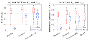
Figure 5: Results of shadow confidence estimation. (a) Soft DICE of the baseline, the proposed method and the proposed method with attention gates (proposed$+$AG) on $S_{test}$ and $M_{test}$. (b) Interclass correlation (ICC) of the baseline, the proposed method and the proposed$+$AG on $S_{test}$ and $M_{test}$. Additionally, ICC of the human performance is shown as $\text{Anno}^{\ast}$ for $S_{test}$.

Fig. 5 (a) shows the soft DICE evaluation on $S_{test}$ and $M_{test}$. The proposed method and the proposed$+$AG method achieve higher soft DICE on both test sets than the baseline, and are more robust than the baseline on $M_{test}$. The baseline fails in this experiment on $M_{test}$ because it is unable to obtain accurate shadow segmentation in the previous step (shown in Table II). With less accurate shadow segmentation, the shadow confidence estimation can hardly establish a valid mapping between input images and reference confidence maps. This demonstrates that the shadow-seg module is beneficial for shadow segmentation and confidence estimation.

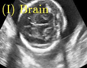
(a)

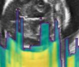
(b)

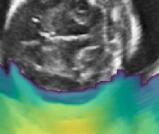
(c)

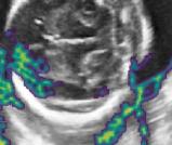
(d)

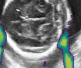
(e)

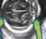
(f)

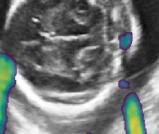
(g)

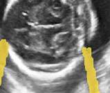
(h)

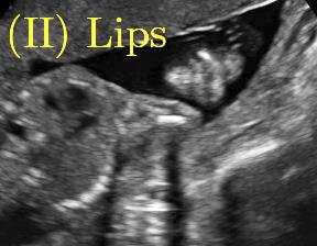
(i)

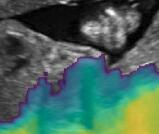
(j)

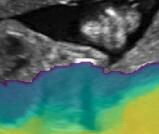
(k)

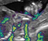
(l)

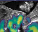
(m)

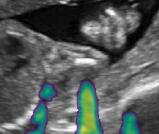
(n)

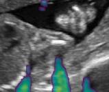
(o)

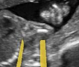
(p)

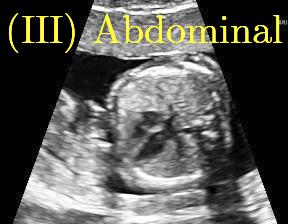
(q)

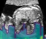
(r)

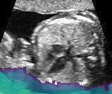
(s)

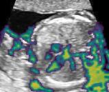
(t)

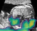
(u)

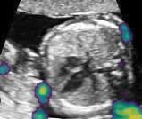
(v)

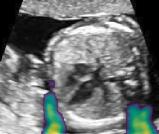
(w)

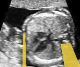
(x)

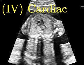
(a) Image

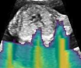
(b) RW [16]

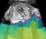
(c) $\text{RW}^{\ast}$ [16]

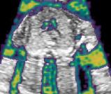
(d) Pilot [22]

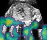
(e) Baseline

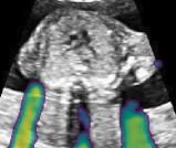
(f) Proposed

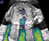
(g) Proposed+AG

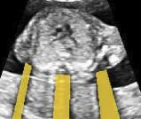
(h) Weak GT

Figure 6: Confidence estimation of shadow regions using the state-of-the-art methods and our methods. Rows I-IV show four examples: Brain (top), Lip (second), Abdominal (third) and Cardiac (bottom). Column (a) is the original US image. Columns (b-d) are shadow confidence maps from the RW algorithm [16] and our previous work [22]. Columns (e-g) show the shadow confidence maps of the baseline, the proposed method and the Proposed$+$AG method. Column (h) is the binary map of the manual shadow segmentation. The color bar on the top of this figure shows that the more yellow/brighter (closer to 1), the higher the confidence of being shadow regions.

We additionally evaluate the reliability of the shadow confidence estimation by measuring the agreement between the decision of each method and the manual segmentation. Regarding the baseline, the proposed and the proposed$+$AG as different judges and the manual segmentation of shadow regions as a contrasting judge, we use the ICC to measure the agreement between each different judge and the contrasting judge. Fig. 5 (b) shows the ICC evaluation on two test data sets, which indicate that the proposed method and the proposed$+$AG are more consistent on estimating shadow confidence maps compared with the baseline. When considering another manual segmentation of shadow regions as an extra judge, we can evaluate the agreement of human annotations. Fig. 5 (b) shows that the ICC of two human annotations (shown as Anno) is normally $0.51$. The proposed method with an ICC of $0.66$ is more consistent than annotations from two human annotators.

Fig. 6 compares the shadow confidence maps of the state-of-the-art methods and the proposed methods. RW and $\text{RW}^{\ast}$ have the same parameters as used for Table I. The shadow confidence maps of the baseline, the proposed method and the proposed$+$AG method are generated directly from input shadow images by confidence estimation networks. Overall, the proposed method and the proposed$+$AG method achieve more visually reasonable shadow confidence estimation than the baseline and the state-of-the-art on different anatomical structures shown in Fig. 6. The proposed method and the proposed$+$AG method are able to highlight multiple shadow regions while the RW algorithm shows limitations for most cases, especially for disjoint shadow regions.

Row I in Fig. 6 shows a fetal brain image from $S_{test}$. The confidence estimation of shadow regions from the baseline, the proposed method and the proposed$+$AG method are similarly accurate since we use fetal brain images to train the confidence estimation networks in these three methods. These outperform [16] and [22]. Rows (II-IV) in Fig. 6 show shadow confidence maps of non-brain anatomy from $M_{test}$, including lips, abdominal and cardiac. The baseline failed on unseen data during inference. However, the proposed methods are able to generate accurate shadow confidence maps because of the generalized shadow features obtained by the shadow-seg module. Furthermore, the “Lips” example shows that our method is capable of detecting weaker shadow regions that have not been annotated in manual segmentation. This indicates that the confidence estimation network has learned general properties of shadow regions.

IV-E Transfer Function Performance

We show two illustrative examples in Fig. 7 to demonstrate the performance of the transfer function. Fig. 7 (c) and (d) show that the transfer function computes the confidence of each pixel in the false positive areas of the predicted segmentation, so that to extend a binary segmentation to a reference confidence map.

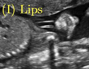
(a)

(b)

(c)

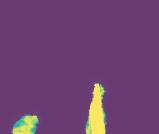
(d)

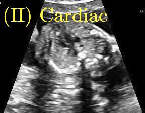
(a) Image

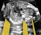
(b) Weak GT

(c) $\hat{Y}^{S}$

(d) $Y^{C}$

Figure 7: Two examples showing the performance of the transfer function. (a) is the input image and (b) is the binary manual segmentation. (c) is the predicted segmentation before applying the transfer function while (d) is the corresponding reference confidence map after the transfer function.

IV-F Runtime

The RW algorithm [16] is implemented in Matlab (CPU Xeon E5-2643) while the previous work [22] and the proposed methods use Tensorflow and run on a Nvidia Titan X GPU. For the RW algorithm [16] and the previous work [22], the inference time are $0.4758s$ and $11.35s$ respectively. Since the baseline, the proposed method and the proposed$+$AG method have the same confidence estimation networks, they have the same inference time, which is $0.0353s$. A system-independent evaluation can be performed by estimating the required Giga-floating point operations (GFlops, fused multiply-adds) during inference. Our method requires $\sim 2.5-3$ GFlops (estimated from conv-layers including ReLU activation, Appendix -I, supplementary materials are available in the supplementary files /multimedia tab.) while the RW algorithm [16] requires $\sim 4-4.5$ GFlops (according to the built-in Matlab profiler) and the previous work [22] requires $\sim 19$ GFlops (estimated from conv-layers including ReLU activation, Appendix -I).

V Applications

To verify the practical benefits of our method, we integrate the shadow confidence maps into different applications such as 2D US standard plane classification, multi-view image fusion and automated biometric measurements.

V-A Ultrasound Standard Plane Classification

Classifying 2D fetal standard planes is of great importance for early detection of abnormalities during mid-pregnancy [29]. However, distinguishing different standard planes is a challenging task and requires intense operator training and experience. Baumgartner et al. [3] have proposed a deep learning method for the detection of various fetal standard planes. We extend [3] and utilize shadow confidence maps to provide extra information for standard plane classification.

The data is the same as used in [3], which is a set of $2694$ 2D ultrasound examinations between 18-22 weeks of gestation (iFIND Project 1). We select nine classes of standard planes including Three Vessel View (3VV), Four Chamber View (4CH), Abdominal, Brain View at the level of the cerebellum (Brain (cb.)), Brain view at posterior horn of the ventricle (Brain (tv.)), Femur, Lips, Left Ventricular Outflow Tract (LVOT) and Right Ventricular Outflow Tract (RVOT). The data set is split into training ($16089$), validation ($450$), and testing ($4368$) images, similar to [3] (see section -E for individual class split numbers). We use image whitening (subtracting the mean intensity and divide by the variance) on each image to preprocess the whole data set.

Four networks based on SonoNet-32 [3] are trained and tested in order to verify the utility of shadow confidence maps. The first network is trained with the standard plane images from the training data. The next three networks are separately trained with standard plane images and their corresponding shadow confidence maps obtained by the baseline, the proposed method and the proposed$+$AG method. Thus, the training data in the first network has one channel while the remaining networks have two input channels. We train these networks for $75$ epochs with a learning rate of $0.001$.

Table IV shows the standard plane classification performance of the four networks. Networks with shadow confidence maps achieve higher classification accuracy on almost all classes (except Abdominal, LVOT and RVOT), as well as on average classification accuracy. $CM_{PAG}$ achieves highest classification accuracies for five classes (3VV, 4CH, Brain(Cb.), Brain(Tv.) and Femur). Of particular note, the accuracies of the 3VV and 4CH classes increase over the baseline by $11.75\%$ and $5.5\%$ respectively. Five other classes (Abdominal, Brain(Cb.), Brain(Tv.), Femur and Lips) achieve near $100\%$ accuracy in both the baseline and $CM_{PAG}$, while LVOT and RVOT classes see modest decreases in $CM_{PAG}$ compared with the baseline, $2.1\%$ and $1.0\%$ respectively. Therefore, when compared $CM_{PAG}$ with the baseline, the increase in average classification accuracy across all classes ($97.37\%$ to $98.74\%$) is primarily driven by the large improvements in 3VV and 4CH. These results indicate that shadow confidence maps are able to provide extra information and improve the performance of another automatic medical image analysis algorithm.

TABLE IV: Classification accuracy ($\%$) with vs. without shadow confidence maps. w/o $CM$ is the network without shadow confidence maps while ${CM}_{B}$, ${CM}_{P}$ , ${CM}_{PAG}$ are networks with shadow confidence maps from the baseline, the proposed method and the proposed+AG method. Best results are shown in bold.

Class	w/o $CM$	${CM}_{B}$	${CM}_{P}$	${CM}_{PAG}$
3VV	80.87	89.93	88.93	92.62
4CH	94.50	100.00	98.38	100.00
Abdominal	100.00	99.82	99.28	99.82
Brain(Cb.)	100.00	99.84	100.00	100.00
Brain(Tv.)	99.11	99.78	99.78	99.89
Femur	99.04	99.81	99.81	99.81
Lips	98.29	99.81	100.00	99.81
LVOT	97.90	93.69	94.29	95.80
RVOT	95.95	93.24	92.57	94.93
Avg.	97.37	98.24	98.03	98.74

We additionally explore the importance of estimating confidence maps over binary segmentation of shadow regions. We compare the classification accuracy between using shadow confidence maps and directly using binary shadow segmentations generated from different methods. Fig.8 shows that for classes with high classification accuracy such as Abdominal, Brain(Cb.), Brain(Tv.), Femur and Lips, integrating shadow confidence maps into the classification task yields minor improvement. However, for classes with relatively low classification accuracy such as 3VV and LVOT, classification with shadow confidence maps achieves higher accuracy than classification with only binary shadow segmentations.

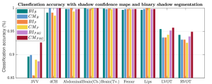
Figure 8: Comparison of classification accuracy between using shadow confidence maps and using shadow segmentation. ${BI}_{B}$, ${BI}_{P}$ and ${BI}_{PAG}$ are networks with binary shadow segmentation from the baseline, the proposed method and the proposed$+$AG method. ${CM}_{B}$, ${CM}_{P}$ and ${CM}_{PAG}$ are the same networks as in Tabel IV.

V-B Multi-view Image Fusion

Routine US screening is usually performed using a single 2D probe. However, the position of the probe and resulting tomographic view through the anatomy has great impact on diagnosis. Zimmer et al. [39] proposed a multi-view image reconstruction method, which compounds different images of the same anatomical structure acquired from different view directions. They use a Gaussian weighting strategy to blend intensity information from different views. Here, we combine predicted shadow confidence maps from these multi-view images as additional image fusion weights to investigate if these confidence maps can further improve image quality.

The proposed method generally outperforms the baseline and the proposed$+$AG method, thus we only integrate the shadow confidence maps generated by the proposed method (${CM}_{P}$) into the weighting strategy in [39]. In detail, the probability value of each pixel in a shadow confidence map is multiplied to the original weight of the same pixel computed in [39]. The generated new weights are normalized as described in [39] and then are used for image fusion. The data set in this experiment is same as used for [39].

Fig. 9 qualitatively shows that shadow confidence maps are able to improve the performance of US image fusion algorithms with different weighting strategies. Fig. 9 also shows the difference between adding two different types of confidence maps. These two types of confidence maps are generated by the confidence estimation network which are separately trained by either MSE or Sigmoid loss. Fig. 9 (a) to (d) illustrate image fusion results for the same case using different combinations of weighting strategies and loss functions. The difference maps indicate that shadow confidence maps are capable of improving image fusion performance. Fig. 9 (e) to (h) show image fusion results on four different cases. We randomly select two positively affected cases (Fig. 9 (e) and (f)) to show visual improvement. We additionally show two randomly selected examples (Fig. 9 (g) and (h)) that don’t show perceptually significant improvements after adding shadow confidence maps. Quantitative evaluation for image fusion is not possible because of lacking a ground truth for US compounding tasks.

(a) Gaussian, MSE

(b) Int. & Gaussian, MSE

(c) Gaussian, Sigmoid

(d) Int. & Gaussian, Sigmoid

(e) Gaussian, MSE, $+$

(f) Int. & Gaussian, Sigmoid, $+$

(g) Gaussian, Sigmoid, $-$

(h) Int. & Gaussian, Sigmoid, $-$

Figure 9: Results of image fusion based on different weighting strategies and loss functions (Gaussian weighting vs. Intensity-and-Gaussian weighting (Int. & Gaussian), MSE loss vs. Sigmoid loss). Note that the MSE loss and the Sigmoid loss are used for training of the confidence estimation network, which generates the shadow confidence maps. (a-d) are the image fusion results of the same case. (a,c) are the image fusion of Gaussian weighting with MSE loss and Sigmoid loss respectively and (b,d) are the results of Intensity-and-Gaussian weighting with MSE loss and Sigmoid loss respectively. (e-h) show the image fusion results on four different cases. (e,f) are examples for visually improved cases ($+$) showing notable positive differences of image fusion before and after adding ${CM}_{P}$ confirmed by our sonographers while (g,h) are cases with less change ($-$). For each sub-figure (e.g. (a)), in the first column, the top row is the result without integrating a shadow confidence map ${CM}_{P}$ and the bottom row is the result with integrated ${CM}_{P}$. The second column shows the corresponding enlarged framed areas of the images. The third column is the difference map of corresponding framed areas. The color bar on the top shows that the more yellow/brighter, the higher the difference between the two framed areas.

V-C Automated Biometric Measurements

We integrate our shadow confidence maps into an automatic biometric measurement approach [32], and show the biometric measurement performance (measured by DICE) before and after adding shadow confidence maps.

Similar to the ultrasound standard plane classification, shadow confidence maps are integrated into a biometric estimation model described in [32] as an extral channel. Specifically, we train and test four fully convolutional networks with the same hyper-parameters as detailed in  [32], and use the same ellipse fitting algorithm described therein. The first network is trained only on the image data used in [32]. The other three networks are trained with an additional input channel for shadow confidence maps that are separately generated by the baseline, the proposed, and the proposed$+$AG method.

We show three examples that are affected by shadows, and show their biometric measurement results in Table V. From this experiment, we find that biometric measurement performance is boosted by up to $7\%$ for problematic failure cases after adding shadow confidence maps. The average performance on the entire test data set stays almost the same since only a small proportion of the test images are affected by strong shadows, mainly because of the image acquisition by highly skilled sonographers.

TABLE V: Biometric measurement performance (DICE) with vs. without shadow confidence maps.

	w/o $CM$	${CM}_{B}$	${CM}_{P}$	${CM}_{PAG}$
$\#1$	0.947	0.940	0.988	0.969
$\#2$	0.956	0.958	0.974	0.968
$\#3$	0.880	0.915	0.923	0.955
Avg.	0.966	0.964	0.965	0.964

• The symbols of the methods are the same to Table IV.

VI Discussion

In this paper, we propose a weakly supervised method to tackle the ill-defined problem of shadow detection in US. A naïve alternative to our method would be to train a fully supervised shadow segmentation network using pixel-wise annotation of shadow regions. However, pixel-wise annotation is infeasible because (a) accurately annotating a large number of images requires a vast amount of labour and time and has scanner dependencies (b) binary annotations of shadow regions would lead to high inter-observer variability as shadow features are poorly defined, and (c) real-valued annotations of shadow regions are affected by subjectivity of annotators.

The performance of shadow region confidence estimation on different anatomical structures can be improved after integrating attention mechanisms. For example, the soft DICE is increased on $S_{test}$. This also results in improved ultrasound classification (Table IV). However, the quantitative results show that attention mechanisms are not essential. Networks with attention mechanisms are sometimes outperformed by networks without attention mechanisms. This may be caused by the way we integrate the attention mechanism. Since we add attention gates to encoders of all networks, the shadow features are emphasized for the shadow/shadow-free classification, which increases the difficulty of generalizing shadow features from classification to shadow segmentation.

We use MSE as the loss function of the confidence estimation network, but this loss can also be measured by other functions. Practically this choice has no effect on our quantitative results. However, in the image fusion task, we observe qualitative differences, which we show in Fig. 9 for Sigmoid cross-entropy loss.

In the standard plane classification task, we use only a subset of target standard planes compared to [3] because (1) we aim at verifying the usefulness of our method rather than improving performance of [3], (2) it is desirable to keep inter-class balance to avoid side-effects from under-represented classes, and (3) we chose standard planes for which [3] did not show optimal classification performance.

$T(\cdot)$, as defined in Eq. 2 or Eq. 3 is one example how prior knowledge can be integrated into the training process. If $T(\cdot)$ is chosen to be a continuous non-trainable function, e.g. quadratic or Gaussian, further weight relaxation can be introduced for joint refinement of both, the shadow-seg module in Fig. 2a and the confidence estimation in Fig. 2c. However, since probabilistic ground truth does not exist for our applications, evaluation would become purely subjective, thus we decide to use direct but discontinuous integration of shadow-intensity assumptions for $T(\cdot)$.

Task-specific deep networks, e.g. for classification, may inadvertently learn to ignore weak shadows in some cases, but the learning capacity of shadow properties is unknown. By estimating confidence of shadow regions independently, our method guarantees that shadow property information is separately extracted and can be seamlessly integrated into other image analysis algorithms. With additional shadow property information, our method can improve steerability and interpretability for deep neural networks, and also enables extensions for non-deep learning algorithms. As shown in the experiments, prior knowledge provided by shadow confidence maps can improve the performance of various applications.

Binary shadow segmentation generated by the shadow-seg module (Fig.1a) may provide shadow information to some extent. The easiest way to utilize shadow information is integrating this binary shadow segmentation into other applications. However, a binary segmentation of shadow regions is improper to describe inherent ambiguity of acoustic shadows caused by various attenuation of sound waves. Compared with binary shadow segmentation, a real-valued shadow confidence map is more reasonable to represent shadows, especially uncertain boundaries. With this more accurate representation, shadow confidence maps are able to improve the performance of other applications compared to using simple binary segmentation.

Corrupted images such as images with shadows caused by insufficient acoustic impedance gel are excluded in the training. This type of shadows can be regarded as background since signals can hardly reach the tissues, and corrupted images with these shadows contain incomplete anatomical information. Additionally, during scanning, regions of missing signals caused by insufficient gel can be discovered and avoided in contrast to shadows generated by the interaction between signals and tissues. Therefore, our work excluded the corrupt images and focus on shadows within valid anatomy. Nevertheless, Fig. 10 further shows that our proposed method is capable of indicating regions suffering from signal decay, especially on the boundaries.

We use the coarse pixel-wise binary manual segmentation as ground truth for the shadow segmentation network and the transfer function since accurate manual annotation for shadow regions is unavailable as we discussed before. However, the inaccuracy of the coarse ground truth can hardly affect the quantitative assessments and the generation of reference confidence maps, because (1) DICE, recall, precision and MSE are still positively related to the effectiveness of the methods, (2) soft DICE and ICC are not related to the coarse ground truth, and (3) reference confidence maps are generated based on $I_{mean}$ (Eq. 1), which smooth the influence of coarse ground truth by using mean intensity of TP regions. Additionally, we use human inter-observer variability which is computed by two coarse binary manual annotations to further fairly assess the effectiveness of the methods.

Acoustic shadows are caused by absorption, refraction or reflection of sound waves, which each leads to a different degree of signal attenuation. Our method is predominately trained on fetal US images containing shadow regions with an elongated shape and a relatively strong drop of intensity. These are the shadow features that we have observed in a majority of images in our data sets. However, our method might be limited to perform effectively for shadows caused by different acquisition-related causes which are less well represented in our current training data.

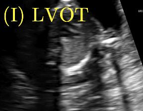
(a)

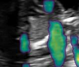
(b)

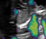
(c)

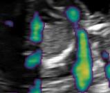
(d)

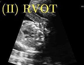
(a) Image

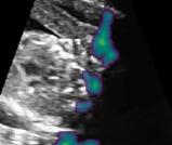
(b) Baseline

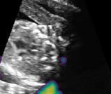
(c) Proposed

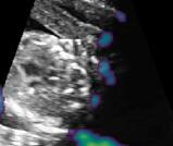
(d) Proposed$+$AG

Figure 10: Qualitative performance of our methods for detecting signal lacking regions caused by insufficient gel.

VII Conclusion

We propose a CNN-based, weakly supervised method for automatic confidence estimation of shadow regions in 2D US images. By learning and transferring shadow features from weakly-labelled images, our method can predict dense, continuous shadow confidence maps directly from input images.

We evaluate the performance of our method by comparing it to the state-of-the-art and human performance. Our experiments show that our method is quantitatively better than the state-of-the-art and human annotation for shadow segmentation. For confidence estimation of shadow regions, our method is also qualitatively better than the state-of-the-art and is more consistent than human annotation. More importantly, our method is capable of detecting disjoint multiple shadow regions without being limited by the correlation between adjacent pixels as in [16], and the heuristically selected hyperparameters in [22].

We further demonstrate that our method improves the performance of other automatic image analysis algorithms when integrating the obtained shadow confidence maps into other US applications such as standard plane classification, image fusion and automated biometric measurements.

Our method has significantly short inference time, which enables effective real-time feedback of local image properties. This feedback can guiding inexperienced sonographers to find diagnostically valuable viewing directions and pave the way for standardized image acquisition training.

-A Shadow/Shadow-free Classification Network

In this section, we use Python-inspired pseudo code to present the detailed network architecture of the shadow/shadow-free classification network (shown in Fig. 11). The conv_layer function performs a standard 2D convolution without activation layer and the global_average_pool operates spatial averaging on the feature maps. The residual_block is realized by DLTK [26].

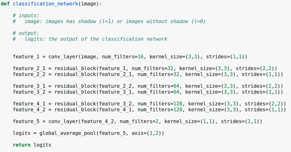
Figure 11: Shadow/shadow-free classification network architecture.

-B Shadow Segmentation Network

Fig.12 shows the detailed architecture of the segmentation network. The conv_layer function performs a standard 2D convolution without activation layer. The residual_block and the upsample_concat (the upsampling and concatenation layer) are realized by DLTK [26].

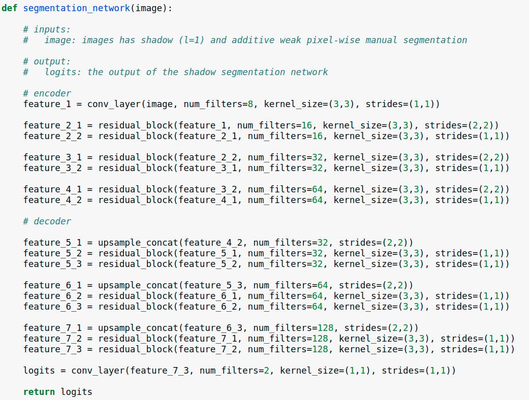
Figure 12: Shadow segmentation network architecture.

-C Confidence Estimation Network

Fig. 13 shows the detailed architecture of the shadow confidence estimation network. Similarly, the conv_layer function performs a standard 2D convolution without activation layer. The residual_block and the upsample_concat (the upsampling and concatenation layer) are realized by DLTK [26].

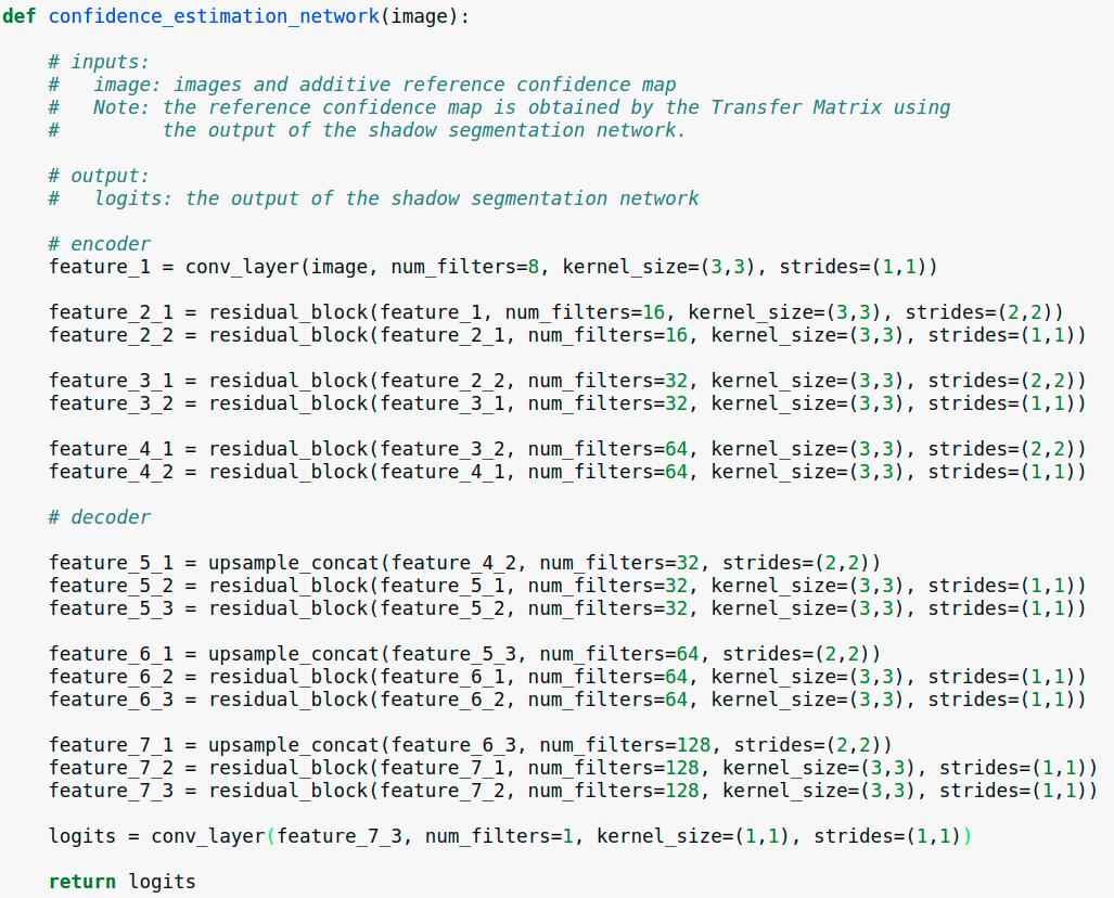
Figure 13: Shadow confidence estimation network architecture.

-D Alternative Examples of Shadow Confidence Estimation

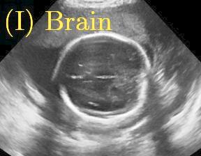
(a)

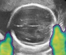
(b)

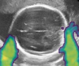
(c)

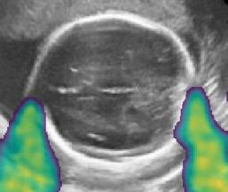
(d)

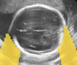
(e)

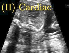
(f)

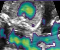
(g)

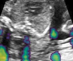
(h)

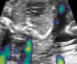
(i)

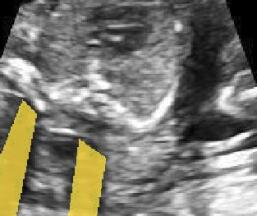
(j)

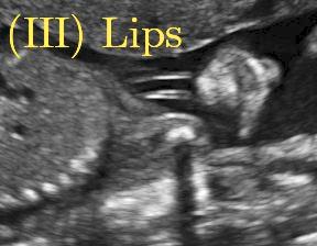
(k)

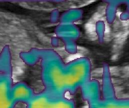
(l)

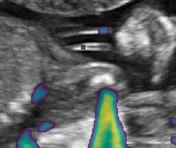
(m)

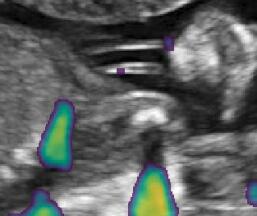
(n)

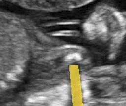
(o)

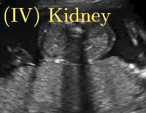
(a) Image

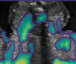
(b) Baseline

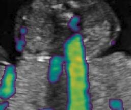
(c) Proposed

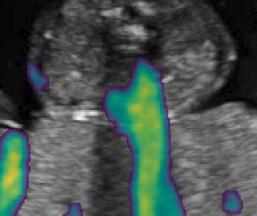
(d) Proposed$+$AG

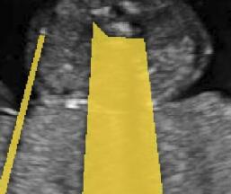
(e) Weak GT

Figure 14: Shadow confidence maps of different methods on various anatomical US images. Rows I-IV show four examples of shadow confidence estimation; Brain (top), Cardiac (middle), Lips (third) and Kidney (bottom). Columns (b-d) are shadow confidence maps from the baseline, the proposed method and the proposed method with attention gate (Proposed$+$AG). (f) is the binary map of manual segmentation.

We show an alternative group of examples for the confidence estimation of shadow regions (shown in Fig. 14). These examples include fetal brain from $M_{test}$, and cardiac, lips, kidney from $S_{test}$. Similar to the Fig. 6 in the main paper, Fig. 14 shows that the baseline fails to handle unseen data while the proposed method and the proposed$+$AG method are able to predict pixel-wise confidence of multiple shadow regions. These examples demonstrate that the shadow-seg module is able to generalize the shadow representation and transfer shadow representation from the shadow/shadow-free classification task to a confidence estimation task.

-E Data in Ultrasound Classification

Table VI shows the exact number of data used in the application of 2D US standard plane classification (Section V. Part $A$). The training data of each class is almost the same so that we can keep class balance between different classes during training.

TABLE VI: Summary of the Data Set used in Ultrasound Standard Plane Classification Task.

Class	Training	Validation	Testing
3VV	1480	50	298
4CH	1544	50	309
Abdominal	2000	50	553
Brain(Cb.)	2000	50	634
Brain(Tv.)	2000	50	899
Femur	2000	50	520
Lips	2000	50	526
LVOT	1633	50	333
RVOT	1432	50	296
Sum	16089	450	4368

-F Class Confusion Matrix

Fig. 17 additionally shows the class confusion matrix of 2D US standard plane classification in Section V. Part A. This class confusion matrix demonstrates that less 3VV images are mis-classified as RVOT images and less 4CH images are mis-classified as LVOT images after adding shadow confidence maps. However, as we discussed in the above Discuss Section, the shadow confidence maps can also introduce redundant information for similar anatomical structures in this classification task. For example, more LVOT images are wrongly classied as RVOT and more RVOT images are classified as 3VV images.

-G Examples for Image Fusion

Fig.15 shows more examples of the multi-view image fusion task which include the original multi-view images. From the column (a-b) of Fig.15, we can see that the original images contain strong shadow artifacts that can affect the anatomical analysis. The image fusion task aims to use complementary information from images with different views for reducing artifacts and increasing anatomical information. Column (e-f) enlarge the areas within the bounding boxes in column (c-d). Column (g) shows the difference masks between column (e)and (f). The difference masks clearly indicates the improved performance of image fusion after adding shadow confidence maps for Gaussian weighting strategy as well as Intensity and Gaussian weighting strategy.

(a)

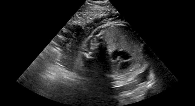
(b)

(c)

(d)

(e)

(f)

(g)

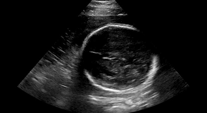
(h)

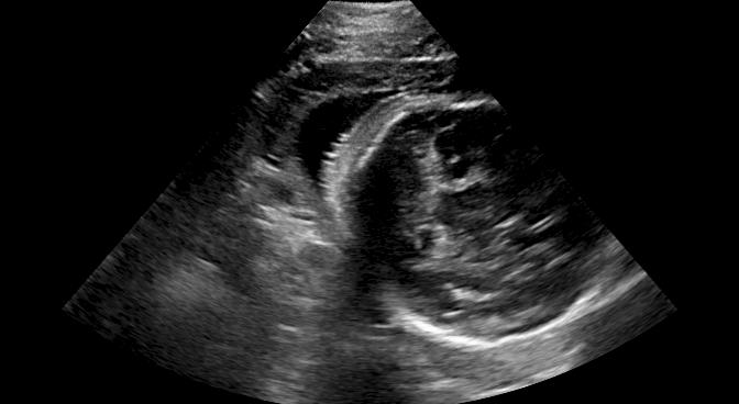
(i)

(j)

(k)

(l)

(m)

(n)

(o)

(p)

(q)

(r)

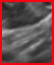
(s)

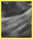
(t)

(u)

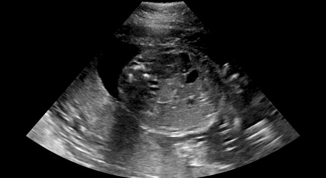
(a) Image Component 1

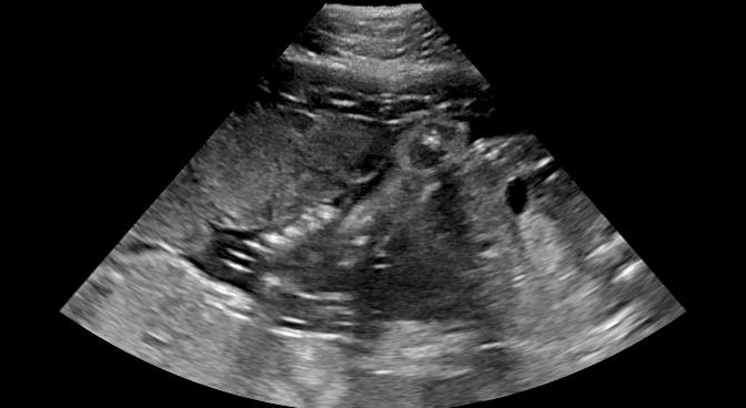
(b) Image Component 2

(c) Without ${CM}_{P}$

(d) With ${CM}_{P}$

(e) Enlarged

(f) Enlarged

(g) D$\_$map

Figure 15: The results of the multi-view image fusion. (a-b) The multi-view images, (c) Image fusion without shadow confidence maps (${CM}_{P}$), (d) Image fusion with shadow confidence maps (${CM}_{P}$), (e-f) Enlarged areas of (c-d) respectively, and (g) Difference maps of (e) and (f). Rows (1-2) use MSE loss to train networks for generating shadow confidence maps while Row (3-4) use Sigmoid loss. Row 2 uses the Gaussian weighting for image fusion while Rows (1, 3, 4) use the Intensity and Gaussian weighting. The color bar on the top shows that the more yellow/brighter, the higher the difference between the two framed areas.

-H Examples for Biometric Measurement

We visualize the biometric measurement of the three examples shown in Table V. Fig. 16 demonstrates that, for the cases affected by shadow artifacts, the segmentation performance (“EI_seg DICE”) is improved after adding shadow confidence maps as an extra channel. From the first row to the third row in Fig. 16, these three samples are respectively #1, #2 and #3 samples in Table V.

-I Equations for estimating floating point operations (Flops) for convolutional layers

We use Eq. 5 to estimate the required Flops for convolution layers including ReLU activation. Here, $W$ and $H$ are the width and height of the input image respectively. $K$ is kernel size, $P$ is the padding, $S$ is the stride and $F$ is the number of filters. $n$ is the size of the convolution layer. ($\text{channels}*K*K$).

$$\begin{split}Flops&\approx\\ &\left(\frac{W-K+2*P}{S}+1\right)*\\ &\left(\frac{H-K+2*P}{S}+1\right)*n*(n-1)*F+F*W*H.\end{split}$$ (5)

Eq. 5 evaluates the number of Flops ($n$: multiplications and $n-1$: additions) for $W\times H$ filter convolutions adjusted for padding $P$ and stride $S$. ReLU activation is assumed to be $F*W*H$ Flops (one comparison and one multiplication).

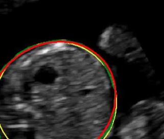
(a)

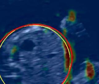
(b)

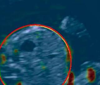
(c)

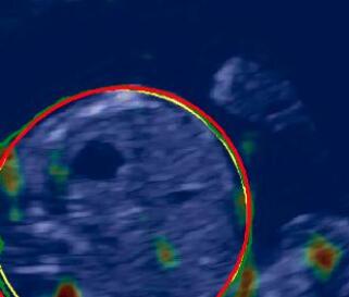
(d)

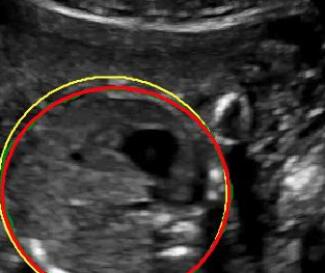
(e)

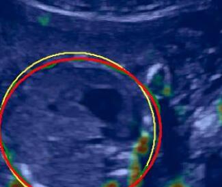
(f)

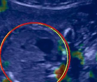
(g)

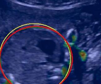
(h)

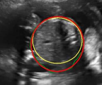
(a) w/o $CM$

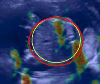
(b) ${CM}_{B}$

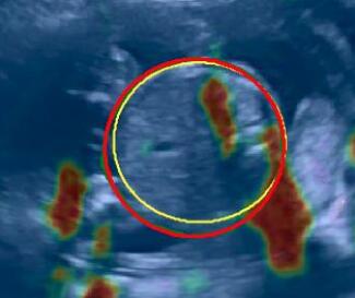
(c) ${CM}_{P}$

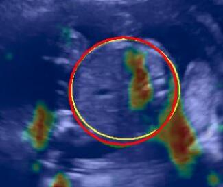
(d) ${CM}_{PAG}$

Figure 16: Biometric measurement with VS. without shadow confidence maps. The yellow circles refer to the ground truth, the green curves are segmentation predictions, and the red circles are the ellipses of the segmentation prediction.

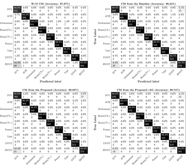
Figure 17: Class confusion metrics for 2D ultrasound standard plane classification. Upper row left: the class confusion matrix without shadow confidence maps. Upper row right: the class confusion matrix with the shadow confidence maps generated by the baseline. Lower row left: the class confusion matrix with shadow confidence maps obtained by the proposed method. Lower row right: the class confusion matrix with the shadow confidence maps produced by the proposed$+$AG method.

References

- [1] J. Abbott and F. Thurstone. Acoustic speckle: Theory and experimental analysis. Ultrasonic Imaging, 1(4):303–324, 1979.
- [2] P. Anbeek, K. L. Vincken, G. S. van Bochove, M. J. van Osch, and J. van der Grond. Probabilistic segmentation of brain tissue in mr imaging. NeuroImage, 27(4):795 – 804, 2005.
- [3] C. Baumgartner, K. Kamnitsas, J. Matthew, T. P. Fletcher, S. Smith, L. M. Koch, B. Kainz, and D. Rueckert. Sononet: Real-time detection and localisation of fetal standard scan planes in freehand ultrasound. IEEE Trans. Med. Imag., 36:2204–2215, 2017.
- [4] C. Baumgartner, L. Koch, K. Tezcan, J. Ang, and E. Konukoglu. Visual feature attribution using wasserstein gans. CoRR, abs/1711.08998, 2017.
- [5] F. Berton, F. Cheriet, M. M., and C. Laporte. Segmentation of the spinous process and its acoustic shadow in vertebral ultrasound images. Computers in Biology and Medicine, 72:201–211, 2016.
- [6] B. Bouhemad, M. Zhang, Q. Lu, and J. Rouby. Clinical review: bedside lung ultrasound in critical care practice. Critical Care, 11(1):205, 2007.
- [7] A. Broersen, M. Graaf, J. Eggermont, R. Wolterbeek, P. Kitslaar, J. Dijkstra, J. Bax, J. Reiber, and A. Scholte. Enhanced characterization of calcified areas in intravascular ultrasound virtual histology images by quantification of the acoustic shadow: validation against computed tomography coronary angiography. Int J Cardiovasc Imaging, 32:543–552, 2015.
- [8] Centre for Workforce Intelligence. Securing the future workforce supply – sonography workforce review. 2017.
- [9] H. Choi, J. Lee, S. Kim, and S. Park. Speckle noise reduction in ultrasound images using a discrete wavelet transform-based image fusion technique. Bio-Medical Materials and Engineering, 26(1):1587–1597, 2015.
- [10] P. Coupé, P. Hellier, C. Kervrann, and C. Barillot. Nonlocal means-based speckle filtering for ultrasound images. IEEE Trans. Image Process., 18(10):2221–2229, 2009.
- [11] L. R. Dice. Measures of the amount of ecologic association between species. Ecology, 26(3):297–302, 1945.
- [12] M. K. Feldman, S. Katyal, and M. S. Blackwood. Us artifacts. Radio Graphics, 29:1179–1189, 2009.
- [13] K. He, X. Zhang, S. Ren, and J. Sun. Deep residual learning for image recognition. In CVPR’16, 2016.
- [14] K. He, X. Zhang, S. Ren, and J. Sun. Identity mappings in deep residual networks. In ECCV, pages 630–645. Springer, 2016.
- [15] P. Hellier, P. Coupé, X. Morandi, and D. Collins. An automatic geometrical and statistical method to detect acoustic shadows in intraoperative ultrasound brain images. Med Image Anal, 14(2):195–204, 2010.
- [16] A. Karamalis, W. Wein, T. Klein, and N. Navab. Ultrasound confidence maps using random walks. Med Image Anal, 16(6):1101–1112, 2012.
- [17] H. Kim and T. Varghese. Hybrid spectral domain method for attenuation slope estimation. Ultrasound Med Biol, 34:1808–1819, 2008.
- [18] T. Klein and W. Wells. Rf ultrasound distribution-based confidence maps. In MICCAI’15, pages 595–602. Springer, 2015.
- [19] F. W. Kremkau and K. Taylor. Artifacts in ultrasound imaging. J Ultrasound Med, 5(4):227–237, 1986.
- [20] A. Krizhevsky, I. Sutskever, and G. Hinton. Imagenet classification with deep convolutional neural networks. In NIPS’12, pages 1097–1105, 2012.
- [21] T. Lange, N. Papenberg, S. Heldmann, J. Modersitzki, B. Fischer, H. Lamecker, and P. Schlag. 3D ultrasound-CT registration of the liver using combined landmark-intensity information. Int J Comput Assist Radiol Surg, 4(1):79–88, 2009.
- [22] Q. Meng, C. Baumgartner, M. Sinclair, J. Housden, M. Rajchl, A. Gomez, B. Hou, N. Toussaint, V. Zimmer, J. Tan, et al. Automatic shadow detection in 2d ultrasound images. In MICCAI Workshop on PIPPI, 2018.
- [23] NHS. Fetal anomaly screening programme: programme handbook June 2015. Public Health England, 2015.
- [24] J. A. Noble. Ultrasound image segmentation and tissue characterization. Proc Inst Mech Eng H., 224(2):307–316, 2010.
- [25] O. Oktay, J. Schlemper, L. L. Folgoc, M. Lee, M. P. Heinrich, K. Misawa, K. Mori, S. G. McDonagh, N. Y. Hammerla, B. Kainz, et al. Attention u-net: Learning where to look for the pancreas. CoRR, abs/1804.03999, 2018.
- [26] N. Pawlowski, S. I. Ktena, M. Lee, B. Kainz, D. Rueckert, B. Glocker, and M. Rajchl. Dltk: State of the art reference implementations for deep learning on medical images. arXiv preprint arXiv:1711.06853, 2017.
- [27] G. P. Penney, J. M. Blackall, M. S. Hamady, T. Sabharwal, A. Adam, and D. J. Hawkes. Registration of freehand 3d ultrasound and magnetic resonance liver images. Med Image Anal, 8:81–91, 2004.
- [28] M. Rajchl, M. Lee, O. Oktay, K. Kamnitsas, J. Passerat-Palmbach, W. Bai, M. Damodaram, M. Rutherford, J. Hajnal, B. Kainz, et al. Deepcut: Object segmentation from bounding box annotations using convolutional neural networks. IEEE Trans. Med. Imag., 36(2):674–683, 2017.
- [29] L. J. Salomon, Z. Alfirevic, V. Berghella, C. Bilardo, E. Hernandez-Andrade, S. L. Johnsen, K. Kalache, K. Leung, G. Malinger, H. Munoz, et al. Practice guidelines for performance of the routine mid‐trimester fetal ultrasound scan. Ultrasound Obst Gyn, 37:116–126, 2011.
- [30] T. Shen, T. Zhou, G. Long, J. Jiang, S. Pan, and C. Zhang. Disan: Directional self-attention network for rnn/cnn-free language understanding. In AAAI, 2018.
- [31] P. E. Shrout and J. L. Fleiss. Intraclass correlations: Uses in assessing rater reliability. Psychol Bull., 86(2):420–428, 1979.
- [32] M. Sinclair, C. Baumgartner, J. Matthew, W. Bai, J. Cerrolaza, Y. Li, S. Smith, C. Knight, B. Kainz, J. Hajnal, et al. Human-level performance on automatic head biometrics in fetal ultrasound using fully convolutional neural networks. In EMBC’18, 2018.
- [33] J. Springenberg, A. Dosovitskiy, T. Brox, and M. Riedmiller. Striving for simplicity: The all convolutional net. CoRR, abs/1412.6806, 2014.
- [34] R. Steel, T. L. Poepping, R. S.Thompson, and C. Macaskill. Origins of the edge shadowing artefact in medical ultrasound imaging. Ultrasound Med Biol, 39:1153–1162, 2005.
- [35] A. C. Wilson, R. Roelofs, M. Stern, N. Srebro, and B. Recht. The marginal value of adaptive gradient methods in machine learning. CoRR, abs/1705.08292, 2018.
- [36] Y. Zhang, Y. Tian, Y. Kong, B. Zhong, and Y. Fu. Residual dense network for image super-resolution. In CVPR’18, 2018.
- [37] B. Zhou, A. Khosla, A. Lapedriza, A. Oliva, and A. Torralba. Learning deep features for discriminative localization. In CVPR’16, pages 2921–2929. IEEE, 2016.
- [38] J. Zhu, T. Park, P. Isola, and A. A. Efros. Unpaired image-to-image translation using cycle-consistent adversarial networks. In ICCV’17, 2017.
- [39] A. V. Zimmer, A. Gomez, Y. Noh, N. Toussaint, B. Khanal, R. Wright, L. Peralta, V. M. Poppel, E. Skelton, J. Matthew, et al. Multi-view image reconstruction: Application to fetal ultrasound compounding. In MICCAI Workshop on PIPPI, 2018.