Topological integrability, classical and quantum chaos, and the theory of dynamical systems in the physics of condensed matter.

Abstract

The paper is devoted to the questions connected with the investigation of the S.P. Novikov problem of the description of the geometry of level lines of quasiperiodic functions on a plane with different numbers of quasiperiods. We consider here the history of the question, the current state of research in this field, and a number of applications of this problem to various physical problems. The main attention is paid to the applications of the results obtained in the field under consideration to the theory of transport phenomena in electron systems.

1 Introduction.

In this paper we will mainly consider the formulation of problems, research and results related to the S.P. Novikov problem, set in the early 1980s (see [42]) and having relation in fact to many areas of research, in particular, such as the theory of dynamical systems, the theory of quasiperiodic functions, the theory of topological phenomena in the physics of condensed matter, the theory of transport phenomena in systems of various dimensions, etc. In the very first formulation, the problem of S.P. Novikov was connected with the description of the levels of multivalued functions on manifolds, but it has the same natural formulation also in the language of the theory of dynamical systems. Most of our paper will be connected with the investigations of the Novikov problem which relate to dynamical systems arising on complex Fermi surfaces in metals in the presence of an external magnetic field. As is well known, the description of the trajectories of such systems can be effectively reduced to the description of the level lines of height functions on periodic two-dimensional surfaces embedded in three-dimensional space. More precisely, the dynamics of electron states in a crystal in the presence of an external magnetic field is described by the system (see, e.g. [1, 25, 49])

$${\dot{\bf p}}\,\,\,=\,\,\,{e\over c}\,\left[{\bf v}_{gr}\times{\bf B}\right]\,\,\,=\,\,\,{e\over c}\,\left[\nabla\epsilon({\bf p})\times{\bf B}\right]\,\,\,,$$ (1.1)

where $\,{\bf p}\,$ is the quasimomentum of the electron state. It is extremely important here that the space of quasimomenta represents actually a three-dimensional torus $\,\mathbb{T}^{3}\,$, and not the Euclidean space $\,\mathbb{R}^{3}\,$, as in the case of free electrons.

The space of electron states can also be represented as the space $\,\mathbb{R}^{3}\,$ provided that any two values of $\,{\bf p}\,$ that differ by a reciprocal lattice vector, define the same quantum-mechanical state. The function $\,\epsilon({\bf p})\,$ represents in this case a 3-periodic function in $\,\mathbb{R}^{3}\,$, and its level surfaces are two-dimensional 3-periodic surfaces in the same space. The reciprocal lattice $\,L^{*}\,$ in the quasimomentum space can be defined with the aid of its basis vectors $\,{\bf a}_{1}$, $\,{\bf a}_{2}$, $\,{\bf a}_{3}\,$, which are connected by the relations

$${\bf a}_{1}\,\,\,=\,\,\,2\pi\hbar\,\,{{\bf l}_{2}\times{\bf l}_{3}\over({\bf l}_{1},{\bf l}_{2},{\bf l}_{3})}\,\,\,,\quad{\bf a}_{2}\,\,\,=\,\,\,2\pi\hbar\,\,{{\bf l}_{3}\times{\bf l}_{1}\over({\bf l}_{1},{\bf l}_{2},{\bf l}_{3})}\,\,\,,\quad{\bf a}_{3}\,\,\,=\,\,\,2\pi\hbar\,\,{{\bf l}_{1}\times{\bf l}_{2}\over({\bf l}_{1},{\bf l}_{2},{\bf l}_{3})}$$

with the basis vectors $\,({\bf l}_{1},\,{\bf l}_{2},{\bf l}_{3})\,$ of the direct lattice of the crystal. As is not hard to see, the exact phase space then represents a torus

$$\mathbb{T}^{3}\,\,\,=\,\,\,\mathbb{R}^{3}/L^{*}\,\,\,,$$

obtained from the complete $\,{\bf p}$ - space with the aid of the factorization by the vectors

$$m_{1}\,{\bf a}_{1}\,\,\,+\,\,\,m_{2}\,{\bf a}_{2}\,\,\,+\,\,\,m_{3}\,{\bf a}_{3}\,\,\,,\quad\quad m_{1},\,m_{2},\,m_{3}\,\,\in\,\,\mathbb{Z}$$

The system (1.1) is a Hamiltonian system with the Hamiltonian $\,H\,=\,\epsilon({\bf p})\,$ and the Poisson bracket

$$\{p_{1}\,,\,p_{2}\}\,\,=\,\,{e\over c}\,B^{3}\,\,\,,\quad\{p_{2}\,,\,p_{3}\}\,\,=\,\,{e\over c}\,B^{1}\,\,\,,\quad\{p_{3}\,,\,p_{1}\}\,\,=\,\,{e\over c}\,B^{2}$$

It is easy to see that the consequence of this fact is, in particular, the conservation of the quantity $\,\epsilon({\bf p})\,$, as well as the projection of the quasimomentum on the direction $\,{\bf B}\,$, along trajectories of the system. As a consequence, geometrically the trajectories of the system (1.1) in $\,{\bf p}$ - space are actually given by the intersections of surfaces of constant energy

$$\epsilon({\bf p})\,\,\,=\,\,\,{\rm const}$$

with planes orthogonal to the magnetic field. It is also easy to see that due to this property the problem under consideration has two natural interpretations, namely, the problem of describing the trajectories of a dynamical system with an ambiguous conservation law on a compact surface and the problem of describing the level lines of a quasiperiodic function on a plane with three quasiperiods. It must be said that both these interpretations play an extremely important role in the study of the problem.

The important role of the geometry of the trajectories of the system (1.1) in the behavior of the electrical conductivity of metals in strong magnetic fields (magnetoconductivity) was first discovered by the school of I.M. Lifshits (I.M. Lifshits, M.Ya. Azbel, M.I. Kaganov, V.G. Peschanskii) in the late 1950s - early 1960s (see [26, 27, 28, 29, 30, 31, 32, 24]). We note at once that in the theory of normal metals usually only the single energy level $\,\epsilon_{F}\,$ (the Fermi level) is important for most processes occurring in metal, while all levels far from the Fermi level are always either completely filled, or empty, and do not affect the ongoing processes. As a consequence, in the theory of galvanomagnetic phenomena, only the trajectories of the system (1.1), which lie on the Fermi surface

$$S_{F}:\quad\epsilon({\bf p})\,\,\,=\,\,\,\epsilon_{F}\quad,$$

are interesting, and it is the complexity of the Fermi surface that determines the features of electron transport phenomena in strong magnetic fields.

Thus, in the paper [26] there was indicated the principal difference in the behavior of the magnetoconductivity in strong magnetic fields in the presence of only closed trajectories of the system (1.1) on the Fermi surface in $\,{\bf p}$ - space and in the presence of periodic open trajectories in $\,{\bf p}$ - space on this surface. In both cases, the asymptotic behavior of the conductivity tensor can be represented as a regular series in inverse powers of $\,B\,$, and, in particular, has the following form in the presence of only closed trajectories on the Fermi surface in $\,{\bf p}$ - space:

$$\sigma^{ik}\,\,\,\,\simeq\,\,\,\,{ne^{2}\tau\over m^{*}}\,\left(\begin{array}[]{ccc}(\omega_{B}\tau)^{-2}&(\omega_{B}\tau)^{-1}&(\omega_{B}\tau)^{-1}\cr(\omega_{B}\tau)^{-1}&(\omega_{B}\tau)^{-2}&(\omega_{B}\tau)^{-1}\cr(\omega_{B}\tau)^{-1}&(\omega_{B}\tau)^{-1}&*\end{array}\right),\quad\quad\omega_{B}\tau\,\,\rightarrow\,\,\infty$$ (1.2)

In the formula (1.2) the value $\,n\,$ represents the concentration of charge carriers in the metal, and the value $\,m^{*}\,$ determines the order of the effective mass of the electron in the crystal. The time $\,\tau\,$ plays the role of the mean free time of an electron and depends on the purity as well as the temperature of the crystal. The value $\,\omega_{B}\,=\,eB/m^{*}c\,$ has the meaning of the cyclotron frequency of the electron in the crystal, it should be noted here that, unlike the case of the free electron gas, the cyclotron frequency is defined here only for closed trajectories of the system (1.1) and coincides with the parameter $\,\omega_{B}\,$ only in order of magnitude. The sign $\,\simeq\,$ expresses here the equality up to a dimensionless coefficient (of order 1) and the notation $\,*\,$ means also some constant. Here and in what follows we will always assume that the axis $\,z\,$ in our considerations is chosen along the direction of the magnetic field. It is easy to see that the formula (1.2) coincides essentially with the analogous formula for the free electron gas, differing from it only by possible numerical parameters.

A completely different situation arises in the presence of periodic open trajectories on the Fermi surface in $\,{\bf p}$ - space. As was shown in [26], after the choice of the axis $\,x\,$ along the average direction of the periodic trajectory in $\,{\bf p}$ - space, the principal term of the asymptotic expansion of the tensor $\,\sigma^{ik}(B)\,$ can be represented in the form

$$\sigma^{ik}\,\,\,\,\simeq\,\,\,\,{ne^{2}\tau\over m^{*}}\,\left(\begin{array}[]{ccc}(\omega_{B}\tau)^{-2}&(\omega_{B}\tau)^{-1}&(\omega_{B}\tau)^{-1}\cr(\omega_{B}\tau)^{-1}&*&*\cr(\omega_{B}\tau)^{-1}&*&*\end{array}\right),\quad\quad\omega_{B}\tau\,\,\rightarrow\,\,\infty$$ (1.3)

It can be seen that the electric conductivity tensor here has a strong anisotropy in the plane orthogonal to $\,{\bf B}$ in strong magnetic fields, which makes its behavior fundamentally different from the case of the free electron gas. It is easy to see that the formula (1.3) allows also to measure the average direction of periodic trajectories in $\,{\bf p}$ - space as the direction of the greatest suppression of conductivity in the plane orthogonal to $\,{\bf B}$. Let us note here that both the closed and periodic trajectories in $\,{\bf p}$ - space are represented by closed trajectories of the system (1.1) in the torus $\,\mathbb{T}^{3}\,$. It can thus be seen that for the description of galvanomagnetic phenomena in metals, not only the shape of the trajectories of (1.1) on the Fermi surface is important, but also their homology classes under the embedding in the torus $\,\mathbb{T}^{3}$.

Quasiclassical trajectories of the system (1.1) correspond also to quasiclassical trajectories (electron packets) in the $\,{\bf x}$ - space, which are determined from the system

$${\dot{\bf x}}\,\,\,=\,\,\,{\bf v}_{gr}({\bf p})\,\,\,=\,\,\,\nabla\epsilon({\bf p})$$

The electron trajectories in $\,{\bf x}$ - space do not coincide in common with the trajectories of the system (1.1), in particular, they are not plane. However, their shape correlates quite strongly with the shape of the trajectories of (1.1). For example, the projections of the electron trajectories in the $\,{\bf x}$ - space onto the plane, orthogonal to $\,{\bf B}\,$, are similar to the corresponding trajectories of the system (1.1), rotated by $90^{\circ}$. As already noted above, the shape of the trajectories of the system (1.1) becomes important in the limit $\,\omega_{B}\tau\gg 1\,$, which can be formulated as the condition that the electron turns many times along a closed trajectory or passes a distance much greater than the size of the Brillouin zone in $\,{\bf p}$ - space between two scattering acts.

In the papers [27, 28] examples of open trajectories of a more general form on Fermi surfaces of different shapes were considered. The trajectories considered in [27, 28] are not periodic in general case, however, they also have an average direction in the plane orthogonal to $\,{\bf B}$, which also leads to a sharp anisotropy of the electric conductivity tensor in the same plane. It must be said, however, that the analytic properties of the electric conductivity tensor are generally more complex here in comparison with the case of periodic trajectories (see e.g. [24, 38]).

The problem of the complete classification of various types of trajectories of system (1.1) was first set by S.P. Novikov in the work [42] and was actively investigated in his topological school during the last decades. At present, the Novikov problem of the classification of trajectories of (1.1) (with an arbitrary dispersion law) has been studied in many details, and in particular, rather profound results have been obtained, which have already found applications in the theory of solids.

Let us note at once that the most important part of the results obtained in the investigation of Novikov’s problem was the description of stable open trajectories of the system (1.1) for an arbitrary dispersion law (A.V. Zorich, I.A. Dynnikov). The remarkable geometric properties of such trajectories made it possible to define important topological characteristics (topological quantum numbers) observable in studies of conductivity of normal metals, which, in particular, provide a convenient tool for determining the orientation of the crystal lattice in such studies (S.P. Novikov, A.Ya. Maltsev). We also note here that the description of the geometric properties of stable open trajectories of system (1.1) allows, in addition, to approach more strictly the description of the analytic properties of conductivity in strong magnetic fields in the presence of trajectories of this type.

At the same time, a detailed study of the system (1.1) has also led to the discovery of new, rather nontrivial, types of trajectories of such systems whose properties are the subject of active study at the present time. Let us note here that these trajectories exhibit very interesting (chaotic) properties both from the geometric point of view and from the point of view of the description of transport phenomena in normal metals when they appear.

We must now say that the applications of the problem of describing the trajectories of the system (1.1) are not really limited to transport phenomena in normal metals in strong magnetic fields. For example, the problem of describing the trajectories of systems similar to (1.1) also arises in the description of transport phenomena in two-dimensional electron systems placed in artificially created quasiperiodic (super)potentials in the presence of an external magnetic field. The Novikov problem is formulated here as the problem of describing the geometry of the level lines of a quasiperiodic function on a plane with a fixed number of quasiperiods. It is not difficult to see here that the problem of describing the level curves of a function with three quasiperiods (the first case following the periodic one) coincides in reality with the Novikov problem in its formulation given above. Thus, all the results obtained in the study of the trajectories of the system (1.1) are also transferred to transport phenomena in two-dimensional electron systems in superpotentials with three quasiperiods. We must note here that, unlike the situation with normal metals, the parameters of such systems are controlled in this case, which makes it possible to implement any of the cases of behavior of the system (1.1) which is interesting to us.

The problem of describing the geometry of the level lines of functions with a larger number of quasiperiods is actually much more complicated. For example, for the case of functions with four quasiperiods, a rather serious result has now been obtained (S.P. Novikov, I.A. Dynnikov), which distinguishes an important class of potentials that have topologically regular open level lines analogous to stable open trajectories of the system (1.1) in the three-dimensional case. But on the whole, the Novikov problem for four quasiperiods has been studied much less compared to the case of three quasiperiods.

Here we try to give the most complete overview of the results obtained to date and describe, as much as possible, the range of possible applications of the Novikov problem in physical problems.

2 Stable open trajectories and angular conductivity diagrams for normal metals.

In this chapter we will consider stable open trajectories of the system (1.1) and describe the main properties of transport phenomena in metals in strong magnetic fields in the presence of such trajectories on the Fermi surface. We say at once that under the stability of the open trajectories of the system (1.1) we mean here the preservation of such trajectories, as well as their geometric properties, for all small variations in the direction of $\,{\bf B}\,$ or the energy level $\,\epsilon({\bf p})\,=\,\epsilon_{0}\,$. We also note that we consider the system (1.1) in the covering space of quasimomenta, where geometrically its trajectories are given by the intersections of surfaces of constant energy and planes orthogonal to the magnetic field. As we said above, the dispersion relation $\,\epsilon({\bf p})\,$ is assumed here to be an arbitrary smooth 3-periodic function in the $\,{\bf p}$ - space, with periods equal to the vectors of the reciprocal lattice.

Let us describe here two important properties of stable open trajectories of the system (1.1), which follow from the results obtained in the papers [50, 14, 15].

1) All stable open trajectories of the system (1.1) for a fixed direction of $\,{\bf B}\,$ lie in straight strips of finite width in planes orthogonal to $\,{\bf B}\,$, passing through them (Fig. 1).

2) All stable open trajectories of the system (1.1) for a fixed direction of $\,{\bf B}\,$ have the same mean direction in $\,{\bf p}$ - space defined by the intersection of the plane orthogonal to $\,{\bf B}\,$ with some integral (generated by two vectors of the reciprocal lattice) plane $\,\Gamma\,$, unchanged for all close directions of $\,{\bf B}\,$.

Figure 1: The form of a stable open trajectory in the plane, orthogonal to $\,{\bf B}\,$, in the space of quasimomenta.

In a more precise formulation, it follows from the papers [50, 14] that the properties (1)-(2) hold for open trajectories of (1.1) for the directions of $\,{\bf B}\,$, sufficiently close to rational directions, while it follows from the paper [15] that properties (1)-(2) hold for open trajectories that are stable with respect to variations of the energy level $\,\epsilon({\bf p})\,=\,\epsilon_{0}\,$. It is not difficult to see here that to satisfy conditions (1)-(2) it is sufficient to require either the stability of trajectories with respect to small rotations of the direction of $\,{\bf B}\,$, or stability with respect to variations of the energy level. Let us also note here that property (1) was first expressed by S.P. Novikov in the form of a conjecture, and was thus proved later for stable open trajectories of (1.1).

Conditions (1) and (2) play an important role for transport phenomena in metals and served as the basis for introducing in [43] (see also [44]) important topological characteristics (topological quantum numbers) observable in magnetic conductivity in the presence of stable open trajectories on the Fermi surface. Thus, the fulfillment of conditions (1) and (2) leads to a strong anisotropy of the conductivity in the plane orthogonal to $\,{\bf B}\,$ in the limit $\,\omega_{B}\tau\gg 1\,$, which makes it possible to measure the average direction of stable open trajectories with direct measurement of conductivity in strong magnetic fields. It should be noted here that the analytic behavior of the conductivity is, in general, more complicated than the dependence (1.3) in this situation (see [38]), but in any case, we have here the relations

$$\sigma^{ik}\,\,\,\,\simeq\,\,\,\,{ne^{2}\tau\over m^{*}}\,\left(\begin{array}[]{ccc}o(1)&o(1)&o(1)\cr o(1)&*&*\cr o(1)&*&*\end{array}\right),\quad\quad\omega_{B}\tau\,\,\rightarrow\,\,\infty$$ (2.1)

provided that the axis $\,x\,$ coincides with the mean direction of the open trajectories in the $\,{\bf p}$ - space. Thus, the mean direction of stable open trajectories in $\,{\bf p}$ - space is directly observable as the direction of the largest suppression of conductivity in the plane orthogonal to $\,{\bf B}$ in strong magnetic fields. Variations of the direction of the magnetic field within the stability zone for the given family of open trajectories determine, in this case, the direction of the integral plane $\,\Gamma\,$ in $\,{\bf p}$ - space associated with this family according to condition (2).

We note here that the plane $\,\Gamma\,$ is integral in the space of quasimomenta, which means that it is generated by some two vectors of the reciprocal lattice. In particular, it does not have to coincide in the general case with any of the crystallographic planes in the coordinate space. Instead, it can be given in coordinate space by the relation

$$M_{1}\,\left({\bf x},{\bf l}_{1}\right)\,\,+\,\,M_{2}\,\left({\bf x},{\bf l}_{2}\right)\,\,+\,\,M_{3}\,\left({\bf x},{\bf l}_{3}\right)\,\,\,=\,\,\,0\,\,\,,\quad\quad M_{1},M_{2},M_{3}\,\in\,\mathbb{Z}$$

and, thus, is orthogonal to one of the integer crystallographic directions. The irreducible integer triple $\,(M_{1},M_{2},M_{3})\,$ represents here a topological characteristic of the corresponding family of stable open trajectories that is directly observable in conductivity measurements in strong magnetic fields. Integral triples $\,(M^{\alpha}_{1},M^{\alpha}_{2},M^{\alpha}_{3})\,$ for the complete set of all different Stability Zones $\,\Omega_{\alpha}\,$ in the space of directions of $\,{\bf B}\,$ were called in [43] the topological quantum characteristics (topological quantum numbers) observable in the conductivity of normal metals.

It can thus be seen that the measurement of the conductivity for different directions of $\,{\bf B}\,$ within the same Stability Zone $\,\Omega_{\alpha}\,$ allows us to determine quite accurately some (known) crystallographic direction in the coordinate space. The same conductivity measurement for the directions of $\,{\bf B}$ lying in two different Stability Zones (with different topological quantum numbers) makes it possible to completely determine the orientation of the crystal lattice of a single crystal. Let us note here that such a method of determining the orientation of a single crystal sample is significantly more convenient than, for example, the measurement of the exact angular diagram of conductivity, since (as we shall see below) the exact boundaries of the Stability Zones are actually difficult to observe in direct conductivity measurements (see, e.g. [38, 39]), and also because precise determination of the theoretical boundaries of the Stability Zones for a given dispersion relation is also a serious task in the general case (see [7]).

Stability Zones represent domains with piecewise smooth boundaries in the space of directions of $\,{\bf B}\,$ (on the unit sphere $\,\mathbb{S}^{2}$). The full Stability Zone $\,\Omega_{\alpha}\,$ can be defined as a complete domain on the sphere $\,\mathbb{S}^{2}\,$ such that for any direction $\,{\bf B}\,\in\,\Omega_{\alpha}\,$ there are stable open trajectories on the Fermi surface that correspond to the same topological quantum numbers $\,(M^{\alpha}_{1},M^{\alpha}_{2},M^{\alpha}_{3})$. It is easy to see that the full Stability Zone is invariant under the substitution $\,{\bf B}\,\rightarrow\,-{\bf B}\,$ and often consists of two opposite connected components on the unit sphere.

The addition to the union of the bands $\,\Omega_{\alpha}\,$ on the unit sphere

$$\hat{S}^{2}\,\,\,=\,\,\,\mathbb{S}^{2}\setminus\cup\Omega_{\alpha}$$

is by definition the set of directions of $\,{\bf B}\,$ for which stable open trajectories are not present on the Fermi surface. At the same time, however, the set $\,\hat{S}^{2}\,$ can contain directions of $\,{\bf B}$, corresponding to the appearance of unstable open trajectories of the system (1.1) on the Fermi surface. Among such directions, we should especially note the directions of $\,{\bf B}$, which lead to the appearance of periodic open trajectories on the Fermi surface that are unstable for $\,{\bf B}\,\in\,\hat{S}^{2}\,$. The presence of a large number of such directions of $\,{\bf B}\,$ on the set $\,\hat{S}^{2}\,$ is in fact a consequence of the topological structure of the system (1.1) for $\,{\bf B}\,\in\,\Omega_{\alpha}\,$, which we briefly describe below.

The topological structure of the system (1.1) in the presence of stable open trajectories was described in the papers [50, 15] and is based on a property that can be called “topological integrability” for systems of this type. Namely, consider the system (1.1) on a fixed surface $\,\epsilon({\bf p})\,=\,{\rm const}\,$. Let us assume that the direction of $\,{\bf B}\,$ has maximal irrationality and remove from this surface all closed trajectories of the system (1.1) (homologous to zero in the torus $\,\mathbb{T}^{3}$). It is not difficult to see that the remainder of the surface will be the carrier of the open trajectories of the system (1.1). As follows from the works [50, 15], in the presence of stable open trajectories of the system (1.1) on the surface, each connected component of such a carrier represents a two-dimensional torus $\,\mathbb{T}^{2}\,$ with contractible holes embedded in the torus $\,\mathbb{T}^{3}$.

Returning to the covering $\,{\bf p}$ - space, we can thus say that any connected component of the energy (Fermi) surface carrying stable open trajectories of the system (1.1) has a well-defined topological structure, defined by the trajectories of the system (1.1). Namely, each such connected component represents a union of integral (periodically deformed) planes in the $\,{\bf p}$ - space connected by parts formed by cylinders of closed trajectories of the system (1.1). It can be noted here also that for almost any real dispersion law the corresponding parts will in fact be simple cylinders of closed trajectories bounded by singular trajectories on their bases (Fig. 2).

Figure 2: Structure of a connected component of the Fermi surface carrying stable open trajectories of the system (1.1) in the covering $\,{\bf p}$ - space.

The results of investigations of the Novikov problem in solid state theory are most significant in cases when the dispersion relation for the electron in a crystal has a rather complex form. In particular, this refers to the shape of the Fermi surface, which is also assumed here to be quite complicated. We can say, for example, that a metal has a complex Fermi surface $\,S_{F}$, if it has rank 3, where the rank of the surface is determined by the dimension of the image of the mapping

$$H_{1}(S_{F})\,\,\,\rightarrow\,\,\,H_{1}(\mathbb{T}^{3})$$

It can also be seen that a connected Fermi surface of rank 3 must necessarily have genus $\,g\,\geq\,3$.

Thus, according to the introduced terminology, a complex connected component of the Fermi surface, having the structure shown at Fig. 2, must contain at least two nonequivalent families of parallel planes connected by cylinders of closed trajectories of both “electron” and “hole” type. In the general case, as is not hard to see, the number of nonequivalent integral planes in this representation of the Fermi surface is necessarily even, and the corresponding planes can be divided into two classes in accordance with the direction of motion (“forward” or “back”) along the corresponding open trajectories in $\,{\bf p}$ - space. It can also be noted that for the overwhelming number of real crystals, the number of nonequivalent integral planes in the described representation is exactly two, since a larger number of such planes corresponds to rather large genera of the Fermi surface. Based on the form of real dispersion relations, it is this situation, therefore, that should be considered typical when stable open trajectories of the system (1.1) appear on the Fermi surface. We also note here that the structure shown at Fig. 2 has a purely topological character and can be visually much more complicated for real Fermi surfaces.

It is not difficult to see that the presence of at least one pair of carriers of stable open trajectories excludes the appearance of open trajectories of the system (1.1) having a different form, and that all the present open trajectories have the same direction in the $\,{\bf p}$ - space in this case. We note that this property is also true for Fermi surfaces consisting of several connected components (in the torus $\,\mathbb{T}^{3}$), provided that these components do not intersect each other. This circumstance is especially important for Fermi surfaces of real crystals, which usually consist of several components, determined by different dispersion relations (the property of non-intersection of different components of the Fermi surface is, as a rule, preserved in this case). This property of stable open trajectories for the full Fermi surface was called the Topological Resonance in [34, 35] and plays an important role in describing angular diagrams for conductivity in real conductors. In particular, this property excludes the possibility of crossing two Stability Zones with different topological quantum numbers on the angular diagram.

It is easy to see also, that in the situation described above the open trajectories of the system (1.1) exist on all the presented integral planes for all directions of $\,{\bf B}$, except possibly for the direction orthogonal to the plane $\,\Gamma_{\alpha}$ (if this direction belongs to the Zone $\,\Omega_{\alpha}$). It can also be seen that the described structure of the Fermi surface is preserved under rotations of the direction of $\,{\bf B}\,$ as long as all the cylinders of closed trajectories connecting the integral planes remain unbroken. The boundary of the corresponding Stability Zone on the angular diagram is thus determined by the condition that the height of one of the cylinders of closed trajectories described above (Fig. 3) goes to zero.

Figure 3: The vanishing of the height of one of the cylinders of closed trajectories of the system (1.1), followed by a “jump” of trajectories from one integral plane to another when crossing the boundary of a Stability Zone on the angular diagram.

It is not difficult to see that the total boundary of a Stability Zone on the angular diagram can be either “simple” and correspond to the disappearance of only one cylinder of closed trajectories (Fig. 4), or “compound” and be determined by the disappearance of different cylinders of closed trajectories in its different parts (Fig. 5). Besides that, it is also easy to see that in the case of a compound boundary of a Stability Zone we can have cases when the cylinders of different (electron and hole) types disappear in different parts of the boundary (Fig. 5), and when different cylinders of the same type disappear in its different parts (Fig. 6).

Figure 4: The Fermi surface having a Stability Zone $\,\Omega_{\alpha}\,$ with a simple boundary.

Figure 5: The Fermi surface having a Stability Zone $\,\Omega_{\alpha}\,$ with a compound boundary.

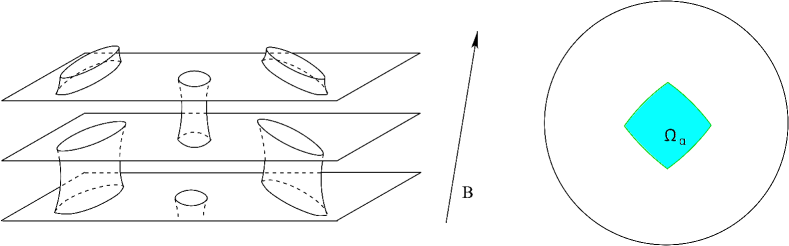
Figure 6: The Fermi surface having a Stability Zone $\,\Omega_{\alpha}\,$ with a compound boundary, determined by the disappearance of different cylinders of the same type in its different parts.

What also can be noted in the situation described above is that the representation of the Fermi surface, shown at Fig. 2, allows actually to give an effective description of the trajectories of the system (1.1) also immediately after crossing the boundary of the Stability Zone $\,\Omega_{\alpha}\,$ on the angular diagram. Indeed, after the intersection of the boundary of $\,\Omega_{\alpha}\,$ the trajectories can jump between the previous carriers of open trajectories, however, the Fermi surface is still divided into pairs of such carriers separated from each other by the remaining cylinders of closed trajectories. It can be seen in this case that the corresponding component is completely divided into closed trajectories if the intersection of the plane orthogonal to $\,{\bf B}$ with the plane $\,\Gamma_{\alpha}\,$ has an irrational direction, and can contain open periodic trajectories if this intersection has a rational direction in the $\,{\bf p}$ - space. It is also easy to see that the resulting closed trajectories are strongly elongated in one direction and have very long length, so that in the immediate vicinity of the boundary of $\,\Omega_{\alpha}\,$ we have the relation $\,T\,\geq\,\tau\,$, where $\,T\,$ is the typical time of a turn along such trajectories. As a consequence, trajectories of this type are indistinguishable from open trajectories from the experimental point of view, and the exact boundary of the Zone $\,\Omega_{\alpha}\,$ is actually unobservable in direct conductivity measurements even in rather strong magnetic fields. Besides that, when approaching the boundary of the Zone $\,\Omega_{\alpha}\,$ from the outside, there will be more and more directions of $\,{\bf B}$, corresponding to the presence of periodic open trajectories on pairs of former carriers of stable open trajectories of system (1.1). It can thus be stated that for direct conductivity measurements the “experimentally observable” Stability Zone $\,\hat{\Omega}_{\alpha}\,$ does not coincide with the exact mathematical Stability Zone $\,\Omega_{\alpha}\,$ and contains it as a subset (Fig. 7). It must be said that the analytic dependence of the tensor $\,\sigma^{ik}({\bf B})\,$ both on the direction and on the value of $\,{\bf B}\,$ inside the Zone $\,\hat{\Omega}_{\alpha}\,$ is generally quite complicated and can be approximated by different regimes in its different parts (see [38]). Let us also note here that the analytic properties of the tensor $\,\sigma^{ik}({\bf B})\,$ in the Zones $\,\hat{\Omega}_{\alpha}\,$ can play, presumably, a certain role in considering the conductivity of polycrystals in strong magnetic fields (see, e.g. [12, 13]), which also possesses rather non-trivial properties in metals with complex Fermi surfaces. At the same time, in spite of the unobservability of the exact boundaries of the Stability Zones in direct conductivity measurements, it is nevertheless possible to indicate other experimental methods that allow one to determine the exact mathematical Stability Zones for real materials. In particular, as can be shown, this problem can be solved using the study of classical or quantum oscillation phenomena (cyclotron resonance, de Haas - van Alphen effect, Shubnikov - de Haas effect, etc.) in strong magnetic fields (see [39]).

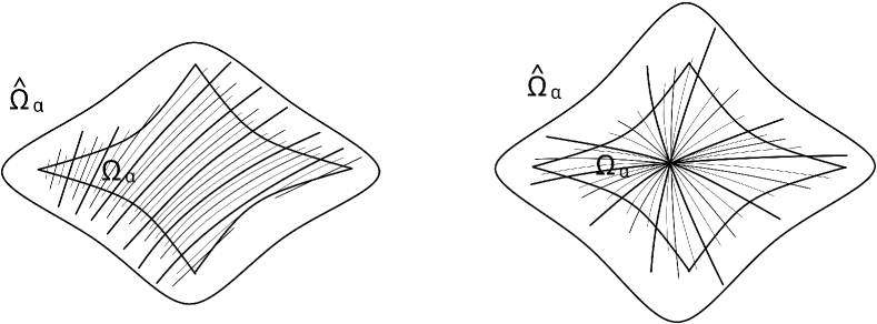
Figure 7: A schematic view of the experimental Stability Zones $\,\hat{\Omega}_{\alpha}\,$ observable in direct measurements of conductivity in strong magnetic fields (the “nets” of special directions of $\,{\bf B}$, corresponding to the appearance of periodic trajectories on the Fermi surface, are also shown).

As also follows from the arguments of the previous paragraph, each Stability Zone $\,\Omega_{\alpha}\,$ is in fact surrounded by some additional domain $\,\Omega^{\prime}_{\alpha}\,$, restricted by some “second boundary” of the Stability Zone, determined by the disappearance of at least one more cylinder of closed trajectories presented at Fig. 2. Everywhere in the region $\,\Omega^{\prime}_{\alpha}\,$ the Fermi surface can be represented as a union of pairs of former carriers of stable open trajectories admitting jumps of the trajectories of the system (1.1), separated by the remaining cylinders of closed trajectories. It is easy to see that in the most common case we are considering (exactly two carriers of open trajectories in the Zone $\,\Omega_{\alpha}$), in the domain $\,\Omega^{\prime}_{\alpha}\,$ there can be no open trajectories other than (unstable) periodic trajectories whose direction is determined by the same rule as the mean direction of the open trajectories in the Zone $\,\Omega_{\alpha}$. It must be said that for Fermi surfaces of very high genus (more than two carriers of open trajectories in the Zone $\,\Omega_{\alpha}$), of course, we can have the situation when the “merged” carriers of open trajectories coexist with unbroken carriers having the same direction in $\,{\bf p}$ - space. In this case, one can speak of a Stability Zone with a complex boundary or of the imposition of Stability Zones corresponding to the same topological quantum numbers. The region $\,\Omega^{\prime}_{\alpha}\,$ can be called the “derivative” of the Stability Zone $\,\Omega_{\alpha}$, since the structure of the system (1.1) in this region is closely related to the structure of the same system in the Zone $\,\Omega_{\alpha}$. It is easy to see that, like the first boundary of the Stability Zone, its second boundary can also be either simple or compound in the sense indicated above (Fig. 8). It can also be seen that for any connected part of the region $\,\Omega^{\prime}_{\alpha}\,$ its inner (bordering $\,\Omega_{\alpha}$) and outer boundaries correspond to the disappearance of the cylinders of closed trajectories of the opposite (electron and hole) types at Fig. 2. We also note here that for a precise determination of the second boundaries of the Stability Zones in real crystals, we can also propose a number of experimental methods, including the study of classical or quantum oscillations in strong magnetic fields mentioned earlier (see [40]).

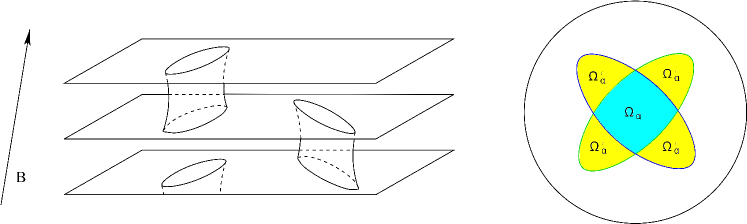
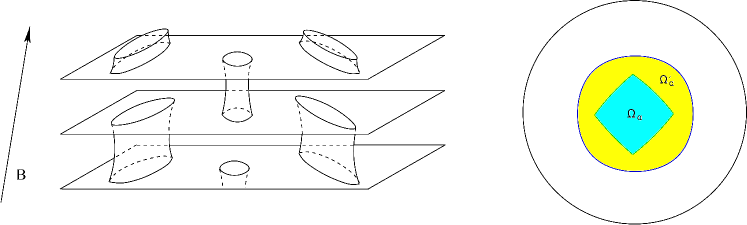
Figure 8: The second boundaries of the Stability Zones, bounding the domains $\,\Omega^{\prime}_{\alpha}\,$.

It should also be noted that the type of cylinder of closed trajectories disappearing at any of the sections of the (first) boundary of a Stability Zone is also observable experimentally and, moreover, plays an important role in the conductivity behavior outside of $\,\Omega_{\alpha}$. Namely, it can be shown that the type of the vanishing cylinder determines the behavior of the Hall conductivity in strong magnetic fields in that part of the region $\,\Omega^{\prime}_{\alpha}\,$, where the condition $\,\tau\,\gg\,T\,$ starts to be fulfilled. Let us note at once that the behavior of the Hall conductivity in this limit is usually associated with the concentration of electron and hole carriers in a conductor, however, the type of current carriers is not determined in the presence of open trajectories of the system (1.1) on the Fermi surface. Let us consider here for simplicity (the most realistic) the case when the connected component of the Fermi surface carrying stable open trajectories has exactly two nonequivalent carriers of open trajectories. In this case it can be shown (see [40]) that in calculating the Hall conductivity in the indicated part of $\,\Omega^{\prime}_{\alpha}\,$ one can assume that such a component is bounding either the carriers of the electron type, or carriers of the hole type, depending on the type of the vanishing cylinder of closed trajectories on the corresponding part of the boundary of $\,\Omega_{\alpha}$. More precisely, the connected component must be regarded as bounding carriers of the electron type if on the corresponding part of the boundary of $\,\Omega^{\prime}_{\alpha}\,$ and $\,\Omega_{\alpha}\,$ we observe disappearance of a cylinder of closed hole-type trajectories, and bounding carriers of the hole type in the opposite case. To calculate the contribution of such a component to the Hall conductivity in the limit $\,\tau\,\gg\,T\,$, one can use one of the formulas

$$\sigma^{12}\,\,\,=\,\,\,{2ec\over(2\pi\hbar)^{3}B}\,\,\,V_{-}\quad\quad{\rm(\text{the first case})}$$ (2.2)

$$\sigma^{12}\,\,\,=\,\,\,-\,{2ec\over(2\pi\hbar)^{3}B}\,\,\,V_{+}\quad\quad{\rm(\text{the second case})}$$ (2.3)

where $\,V_{-}\,$ and $\,V_{+}\,$ represent the volumes of the regions bounded by the component under consideration (in the Brillouin zone) and determined by conditions $\,\epsilon({\bf p})\,<\,\epsilon_{F}\,$ and $\,\epsilon({\bf p})\,>\,\epsilon_{F}\,$ respectively. (To calculate the total Hall conductivity, it is necessary to carry out summation over all connected components of the Fermi surface).

Let us recall here that the Hall conductivity represents a “transverse” conductivity in the plane orthogonal to the magnetic field, and traditionally has a positive sign for positively charged current carriers and negative for negatively charged ones in strong magnetic fields (electron charge $\,e\,$ is assumed to be negative here). As we have already mentioned, for conductors with Fermi surfaces of general form, the carrier charge must be effectively considered positive or negative, depending on the trajectories of the system (1.1). The type of current carriers is usually well defined for metals with simple Fermi surfaces (of rank zero) that admit only closed trajectories of the system (1.1), and does not depend in this case on the direction of the magnetic field. At the same time, for metals with complex Fermi surfaces, the carrier type is not defined for the directions of $\,{\bf B}\,$ lying in the Stability Zones, as mentioned above. At the same time, the type of carriers can be defined for directions of $\,{\bf B}\,$ lying outside any of the Stability Zones, when the Fermi surface contains only closed trajectories of the system (1.1), and this property is stable with respect to small rotations of $\,{\bf B}\,$. (Let us note here that this fact does not actually mean the existence of closed trajectories of the system (1.1) of a fixed type (electron or hole) on each of the components of the Fermi surface. Nevertheless, although on any part of the Fermi surface in this case there can be closed trajectories of both types, it is possible to effectively assign to it a fixed number of carriers of a certain type (in the Brillouin zone) by relating the number of carriers to one of the volumes bounded by the corresponding component of the Fermi surface.) As follows from the formulas (2.2), (2.3), the value of the Hall conductivity is then locally constant (for a fixed value of $\,B$) under the condition $\,\tau\,\gg\,T\,$. It can be seen that in this case it is natural to divide the angular diagrams for conductivity into two classes, namely, to diagrams for which the carriers have the same charge (type A) everywhere outside the Stability Zones, and diagrams for which in different regions outside the Stability Zones carriers have different charge (type B).

We must at once say that diagrams of type A are a priori simpler and, moreover, appear, apparently, in most of the cases when studying the conductivity of real crystalline conductors. In particular, such diagrams include all diagrams containing only a finite (or infinite) number of Stability Zones that do not divide the sphere $\,\mathbb{S}^{2}\,$ into unrelated domains. As for the B-type diagrams, it is easy to see that the Stability Zones should form a rather complex structure here, splitting $\,\mathbb{S}^{2}\,$ into regions with different types of current carriers. Nevertheless, from a theoretical point of view, B-type diagrams also represent general diagrams, and in particular arise each time when there is at least one Stability Zone with a compound boundary defined by the disappearance of cylinders of closed trajectories of different types on its different parts (Fig. 5). As already noted above, in this case we necessarily have a situation when in different parts of the region $\,\Omega^{\prime}_{\alpha}\,$ the corresponding component of the Fermi surface corresponds to carriers of different types for generic directions of $\,{\bf B}$. It can also be noted that the type of carriers does not change in generic case also after crossing the second boundary of a Stability Zone (see [40]), so that the regions of different types of charge carriers that arise in this case have a rather complex structure, separated by “chains” of Stability Zones on $\,\mathbb{S}^{2}\,$ (Fig. 9). Note also that the “chains” contain generically an infinite number of Stability Zones. Thus, for example, the “corner” point of the Stability Zone at Fig. 5 can be adjoined by another Stability Zone only if the corresponding direction of $\,{\bf B}\,$ is associated with the appearance of periodic open trajectories on the Fermi surface. In the case of a general position the corner point of the Zone at Fig. 5 must be adjoined by a chain of an infinite number of decreasing Stability Zones.

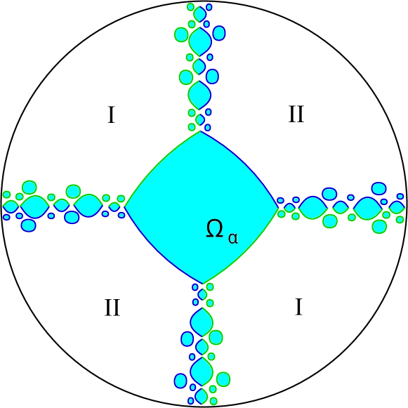
Figure 9: The angular diagram of type B and the Stability Zones separating regions corresponding to different values of the Hall conductivity on $\,\mathbb{S}^{2}\,$ (schematically, only the mathematical boundaries of a finite number of exact Stability Zones are shown).

As we have already said, diagrams of type A are, apparently, the main type that arises for real crystal conductors. At the same time, the detection of a B-type diagram for some real material would allow us to observe a wide variety of different behavior regimes for the magnetoconductivity for different directions of $\,{\bf B}\,$. It can be noted at the same time that despite the possible experimental difficulties in observing the entire complex picture of the Stability Zones arising in this case, the identification of the type of the diagram can be easily established by the behavior of the Hall conductivity outside the (experimentally observable) Stability Zones. We note here that, since the total Fermi surface can consist of several components that contribute to the Hall conductivity, a B-type diagram differs in the general case by the presence of at least two different values of Hall conductivity (no matter what sign) in different domains outside the experimentally observable Stability Zones at a given value of $\,B$.

We can also define extended Stability Zones

$$\Sigma_{\alpha}\,\,\,=\,\,\,\Omega_{\alpha}\,\cup\,\Omega^{\prime}_{\alpha}\quad,$$

defined by the union of domains $\,\Omega_{\alpha}\,$ and $\,\Omega^{\prime}_{\alpha}\,$. It is not difficult to see then that the open trajectories of the system (1.1), other than those considered above, can arise only on the set

$$\mathbb{S}^{2}\,\setminus\,\cup_{\alpha}\bar{\Sigma}_{\alpha}$$

of directions of $\,{\bf B}\,$ on the angular diagram. We note here that the size and shape of the extended Stability Zones are not related in general to the size of the experimentally observable Stability Zones $\,\hat{\Omega}_{\alpha}\,$, so that the Zones $\,\Sigma_{\alpha}\,$ can be both subsets of $\,\hat{\Omega}_{\alpha}\,$, or contain $\,\hat{\Omega}_{\alpha}\,$ as subsets. Note also that, unlike Zones $\,\Omega_{\alpha}\,$, the Zones $\,\Sigma_{\alpha}\,$ can overlap with each other. In particular, if the Zones $\,\Sigma_{\alpha}\,$ cover the entire sphere $\,\mathbb{S}^{2}\,$, this means that on the given Fermi surface only stable or periodic open trajectories of the system (1.1) can appear.

Thus, in the most general case, on the angular diagram of conductivity we can have a finite or infinite number of disjoint mathematical Stability Zones $\,\Omega_{\alpha}\,$ corresponding to different topological numbers $\,(M^{\alpha}_{1},M^{\alpha}_{2},M^{\alpha}_{3})\,$ and covering some part of the sphere $\,\mathbb{S}^{2}\,$. On the remaining part of $\,\mathbb{S}^{2}\,$ for almost all directions of $\,{\bf B}\,$ the Fermi surface contains only closed trajectories of the system (1.1). For special directions of $\,{\bf B}\,$, nevertheless, unstable periodic trajectories of the system (1.1) or chaotic trajectories of Tsarev or Dynnikov type (they will be considered in the next chapter) may appear on the Fermi surface. As we have already said, theoretically, all the angular diagrams of conductivity can be divided into two types A and B. The diagrams of the second type differ in this case by the presence of regions outside the Stability Zones with different values of the Hall conductivity in strong magnetic fields and an infinite number of Stability Zones $\,\Omega_{\alpha}\,$ (generically) which divide these regions in the general case. As we have already noted, in the experiments on direct measurement of the magnetoconductivity, the exact mathematical Stability Zones are usually included in the wider “experimentally observable” Stability Zones $\,\hat{\Omega}_{\alpha}\,$. In addition, as was also noted above, for each Stability Zone $\,\Omega_{\alpha}\,$ we can indicate an adjoining domain $\,\Omega^{\prime}_{\alpha}\,$, where the description of trajectories of the system (1.1) is actually closely related to the structure of (1.1) in the Zone $\,\Omega_{\alpha}\,$ and does not allow the appearance of open trajectories of (1.1), other than periodic. We note here again that the described structure of the angular diagram of conductivity holds for all Fermi surfaces (not necessarily defined by a single dispersion relation) consisting of components that do not intersect each other.

Returning to the general problem of describing the geometry of the trajectories of the system (1.1) with an arbitrary dispersion law, it is also necessary to give a description of the angular diagrams for the total dispersion relation $\,\epsilon({\bf p})\,$, introduced by I.A. Dynnikov in the work [18]. Let us formulate here the main statements given in [18], which represent a basis for describing such diagrams.

Consider an arbitrary dispersion relation given by a smooth 3-periodic function $\,\epsilon({\bf p})\,$, such that $\,\epsilon_{min}\,\leq\,\epsilon({\bf p})\,\leq\,\epsilon_{max}\,$. Let us fix an arbitrary direction of $\,{\bf B}\,$ and consider the energy levels $\,\epsilon({\bf p})\,=\,const\,$ containing open trajectories of the system (1.1) in the extended $\,{\bf p}$ - space.

Then:

Energy levels containing open trajectories of (1.1) represent either a connected interval

$$\epsilon_{1}({\bf B}/B)\,\,\,\leq\,\,\,\epsilon\,\,\,\leq\,\,\,\epsilon_{2}({\bf B}/B)$$

or only one isolated point $\,\epsilon\,=\,\epsilon_{0}({\bf B}/B)$.

For generic directions of $\,{\bf B}\,$ the boundaries of the interval of open trajectories $\,\epsilon_{1}({\bf B}/B)\,$ and $\,\epsilon_{2}({\bf B}/B)\,$ are determined by the values of some globally defined continuous functions $\,\tilde{\epsilon}_{1}({\bf B}/B)\,$ and $\,\tilde{\epsilon}_{2}({\bf B}/B)\,$. At the same time, for special directions of $\,{\bf B}\,$, corresponding to appearance of periodic open trajectories of system (1.1), we can write the relations

$$\epsilon_{1}({\bf B}/B)\,\,\,\leq\,\,\,\tilde{\epsilon}_{1}({\bf B}/B)\,\,\,,\quad\epsilon_{2}({\bf B}/B)\,\,\,\geq\,\,\,\tilde{\epsilon}_{2}({\bf B}/B)$$ (2.4)

Every time when we have the situation $\,\tilde{\epsilon}_{2}({\bf B}/B)\,>\,\tilde{\epsilon}_{1}({\bf B}/B)\,$, all the (non-singular) open trajectories of system (1.1), arising for generic directions of $\,{\bf B}\,$, have a regular shape, represented at Fig. 1, and the same mean direction given by the intersection of the plane orthogonal to $\,{\bf B}\,$ and some integral plane $\,\Gamma\,$ in the $\,{\bf p}$ - space.

All such trajectories, arising for generic directions of $\,{\bf B}\,$, and also the integral plane $\,\Gamma\,$ are stable with respect to small rotations of $\,{\bf B}\,$, and the complete set of directions of $\,{\bf B}\,$, corresponding to the same plane $\,\Gamma\,$, represents a finite domain with piecewise smooth boundary on the angular diagram $\,\mathbb{S}^{2}$. The regions $\,\Omega^{*}_{\alpha}\,$, corresponding to the presence of stable open trajectories with the same integral plane $\,\Gamma_{\alpha}\,$ on any of the energy levels, represent in this case the Stability Zones for the entire dispersion relation $\,\epsilon({\bf p})\,$. On the boundaries of the Zones $\,\Omega^{*}_{\alpha}\,$ we always have the relation $\,\tilde{\epsilon}_{1}({\bf B}/B)\,=\,\tilde{\epsilon}_{2}({\bf B}/B)\,$. Let us also note here that the boundaries of the Stability Zones $\,\Omega^{*}_{\alpha}\,$ have in this case both the “electron” and the “hole” type, and are determined by the disappearance of simultaneously two cylinders of closed trajectories of opposite types when crossing them. The complete set of Stability Zones $\,\Omega^{*}_{\alpha}\,$ forms an everywhere dense set on the angular diagram (Fig. 10), which can generally contain either one or infinitely many different Stability Zones.

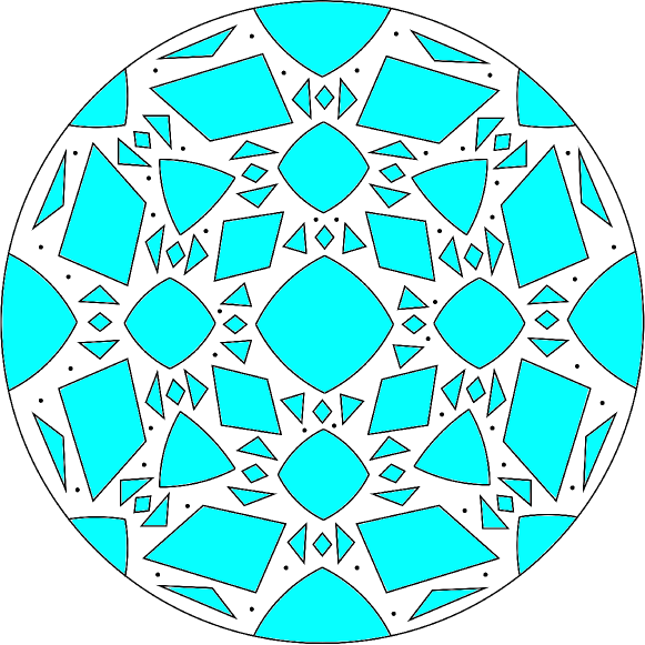
Figure 10: The angular diagram for a general dispersion relation $\,\epsilon({\bf p})\,$ (schematically, only a finite number of decreasing Stability Zones $\,\Omega^{*}_{\alpha}\,$ and special “chaotic” directions is shown).

Let us also note that on the boundaries of the Zones $\,\Omega^{*}_{\alpha}\,$ we have open trajectories of the system (1.1) having a regular form, shown at Fig. 1, which in this case are not stable with respect to all small rotations of $\,{\bf B}\,$, as well as energy level variations.

It is not difficult to see that the angular diagram of a Fermi surface, determined by one dispersion relation $\,\epsilon({\bf p})=\epsilon_{F}\,$, can be “nested” in the diagram of the total dispersion relation, so that the Stability Zones, defined for a fixed Fermi surface, represent subsets of a part of the Zones $\,\Omega^{*}_{\alpha}\,$. For Fermi surfaces defined by several dispersion relations, in general, such a natural embedding can be absent. It should be noted here that the latter situation arises actually only for sufficiently complex Fermi surfaces containing several complex components.

The complement to the set $\,\left\{\cup\,\overline{\Omega^{*}_{\alpha}}\right\}\,$ on the sphere $\,\mathbb{S}^{2}\,$ forms a rather complex set (of Cantor type) and represents the directions of $\,{\bf B}\,$ corresponding to the appearance of chaotic open trajectories at one energy level

$$\epsilon_{0}({\bf B}/B)\,\,\,=\,\,\,\tilde{\epsilon}_{1}({\bf B}/B)\,\,\,=\,\,\,\tilde{\epsilon}_{2}({\bf B}/B)$$

According to the conjecture of S.P. Novikov (see [36]), this set has measure zero and the Hausdorff dimension strictly less than 2 on the unit sphere. We can note here that the structure of the set of such special directions and the properties of chaotic trajectories are actively investigated at the present time (see, e.g. [16, 18, 33, 51, 52, 53, 55, 5, 6, 8, 56, 9, 19, 10, 46, 47, 20, 21, 2, 3, 11]).

In conclusion of this chapter, it can be noted that although angular diagrams of conductivity for the complete dispersion relation are not yet observed in the experiment, it is possible that they will still be observed in the measurement of (photoinduced) conductivity in semiconductors in extremely strong magnetic fields (see [17]).

3 Chaotic trajectories and two-dimensional electron systems.

In this chapter we will consider the trajectories of the system (1.1), which have chaotic properties. We will start with a simpler example, constructed by S.P. Tsarev (private communication, 1992-1993). The general idea of constructing chaotic trajectories, suggested by Tsarev, can be expressed by the following scheme:

Consider a family of identical integral (horizontal) planes connected by identical cylinders, as shown at Fig. 11. Let us assume that the centers of all the bases of the cylinders shown at Fig. 11 lie in one (for simplicity, vertical) plane intersecting the horizontal planes in some direction $\,\hat{\alpha}$. We also assume that the constructed cylinders are repeated periodically, so that the constructed surface is periodic with some periods $\,{\bf a}_{1}$, $\,{\bf a}_{2}$, lying in the horizontal plane, and also a vertical period $\,{\bf a}_{3}$. It is not difficult to see that the constructed surface can be regarded as a periodic Fermi surface, and we must divide all the integral planes (even and odd), and the cylinders ($C_{1}$ and $C_{2}$) into two different classes. Let us consider a horizontal magnetic field $\,{\bf B}$, orthogonal to the direction $\,\hat{\alpha}$, and the trajectories of the system (1.1) corresponding to this direction. The trajectories of the system (1.1) can be considered as trajectories on integral planes (of two different types), sometimes jumping from one plane to another. Under the above conditions, it is not difficult to see that any trajectory that jumps from a plane to an adjacent plane inevitably jumps to the next plane and continues in the same direction as on the original plane (Fig. 11). It is easy to see here that all the (non-singular) trajectories of the system (1.1) have an asymptotic direction in the $\,{\bf p}$ - space defined by the relations between the effective radius of the cylinders and the periods $\,{\bf a}_{1}$, $\,{\bf a}_{2}$, $\,{\bf a}_{3}$. At the same time, for any irrational direction $\,\hat{\alpha}\,$ (with respect to the given crystal lattice), no regular trajectory of (1.1) can lie in a straight line of finite width in the corresponding plane, orthogonal to $\,{\bf B}$.

Figure 11: The Brillouin zone and the behavior of the trajectories of the system (1.1) for a Fermi surface carrying chaotic trajectories of Tsarev type.

It is easy to see, that in the above construction each regular trajectory of the system (1.1) sweeps out half the surface of genus 3 and, in this sense, has a chaotic behavior on the Fermi surface. In the extended $\,{\bf p}$ - space, however, the trajectories of Tsarev are more like the trajectories described in the previous chapter, having asymptotic directions in the plane orthogonal to $\,{\bf B}$. As was shown in [16], the last property is actually observed for all chaotic trajectories arising for directions of $\,{\bf B}\,$ of irrationality 2 (the plane orthogonal to $\,{\bf B}$ contains a reciprocal lattice vector). As in the case of stable open trajectories, the contribution of Tsarev’s chaotic trajectories to magnetoconductivity has a more complex analytic behavior than that given by the formula (1.3), but has similar geometric properties. In particular, here also the general formula (2.1) takes place with a proper choice of the coordinate system.

More complex examples of chaotic trajectories of the system (1.1) were first constructed by I.A. Dynnikov in the work [16]. The Dynnikov trajectories arise for directions of $\,{\bf B}\,$ of maximal irrationality and have complex chaotic behavior both on the Fermi surface and in the extended $\,{\bf p}$ - space. As a rule, the Dynnikov trajectories everywhere densely sweep components of genus 3 (or more) with contractible holes in the Brillouin zone, having an obvious chaotic behavior on these components. In the extended $\,{\bf p}$ - space, the behavior of such trajectories in planes orthogonal to $\,{\bf B}$, resembles diffusional motion to some extent, although, of course, it is not diffusion in the strict sense of the word (Fig. 12). In general, the behavior of trajectories of this type on the Fermi surface and in the extended $\,{\bf p}$ - space represents an important example of an emergence of classical chaos in the condensed matter physics.

Figure 12: Dynnikov chaotic trajectory in a plane orthogonal to $\,{\bf B}$.

The behavior of the magnetoconductivity (and other transport phenomena) in strong magnetic fields in the presence of chaotic trajectories of Dynnikov type on the Fermi surface has the most complicated form. The most interesting phenomenon arising in this case is the suppression of the conductivity along the direction of the magnetic field in the limit $\,\omega_{B}\tau\rightarrow\infty\,$ ([33]). Thus, because the chaotic trajectory sweeps out a part of the Fermi surface, which is invariant under the transformation $\,{\bf p}\,\rightarrow\,-{\bf p}\,$, the contribution of this part to the longitudinal conductivity disappears in the above limit. In this situation, the longitudinal conductivity is created only by the remaining part of the Fermi surface filled with closed trajectories of the system (1.1). As a consequence of this fact, the longitudinal conductivity must have sharp minima for the directions of $\,{\bf B}$ corresponding to the appearance of such trajectories on the Fermi surface.

Another interesting circumstance arising in the description of transport phenomena in the presence of Dynnikov-type trajectories on the Fermi surface is the appearance of fractional powers of the parameter $\,\omega_{B}\tau\,$ in the asymptotic behavior of the components of the tensor $\,\sigma^{ik}(B)\,$ as $\,\omega_{B}\tau\rightarrow\infty\,$ ([33, 41]). Let us note here that the first indication of this circumstance in [33] was actually based on some additional property of the trajectories (self-similarity) constructed in [16]. It must be said that this property is not, generally speaking, common for trajectories of the Dynnikov type. Nevertheless, as can be shown (see [41]), the appearance of such powers is in fact a more general fact and is associated with important characteristics (the Zorich - Kontsevich - Forni indices) of dynamical systems on surfaces. The Zorich - Kontsevich - Forni indices play an important role in describing the behavior of the trajectories of dynamical systems and can be determined for a fairly wide class of dynamical systems and foliations on surfaces (see [51, 52, 53, 54, 55, 56]). Let us also note here that for the dynamical system (1.1) the existence of the Zorich - Kontsevich - Forni indices, strictly speaking, requires additional justification and does not follow automatically from the general theory based on certain generic requirements. As an example of such a justification, we can indicate the work [2], in which the construction and investigation of Dynnikov type trajectories was carried out, and the existence of the indicated indices for the Fermi surface of a rather general form was established.

We give here a general description of the Zorich - Kontsevich - Forni indices defined in the general case for foliations generated by closed 1-forms on compact surfaces $\,M^{2}_{g}$. We will follow here the work [55], where for “almost all” foliations of this type the following properties were indicated:

For a foliation generated by a closed 1-form on a surface of genus $\,g$, we consider a layer (level line) in general position and fix an initial point $\,P_{0}\,$ on it. On the same layer, we fix another point $\,P_{1}\,$, in which this layer approaches close to $\,P_{0}\,$ after passing a sufficiently large path along the surface $\,M^{2}_{g}$. We join the points $\,P_{0}\,$ and $\,P_{1}\,$ by a short segment and define a closed cycle on the surface $\,M^{2}_{g}$. Let us denote the homology class of the resulting cycle by $\,c_{P_{0}}(l)\,$, where $\,l\,$ represents the length of the corresponding section of the layer in some metric. Then:

There is a flag of subspaces

$$V_{1}\,\,\subset\,\,V_{2}\,\,\subseteq\,\,\dots\,\,\subseteq\,\,V_{g}\,\,\subseteq\,\,V\,\,\subset\,\,H_{1}(M^{2}_{g};\mathbb{R})\,\,\,,$$

such that:

1) For any such layer $\,\gamma\,$ and any point $\,\,P_{0}\,\in\,\gamma\,\,$

$$\lim_{l\rightarrow\infty}\,\,{c_{P_{0}}(l)\over l}\,\,\,=\,\,\,c\,\,\,,$$

where the non-zero asymptotic cycle $\,\,c\,\in\,H_{1}(M^{2}_{g};\mathbb{R})\,\,$ is proportional to the Poincare cycle and generates the subspace $\,V_{1}\,$.

2) For any linear form $\,\,\phi\,\in\,Ann(V_{j})\,\subset\,H_{1}(M^{2}_{g};\mathbb{R})\,$, $\,\,\phi\notin\,Ann(V_{j+1})\,\,$

$$\limsup_{l\rightarrow\infty}\,\,{\log|\langle\phi,c_{P_{0}}(l)\rangle|\over\log l}\,\,\,=\,\,\,\nu_{j+1}\quad,\quad\quad j\,=\,1,\,\dots,\,g-1$$ (3.1)

3) For any $\,\,\phi\,\in\,Ann(V)\,\subset\,H_{1}(M^{2}_{g};\mathbb{R})\,$, $\,\,||\phi||\,=\,1\,\,$

$$|\langle\phi,c_{P_{0}}(l)\rangle|\,\,\leq\,\,const\,\,\,,$$

where the constant is determined only by foliation.

4) The subspace $\,\,V\,\subset\,H_{1}(M^{2}_{g};\mathbb{R})\,\,$ is Lagrangian in homology, where the symplectic structure is determined by the intersection form.

5) Convergence to all the above limits is uniform in $\,\gamma\,$ and $\,\,P_{0}\,\in\,\gamma\,$, i.e. depends only on $\,l\,$.

It can be seen that the above statements give extremely important information about the behavior of level lines of a foliation (or trajectories of a dynamical system) on the manifold $\,M^{2}_{g}$. It can also be shown that the properties described above also significantly affect the behavior of chaotic trajectories in the extended $\,{\bf p}$ - space under the condition that the Zorich - Kontsevich - Forni indices exist for the system (1.1) on the Fermi surface. Indeed, suppose that for some system (1.1) chaotic Dynnikov trajectories arise on a complex Fermi surface and fill a part of the Fermi surface bounded by closed singular trajectories. For greater rigorousness, we can use the procedure of gluing the corresponding holes in the $\,{\bf p}$ - space and define a new smooth Fermi surface carrying chaotic trajectories of the same global geometry as the system (1.1) (see [18]). We also put for simplicity (as is the case for the most realistic situations), that the corresponding carriers of chaotic trajectories have genus 3.

Under the condition that the Zorich - Kontsevich - Forni indices exist for the system under consideration, we can in this case speak of the presence of a flag of subspaces

$$V_{1}\,\,\subset\,\,V_{2}\,\,\subseteq\,\,V_{3}\,\,\subseteq\,\,V\,\,\subset\,\,H_{1}(M^{2}_{3};\mathbb{R})\,\,\,,$$

possessing the properties listed above.

We note that in the generic case we assume that $\,\,1\,>\,\nu_{2}\,>\,\nu_{3}\,>\,0\,$, $\,\,dim\,V_{2}\,=\,2\,$, $\,\,dim\,V_{3}\,=\,dim\,V\,=\,3\,$.

To describe the properties of the trajectories of the system (1.1) in the extended $\,{\bf p}$ - space which we need, let us now consider the map in homology

$$H_{1}(M^{2}_{g};\mathbb{R})\,\,\,\rightarrow\,\,\,H_{1}(\mathbb{T}^{3};\mathbb{R})\,\,\,,$$

induced by the embedding $\,\,M^{2}_{3}\,\subset\,\mathbb{T}^{3}\,$. It is not difficult to see that the images of all spaces $\,V_{j}\,$ must belong to a two-dimensional subspace defined by the plane orthogonal to $\,{\bf B}\,$. In addition, from the absence of a linear growth of the deviation from the point $\,P_{0}\,$ with increasing length of a trajectory in the plane orthogonal to $\,{\bf B}\,$ in examples of chaotic trajectories of Dynnikov type we get that the image of the asymptotic cycle $\,c\,$ is equal to zero under this mapping. The image of the subspace $\,V_{2}\,$ in the generic case is one-dimensional and determines the selected direction in the plane orthogonal to $\,{\bf B}\,$, along which the average deviation of the trajectory grows faster with its length $\,(\sim l^{\nu_{2}})\,$, than in the direction orthogonal to it. In the general case, we must also assume that the image of the space $\,V_{3}\,$ is two-dimensional and coincides with the plane orthogonal to $\,{\bf B}\,$. Considering the 1-forms $\,dp_{x}\,$ and $\,dp_{y}\,$ as a basis of 1-forms, subject to the above condition (2), we can in our situation choose the coordinate system $\,(x,y,z)\,$ in such a way that for some reference sequences of values $\,l\,$ we will have the relations

$$|\Delta p_{x}(l)|\,\,\,\simeq\,\,\,p_{F}\,\left({l\over p_{F}}\right)^{\nu_{2}}\quad,\quad\quad|\Delta p_{y}(l)|\,\,\,\simeq\,\,\,p_{F}\,\left({l\over p_{F}}\right)^{\nu_{3}}$$

for the deviations of the trajectory along the coordinates $\,p_{x}\,$ and $\,p_{y}\,$ when passing a part of the approximate cycles on the Fermi surface described above.

It can thus be seen that the existence of the Zorich - Kontsevich - Forni indices predetermines certain properties of “wandering” of electron trajectories in the extended $\,{\bf p}$ - space, and, consequently, in the coordinate space, according to the specifics of the electron motion in magnetic fields. In turn, as well as for closed or stable open trajectories, the geometric properties of chaotic trajectories have a decisive influence on the characteristics of electron transport phenomena in strong magnetic fields. In particular, we can expect here the manifestation of the Zorich - Kontsevich - Forni indices in the study of the magnetoconductivity in crystals in the limit $\,\omega_{B}\tau\rightarrow\infty\,$.

Indeed, as a more detailed analysis of the kinetic equations in this situation shows (see [41]), the existence of the Zorich - Kontsevich - Forni indices is manifested directly in the behavior of the components of the conductivity tensor in the plane, orthogonal to $\,{\bf B}$, and, in particular, leads to the following dependencies of the components $\,\sigma^{xx}\,$ and $\,\sigma^{yy}\,$ on the magnetic field:

$$\sigma^{xx}(B)\,\,\,\simeq\,\,\,{ne^{2}\tau\over m^{*}}\,\left(\omega_{B}\tau\right)^{2\nu_{3}-2}\quad,\quad\quad\sigma^{yy}(B)\,\,\,\simeq\,\,\,{ne^{2}\tau\over m^{*}}\,\left(\omega_{B}\tau\right)^{2\nu_{2}-2}$$

It should be noted here that the above relations do not in fact represent the principal term of any asymptotic expansion of the quantities $\,\sigma^{xx}(B)\,$ and $\,\sigma^{yy}(B)\,$ and define more likely some common “trend” in their behavior. Strictly speaking, it is also more correct here to write the relations

$$\limsup_{\omega_{B}\tau\rightarrow\infty}\,\,{\log\sigma^{xx}(B)\over\log\omega_{B}\tau}\,\,\,=\,\,\,2\nu_{3}\,-\,2\,\,\,,\quad\quad\limsup_{\omega_{B}\tau\rightarrow\infty}\,\,{\log\sigma^{yy}(B)\over\log\omega_{B}\tau}\,\,\,=\,\,\,2\nu_{2}\,-\,2$$

in the limit of strong magnetic fields. This trend, however, represents a very important general characteristic of the behavior of the quantities $\,\sigma^{xx}(B)\,$ and $\,\sigma^{yy}(B)\,$, since their exact dependence satisfies actually a number of important restrictions.

We note here, in addition, that the presence of the Zorich - Kontsevich - Forni indices for chaotic trajectories of Dynnikov type also allows us to write the following relation

$$\limsup_{\omega_{B}\tau\rightarrow\infty}\,\,{\log|\Delta s^{xy}(B)|\over\log\omega_{B}\tau}\,\,\,\,\,\leq\,\,\,\,\,\nu_{2}\,+\,\nu_{3}\,-\,2$$

for the contribution of such trajectories to the off-diagonal term of the symmetric part of the conductivity tensor in the plane orthogonal to $\,{\bf B}$, which can also serve as an estimate for the overall trend of the decrease of this quantity (see [41]).

We would now like to note that all the above relations have been obtained within the framework of the kinetic theory on the basis of a purely quasiclassical analysis of the evolution of electron states in crystalline conductors. At the same time, as is well known, electron transport phenomena in sufficiently strong magnetic fields also have observable quantum corrections caused by quantum phenomena in electron systems (see e.g. [1, 25, 32, 49]). Here we would like to note that for Dynnikov chaotic trajectories (unlike most other trajectories of other types) the most significant of the quantum effects is the phenomenon of magnetic breakdown that arises in sufficiently strong magnetic fields. The phenomenon of (intraband) magnetic breakdown here is closely related actually to the presence of saddle singular points inside carriers of chaotic trajectories and consists in the possibility of jumps from one section of the trajectory to another (at a fixed $\,p_{z}$) for a sufficiently close approach of such sections to each other (Fig. 13).

Figure 13: The phenomenon of magnetic breakdown on the Dynnikov chaotic trajectory in strong magnetic fields.

The jump probability for two given sections increases with increasing of $\,B\,$ and tends to $\,1/2\,$ in the limit $\,B\rightarrow\infty\,$. It is not difficult to see here that the mean time $\,\tau_{(1)}(B)\,$ of the electron motion between such jumps is a sufficiently rapidly decreasing function of $\,B\,$. The effect of magnetic breakdown becomes significant when $\,\tau_{(1)}(B)\,$ turns out to be of order of $\,\tau\,$, and the problem represents one of the possible models of quantum chaos in the limit $\,\tau_{(1)}(B)\,\ll\,\tau\,$. In the general case, the main effect of magnetic breakdown on transport phenomena in magnetic fields can be expressed by introducing the effective mean free time $\,\tau_{eff}(B)\,$, determined by the formula

$$\tau^{-1}_{eff}(B)\,\,\,=\,\,\,\tau^{-1}\,+\,\tau^{-1}_{(1)}(B)$$

As already noted, the phenomenon of magnetic breakdown represents a purely quantum phenomenon in the electron system. For a more detailed description of the quantum picture arising in the presence of chaotic trajectories on the Fermi surface, it is first of all necessary to consider the spectrum of the one-electron states near the Fermi energy in this situation. Here it is most convenient to start the analysis of the one-electron spectrum from a purely quasiclassical spectrum, i.e. from the spectrum, described by the “quantization” of quasiclassical orbits in the $\,{\bf p}$ - space. As we told already, the Dynnikov chaotic trajectories exist only on one energy level $\,\epsilon_{0}\,$ (see [15, 16, 18]), which should be close enough to the Fermi energy for the possibility of experimental observation of the regimes described above. At the energy levels $\,\epsilon<\epsilon_{0}\,$ all such trajectories break up into long closed trajectories of the electron type, and at the levels $\,\epsilon>\epsilon_{0}\,$ - into closed trajectories of the hole type. It can thus be seen that in the purely quasiclassical approximation (implying also the limit $\,\tau\rightarrow\infty$), we should expect the appearance of delocalized electron states only at the level $\,\epsilon=\epsilon_{0}\,$, while electron states near the level $\,\epsilon_{0}\,$ must be localized and determined by the quantization on the long closed trajectories.

In accordance with the rules of the quasiclassical quantization (see [1, 25, 32, 49], the closed trajectories of the system (1.1) for each $\,p_{z}\,$ should be selected according to the rule

$$S(\epsilon,p_{z})\,\,\,=\,\,\,{2\pi e\hbar B\over c}\,\left(n+{1\over 2}\right)\,\,\,,\quad n\gg 1\,\,\,,$$

where $\,S(\epsilon,p_{z})\,$ represents the area bounded by a closed trajectory in the plane orthogonal to $\,{\bf B}\,$ in the ${\bf p}$ - space.

It is easy to see that the areas of long closed trajectories $\,S(\epsilon,p_{z})\,$ tend to infinity as $\,\epsilon\rightarrow\epsilon_{0}\,$, which leads to a rapid decrease in the distance between electron levels in the same limit (Fig. 14). Such a behavior of the arising quasiclassical levels makes it possible to easily distinguish their contribution to a number of quantum corrections on the background of the contribution of electron levels arising on “short” closed trajectories of the system (1.1), the distance between which considerably exceeds the distance between levels arising on long closed trajectories of (1.1). Let us note here also that in studying the phenomena associated with the quantization of electron levels, usually the levels associated with the extremal trajectories on the Fermi surface, satisfying the condition $\,\partial S/\partial p_{z}\,=\,0\,\,\,,$ are revealed.

Figure 14: Quasiclassical electron levels near a special energy level carrying chaotic trajectories of the system (1.1).

In the absence of the magnetic breakdown, the level structure shown at Fig. 14, is destroyed by scattering on impurities under the condition $\,T\,\geq\,\tau\,$ near the level $\,\epsilon_{0}\,$. Scattering on impurities is associated with the electron motion in the coordinate space and “mixes” electron levels with different $\,p_{z}\,$, making the problem of determining of the new level structure essentially three-dimensional. It can be seen, however, that for a sufficiently large value of the magnetic field, we can have a much wider region near the value $\,\epsilon_{0}\,$, where the conditions $\,T\,\geq\,\tau_{(1)}(B)\,$ and $\,\tau_{(1)}(B)\,\ll\,\tau\,$ are fulfilled. In the corresponding region, the change in the structure of the electron levels will be completely determined by the phenomenon of the magnetic breakdown and will be described by the behavior of the levels of two-dimensional systems for fixed values of $\,p_{z}\,$. Systems of this type can be considered as one of the important models of quantum chaos, where a two-dimensional electron system has special quasiperiodic properties. The study of the structure of electron levels, as well as the transport properties of such systems, represents an important problem here both from the point of view of the mathematical theory of quantum chaos and from the point of view of the condensed matter physics.

As already noted, all the above regimes are observed for special directions of $\,{\bf B}\,$, corresponding to the appearance of chaotic trajectories of Dynnikov type on the Fermi surface. It must be said that for many of the real substances, such directions may in fact not be present on the angular diagram. In the general case, as was shown by I.A. Dynnikov (see [16, 18]), the Lebesgue measure of the corresponding directions on the angular diagram for generic Fermi surface is equal to zero. According to the conjecture of S.P. Novikov ([34, 35]), the fractal dimension of the set of such directions on the angular diagram for generic Fermi surface is strictly less than 1 (but may be larger for special Fermi surfaces). Nevertheless, for substances with a rather complex Fermi surface, it is quite possible to expect an experimental observation of the described regimes for specially selected directions of $\,{\bf B}\,$. In particular, the appearance of chaotic trajectories at levels arbitrarily close to the Fermi level should always be observed on the angular diagrams of type B described in the previous chapter. It should also be noted that stable open trajectories, corresponding to sufficiently small Stability Zones $\,\Omega_{\alpha}\,$, can also have a rather complex shape (Fig. 15) and have the features of both regular and chaotic behavior depending on the interval of the values of the parameter $\,\omega_{B}\tau\,$.

Figure 15: A stable open trajectory in the Zone $\,\Omega_{\alpha}\,$ of small sizes.

In conclusion of this chapter we consider briefly one more application of the Novikov problem to two-dimensional electron systems, which is actively studied in modern experiments. Namely, we consider the problem of a two-dimensional electron gas with a high mobility of carriers placed in the artificially created potential $\,V({\bf r})\,$. We note at once that at the present time there are many different methods of creating potentials of this type, many of them, in fact, are based on the use of superposition of certain periodic structures formed in the plane of the electron system. One of the most common methods, in particular, is the use of superposition of (one-dimensional) interference patterns of laser radiation, which causes the polarization of atoms forming the sample (see e.g. [48]).

Figure 16: Quasiperiodic potentials with three and four quasiperiods, obtained by superposition of three and four one-dimensional potentials with different directions and period values, respectively.

The Novikov problem in these systems arises in the description of electron transport phenomena in the presence of a sufficiently strong magnetic field $\,{\bf B}\,$, orthogonal to the sample plane. The quasiclassical consideration of the electron motion (see e.g. [23, 4]) allows one to use here the approximation of quasiclassical cyclotron orbits whose centers drift in the presence of the potential $\,V({\bf r})\,$ (Fig. 17). As can be shown, the drift of cyclotron orbit centers occurs along the level lines of the potential $\,V({\bf r})\,$ averaged over the corresponding cyclotron orbits. As in the case of normal metals, the main role here is played by electrons with energy close to the Fermi energy, so that for the electron motion one can also introduce a fixed cyclotron radius $\,r_{B}\,$ corresponding to the given problem. It is not difficult to see that the averaged potential $\,\bar{V}_{B}({\bf r})\,$ has then the same quasiperiodic properties as the potential $\,V({\bf r})\,$, and the description of the motion of orbits along the level lines of such a potential represents the Novikov problem with the corresponding number of quasiperiods.

Figure 17: The cyclotron orbit in the presence of a quasiperiodic potential $\,V({\bf r})\,$.

The great similarity between the two problems presented above makes it possible to transfer many results from the theory of the conductivity of normal metals to the theory of transport phenomena in the described two-dimensional systems (see e.g. [37]). We would like to note here that in the situation of two-dimensional systems, a much larger number of parameters of the system is controlled, which makes it possible to actually implement practically any of the interesting cases that arise in the investigation of the Novikov problem. In particular, two-dimensional electron systems can be a convenient experimental tool for studying chaotic regimes for specially selected parameters of such systems. It can also be noted here that by specifically choosing the parameters of the system, one can implement here both a purely quasiclassical case of chaotic behavior and a magnetic breakdown mode on chaotic trajectories. The latter circumstance is actually due to the fact that the semiclassical description here is also approximate, and here also jumps of cyclotron orbits between level lines of $\,\bar{V}_{B}({\bf r})\,$, close enough to each other, are possible (see [23]). As can be shown, different behavior modes (in the limit $\,\tau\rightarrow\infty$) are determined here by external parameters of the system. In general, it can be noted that the described two-dimensional electron systems can represent a very convenient experimental base for studying both regular regimes in magnetotransport phenomena and the models of classical and quantum chaos described above.

In conclusion, let us formulate a theorem that defines an important class of quasiperiodic functions on a plane with four quasiperiods whose level lines have properties analogous to the properties of stable open trajectories of the system (1.1) (see [45, 22]). We give here, in fact, only the main corollaries of the results obtained in [45, 22], a more detailed description of the resulting topological picture can be found in the papers [45, 22]. It can be recalled here that a quasiperiodic function on a plane with four quasiperiods $\,f\,$ is defined as the restriction to the plane of some 4-periodic function $\,F\,$ in four-dimensional space under a linear embedding $\,\mathbb{R}^{2}\subset\mathbb{R}^{4}\,$. According to [45, 22], the following assertion can be stated:

1) All non-singular open level lines of the corresponding functions $\,f\,$ in $\,\mathbb{R}^{2}\,$ lie in straight strips of finite width, passing through them;

2) The mean direction of all non-singular open level lines of the functions $\,f\,$ is given by the intersection of the corresponding plane $\,\mathbb{R}^{2}\,$ with some integral three-dimensional plane $\,\Gamma_{\alpha}(\Pi)\,$ in the space $\,\mathbb{R}^{4}\,$, which is locally constant in the space $\,G_{4,2}\,$.

It is not difficult to see that the statements formulated above correlate in a certain sense with the results obtained in the paper [50] for the case of quasiperiodic functions with three quasiperiods. It should also be noted that the proof of this theorem in the case of four quasiperiods requires, in fact, much greater effort.

References

- [1] A.A. Abrikosov., Fundamentals of the Theory of Metals., Elsevier Science & Technology, Oxford, United Kingdom, 1988.
- [2] A. Avila, P. Hubert, A. Skripchenko., Diffusion for chaotic plane sections of 3-periodic surfaces., Inventiones mathematicae, October 2016, Volume 206, Issue 1, pp 109–146.
- [3] A. Avila, P. Hubert, A. Skripchenko., On the Hausdorff dimension of the Rauzy gasket., Bulletin de la societe mathematique de France, 2016, 144 (3), pp. 539 - 568.
- [4] C. W. J. Beenakker, Guiding-center-drift resonance in a periodically modulated two-dimensional electron gas., Phys. Rev. Lett. 62, 2020 (1989).
- [5] R. De Leo., Existence and measure of ergodic leaves in Novikov’s problem on the semiclassical motion of an electron., Russian Math. Surveys 55:1 (2000), 166-168.
- [6] R. De Leo., Characterization of the set of “ergodic directions” in Novikov’s problem of quasi-electron orbits in normal metals., Russian Math. Surveys 58:5 (2003), 1042-1043.
- [7] R. De Leo., First-principles generation of stereographic maps for high-field magnetoresistance in normal metals: An application to Au and Ag., Physica B: Condensed Matter 362 (1-4) (2005), 62–75.
- [8] R. De Leo., Topology of plane sections of periodic polyhedra with an application to the Truncated Octahedron., Experimental Mathematics 15:1 (2006), 109-124.
- [9] R. De Leo, I.A. Dynnikov., An example of a fractal set of plane directions having chaotic intersections with a fixed 3-periodic surface., Russian Math. Surveys 62:5 (2007), 990-992.
- [10] R. De Leo, I.A. Dynnikov., Geometry of plane sections of the infinite regular skew polyhedron ., Geom. Dedicata 138:1 (2009), 51-67.
- [11] Roberto De Leo., A survey on quasiperiodic topology., arXiv:1711.01716
- [12] Yu.A. Dreizin, A.M. Dykhne., Anomalous Conductivity of Inhomogeneous Media in a Strong Magnetic Field., Journal of Experimental and Theoretical Physics, Vol. 36, No. 1 (1973), 127-136.
- [13] Yu.A. Dreizin, A.M. Dykhne., A qualitative theory of the effective conductivity of polycrystals., Journal of Experimental and Theoretical Physics, Vol. 57, No. 5 (1983), 1024-1026.
- [14] I.A. Dynnikov., Proof of S.P. Novikov’s conjecture for the case of small perturbations of rational magnetic fields., Russian Math. Surveys 47:3 (1992), 172-173.
- [15] I.A. Dynnikov., Proof of S.P. Novikov’s conjecture on the semiclassical motion of an electron., Math. Notes 53:5 (1993), 495-501.
- [16] I.A. Dynnikov., Semiclassical motion of the electron. A proof of the Novikov conjecture in general position and counterexamples., Solitons, geometry, and topology: on the crossroad, Amer. Math. Soc. Transl. Ser. 2, 179, Amer. Math. Soc., Providence, RI, 1997, 45-73.
- [17] I.A. Dynnikov, A.Ya. Maltsev., Topological characteristics of electronic spectra of single crystals., Journal of Experimental and Theoretical Physics 85:1 (1997), 205-208.
- [18] I.A. Dynnikov., The geometry of stability regions in Novikov’s problem on the semiclassical motion of an electron., Russian Math. Surveys 54:1 (1999), 21-59.
- [19] I.A. Dynnikov., Interval identification systems and plane sections of 3-periodic surfaces., Proceedings of the Steklov Institute of Mathematics 263:1 (2008), 65-77.
- [20] I. Dynnikov, A. Skripchenko., On typical leaves of a measured foliated 2-complex of thin type., Topology, Geometry, Integrable Systems, and Mathematical Physics: Novikov’s Seminar 2012-2014, Advances in the Mathematical Sciences., Amer. Math. Soc. Transl. Ser. 2, 234, eds. V.M. Buchstaber, B.A. Dubrovin, I.M. Krichever, Amer. Math. Soc., Providence, RI, 2014, 173-200, arXiv: 1309.4884
- [21] I. Dynnikov, A. Skripchenko., Symmetric band complexes of thin type and chaotic sections which are not actually chaotic., Trans. Moscow Math. Soc., Vol. 76, no. 2, 2015, 287-308.
- [22] I.A. Dynnikov, S.P. Novikov., Topology of quasi-periodic functions on the plane., Russian Math. Surveys 60:1 (2005), 1-26.
- [23] H.A. Fertig., Semiclassical description of a two-dimensional electron in a strong magnetic field and an external potential., Phys. Rev. B 38 (1988), 996-1015.
- [24] M.I. Kaganov, V.G. Peschansky., Galvano-magnetic phenomena today and forty years ago., Physics Reports 372 (2002), 445-487.
- [25] C. Kittel., Quantum Theory of Solids., Wiley, 1963.
- [26] I.M.Lifshitz, M.Ya.Azbel, M.I.Kaganov. The Theory of Galvanomagnetic Effects in Metals., Sov. Phys. JETP 4:1 (1957), 41.
- [27] I.M. Lifshitz, V.G. Peschansky., Galvanomagnetic characteristics of metals with open Fermi surfaces., Sov. Phys. JETP 8:5 (1959), 875.
- [28] I.M. Lifshitz, V.G. Peschansky., Galvanomagnetic characteristics of metals with open Fermi surfaces. II., Sov. Phys. JETP 11:1 (1960), 137.
- [29] I.M. Lifshitz, M.I. Kaganov., Some problems of the electron theory of metals I. Classical and quantum mechanics of electrons in metals., Sov. Phys. Usp. 2:6 (1960), 831-835.
- [30] I.M. Lifshitz, M.I. Kaganov., Some problems of the electron theory of metals II. Statistical mechanics and thermodynamics of electrons in metals., Sov. Phys. Usp. 5:6 (1963), 878-907.
- [31] I.M. Lifshitz, M.I. Kaganov., Some problems of the electron theory of metals III. Kinetic properties of electrons in metals., Sov. Phys. Usp. 8:6 (1966), 805-851.
- [32] I.M. Lifshitz, M.Ya. Azbel, M.I. Kaganov., Electron Theory of Metals. Moscow, Nauka, 1971. Translated: New York: Consultants Bureau, 1973.
- [33] A.Y. Maltsev., Anomalous behavior of the electrical conductivity tensor in strong magnetic fields., Journal of Experimental and Theoretical Physics 85 (5) (1997), 934-942.
- [34] A.Ya. Maltsev, S.P. Novikov., Quasiperiodic functions and Dynamical Systems in Quantum Solid State Physics., Bulletin of Braz. Math. Society, New Series 34:1 (2003), 171-210.
- [35] A.Ya. Maltsev, S.P. Novikov., Dynamical Systems, Topology and Conductivity in Normal Metals in strong magnetic fields., Journal of Statistical Physics 115:(1-2) (2004), 31-46.
- [36] A.Ya. Maltsev, S.P. Novikov., Dynamical Systems, Topology and Conductivity in Normal Metals., arXiv:cond-mat/0304471
- [37] A.Ya. Maltsev., Quasiperiodic functions theory and the superlattice potentials for a two-dimensional electron gas., Journal of Mathematical Physics 45:3 (2004), 1128-1149.
- [38] A.Ya. Maltsev., On the Analytical Properties of the Magneto-Conductivity in the Case of Presence of Stable Open Electron Trajectories on a Complex Fermi Surface., Journal of Experimental and Theoretical Physics 124 (5) (2017), 805-831.
- [39] A.Ya. Maltsev., Oscillation phenomena and experimental determination of exact mathematical stability zones for magneto-conductivity in metals having complicated Fermi surfaces., Journal of Experimental and Theoretical Physics 125:5 (2017), 896-905.
- [40] A.Ya. Maltsev., The second boundaries of Stability Zones and the angular diagrams of conductivity for metals having complicated Fermi surfaces., Journal of Experimental and Theoretical Physics 127:6 (2018), 1087-1111., arXiv:1804.10762
- [41] A.Ya. Maltsev, S.P. Novikov., The theory of closed 1-forms, levels of quasiperiodic functions and transport phenomena in electron systems., arXiv:1805.05210
- [42] S.P. Novikov., The Hamiltonian formalism and a many-valued analogue of Morse theory., Russian Math. Surveys 37 (5) (1982), 1-56.
- [43] S.P. Novikov, A.Y. Maltsev., Topological quantum characteristics observed in the investigation of the conductivity in normal metals., JETP Letters 63 (10) (1996), 855-860.
- [44] S.P. Novikov, A.Y. Maltsev., Topological phenomena in normal metals., Physics-Uspekhi 41:3 (1998), 231-239.
- [45] S.P. Novikov., Levels of quasiperiodic functions on a plane, and Hamiltonian systems., Russian Math. Surveys 54 (5) (1999), 1031-1032.
- [46] A. Skripchenko., Symmetric interval identification systems of order three., Discrete Contin. Dyn. Sys. 32:2 (2012), 643-656.
- [47] A. Skripchenko., On connectedness of chaotic sections of some 3-periodic surfaces., Ann. Glob. Anal. Geom. 43 (2013), 253-271.
- [48] D.Weiss, K.v. Klitzing, K. Ploog, and G. Weimann, Magnetoresistance oscillations in a two-dimensional electron gas induced by a submicrometer periodic potential., Europhys. Lett., 8 (2), 179 (1989).
- [49] J.M. Ziman., Principles of the Theory of Solids., Cambridge University Press 1972.
- [50] A.V. Zorich., A problem of Novikov on the semiclassical motion of an electron in a uniform almost rational magnetic field., Russian Math. Surveys 39 (5) (1984), 287-288.
- [51] A.V. Zorich., Asymptotic Flag of an Orientable Measured Foliation on a Surface., Proc. “Geometric Study of Foliations”., (Tokyo, November 1993), ed. T.Mizutani et al. Singapore: World Scientific Pb. Co., 479-498 (1994).
- [52] A.V. Zorich., Finite Gauss measure on the space of interval exchange transformations. Lyapunov exponents., Annales de l’Institut Fourier 46:2, (1996), 325-370.
- [53] Anton Zorich., On hyperplane sections of periodic surfaces., Solitons, Geometry, and Topology: On the Crossroad, V. M. Buchstaber and S. P. Novikov (eds.), Translations of the AMS, Ser. 2, vol. 179, AMS, Providence, RI (1997), 173-189.
- [54] Anton Zorich., Deviation for interval exchange transformations., Ergodic Theory and Dynamical Systems 17, (1997), 1477-1499.
- [55] Anton Zorich., How do the leaves of closed 1-form wind around a surface., “Pseudoperiodic Topology”, V.I.Arnold, M.Kontsevich, A.Zorich (eds.), Translations of the AMS, Ser. 2, vol. 197, AMS, Providence, RI, 1999, 135-178.
- [56] Anton Zorich., Flat surfaces., in collect. “Frontiers in Number Theory, Physics and Geometry. Vol. 1: On random matrices, zeta functions and dynamical systems”; Ecole de physique des Houches, France, March 9-21 2003, P. Cartier; B. Julia; P. Moussa; P. Vanhove (Editors), Springer-Verlag, Berlin, 2006, 439-586.