Virtual social science

Abstract

Can we describe social systems quantitatively and predictively, when we know all the actions, interactions, and states of individuals? We interpret human societies as co-evolutionary systems of individuals and their interactions. Based on unique data of a society of computer game players, where all actions and interactions between all players are known, we show that this might indeed be possible. Within this framework we address a number of sociological classics, including formation of social networks, strength of relations, group formation, hierarchical organization, aggression management, gender differences, mobility, and wealth-inequality. We discover behavioral and organizational patterns of the homo sapiens and its society that were not visible with traditional methodology from the social sciences.

1 Introduction

In the first years of the nineteenth century Auguste Comte suggested to copy what had been done in physics at this point in time: to establish a natural and experimental science of social systems. He suggested to call this hopeless endeavor sociophysics. No-one followed him. He died poor and alone, without any acknowledgement of this vision of his. Some remember him today as the inventor of the term sociology. Of course, his vision was bound to fail. There was no way of understanding what the rules of interactions between the components of societies were. Even had he known the interpersonal interaction laws, he would have failed. He would not yet have had a way to aggregate information of many interactors to levels that could have been interpreted in any meaningful way. Statistical mechanics was not invented yet, nor was the computer; Gauss was barely born. Had he overcome all these difficulties, he would have most likely failed because he did not have a way to know what non-linearity can do to the predictability of dynamical systems. He had to fail.

Now, more than 200 years later, we try it again: to transform the social science as we know it today, into an experimental physical science: fully quantitative, predictive, and experimentally testable. A science that is based on the elementary interactions between humans, and between them and their environment. Immediately criticism from the traditional representatives of the social sciences and humanities arises: (i) humans have a free will, their actions and interactions can not be predicted; (ii) societies have way too complicated interactions, which will never be quantifiable, and (iii) data on actions and interactions on a society-wide level does not exist.

In the 21st century we do not have to accept these arguments. None of them states a fundamental reason, why a new attempt would have to fail. In response to the free will argument (i), we can argue that atoms have even more “free will” than humans do, and that on a quantum mechanics level the situation is even worse: not only could an atom decay spontaneously, not even its position and momentum can be known simultaneously. How should we ever be able to predict properties of matter that is composed of such volatile things? But we can. A counter argument to statement (ii), that human interactions are too complicated to be quantified, is found in the very existence and availability of exactly this kind of data, together with the computer power to process it. We might be able to record a large fraction of all interactions soon, given that we are not stopping the current trends in digitation. The same holds true for argument (iii), that there is a lack of data on social actions and interactions. The world has changed.

This does not mean that those who try to realize the vision of Comte again will be successful. In this lecture I will show that in fact, we are getting to the point, where we will be able to record every single interaction in a social system, meaning that we have records about all interactions, at all times, and between all individuals. I will show a special example where we have exactly this situation: a dataset of a human society of players “living” in a massive multiplayer online game, where all information about actions, interactions and properties of all avatars is available. The game is called Pardus, and was developed, programmed, and maintained by my former students and collaborators Michael Szell and Werner Payer. In this game, which attracted almost half a million players since 2004, avatars act out an open-ended “second life”, over large periods of time—often over years. All actions and interactions, all properties and characteristics of all players are recorded, at every point in time.

We have studied this human society in the past years. In this lecture notes, I summarize some of the work that was done together with Michael Szell, Peter Klimek, Benedikt Fuchs, Renaud Lambiotte, Vito Latora, Roberta Sinatra, Didier Sornette, Olesya Mryglod, Yurko Holovatch, Bernat Corominas-Murtra, Maximilian Sadilek, and others. The original works are found in [1, 2, 3, 4, 5, 6, 7, 8, 9, 10, 11, 12, 13, 14, 15].

1.1 What is social science?

Social science is the science of social interactions and their implications for society. Traditionally, social science has neither been very quantitative or predictive, nor does it produce experimentally testable predictions. It is largely qualitative and descriptive. Until recently, there has been a tremendous shortage of data that are both, time-resolved (longitudinal) and multidimensional. As stated, the situation is changing fast with the tendency of homo sapiens to leave electronic fingerprints in practically all dimensions of life. The century-old data problem of the social sciences is rapidly disappearing. Another fundamental problem in the social sciences is the lack of reproducibility and repeatability. On many occasions, an event takes place once in history, and no repeats are possible.

As in biology, social processes are hard to understand mathematically because they are evolutionary, path-dependent, out-of-equilibrium, and context-dependent. They are high-dimensional and involve interactions on multiple levels and scales. The methodological tools used by traditional social scientists, which rarely extend much beyond linear regression models, and basic Gaussian statistics, are not powerful enough to address these issues appropriately. However, two important innovations have been developed within the social sciences that play a crucial role in the theory of complex systems:

Multilayer interaction networks. In social systems, interactions between individuals and institutions, happen simultaneously on more or less the same strength scale on a multitude of superimposed interaction networks. Social scientists, in particular sociologists, have recognized the importance of social networks, starting in the 1970s [16, 17].

Game theory. Another contribution is game theory, a concept that allows us to determine the outcome of rational interactions between agents trying to optimize their payoff or utility [18]. Each agent is aware of the fact that the other agent is rational and that he/she also knows that the other agent is rational. Before computers arrived on the scene, game theory was one of the few methods of dealing with complex systems (in equilibrium). Game theory can easily be transferred to dynamical situations, and it was believed for a long time that iterative game-theoretic interactions were a way of understanding the origin of cooperation in societies. This view is now severely challenged by the discovery of so-called zero-determinant games [19]. Game theory was first developed and used in economics, but later penetrated other fields of the social, behavioural, and life sciences.

1.1.1 Social systems are continuously restructuring networks

Social systems can be thought of as time-varying multilayer networks. Nodes are individuals or institutions; links are interactions of different type. Interactions change over time. The types of link can be friendship, family ties, processes of good exchange, payments, trust, communication, enmity, and so on. Every type of link is represented by a separate network layer, see e.g. Fig. 1. Individuals interact through a superposition of these different interaction types (multilayer network), which happen simultaneously, and are often of the same order of magnitude in “strength”. Often, networks at one level interact with networks at other levels. Networks that characterize social systems show a rich spectrum of growth patterns and a high level of plasticity. This plasticity of networks arises from restructuring processes through link creation, re-linking, and link removal. Understanding and describing the underlying restructuring dynamics can be challenging. However, there are a few typical and recurring dynamical patterns that allow us to make scientific progress.

Individuals are represented by “states”, a set of characteristics that describe their wealth, gender, education level, political opinion, age, and so on. Some of these states change dynamically over time. States typically have an influence on the linking dynamics of their corresponding node. If that is the case, a tight connection exists between network structure and node states. The joint dynamics of network re-structuring and changes of states by individuals is a classic example of co-evolution.

1.2 Social systems are complex systems

If social systems are complex systems—what are complex systems? We follow the definition of complex systems given in [20]: Complex systems are co-evolving multilayer networks. This statement summarizes ten facts about complex systems:

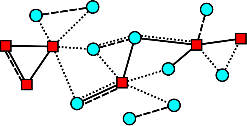
Figure 1: Schematic representation of a multilayer network. Here nodes are characterized by a two-dimensional state vector. The first component is given by colors (red, blue), the second by shapes (circles, squares). Nodes interact through three types of interaction that are represented by (full, broken, and dotted) lines. The system is complex if states simultaneously change as a function of the interaction network, and at the same time, if interactions change as a function of the states, see Eqs. (1). It is a co-evolving system, where states and interactions update each other, similar to what an algorithm is doing.

1. Complex systems are composed of multiple elements, labelled by latin indices, $i$.

2. These elements interact with each other through one or more interaction type, labelled by greek indices, $\alpha$. Interactions between elements are specific, not everyone interacts with all the others. To keep track of which elements interact we use networks. Interactions are represented as links, the interacting elements are nodes. Every interaction type can be seen as one network layer in a multilayer network, see Fig. 1. A multilayer network is a collection of networks linking the same set of nodes. If these networks evolve independently, multilayer networks are superpositions of networks. However, there are often interactions between interaction layers.

3. Interactions change over time. We use the following notation to keep track of interactions in the system. The strength of an interaction of type $\alpha$ between two elements $i$ and $j$ at time $t$ is denoted by,

   $$M_{ij}^{\alpha}(t)\quad{\rm interaction}\ {\rm strength}\quad.$$

   Interactions can be physical, financial, emotional, economical, hostile, or symbolic, to just mention a few. Most interactions are mediated by an exchange process of some sort between nodes. In that sense, interaction strength is often related to the quantity of “things” or units exchanged (money for financial interactions, love letters for emotional interactions, bullets for hostile interactions, bottles of wine for positive social interactions, and so on). Interactions can be deterministic or stochastic.

4. Elements are characterized by states. States can be scalar; if an element has various independent states, it will be described by a state vector, or a state tensor. States also evolve over time. We denote the state vectors by,

   $$\sigma_{i}(t)\quad{\rm\ state\ vector}\quad.$$

   States can be the education level, gender, political believe, wealth, aggression level of a person, or the capitalization, and risk aversion levels of a bank. State changes can be deterministic or stochastic. Changes can be the result of the endogenous dynamics in the multilayer network, or of external driving.

5. States and interactions are often not independent but evolve together by mutually influencing each other; states and interactions co-evolve. The way in which states and interactions are coupled can be deterministic or stochastic.

6. The dynamics of co-evolving multilayer networks is usually non-linear.

7. Complex systems are context-dependent. Multilayer networks provide that context. To be more precise, for any dynamic process happening on a given network layer, the other layers represent the “context” in the sense that they provide the only other ways in which elements in the initial layer can be influenced. Multilayer networks sometimes allow complex systems to be interpreted as “closed systems”. They can be externally driven. Then they are dissipative and non-Hamiltonian.

8. Complex systems are algorithmic, they behave rather like an algorithm than a system that is described by a set of differential equations. The algorithmic nature is a direct consequence of the discrete interactions between interaction networks and states.

9. Complex systems are path-dependent, and therefore often non-ergodic. Given that the network dynamics (the dynamics of links) is sufficiently slow, the networks in the various layers can be seen as a “memory” that stores the recent past of the system.

10. Complex systems often have memory. Information about the past can be stored in nodes if they have explicit memory, or in the network structure in the various layers.

In the following, we assume that a co-evolving multilayer network structure is the fundamental dynamical backbone of social systems. A snapshot of a co-evolving multilayer network is shown in Fig. 1. Nodes are given by a state vector with two components, colour (blue, red) and shape (circles and boxes). Nodes interact through three types of interaction (full, broken, and dotted lines). The system is a complex system if states change as a function (deterministic or stochastic) of the interaction network and, simultaneously, interactions (the networks) change as a function of the states. The shown multilayer network could represent a social network of individuals with certain time-dependent properties. Think of wealth represented by shape (rich=circle, poor=square), and gender (blue=male, red=female), and the different different link-types represent communication, trade, and friendship. While the state of wealth can change as a function of the trading links, gender will not change because of trading links, but might because of friendship links. Changes in wealth will have a positive influence on the creation of future trading links, and maybe a negative effect on friendship links.

1.2.1 What is co-evolution?

Interactions can change the states of elements. The interaction partners of a node in a (multilayer) network can be seen as the local “environment” of that node. The environment often determines the future state of the node. In social systems, interactions do change over time. For example, people establish new friendships or economic relations, countries terminate diplomatic relations. The state of nodes determines (fully or in part) the future state of the links, whether it exists in the future or not, and if it exists, the strength and the direction that it will have. The essence of co-evolution is expressed in the statement: The state of the network (topology and weights) determines the future states of the nodes. The state of the nodes determines the future states of the links of the network.

Formally, co-evolving multilayer networks can be written as

$$\frac{d}{dt}\sigma_{i}(t) \sim F\left(M_{ij}^{\alpha}(t),\sigma_{j}(t)\right)$$

$${\rm and}$$

$$\frac{d}{dt}M_{ij}^{\alpha}(t) \sim G\left(M_{ij}^{\beta}(t),\sigma_{j}(t)\right)\quad.$$ (1)

Here, the derivatives indicate “change within the next time step”, and are not continuous derivatives. The first equation means that the states of element $i$ change as a function, $F$, that depends on the present states of $\sigma_{i}$, and the present multilayer network states, $M_{ij}^{\alpha}(t)$. The function (or functional), $F$, can be deterministic or stochastic and contains all summations over all greek indices and over $j$. The first equation depicts the analytical nature of physics that characterized the past 300 years of science. Once one specifies $F$, and the initial conditions, say, $\sigma_{i}(t=0)$, the solution of the equation provides us with the trajectories of the elements of the system. In physics the interaction matrix, $M_{ij}^{\alpha}(t)$, could represent the four forces. Usually it only involves a single interaction type $\alpha$, that is static, fully connected, and interaction strength only depends on the relative distance between $i$ and $j$. Typically, systems that can be described with the first equation alone are not complex systems, however complicated they may be.

The second equation specifies how the interactions evolve over time as a function $G$ that depends on the same inputs, states and interaction networks. $G$ can be a deterministic or stochastic function or functional. Now, interactions evolve in time. In physics this is very rarely the case. The combination of both equations makes the system co-evolving and complex. Co-evolving systems of this type are, in general, no longer analytically solvable. One cannot solve these systems using the rationale of physics because the environment—or the boundary conditions—specified by $M$, change as the system evolves. Equations (1) are not useful until the functions $G$ and $F$ are well specified. The science of complex systems often tries to identify these functions for a concrete system at hand. Often this is done in an algorithmic way, meaning that $F$ and $G$ can be given as “update rules”.

More and more data sets containing full information about an entire system are becoming available, meaning that all state changes and all interactions between the elements are recorded. It is becoming technically and computationally possible to monitor cell-phone communications on a national scale [21], to track all airplanes in motion, or to track all legal financial transactions on the planet. Longitudinal data about states and interactions can be used to visualize Eqs. (1); all the necessary components are in the data at any point in time: the interaction networks, $M_{ij}^{\alpha}$, the states of the elements, $\sigma_{i}$, and all the changes $\frac{d}{dt}\sigma_{i}$ and $\frac{d}{dt}M_{ij}^{\alpha}$. Even though Eqs. (1) might not be analytically solvable, it is becoming possible for more and more situations to “watch” them.

The structure of Eqs. (1) is not the most general. One generalization is to endow multilayer networks with a second greek index, $M_{ij}^{\alpha\beta}$, that captures cross-layer interactions between elements [22]. It is conceivable that elements and interactions are embedded in space and time; indices labelling the elements and interactions could carry such additional information, $i(x,t,...)$ or $\{ij\}^{\alpha\beta}(x,t,...)$. One can introduce memory to the elements and interactions. We will make use of these generalizations in the following, where we use complete information on all the actions and interactions of ten thousands of players engaged in a massive multiplayer online game, with their millions of interactions and state-changes.

2 A virtual society

2.1 The universe: the Pardus game

Our habitat is Pardus (http://www.pardus.at), a browser-based MMOG in a science-fiction setting. There are about 480,000 registered Pardus players, about 16,000 active players on a given day, the game is online since Sep 2004, and is free of charge. MMOGs are characterized by a substantial number of users playing together in the same virtual environment connected by an internet browser [23, 24]. In Pardus every player owns one account with one single character or avatar. This avatar is a pilot owning a spacecraft with a certain cargo capacity, moving around in a virtual universe to produce and trade commodities and products, socialize, engage in social activities, wage wars, engage in administration, and much more. An important component of Pardus is that the actions and interactions of players are strongly driven by social factors such as friendship, cooperation, and competition. There is no explicit goal in Pardus, nor are there forbidden moves (with a few exceptions concerning decent behavior). Pardus is a virtual world with a gameplay based on socializing and role-playing, with massive interactions between players’ avatars, and with interactions with a non-player environment. Players simultaneously engage in three forms of “life”:

Economic life. They produce, distribute and trade goods and services, and make profit from economic activity. They spend money on goods and services, such as new space ships, equipment, and consumables. Status symbols play a big role in the purchase and consumption of goods. Social life. Players communicate and share information to organize in social structures and collective actions, be it social, political, legal, hostile, or economical. Often actions are driven by the wish to accumulate social status through one of many forms of earning recognition. Exploratory life. Players explore their universe. They produced maps of the universe and it resources, classified its game-specific fauna. Some even have engaged in research on the “physical nature” of the game.

While playing, players form groups of different sizes and structures. These include political parties, special interest groups, criminal gangs, cartels, banks, courts, self-defence groups, or armies. They also organize in clubs that are called alliances.

Daily database backups are recorded, and are available for more than a decade, starting from Sept 2005. These backups contain longitudinal information of the actions and properties (states) of the avatars, as well as all the interactions between them, and between them and the environment.

2.1.1 The census of avatars

Age and nationality. In a poll taken in 2005, 5% reported an age below 15 years, 18% between 15–19, 34% between 20–24, 23% between 25–29, and 20% are older than 29 years. The distribution of player nationalities was estimated as follows: US 40%, UK 14%, Canada 5%, Austria 4%, Germany 4%, Australia 4%, other 29%.

Lifetimes of characters. Next to automatic deletion after 120 inactive days, every player can delete her account at any time. Of all characters, about $8\%$ have a lifetime of 0 days, i.e. they delete themselves on the same day they signed up. About $13.4\%$ of all characters become inactive after their first day. The probability that players play more than 120 days is about $0.7$. More than $31\%$ of all deletions are self-induced.

Gender composition. When signing up for the first time, players have to choose between a male and female character. The decision is irreversible. Depending on gender, a male or female avatar is displayed in various places and occasions in the game. About $90\%$ of all characters are male.

2.1.2 The structure of the universe

Space in Pardus is two-dimensional. The universe is divided into 400 sectors, Fig. 2 (top), each sector consisting of about 15$\times$15 fields, the smallest units of space. They form a square grid on which ship movement is possible by clicking on the desired destination field within the space chart. This chart is a 7$\times$7 field segment of the universe, visible to the player with their current position located in the central field, Fig. 2 (bottom). Moving between nearby sectors (think of them as a village or city) is possible by tunnelling through wormholes, which play the role of roads. A collection of about nearby 20 sectors is called a cluster. Typical spatial movements and the activities of avatars are usually confined to one cluster for several weeks or longer.

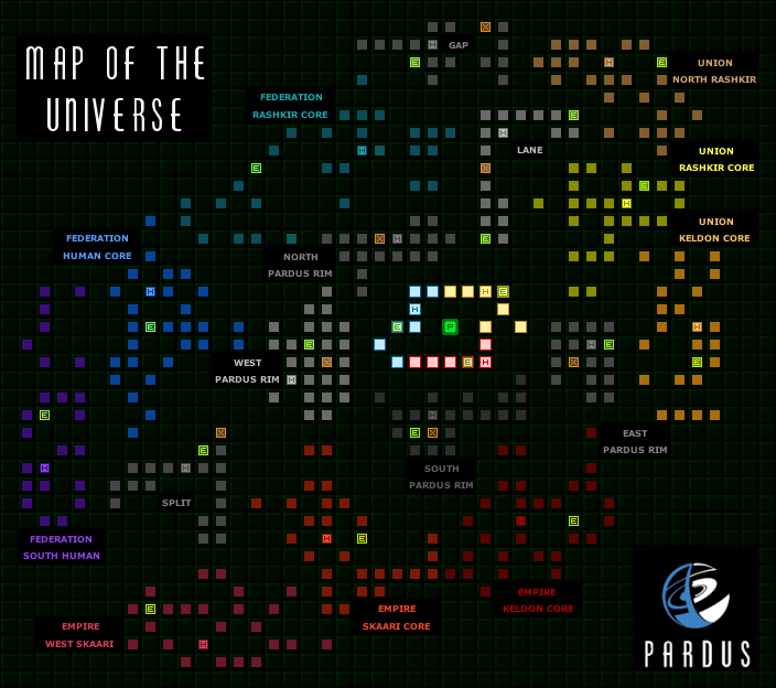
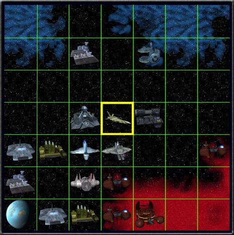
Figure 2: (left) Map of a universe. Squares are sectors consisting of 15$\times$15 fields. Colors indicate clusters. Sectors are connected by wormholes (streets, not shown). (right) Space chart. 7$\times$7 field segment of the universe visible on the players’ navigation screen; the current position is in the center (yellow box). Clicking on another field moves the ship to that location. From [1].

Action Points – the unit of time. Many game actions carried out by a player (trade, travel etc.) cost a certain amount of so-called Action Points (APs). These points can never exceed a maximum of 6,100 APs per avatar. For avatars owning less APs than their maximum, every six minutes 24 APs are automatically regenerated, i.e. 5,760 APs per day. Once a player’s character is out of APs, she has to wait to be able to play on. As a result, the typical player logs in once per day to spend all APs on several activities within a few minutes. This makes APs the game’s unit of time; it is the most valuable factor. Players that use APs most efficiently can experience the fastest progress or earn the highest profits. Social activities, such as communication, do not reduce APs. Highly involved players spend a lot of real time on socializing and on planning their future moves.

2.1.3 Trade and economy

The Pardus currency unit is the so-called credit. It is not convertible to real currencies. Every player starts life with 5,000 credits. Since most objects, such as ships, ship equipment, buildings, are traded in credits, it is of fundamental interest to earn money. There exist a number of possibilities to do this, usually through participation in the economy. The richest players own hundreds of millions of credits. There exist over 30 commodity types. Some of these are renewable and exist in the environment. These “raw materials” can be mined, for example, gas from nebulas or ore from asteroids. Most commodities, however, are processed from more basic ones in player-owned firms. For example, a brewery manufactures expensive liquor out of cheap energy, water, food, and chemical supplies. Every player has the possibility to found a small number of such firms. Production chains follow a fixed production tree, and coordination of several players is needed to establish a sucessful industry. Most end-products at the top of the production tree are usable commodities. For example, manufactured drugs may be consumed to create APs, or droid modules can be installed for powerful building defences against hostile attacks. Needs generated by the society are the driving force behind the development of industries. Besides player-owned firms there are game-owned sites that trade and consume commodities. Prices are exclusively determined by local supply and demand: when commodities are abundant, prices are low, if they are rare, prices rise. Players face an economic life that is known from the real world. It involves collaboration, competition, cartellization, fraud, and so on.

2.1.4 Communication

There are three communication channels in the game: The Chat: players can simultaneously communicate with many others. Chat entries scroll up and disappear; they are good for temporary talks. The Forum: messages, called posts, consist of several lines and stay for a long time. Posts are organized within threads, which bundle into topics. The Private message (PM): a system similar to email, where messages can be sent to any other player. The PM content is only seen by sender and receiver. PMs always have exactly one recipient. These communication channels can be used independently from game-mechanic states, such as ship’s location, wealth, etc. In the following we focus on PMs, and call a PM between two players a “communication event”.

2.1.5 Friends and enemies

For a small amount of APs, players can mark others as their friend or enemy. This can be done for any reason. Marked characters are added to the markers personal friends or enemies lists. Every player also has a personal friend of and enemy of list, displaying all players who have marked them as friend or enemy, respectively. When marked or unmarked as friend or enemy the player is informed. One can mark others as either friend or enemy, not both. Lists are private, meaning that no one except the marking and marked players have information about their ties. In this respect the Pardus system does not introduce a bias toward accumulation of friends, and represents a more realistic social situation, where social ties are not immediately publicly accessible, but have to be found out by communication, or observation of others. The friends and enemies lists also serve game-mechanic purposes: friends/enemies are included/excluded for certain actions. For example, enemies of building owners are not able to use services in the buildings. Friend and enemy markings need not reflect affective relations, they rather indicate a degree of cooperativeness. Friend and enemy relations as well as communication events (PM) are temporal networks, Fig. 3. We denote them by $M^{\rm friend}_{ij}(t)$, $M^{\rm enemy}_{ij}(t)$, and $M^{\rm comm}_{ij}(t)$, respectively.

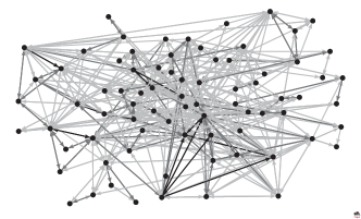
(a) (b)

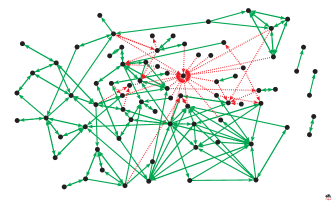
Figure 3: (a) Accumulated communications over 445 days between 78 randomly selected individuals in the early universe, $\sum_{t=\tau}^{\tau+445}M^{\rm comm}_{ij}(t)$. Light gray, gray, and black correspond to 1–10, 11–100, and 101–1000 PMs sent, respectively. (b) Friend (green, solid), $M^{\rm friend}_{ij}(445)$, and enemy (red, dashed), $M^{\rm enemy}_{ij}(445)$, relations on day 445 between the same individuals. One pretty hated guy is visible. From [1].

2.1.6 Performance measures of players—“states”

Players $i$ are characterized by a number of time dependent states, $\sigma_{i}(t)$, that may change as a result of interactions with others. These states can be achievement-factors that quantify various skills of players. The efficiency in harvesting natural resources is quantified by the farming skill, $\sigma_{i}^{\rm farm}(t)$. Other performance measures are combat skill, $\sigma_{i}^{\rm comb}(t)$, that quantifies fighting skills, and the experience points, $\sigma_{i}^{\rm XP}(t)$, that keep a record of fighting and other activities. Players may become members of political factions (parties), which sometimes engage in large-scale conflicts (wars). Faction rank, $\sigma_{i}^{\rm fr}(t)$, is a measure of influence within a faction: above a certain threshold, the faction rank grants the privilege to take part in decisions on war or peace. Finally, players are characterized by a certain wealth level, $\sigma_{i}^{\rm wealth}(t)$, that depends strongly on their economic activities. Some players regard high combat skill, faction rank, wealth, or XP as their main goals in their Pardus life.

2.1.7 Alliances

For various purposes players organize in social groups called alliances. Often players share the same interests, or cooperate in pirate groups, exploration teams, self-defense units, etc. Usually groups do not get larger than about 140 members. Note the proximity to the Dunbar number, 150 [25]. The game provides administration tools for officially declared alliances. Alliances have a common cash pool, which they use for their goals, like defence or production. Often alliances are used for economic purposes. There existed 161 alliances with an average size of 23 members at day 1200. Being a member of an alliance is a social commitment.

3 How do people interact?

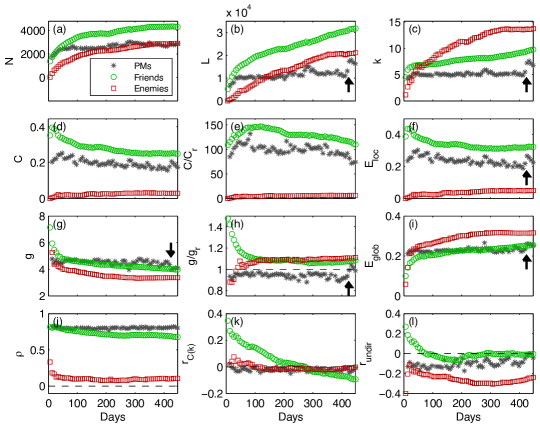
Figure 4: Network properties over time: (a) number of nodes $N$, (b) number of (directed) links $L$, (c) average degree $\bar{k}$, (d) clustering coefficient $C$, (e) clustering coefficient $C$ divided by clustering coefficient of corresponding random graph $C_{\mathrm{r}}$, (f) local efficiency $E_{\mathrm{loc}}$, (g) average geodesic $\bar{g}$, (h) average geodesic $\bar{g}$ divided by average geodesic of corresponding random graph $\bar{g}_{\mathrm{r}}$, (i) global efficiency $E_{\mathrm{glob}}$, (j) reciprocity $\rho$, (k) assortative mixing coefficient $r_{C(k)}$, (l) assortative mixing coefficient $r_{\mathrm{undir}}$. Arrows mark the beginning of a war at day 422. From [1].

One fascinating aspect of this game is that at all times, all social networks are available. Nodes $i$ represent avatars. Links are individual social interactions of type $\alpha$ that happen from player $j$ to player $i$ at time $t$, $M^{\rm\alpha}_{ij}(t)$. This allows us to measure how people interact and organize. We focus on mainly six interaction types:

Communication networks. We consider all PM communications, usually on an aggregated (e.g. weekly) timescale. A weighted link pointing from node $i$ to node $j$ exists if avatar $i$ has sent at least one PM to $j$ within the aggregation period. The weight is the number of sent PMs. Figure 3 (a) illustrates a subgraph of the communication network, accumulated over 445 days between 78 randomly selected characters.

Friends and enemies. A link is defined from $i$ to $j$ if character $i$ has marked character $j$ as friend/enemy. Friend/enemy markings exist until they are actively removed by the players. Friend and enemy networks are unweighted. Since links of friend- and enemy links never coincide, we can see the union of friend- and enemy networks as signed networks. Figure 3 (b) shows a signed friend–enemy network as observed on day 445. Note the cliquishness and reciprocity of friends, and a strong enemy in-hub.

Commercial (trading) networks. Trade networks are extracted by considering two kinds of trading between players: either players meet and exchange credits for commodities, or they visit commercial outlets of other players and buy/sell commodities or equipment there.

Aggression networks. Bounties and Attacks are two forms of how aggression can be expressed in the game. Attack links are defined as attacks carried out by one player on another (or on her commercial outlets). Bounty links represent (weighted) bounties, which are amounts (credits) placed on other players. Any player can collect a bounty by attacking the bountied player, or by harming his commercial outlet.

Other networks in the game are for example production and mobility networks. These do not directly constitute social interactions and will not be of interest here.

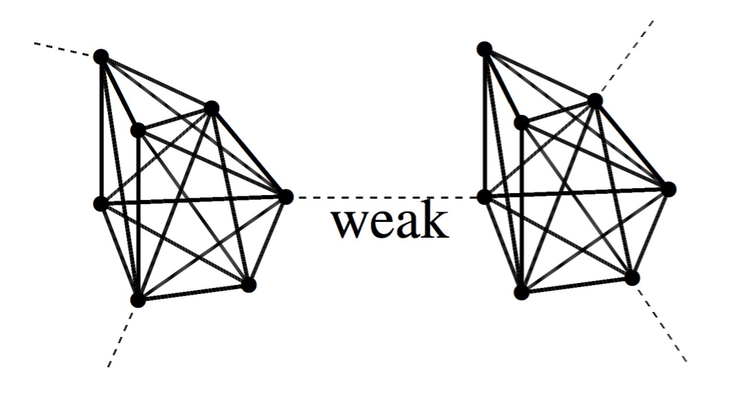
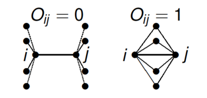
Figure 5: (left) Illustration of what Granovetter means by a weak tie. In network language, weak ties have high link betweenness. (right) Definition of overlap between two nodes $i$ and $j$.

Interaction networks change over time. In Fig. 4 we show a number of network measures as they unfold for communication, friendship, and enmity during the first 422 days, clearly a period in transition. Networks are characterized by growing average degrees, and shrinking diameters; networks densify. After about 1,000 days, most measures become approximately stationary (not shown). Real world communication [21] and friendship networks networks are similar to those observed in Pardus. Not many real world studies exist on enmity networks—people seem to avoid to list their enemies.

3.1 Testing a classic sociological hypothesis of social interaction: weak ties

Given these networks, we can immediately test a classic hypothesis in sociology stated by Mark Granovetter in the 1970s. The so-called the weak ties hypothesis makes a statement about the importance of weak links, that connect communities, see Fig. 5. It states that “the degree of overlap of two individual’s friendship networks varies directly with the strength of their tie to one another”, [17]. Weak ties (for example casual acquaintances) are assumed to be important because they can link communities, which would otherwise be separated. While weak ties are local bridges between communities, strong ties (e.g., good friendships) are easily replaceable intra-community connections. In network language, weak ties are links with a high link-betweenness. Link-betweenness of link $l_{ij}$ is

$$b_{ij}=\sum_{m\in\mathcal{N}}\sum_{n\in\mathcal{N}\setminus{\left\{m\right\}}}\frac{\rho_{mn}(l_{ij})}{\rho_{mn}}\quad,$$ (2)

where $\rho_{mn}$ is the number of all paths between $m$ and $n$, and $\rho_{mn}(l_{ij})$, is the number of paths that contain the link between $i$ and $j$.

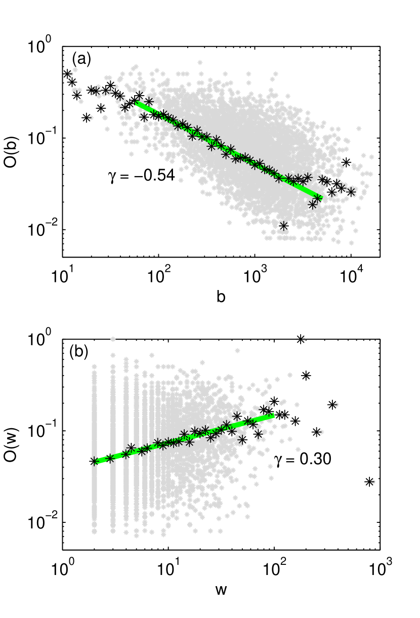
Figure 6: Overlap versus (a) betweenness, and versus (b) weight in largest connected component of the communication network at day 422. Grey markers show individual overlap values of the links. Black markers denote logarithmically binned averages, green lines are least squares fits. From [1].

For testing the hypothesis, we have to clarify how to measure “strength”. We define interaction strength between two individuals as the number of exchanged messages $w=M^{\rm comm}_{ij}(t)$, over a given aggregation period. The hypothesis predicts an increasing function of overlap, $O(w)$ , versus weight $w$. The overlap between two nodes $i$ and $j$ is

$$O_{ij}=\frac{n_{ij}}{(k_{i}-1)+(k_{j}-1)-n_{ij}}\quad,$$ (3)

where $n_{ij}$ is the number of common neighbors of the nodes. The expected relationship is clearly realized for communication networks, see Fig. 6 (b), where we find an approximate cube root law

$$O(w)=w^{0.30}\sim\,^{3}\!\!\!\sqrt{w}\quad.$$ (4)

By the weak ties hypothesis, the overlap $O(b)$, as a function of betweenness, should decrease. Figure 6 (a) confirms this prediction, and suggests an inverse square root law

$$O(b)=b^{-0.54}\sim\frac{1}{\sqrt{b}}\quad.$$ (5)

These results are in agreement with real world communication networks as obtained from mobile phone call data [21], and are robust across game universes and various accumulation times. The weak ties hypothesis was been tested with real small-scale social networks [26]. The weak ties hypothesis is fully confirmed in the Pardus society.

3.1.1 How strong do people interact?—Kepler’s law

We can eliminate the overlap from the equations obtained from Fig. 6, $b=\frac{1}{O^{2}}$ and $w=O^{3}$, and get

$$w^{2}=(1/b)^{3}\quad,$$ (6)

which immediately reminds us at Kepler’s third law of the motion of planets. This relation is interesting in the sense that it relates interaction strength, which is a local quantity between individuals, with the betweenness of a link, which is a global, society-wide quantity: the strength of a (positively connoted) individual relation seems to be related to the structure of the entire network. It remains to be verified if this relation is generally true for real societies.

3.2 Forces between avatars—Newton’s law for social interactions?

In physics there are four fundamental forces, the electromagnetic the weak force, the strong force, and gravitation. The origin of the forces has been clarified in the 20th century. The current view is that they result from the exchange of virtual gauge bosons between interacting particles, see e.g. [27]. Electromagnetism results from the exchange of photons, see Fig. 7 (a), the weak and strong force comes from the exchange of W- and Z-bosons, and gluons, respectively.

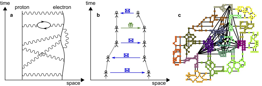
Figure 7: Interactions mediated by exchange of particles. (a) Electromagnetic interaction between a proton and an electron is mediated by the exchange of virtual photons [27]. (b) Two players interact by exchanging messages, $M^{\rm comm}_{ij}(t)$, and goods, $M^{\rm trade}_{ij}(t)$. (c) Map of the universe, where nodes are sectors (cities), lines are connections (wormholes or streets). Colors represent different regions (countries). From [10].

In classical physics a force can be expressed as a negative gradient of a potential $V(\mathbf{x})$

$$m\,a=m\frac{d^{2}}{dt^{2}}\mathbf{x}=-\nabla V(\mathbf{x})\quad.$$ (7)

If a central force is present, meaning that only the distance $r$ between two bodies matters, the potential becomes a function of $r$, $V(\mathbf{x})=V(r)$, and we get

$$ma=-\frac{d}{dr}\left[V(r)+V^{0}(r)\right]\quad,$$ (8)

where $V^{0}(r)$ is an effective-potential. Similar to physics, many human interactions are also based on exchange. Exchanged objects can be messages, goods, money, presents, promises, aggression, bullets, and so on. In Fig. 7 (b) we schematically show the trajectories of two individuals, who exchange messages and a gift; as a result their relative distance reduces over time. Up to now it was not possible to determine if exchange events generate effective attractive or repulsive forces that influence relative motion. This is due to the lack of simultaneous information on exchange events and the trajectories of the involved individuals. This situation is about to change. Data from mobile phone networks, email networks, and online social networks show that the probability for interaction events decays with distance as an approximate power law, $P\sim r^{-\gamma}$ [28, 29, 30, 31, 32, 33, 34, 35, 36], with exponents ranging from $\gamma=0.83$ [35] to $\gamma=2.0$ [28, 29, 30].

Figure 8: Interaction-specific potentials for messages, trade, and attacks. Solid lines are least-squares fits to a harmonic potential in Eq. (9). $V^{0}$ is a result of the background motion of non-interacting pairs of players. The inset is a blow-up for small distances. The potential for attack shows a minimum at $r^{\rm attack}\sim 3$. From [10].

The game is constrained to a 2-dimensional virtual universe that is partitioned into 400 sectors (cities) that are connected by 1,064 local, and 77 long-range connections (roads), see Fig. 7 (c). Movement is not for free, long-distance travel costs more than short moves. Travel can be fast but it takes time; traversing the entire universe needs about three days. We define the distance between two neighbouring sectors as one “step” (network- or Dijkstra distance 1). Given the Dijkstra metric we have relative distances, $r_{ij}(t)$, between players $i$ and $j$, their relative velocities $v_{ij}(t)$, and accelerations $a_{ij}(t)$. At the same time, we have the exchange densities given by the multilayer network, $M^{\alpha}_{ij}(t)$. We can now address the question of how social interactions between humans influence their relative motion. We obtain the interaction potentials by integrating Eq. (8) for cases where particular interactions are predominant. We get

$$V^{\alpha}(r)=\kappa_{\alpha}r^{2}-b_{\alpha}r\quad.$$ (9)

For details, see [11]. The resulting potentials for the three interaction types, communication, trade and attack are shown in Fig. 8. They follow a harmonic and a linear potential, where $\kappa_{\beta}$ is the respective “force constant”. For communication this result is consistent with real-world observations [35]. For trade and attacks, players need to reduce their distance to zero so that an interaction is possible. We see that attractive forces are due to the exchange of messages and trade, whereas repulsive and attractive forces arise from hostile actions (“hit and run” strategy). To confirm this finding in the real world, mobile phone data could be used to perform a similar study.

4 How do people organize?

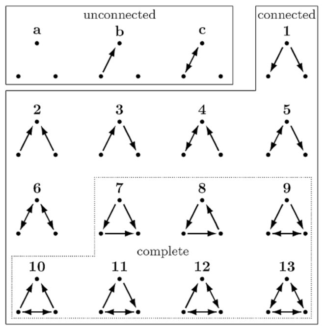
Figure 9: The 16 types of triads and their ids.

4.1 Dynamics of the “atoms of society”: triadic closure

Some sociologists consider triangles (or triads), as the relation between three individuals, as the elementary building block of societies. The fractions of different types of triads within a society provide information about its structure, stability, and efficiency. Granovetter stated in 1973: “The triad which is most unlikely to occur, […] is that in which A and B are strongly linked, A has a strong tie to some friend C, but the tie between C and B is absent.” Again he is talking about friendly interactions. This statement means that one should expect over-representation of closed triads and a suppression of open ones. Does this mean that closed triangles should be under-represented in enmity networks? We will see. For directed networks, there exist 16 types of triads, see Fig. 9. In dynamical terms this means that, over time, open triangles should tend to close. For example, in Fig. 10 we would expect to see triad 6 close to form triad 13. Since we know networks over time, we can count transitions from open to closed triads. The transition counts between all triad types are collected in Fig. 10 (middle).

4.1.1 Testing triadic closure—the triad-significance profile

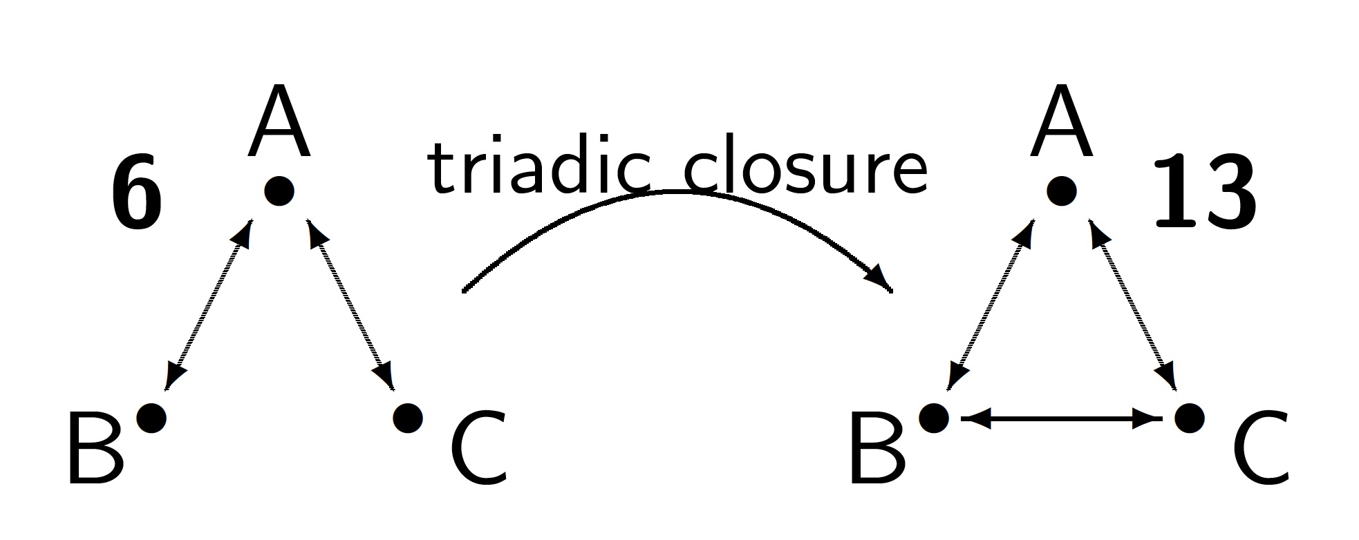
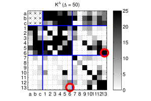
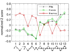
Figure 10: (left) Illustration of triadic closure as the tendency to close open triads. (middle) Transition counts from one type of triad to another. Red circles mark the rates between $6\to 13$, and from $13\to 6$. Clearly, there is a tendency to close open triads. (right) Triad significance profile for the three network types at day 445. From [1].

A way to visualize the over/under-representation of closed triads is to use the $Z$-score. It measures the over/under-representation of specific triads with respect to the number of triads that one would expect in a random graph with the same number of nodes and links. The resulting numbers are collected in the triad significance profile shown in Fig. 10 (right). For friendly interactions, i.e. friendship and communication networks, open triads have negative (normalized) $Z$ scores (under-represented), closed ones are positive (over-represented). We see explicit evidence for triadic closure for friendship and communication networks in Fig. 10. For negatively connoted ties, we find triad types 1–6 over-represented, and 7–13 under-represented in enemy networks. Note the exceptions: triad id 4 is not clearly overrepresented, ids 9 and 11 are not clearly under-represented. If one wants to model social dynamics, triadic closure must be taken into account. We will see in the next section that triadic closure alone is sufficient to explain a number of statistical facts in networks associated with positive interactions. Triadic closure turns out to be a driving force for social network formation, well beyond Granovetter’s initial ideas.

4.2 Taking triadic closure seriously—understanding social multilayer network structure

We now show that triadic closure is able to explain three important statistical facts in three positive networks (communication, trade, and friendship): the degree distribution is an approximate power law with exponent $q$, the node attachment kernel is an approximate power law with exponent $\gamma$, and the clustering coefficient as a function of node degree is an approximate power law with exponent $\beta$.

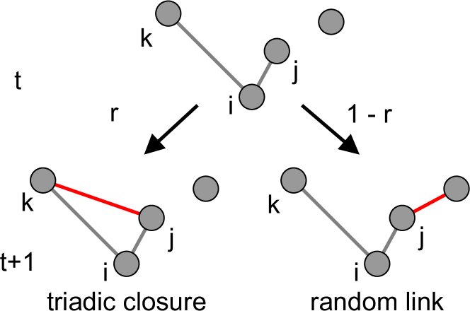
Figure 11: Simple triadic closure model. From time $t$ to $t+1$ a new link is created. With probability $r$ it closes a triangle, with $1-r$ it does not. From [7].

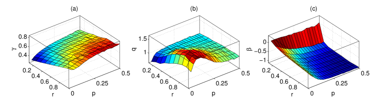
Figure 12: Dependence of scaling exponents $\gamma$, $q$, and $\beta$ on model parameters $p$ and $r$. (a) $\gamma$ increases in $p$ or $r$, and is confined to $0<\gamma<1$. (b) $q$ is large for small $p$ and large $r$; it approaches 1 for large $p$. (c) $\beta$ is close to zero for small $r$, and approaches $\beta=-1$, for large values of $p$ and $r$. $N=10^{3}$, $m=0$, averages over 500 realizations for each $(p,r)$. From [7].

We use a simple model [7] that is shown in Fig. 11. The network is initialized with $N$ nodes, each having one link to a randomly chosen node. The dynamics is completely specified by the iteration of the following steps,

1. Pick a node $i$ at random. If $i$ has less than two links, create a link between $i$ and any randomly chosen node, and continue with step (iii). If $i$ has two or more links, choose one of its neighbors at random, say, node $j$, and continue with step (ii).

2. With probability $r$ (triadic closure parameter), create a link between $j$ and another randomly chosen neighbor of $i$, say $k$. With probability $1-r$, create a link between $j$ and a node randomly chosen from the entire network, see Fig. 11.

3. With probability $p$ (node-turnover parameter) remove a randomly chosen node from the network along with all its links, and introduce a new node linking to $m$ randomly chosen nodes. Then continue with time-step $t+1$.

For $p>0$ nodes have a finite lifetime, which implies that the network reaches a stationary state, where the total number of links $L(t)$, and the network measures $\Pi(k)$, $P(k)$, and $c(k)$ fluctuate around stationary levels. The model is a variation of the model proposed in [37], which appears as the special case for $r=1$, in the above protocol. For similar models, see also [38, 39, 40, 41]. The model is completely specified by four parameters, $N$, $r$, $p$, and $m$, all of which can be read off from the actual game data, i.e. $M^{\alpha}_{ij}(t)$. In this sense, the model does not have a single free parameter. All parameters, including the node- and link-generation rates are obtainable from the game for the three interaction types. The model can now be simulated; the emerging networks are analyzed with respect to the degree distribution, the attachment kernel, and the clustering coefficients.

4.2.1 Characteristic exponents

Simulation results for the values of the characteristic exponents $\gamma,q$, and $\beta$ depend on the parameters $p$ and $r$, see Fig 12. Given $p$ and $r$ (as measured in the data), we can read off the corresponding values of the scaling exponents from Fig 12. These can be compared to the direct measurements from the data, i.e. the model can be validated. Figure 13 shows the attachment kernel $\Pi_{\alpha}(k_{\alpha})$ (the probability for a new node to attach to an existing link with degree $k_{\alpha}$), the degree distribution $P_{\alpha}(k_{\alpha})$, and the clustering coefficients $c_{\alpha}(k_{\alpha})$, for the three sub-networks $M^{\alpha}$ in the empirical multilevel network data. They are compared to the respective distributions of the calibrated model. Data and model agree nicely.

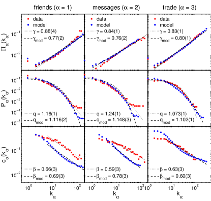
Figure 13: Scaling exponents of the multilayer network as explained by the triadic closure model. Friendship ($\alpha=1$, left column), communication ($\alpha=2$, middle column), and trade ($\alpha=3$, right column). (top row) Attachment kernels scale sub-linearly with the degree in each case. Data and model are barely distinguishable. (middle row) Degree distributions for $\alpha=1,2,3$ and fits to a $q$-exponential. (bottom row) Clustering coefficients as a function of degree for data and model. From [7].

These results suggest that triadic closure may play an even more fundamental role in social multilayer network formation than previously anticipated [42, 17]. Given that all model parameters can be measured in the data, it is remarkable that the three important scaling laws are simultaneously explained by this radically simple model. The exponents found in the model compare well to those of real-world networks. Sub-linear preferential attachment was reported in scientific collaboration networks and the actor co-starring network, $\Pi(k)\sim k^{0.79}$ and $\sim k^{0.81}$, respectively [43]. Degree distributions of many social networks often fall between exponential and power law distributions [44, 45, 21, 1, 46], and scaling of the average clustering coefficients as a function of degree, is observed in scientific collaboration and actor networks, $c(k)\sim k^{-0.77}$ and $\sim k^{-0.31}$, respectively (when the same fitting as in Fig. 13 is applied). Mobile phone and communication networks give $\sim k^{-1}$ [47].

4.3 Degree distributions for negative ties are power laws—positive are not

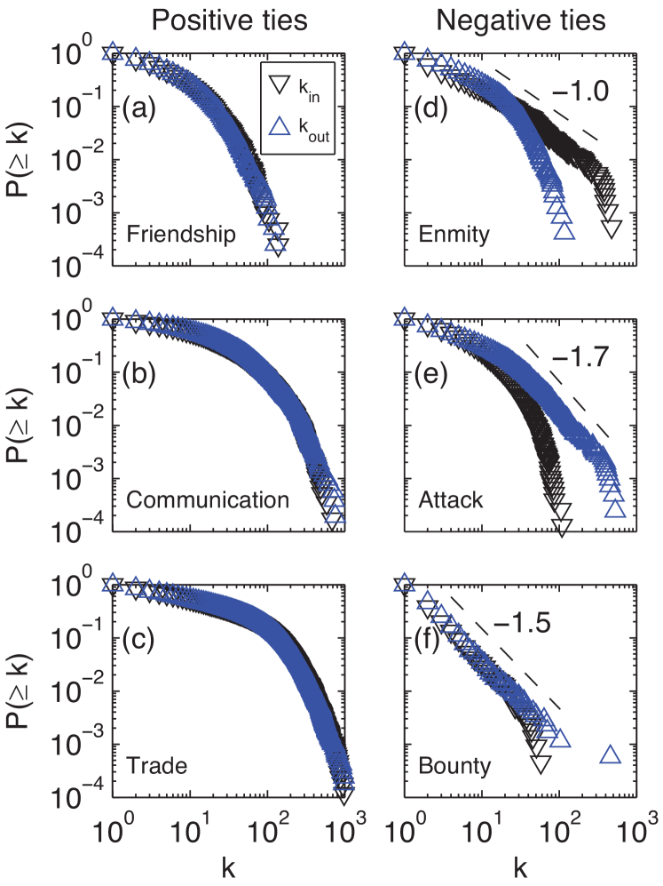
Figure 14: (left) Degree distributions for positive interactions (communication, trade, friendship) follow an approximate Poisson distribution, while negative interactions (enmity, attacks, bounties) show fat tailed distributions that could be power laws (right). From [2].

For the (cumulative) in- and out-degree distributions, we find approximate power laws for aggressive behavior: attacking (out-degree for attacks), being declared an enemy (in-degree for enmity), and punishing/being punished (out- and in- degree for bounty). Power laws are absent for positive (friendship, communication, trade) and passive links (being attacked), see Fig. 14. This suggests different linking/rewiring processes for positive and negative ties. Moreover, we find that positive links are highly reciprocal (directed links go in both directions, $M_{ij}=M_{ji}$), while negative links are not [2]. Low reciprocation in enemy networks may partially be explained by deliberate refusal of reciprocation to demonstrate aversion by total lack of response [1]. For attack networks, it may originate from the asymmetry in the strength of the players (a strong player is more likely to attack someone weaker). We also find that positively connoted links show higher clustering coefficients than negatively connoted ones [2]. High values of clustering are expected for positive interactions because they signal a cohesive structure and seems to benefit performance [48]. The significantly lower clustering for negative interaction types suggests that triadic closure [42] is irrelevant for negative interactions. Their formation might be the result of a “balance” of signed motifs—which is at the core of social balance theory [49].

4.4 Social Balance

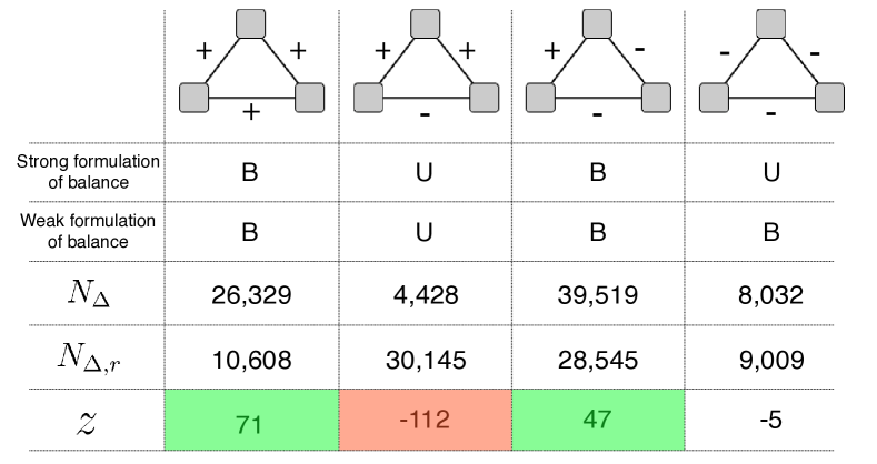
Figure 15: Signed triads, balanced (B) or unbalanced (U), according to the strong or weak formulation of structural balance. We see the number of each type of triad $N_{\Delta}$ in the friendship-enmity bilayer, the expected number of triads in a null model with sign-randomization, $N_{\Delta}^{\mathrm{rand}}$, and the corresponding Z-score (standard deviation from the null model). $+++$ and $+--$ are over-represented, $++-$ are under-represented with extraordinary significance. From [2].

Social balance focuses on signed triads, where the sign is the product of the signs of its three links. In the following we assign +(-)1 to a positive (negative) link, e.g., friendship links have +1, enemy links -1. Social balance theory, in its strong form [50], claims that positive triads are “balanced” and negative triads are “unbalanced”, see Fig. 15. Unbalanced triads are sources of social stress and tend to be avoided. They are therefore under-represented. There is a “weak” formulation of structural balance [51] that assumes that triads with exactly two positive links are under-represented in real networks, while the three other triads should be abundant. In the weak formulation only situations like, “the friend of my friend is my enemy” are unstable, whereas in the strong form of structural balance, “the enemy of my enemy is my enemy” is also unstable, see Fig. 15.

To test social balance, we focus on the bilayer network of friendship and enmity interactions. The number of the different signed triads is $N_{\Delta}$. They are compared to the expected number of such triads in a null model, $N_{\Delta}^{\rm rand}$, where we re-shuffle the signs of links. In Fig. 15 the Z-score shows that $+++$ and $+--$ triads are heavily over-represented, while $++-$ triads are under-represented. Triads of type $---$ are under-represented to a lesser degree than the three other types, favoring the weak formulation of structural balance.

4.4.1 Origin of social balance

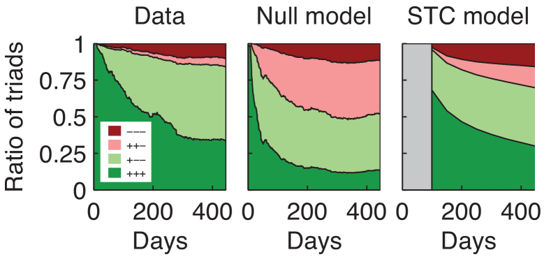
Figure 16: Ratio of signed triads over time as (left) seen in the data, (center) expected from the random null model, and (right) simulation of signed triadic closure. Measured ratios in the data deviate from those in the null model, except for $---$ triads. The model explains the observed ratios much better. From [2].

A dynamical analysis reveals that changes in the network are driven by the creation of new positive and negative links, and not by switching signs of existing links. To illustrate this, we define a wedge as a signed, open triad with two links and one link missing (hole). There are three possible wedge types: $++$, $+-$, $--$. We measure day-to-day transitions from wedges to other triadic structures. For almost all cases ($>99.9\%$), a wedge stays unchanged. In case of change, most often a hole is closed by either a positive or a negative link. Link removal is less frequent, and sign switches almost never occur. This result is in marked contrast with other dynamical models of structural balance [52], which assume that a given social network is fully connected from the start and that link-signs are the relevant dynamical parameters, which evolve to reduce stress in the system. In full agreement with the results in Figs. 15 and 16, wedges of type $++$ close preferentially (about 7 times more likely) with a positive link, wedges of type $+-$ close preferentially (11 times more likely) with a negative link.

We collect empirical transition rates in a transition matrix $A^{\mathrm{STC}}$, which we use in a simple dynamical model for Signed Triadic Closure (STC). $A^{\mathrm{STC}}$ is simply applied on the state vector that contains all signed wedges at time $t$. At time $t+1$, these wedges are either closed or left unchanged. This model reproduces the empirical observations reasonably well, see Fig. 16 (right).

4.5 Avatars organize in multiples of four

Humans dominate their environment by the way they organize in groups. Societies consist of hierarchically layered, nested groups of various quality, size, and structure, such as support cliques, sympathy groups, bands, cognitive groups, tribes, linguistic groups, and so on, [53, 54, 25]. Combining data on human group formation patterns, a discrete hierarchy of group sizes with a preferred scaling ratio close to $3$ was identified [55]. It was later confirmed for hunter-gatherer groups [56] and mammal societies [57]. Do we see such a hierarchical organization in the Pardus society? In particular, do we see the Dunbar numbers?

4.5.1 Dunbar numbers

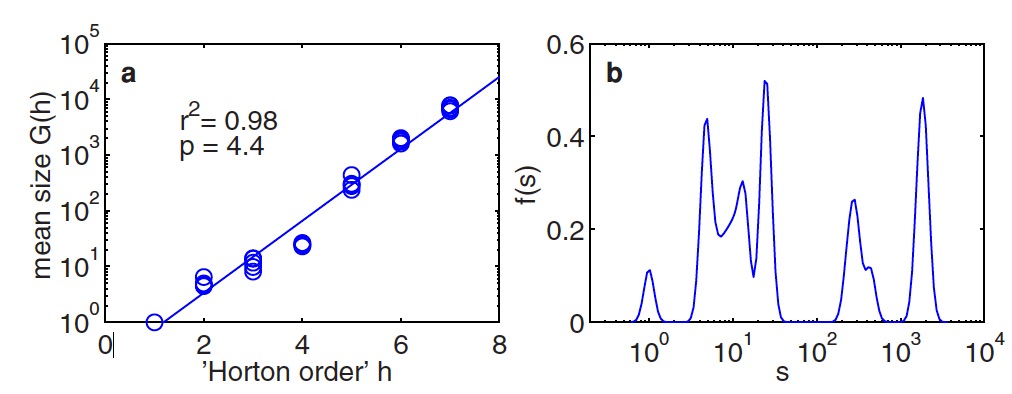
Figure 17: Group size scaling. (a) Horton plot: average size of groups per order. (b) Estimated probability density of group sizes $s$ in Pardus, obtained with a Gaussian kernel estimation ($\sigma=0.14$ acting on the logarithm of group sizes, $\ln(s)$). From [11].

In a nutshell, the concept of the Dunbar numbers is that societies are approximately organized in multiples of three. In its simplest form, this means that groups of size $3$, $3\times 3$, $3\times 3\times 3$, …, $3^{n}$, and so on, should be over-represented. In Fig. 17 we see two indications for that hierarchical scaling. The so-called Horton plot shows the average size of groups per order. These orders have the following, somewhat subjective, meaning. Horton order $h=1$, is the trivial group consisting of one person, the “ego”. Layer 2 ($h=2$) contains closest friends of the ego, defined by both a friendship marking and at least one communication event within the last 30 days. Layer 3 ($h=3$) includes more casual relations, in particular all players that ego has marked as a friend, or by whom ego was marked as friend. Layer 4 ($h=4$) contains the alliance members of the ego. Layer 5 ($h=5$) is obtained by applying a community detection algorithm (Louvain algorithm) [58, 59] to the communication network of the players. We tested that layer 5 is an organisational layer in its own right, whose communities are predominantly subsets of the factions ($h=6$), and supersets of the alliances ($h=4$). Layer 6 ($h=6$) contains the three factions (political parties), and layer 7 ($h=7$) is the entire society. The size of the groups behind these orders scales like a power law with an exponent of roughly $4$, indicating the hierarchical scaling, see Fig. 17 (a). The distribution of group sizes after a smoothing procedure (with a Gaussian kernel) is shown in Fig. 17 (b). It is immediately visible that groups of approximate sizes 1, 4, 16, 30, 250, 1500 are over-represented. This is in line with an hierarchical organization of about four, $4^{n}$, $1,4,16,64,256,1024$. Clearly, this is not a perfect series, and the expected peak at 64 is clearly missing. Hierarchical organisation with a scaling ratio of 3.2 [55], and 3.77 [56], was observed before in real-world societies. The fact that we find these structural patterns in the virtual setting of Pardus, where “life” is detached from most real-world constraints, suggests that this particular form of hierarchical organisation of societies is deeply rooted in human psychology.

4.6 The Behavioral Code

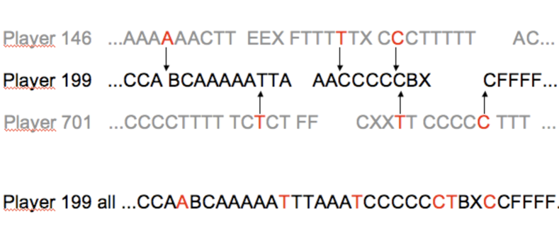
Figure 18: Segment of action sequences of three players. Some actions of players 146 and 701 are directed toward player 199. This results in a sequence of received-actions for 199, $R^{199}=\{\cdots{\rm ATTCT}\cdots\}$. (bottom line) Combined sequence of actions (originated from–and directed to) player 199, $C^{199}$. Red letters mark actions from others to player 199.

To describe a human, one way of doing it is to list the temporal sequence of her actions. In real life there is a huge number of such actions, like cooking coffee, brushing teeth, washing cars, and so on. In the computer game there are much less actions that players can act out. But we have these action sequences ready for analysis. We limit ourselves to eight different actions that every player can execute at any time, and which are observable as changes in $M_{ij}^{\alpha}(t)$. These are communication (C), trade (T), setting a friendship link (F), removing an enemy link (forgiving) (X), attack (A), placing a bounty on another player (punishment) (B), removing a friendship link (D), and setting an enemy link (E). While C, T, F and X are positive (good) actions, A, B, D and E are hostile or negative (bad). We classify communication as positive because only a negligible fraction of communication takes place between enemies [1]. We ignore other possible actions like movement, production, working, sleeping, and so on. Segments of action sequences of three players are shown in Fig. 18.

We consider three types of sequence. The first is the (time-ordered) stream of $N$ consecutive actions $A^{i}=\{a_{n}|n=1,\cdots,N\}$, which player $i$ performs during his “life” in the game. The second is the stream of actions that player $i$ receives from all the other players, i.e. all the actions which are directed towards player $i$. Received-action sequences we denote by $R^{i}=\{r_{n}|n=1,\cdots,L\}$. The third sequence is the time-ordered combination of player $i$’s actions and received-actions, which is a chronological sequence of the elements of $A^{i}$ and $R^{i}$ in their order of occurrence. The combined sequence we denote by $C^{i}$; its length is $L+N$, see Fig. 18. The $n$th element of one of these series is denoted by $A^{i}(n)$, $R^{i}(n)$, or $C^{i}(n)$. We do not consider the actual time between two consecutive actions, which can range from seconds to weeks. We work in “action-time”.

4.6.1 Two ways of seeing the same data

Since individual actions are directed, the information-content of both, the temporal multilayer data, $M_{ij}^{\alpha}(t)$, and the behavioral code ($A$, $R$, $C$) are identical, except that in the latter we use action time. The situation is similar to the Heisenberg- and Schrödinger picture in quantum mechanics. In the multilayer picture the focus is on the topological linking structure, temporal information is hard to visualize (“Heisenberg picture”). In the Behavioral code picture the temporal information is clear, linking structure is harder to visualize (“Schrödinger picture”).

4.6.2 Behavioral code and predicting behavior

By $p(Y|Z)$ we denote the probability that an action of type $Y$ follows action of type $Z$ in the behavioral sequence of a player. $Y$ and $Z$ stand for any of the eight actions, executed or received (received is indicated by a subscript $r$). In Fig. 19 the transition probability matrix, $p\left(Y|Z\right)$, is shown. The $y$ axis indicates the action (or received-action) happening at a time $t$, the probabilities for the actions (or received-actions) that immediately follow are given in the corresponding horizontal place. We find that the probability to perform good actions is significantly higher if in the previous time-step a positive action has been received. Similarly, it is more likely that a player is the target of a positive action, if at the previous timestep he executed a positive action. Conversely, it is highly unlikely that after a good action, executed or received, a player acts negatively, or is the target of a negative action. Instead, if a player acts negatively, it is very likely that he will perform another negative action in the following timestep. Finally, if a negative action is received, it is likely that another negative action will be received in the following timestep. The high statistical significance of the cases $P(-|-)$ and $P(-_{r}|-_{r})$ hints at a high persistence of negative actions in the players’ behavior. For details see [3].

An important finding is obtained by considering pairs of received actions, followed by performed actions. This approach allows us to quantify the influence of received actions on the performed actions. For these pairs we measure a conditional probability of $0.02$ of performing a negative action right after receiving a positive action. This value is significantly lower when compared to the probability of $0.10$, which is obtained from randomly reshuffled sequences. Similarly, we measure a probability of $0.27$ of performing a negative action, right after receiving a negative action. These results agree with a recent study, where the emotional content of posts in online fora was analyzed [60]. The homo sapiens seems to become drastically more aggressive, almost by a factor of ten, immediately after being treated badly.

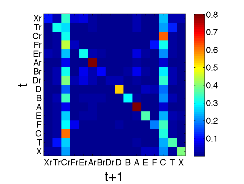
Figure 19: Transition probabilities $p\left(Y|Z\right)$ for actions (or received actions) $Y$ at time $t+1$, given that a specific action $Z$ was executed (or received) in the previous timestep $t$. Received-actions are indicated by subscript $r$. Normalization is such that rows add up to one. Large values in the diagonal show that human actions are often repetitive. Large values for $C\rightarrow C_{r}$ and $C_{r}\rightarrow C$ reveal that communication is an anti-persistent activity—it is more likely to receive a message after sending one, and vice versa, than to send consecutive messages. From [3].

4.6.3 Worldlines of players

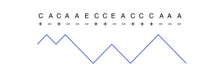
Figure 20: Illustration of a worldline $W_{i}^{\rm good-bad}$ as a binary random walk in “good-bad” action space. Positive actions (C, T, F or X) produce an upward move, negative ones (A, B, D and E) go downward. Good people have rising worldlines.

We can interpret action sequences as random walks. By assigning $+1$ to positive actions C, T, F or X, and $-1$ to negative ones A, B, D and E, we translate a sequence, $A_{i}$, into a binary sequence, $A_{i}^{\rm bin}$. The cumulative sum of the binary sequence is the “worldline” or a random walk for player $i$, $W_{i}^{\rm good-bad}(t)=\sum_{n=1}^{t}A_{i}^{\rm bin}(n)$, see Fig. 20. Similarly, we define binary sequences from the combined sequence $C_{i}$, where we assign $+1$ to an executed action, and $-1$ to a received. This sequence we call $C_{i}^{\rm bin}$; its cumulative sum, $W_{i}^{\rm act-rec}(t)=\sum_{n=1}^{t}C_{i}^{\rm bin}(n)$ is the “action-receive” worldline. Worldlines are shown in Fig. 21 for good-bad action sequences (top), and action-reaction (bottom). Figure 21 (a) also shows that the lifetime of players with many negative actions is often short. The average lifetime for players with a slope $A<0$ is $2,528\pm 1,856$ actions, compared to players with a slope $A>0$ with $3,909\pm 4,559$ actions. The average lifetime of the whole sample of (very active) players is $3,849\pm 4,484$ actions.

To characterize worldlines we define the slope $A$ of the line connecting the origin of the worldline with its end point. It is an approximate measure for “altruism”. $A=1(-1)$ in the good-bad worldlines $W^{\rm good-bad}$ indicates that the player performed only positive (negative) actions. The histogram of the slopes is shown in Fig. 22 (a) for good-bad sequences. For the action–received-action worldline the slope is a measure of how well a person is integrated in her social environment. If $A=1$, the person only acts and receives no input, she is “isolated” but dominant. If $A=-1$, the person is driven by the actions of others and never acts nor reacts. The histogram is shown in Fig. 22 (c).

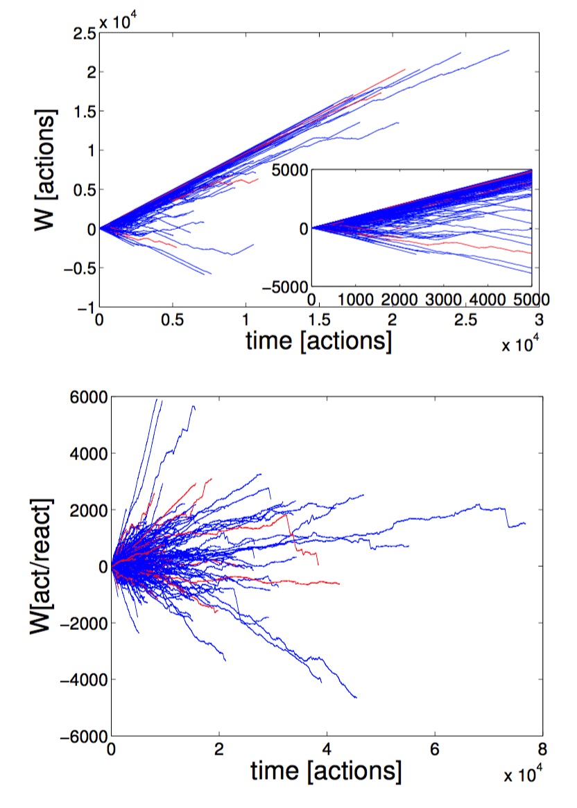
Figure 21: Worldlines of good-bad action random walks (top) of the 1,758 most active players. (bottom) action-reaction worldlines of the same players. Red lines show female avatars.

As a second measure we use the mean square displacement of worldlines to quantify the persistence of action sequences

$$S^{2}(\tau)=\langle(\Delta W(\tau)-\langle\Delta W(\tau)\rangle)^{2}\rangle_{t}\sim\tau^{2\alpha}\quad,$$ (10)

where $\Delta W(\tau)=W(t+\tau)-W(t)$, and $\langle.\rangle_{t}$ is the average over $t$. The asymptotic exponent $\alpha$ quantifies the “persistence” of a worldline. $\alpha=1/2$ is the pure diffusion case, $\alpha>1/2$ indicates persistence, $\alpha<1/2$, anti-persistence. Persistence means that the probability of making an up (down) move at time $t+1$ is larger (less) than $p=1/2$, given the move at time $t$ was up. The histogram of exponents $\alpha$ for the good-bad random walk is shown in Fig. 22 (b), for the action–received-action world line in (d). In both cases persistent behavior is obvious.

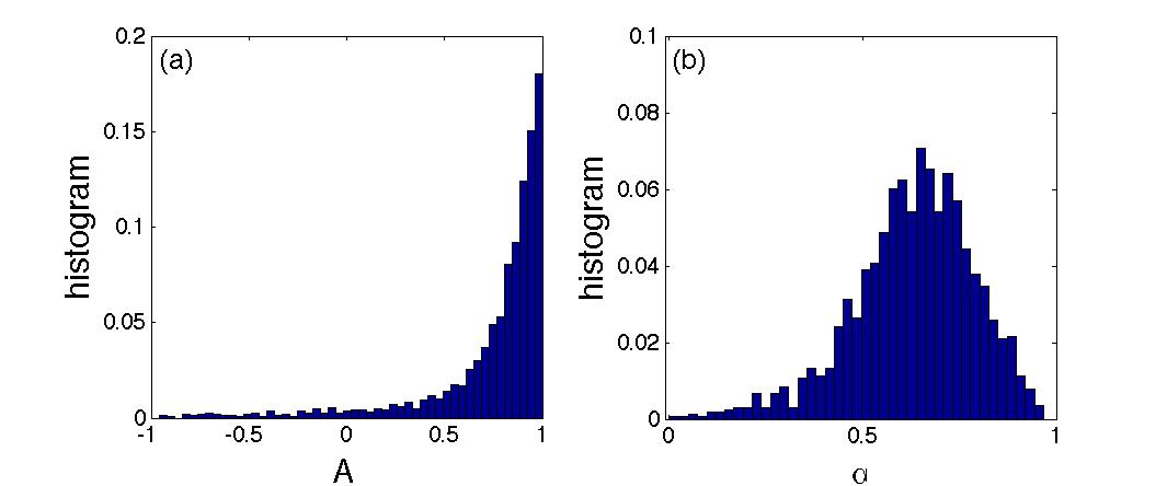
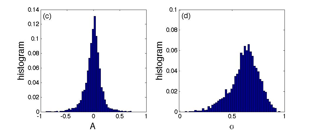
Figure 22: Distribution of worldline slopes, $A$, for good-bad action (a), and action-received action worldlines (c). Distribution of scaling exponents $\alpha$ for good-bad action (b), and action-received action worldlines (d).

4.6.4 Zipf’s law in the human behavioral code

The ensemble of sequences of all actions $A_{i}$ of all players $i$ allows us to analyse the frequencies of the occurring $n$-strings, see [61, 62]. An $n$-string is a subsequence of $n$ adjacent actions in an action sequence. Given our 8-letter action alphabet, (A, B, C, D, E, F, T, X), there are $8^{n}$ different $n$-strings, or “words” $i$, that occur with probability $P_{i}^{(n)}$.

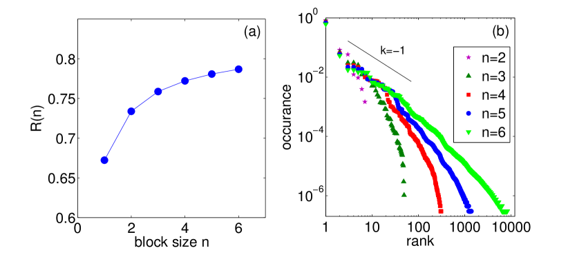
Figure 23: (b) Rank ordered probability distribution of 1 to 6 letter “words” in the 8-letter action alphabet. The slope of $\kappa=-1$ (Zipf’s law) is indicated. (a) Shannon $n$-tuple redundancy increases as a function of word length $n$, a sign for structures in the sequences. From [3].

We partition the action sequences into “words” of length $n$. Fig. 23 (b) shows the rank distribution of word occurrences for different lengths $n$. The distribution shows an approximate Zipf law [61] (slope of $\kappa=-1$), for ranks up to about 100. For ranks between 100 and 25,000, $\kappa\sim-1.5$. The Shannon $n$-tuple redundancy, see e.g. [63, 64], for sequences composed of 8 letters is

$$R^{(n)}=1+\frac{1}{3n}\sum_{i=1}^{8^{n}}P_{i}^{(n)}\log_{2}P_{i}^{(n)}\quad.$$ (11)

For the equi-distribution, $P_{i}=8^{-n}$, we have $R^{(n)}=0$, and in the other extreme of only one single letter in the sequence, $R^{(n)}=1$. Figure 23 (a) shows $R^{(n)}$ as a function of $n$. $R^{(n)}$ increases with $n$, which indicates strong structure in the sequences, since Shannon entropy is not an extensive quantity for action sequences [65].

4.7 Network–network interactions

Social interaction networks of are not independent. How do they influence each other? An answer to this question would contribute much to a deeper understanding of how societies work. We try to take simple first steps in this direction by interpreting several measures that quantify inter-dependencies between pairs of networks. We follow two approaches.

In the first, we focus on the link-overlap between networks and calculate the Jaccard coefficient, $J_{\alpha\beta}$, between two interaction layers $\alpha$ and $\beta$. It measures the tendency that links are simultaneously present in both layers, and is defined as the size of the intersection of the link sets, $\alpha$ and $\beta$, divided by the size of their union, $J_{\alpha\beta}=|\alpha\cap\beta|/|\alpha\cup\beta|$. The link overlap, $O_{\alpha\beta}=\frac{1}{2}\sum_{ij}M_{ij}^{\alpha}M_{ij}^{\beta}$, measures the overlap between networks $\alpha$ and $\beta$. In the second approach, we compute Pearson correlation coefficients, $\rho(k^{\alpha},k^{\beta})=E\left[(k^{\alpha}-\bar{k}^{\alpha})(k^{\beta}-\bar{k}^{\beta})\right]/(\sigma_{k^{\alpha}}\sigma_{k^{\beta}})$, between node degrees in the different layers. They measure to which extent degrees of avatars in one layer correlate with degrees of the same avatar in another. If $\rho(k_{\alpha},k_{\beta})\sim 1$, players who have many (few) links in layer $\alpha$ have many (few) links in layer $\beta$. Note that correlation coefficients might be influenced by different network sizes or different average degrees. To account for this possibility, we additionally compute correlations $\rho(\mathrm{rk}(k^{\alpha}),\mathrm{rk}(k^{\beta}))$ between ranks of node degrees. Overlap and correlation provide complementary views on the organization of social structures. All three measures are shown in Fig. 24 for all possible combinations of network layers. It suggests the following set of conclusions:

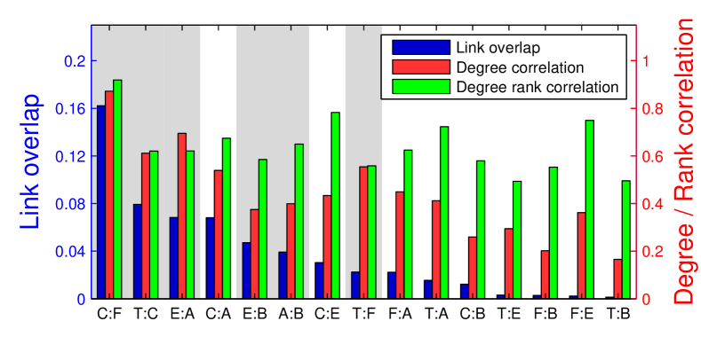
Figure 24: Measures to quantify network-network interactions. Node degree correlation (red), overlap (blue), and rank correlation (green). For an interpretation, see the text. From [2].

Communication–Friendship. The pronounced overlap implies that friends tend to talk with each other, which is of course not unexpected. Strong correlation means that players who communicate with many (few) others tend to have many (few) friends, see also [1].

Trade–Communication. The high overlap shows that trade partners have a tendency to communicate with each other, while high correlations indicate a tendency of communicators also being traders.

Enmity–Attack. The high overlap shows that enemies tend to attack each other, or that attacks are likely to lead to enemy markings. The high correlations imply that aggressors (or victims) tend to be involved in many enemy relations.

Communication–Attack. The relatively high overlap shows that there is a tendency for communication taking place between those players that attack each other. A relatively high correlation implies that players who communicate with many (few) others tend to attack or be attacked by many (few) players. Aggression is not anonymous, but is mostly accompanied by communication.

Enmity–Bounty and Attack–Bounty. The situation is similar to the Enmity–Attack case.

Communication–Enmity. The situation is similar to the Communication–Attack case.

Trade–Friendship. Similar to Trade–Communication, however, with a smaller overlap. It is more difficult for traders to become friends than to just communicate.

Friendship–Attack. The low overlap shows that attacks tend to not take place between friends, or that fighting players do not tend to become friends. The relatively high correlations mean that players with many (few) friends do attack or are attacked by many (few) others.

Trade–Attack. Is similar to the Friendship–Attack case.

Communication–Bounty. Similar to Communication–Attack and Communication–Enmity, however, with much smaller overlap and degree correlations.

Trade–Enmity. For this and all other interactions, overlap vanishes. Players who trade with each other almost never become enemies and vice versa.

Friendship–Bounty. Is similar to the Communication–Bounty case.

Friendship–Enmity. The degree (rank) correlation is substantial, suggesting that players who are socially active tend to establish both, positive and negative links. However, vanishing overlap indicates the absence of ambivalent relations. Friends can not be enemies.

Trade–Bounty. This interaction shows the smallest values for all measures. The relatively small correlation suggests that players who are experienced in trade have a tendency to not act out negative sentiments by spending money on bounties.

The values of the two correlation measures must be interpreted with some care [2]. Low values of $\rho(k_{\alpha},k_{\beta})$ indicate that hubs in one network are not necessarily hubs in another (see e.g. the Trade–Enmity case). This suggests that avatars play very different roles in different network layers. For example they can be central for flows of information but peripheral for flows of goods [66].

5 Gender differences

Figure 25: Players choose a male or female gender when joining the game. Some avatars that players can choose from. All possible avatars come in two genders.

When signing up for the first time, players chose to be a male or female avatar, Fig. 25. We have no information about the biological sex of players. Selecting a gender different from the biological is called gender swapping, which is common in online games [67]. A survey on 8,694 players in Everquest found 15.5% gender-swappers, 17% of the males and 10% of the females [68]. Similar values are reported for Second life (10% swapping of all, 16% of males, 2.7% of females) [69], or for World of Warcraft (23% of males, 3% of females) [70].

We observe that on average females are less risk-taking but wealthier [6]. Females accumulate significantly more wealth (4 sigma level) than males. At the same time, male players experience significantly more deaths (2 sigma level), due to more risk-taking and/or aggressive behavior. This points to a much larger engagement of females in economic, rather than destructive activities. Concerning overall activity, experience points, kills and collected bounties, female and male players perform comparably ($H_{0}$ can not be rejected).

Females show homophily, males are heterophiles [6]. Homophily is the tendency of individuals to associate and link with similar others [71]. A straightforward way to measure homophily is to compare the numbers of directed links between all gender-combinations (MM, MF, FM, FF) in all network layers to the corresponding numbers from surrogate data, where the gender of nodes is randomized (re-shuffled) but the topology of the network is left intact. To measure statistical significance of differences between the various combinations of genders, we compare each real network to 1,000 reshuffled surrogate networks. Female-to-female trading and communication are the most significantly over-represented link types, with a Z-score of approximately 4 sigmas [6]. Male-to-female trades ($Z=2.7$) and communication ($Z=2.7$) are also strongly over-represented, whereas the opposite, female-to-male trades and communication is much less substantial ($Z=1.4$ and $1.6$, respectively). Male-to-male trades and communication are under-represented ($Z=-2.3$ for both cases). Negative link types show no significant homophily in either direction.

5.1 Gender differences in networking

How do male and female players create and manage their local networks? Are they different?

5.1.1 Gender differences in network topology

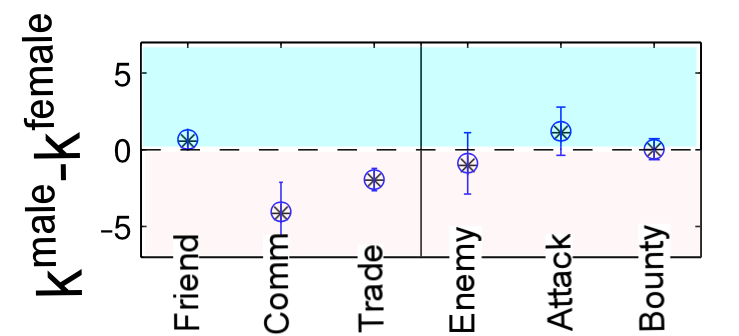
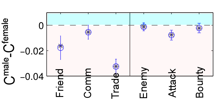
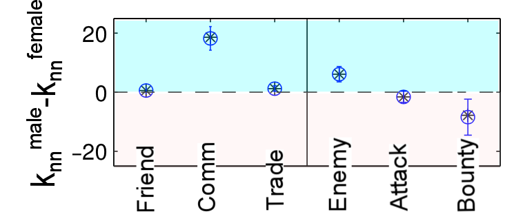
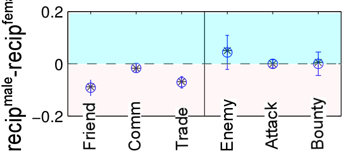
Figure 26: Network differences for male and female players on day 856 (male minus female). (a) average degree ${k}$, (b) clustering coefficient $C$, (c) average neighbour degree ${k}^{nn}$. Females have higher average degrees in communication and trade networks, as well as a higher clustering coefficient in trades, but considerably lower ${k}^{nn}$ for communication. (d) reciprocity between male-male and female-female links. Females are much more reciprocal in friendships and trades. Errorbars are standard deviations of the network measures obtained from 8 male control groups, each of the same size as the female sub-group.

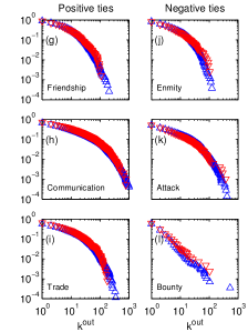
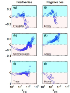
Figure 27: (left panel) degree distributions for six social interaction layers for males (red) and females (blue). (right panel) differences (male minus female) out-degree, plotted against the degree. Gender differences become apparent. Female players appear to be super-likers, and super-haters. Females have more communication partners for almost all degrees. For aggression-management, males prefer attacks, females prefer bounties—at all degrees. From [6].

Figure 26 shows gender differences in four network properties as observed on day 856, illustrating that males and females structure their local network layers in very different ways. We compute the average degree ${k}$, the clustering coefficient $C$, and the average nearest neighbour degree $k^{\mathrm{nn}}$. We then subtract the value for the female group from the average of 8 male control groups of equal size. This difference is shown in the panels. Errorbars are the standard deviations of the means of the control groups. We find the following differences:

Females have more communication partners. As seen in Fig. 26 (a), on average females have about 5 more communication and 2-3 more trading partners than males.

Females organize in clusters. Female trading networks show a clustering coefficient that is much (about 25%) higher than the one of males, Fig. 26 (b). This means that females tend to trade with people who trade among themselves. Also the clustering of female friendship networks is significantly higher than those of males, showing a preference for stability in local networks [17]. Surprisingly, also for attacks females are more likely than men to attack people who are already in conflict with each other.

Males prefer well-connected communication partners. From Fig. 26 (c) we learn that the communication partners of males have more communication partners than the communication partners of females. The same tendency is seen for male enmity networks, meaning that the typical enemy of a male player has more enemies than the typical enemy of a female. In relative terms, both effects are in the 10% range [6].

Females reciprocate friendships. Females invest more effort in reciprocating positive links. Figure 26 (d) shows that females reciprocate more friendship and trading links than males. For most negative links, there are no substantial gender differences.

On average, females have 5 more communication partners, females build more triangles, males link to well-connected communicators, and females reciprocate more. This has practical consequences for social life: while females focus on stable structures (high clustering), males seem to optimize communication speed by linking to well-connected communication partners. Male networks are less stable, but information spreads faster.

In the left panel of Fig. 27 we compare degree distributions of the different interaction layers, for females (red) and male (blue). In the right panel we see the degree-differences as a function of the degree. These plots illustrate that women are super-communicators (dominating, whenever many friends are involved), and females are the super-enemies (whenever the degree in enmity networks becomes very large). Males play out aggression though attacks, while females prefer bounties to manage their negative feelings towards others—at all degrees.

5.1.2 Gender differences in temporal behavior

Imagine one player marks another as a friend. How long does it take to respond to this action? We can measure the time-to-respond to any action that is directed from one player to another. Males appear to respond fast (slow) to female friendship (enmity) initiatives. We measure the time-to-reciprocate (ttr) it takes for individuals to reciprocate actions of a given type. In Fig. 28 (a) and (b) we show the cumulative distributions for the time-to-reciprocate for friendship and enmity links, for the four possible gender permutations: MM, FF, MF, FM. The first letter denotes the gender of the initiator, the second of the reciprocator. The decay rate $\lambda$ for MF friendship reciprocation is $\lambda_{\mathrm{MF}}\sim-0.0060$. For female initiation and male reciprocation it is $\lambda_{\mathrm{FM}}\sim-0.0078$. The MM rate is similar to the FM case, $\lambda_{\mathrm{MM}}\sim-0.0075$ (b). Correspondingly, the half-life for MF reciprocation is about 116, for FM it is only 89 days. The situation changes for enemy links. Here a difference is found within the first 150 days of an enemy marking: males reciprocate much faster than females. The approximate rates are $\lambda_{\mathrm{FM}}\sim-0.0065$, and $\lambda_{\mathrm{MF}}\sim-0.0055$, respectively.

In summary, we see that males respond fast to female friendship initiatives—females slow to male ones. Females respond fast to female friendship initiatives—males slow to males ones. And finally, males respond fast to enemy activities from males—but respond slow to female aggression

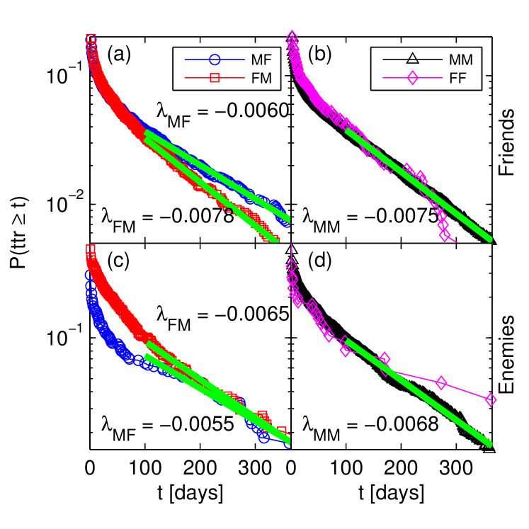
Figure 28: Time-to-respond distributions for different gender combinations. (a) Time for females to reciprocate a friendship link from a male initiator (MF), and vice versa (FM). On long time scales ($>30$ days), males are much faster to reciprocate female friendship initiatives than the other way round. (b) Equal sex reciprocation MM, and FF. Decay times are somewhere between the MF and FM case. (c) Time-to-respond for enemy links. Males are considerably slower to reciprocate within the first 180 days if the initiator was a female than the other way. (d) Equal sex reciprocation for enemy links.

6 Mobility—how avatars move in their universe

Pardus is a world with a well-defined space. Players can move on a 2-dimensional surface, see Fig. 7 (c). Since we know the location of all avatars at any point in time, we can study mobility patterns, and compare them to those of humans on the 2-dimensional surface of Earth. We locate players in one of the $N=400$ nodes, the so-called sectors (cities), that are linked by $K=1160$ wormholes (roads). Sectors are arranged into 20 different clusters, which are perceived by the players as different political or socio-economic regions, similar to countries. Each cluster is shown with a different background color in Fig. 7 (c). Players usually have a “home cluster”, where they focus their socio-economic activities over long time periods. Occasionally, they move to sectors belonging to other clusters to explore the universe, to relocate their home (migrate), or in response to extreme events, such as wars.

6.1 Jump- and waiting time distributions

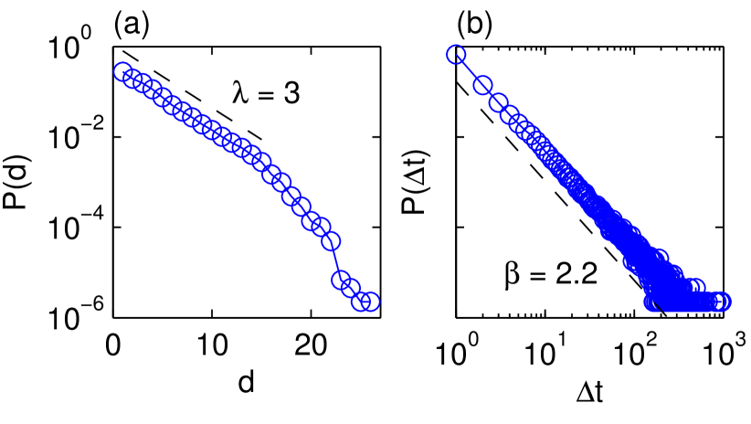
Figure 29: Distribution of jump distances $d$ (a), and waiting times $\Delta t$ (b). A jump occurs whenever the sector position changes from one day to the following. The distribution of jump distances has a characteristic length of $\lambda\sim 3$. The waiting time $\Delta t$ is the number of consecutive days a player spends in the same sector. The distribution is an approximate power law with an exponent of $\beta\sim 2.2$. From [4].

In Fig. 29 we show the distributions of jump (travel) distance and the waiting times between movements (jumps) from players’ trajectories over 1,000 days. In Fig. 29 we show the distributions of jump (travel) distance and the waiting times between movements (jumps) from players’ trajectories over 1,000 days. The length $d$ (integer) of a jump is measured in terms of network distance, and ranges from 1 to $d_{\mathrm{max}}=27$, the diameter of the network. The distribution of jump distances for all players over the observation period, is seen in Fig. 29 (a). For $d\leq 15$, the distribution is approximately exponential

$$P(d)\sim e^{-\frac{d}{\lambda}}\quad,$$ (12)

with a characteristic jump length of $\lambda\sim 3$. The existence of a typical travel distance was found in real-world mobility data [72, 73]. The distribution of waiting times, $\Delta t$ (in days), between all consecutive jumps is seen in Fig. 29 (b). It follows an approximate power law

$$P(\Delta t)\sim\Delta t^{-\beta}\quad,$$ (13)

with $\beta\sim 2.2$, in agreement with recent measurements on human mobility [74]. We find that mobility patterns are strongly influenced by the presence of clusters, the socio-economic regions [4].

6.2 Long-term memory and mobility

To understand the diffusion of avatars over the transport network, we show the mean square displacement (MSD) of their positions in Fig. 30 (a), $\sigma^{2}(t)\sim t^{\nu}$, with $\nu\sim 0.26$. This indicates anomalous, sub-diffusive behaviour. This is not an effect from the specific topology of the Pardus universe. To see this, in Fig. 30 (b), we show the situation for random walkers on the wormhole network (gray stars). It produces the expected MSD result that is expected from standard diffusion, i.e. with an exponent $\nu\sim 1$, for up to $t\sim 100$ days, at which the fine size of the universe begins to play, which causes the saturation. We tested several potential models to explain the anomalous diffusion behaviour, including a simple Markov model that is based on the observed node–node transition probabilities, and a preferential-return model that takes higher-order memory effects into account [75, 76]. Both are not able to capture the correct scaling pattern of the MSD, in particular $\nu\sim 0.26$, as seen in Fig. 30 (b).

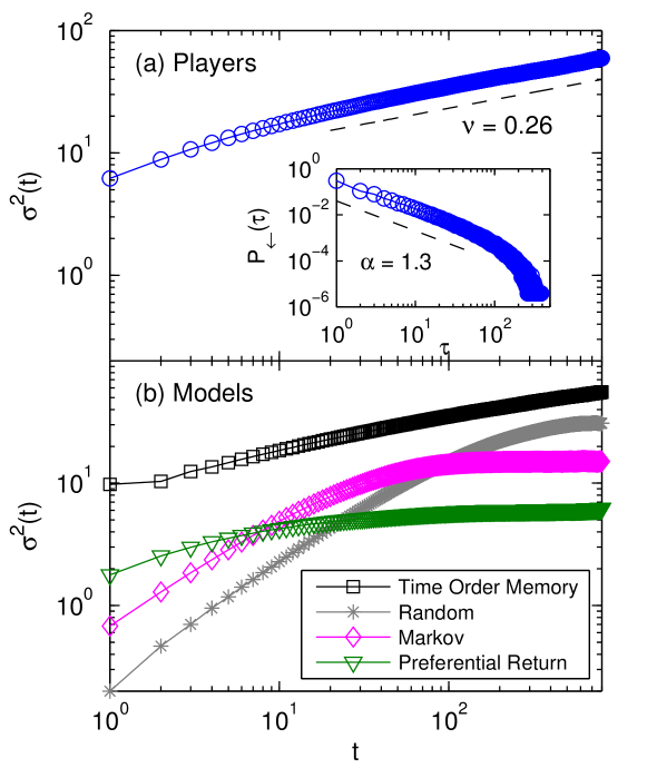
Figure 30: (a) Mean square displacement (MSD) of players’ trajectories follows a power law, $\sigma^{2}(t)\sim t^{\nu}$, with sub-diffusive exponent $\nu\sim 0.26$. The inset shows the probability, $P_{\hookleftarrow}(\tau)$, for a player to return to a previously visited sector after $\tau$ jumps. (b) MSD for various models to explain the observed scaling exponent $\nu$. Random walkers, a Markov model, and a preferential return model can not explain $\nu$. A model with long-time memory (Time Order Memory) reproduces the exponent almost perfectly. Curves are shifted vertically for clarity. From [4].

The reason for failure is that the probability to move to a certain location does not depend on the current location, nor on the order of previously visited locations. Instead, we observe that individuals tend to return to sectors they have visited recently. To model this mechanism we measure the return time distribution in the jump timeseries for returning (for the first time) to the currently occupied sector after $\tau$ jumps, and find $P_{\hookleftarrow}(\tau)\sim\tau^{-\alpha}$, with $\alpha\sim 1.3$, see Fig. 30 (a). We use this information to design a “Time Order Memory” (TOM) model that incorporates a power law distribution of first return times, power law distributed waiting times, and exponentially distributed jump distances. These ingredients are sufficient to reproduce the sub-diffusive behaviour in Fig. 30 (a). The model works as follows: an individual rests in a given sector for a number of days drawn from the waiting time distribution. Then, she jumps. There are two possibilities: (i) with probability $v$ she returns to an already visited sector, (ii) with probability $1-v$ she jumps to a sector she never visited before. For (i), one of the previously visited sectors is chosen with $P_{\hookleftarrow}(\tau)$. In case (ii), she draws a distance $d$ from the distance distribution, and jumps to a randomly selected sector at that distance. The model parameters, $\lambda$, $\beta$, and $\alpha$, are all fixed by the data. By averaging over all jumps and players, the probability of returning to an already visited location is found as $v\sim 0.83$. We get $\nu_{\mathrm{TOM}}=0.23\pm 0.02$, in agreement with the observed exponent. Black squares in Fig. 30 (b) indicate that the model works indeed.

In summary, we find that mobility in the Pardus world is not all that different from mobility on Earth. Locations are visited in specific temporal patterns, leading to strong memory effects that are essential to understand the statistics of observed mobility trajectories. Neglecting either spatial or temporal factors make it hard to understand the statistics of human mobility. This might be true in the real world too. Interestingly, a thorough understanding of human mobility is still outstanding, since some results appear to be contradictory [77]. Some report fat-tailed distributions of trip lengths [78, 76], others exponential or binomial distributions [73, 72, 77].

7 The wealth of virtual nations

Almost universally, wealth is not distributed uniformly within societies. Even though wealth data have been collected in various forms for centuries, the origins behind wealth-, and hence, social inequality are not yet fully understood. This is not different in Pardus. However, there we can figure out what it needs to be wealthy in terms of your position in the social multilayer network. Can we finally understand the origin of wealth inequality?

7.1 More on the Pardus economy

From interaction data, $M_{ij}^{\alpha}(t)$, and player states, $\sigma_{i}^{\rm X}(t)$, we can reconstruct all economic activities in the Pardus society. In particular the input-output production matrix of the economy and the variety of goods are pre-defined. Goods are of uniform quality (homogeneous); consumables and equipment can be partially substituted by other types of consumable and equipment. Intermediate goods are needed for production in exact proportions. There are 5 commodities (natural resources), 19 intermediate goods, and 5 end-products, i.e. consumables. Although capital requirements to establish production facilities are low, there are barriers to entering production. Incumbents may threaten or harm potential new entrepreneurs. Game rules set a maximum number of production facilities per player. Production facilities can not be sold. Investments in production facilities therefore motivate players to stay in the sector. No labor is needed for production itself, but transport of raw materials and intermediate goods requires effort and resources. Because of transport costs, facilities effectively only compete with similar facilities nearby. This leads to local oligopolies. Owners of production facilities are completely free to set the price at which they sell their products. There exist non-player facilities (belonging to the game) whose prices depend on local supply and demand. The monetary currency is called credits. There is no credit or banking system, all transactions are payed and cleared immediately. There is no inflation.

7.2 Wealth

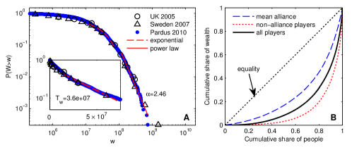
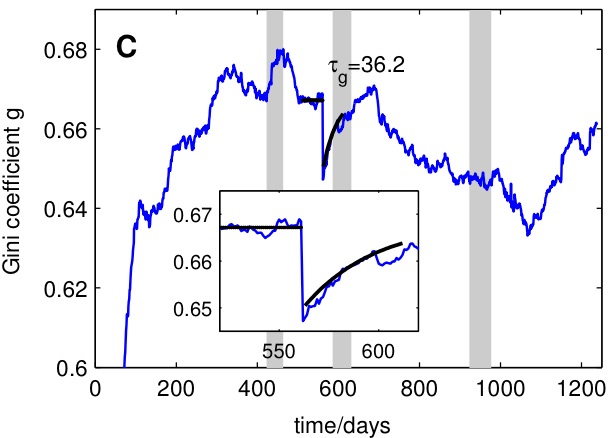
Figure 31: (a) Cumulative wealth distributions for Sweden, the UK, and for the Pardus society on day 1200. Note the similarity. (b) Corresponding Lorenz curve of wealth in Pardus. For every alliance, a separate Lorenz curve is calculated; the dashed blue line is their average. (c) Gini index over time, $g(t)$. A Christmas charity event on day 562 leds to a re-distribution from the wealthy to the poor, resulting in a downward jump of the Gini index. The inset shows the exponential recovery to previous levels. Gray areas indicate periods of war. From [12].

There are various ways to accumulate wealth: trading, collecting and selling natural resources, producing goods, working for hire (common jobs are courier, hunter, or bounty hunter), receiving donations or other payments, increase of the alliance funds, robbing, and stealing. The wealth of player $i$ is the sum of the value of his assets, cash $v_{l,i}$, equipment $v_{e,i}$, share of alliance funds $v_{af,i}$, and inventory $v_{inv,i}$; details in [12],

$$\sigma_{i}^{\rm wealth}(t)=v_{l,i}(t)+v_{e,i}(t)+v_{af,i}+v_{inv,i}\quad.$$ (14)

Ways to reduce wealth include consumption, paying for maintenance, investing in production facilities or equipment, discarding goods, becoming victim of theft or robbery, giving to fellow players, or paying into alliance funds, a decrease of the alliance funds, or making adverse trades.

The cumulative wealth distribution of Pardus players, in comparison to the UK and Sweden, is shown in Fig. 31 (a) New and inactive players were excluded. The bulk of the distribution is compatible with an exponential with decay $T_{w}=3.6\times 10^{7}$ credits. The tail can be seen as an approximate power law with exponent $\alpha\sim 2.5$. The situation is compatible with real world data [79].

7.3 Inequality

Figure 31 (b) shows the Lorenz curve for the Pardus society (black line). It is the share of the total wealth as a function of the fraction of the people holding that share. The closer the Lorenz curve is to the diagonal (black dotted line) the more egalitarian is the wealth distribution. Uniform wealth distribution corresponds to the diagonal. Associated to the Lorenz curve is the Gini index, $g=1-2A$, with $A$ being the area (integral) under the curve [80]. We find $g=0.65$. We show the Lorenz curves for all players and for those that are not organized in any alliance (red dotted line). These players generally operate individually, and show a much more pronounced wealth inequality than the entire society, the respective Gini index being $0.70$. In contrast, the Lorenz curve for the various alliances (dashed blue line) indicates that people within the alliances tend to be much more equal in wealth, when compared to the entire society. The Gini index for the alliances is $0.50$. The main reason for this higher equality is the smaller fraction of poor players in alliances: while $79\%$ of the total population, and $92\%$ of the richest $10\%$, are alliance members, only $28\%$ of the poorest $10\%$ are.

Figure 31 (c) shows the time evolution of the Gini index. After an initial steep rise in the first 150 days, the Gini index $g$ fluctuates between $0.68$ and $0.63$, similar to many Western countries. A sharp drop of $g$ from $0.67$ to $0.65$ occurred on Christmas day 2008. On this day, a charity event took place, where thousands of players donated cash for the less wealthy. The gained level of equality is lost exponentially fast, within a few days previous Gini index levels are reached, see inset. This indicates a remarkable stability of the shape of the wealth distribution. It is hard to decrease inequality by re-distributing wealth. Is the origin of wealth inequality based in social behavior?

7.4 Behavioral factors for wealth

7.4.1 Influence of activity on wealth

We see a trivial strong linear relation between the average wealth of a player and her total activity. The corresponding Pearson correlation coefficient is $\rho=0.535$ ($p$-value $<10^{-6}$). We conduct a partial correlation analysis and find several significant behavioral factors that explain wealth [12]. We find that the more a player trades compared to his other actions, the higher is his wealth-gain. This is not surprising since trade is the main source of income in the game. We also find that the more of a player’s actions are attacks, the lower is his wealth-gain. This suggests that revenue from attacks through robbery and bounty hunting does hardly bear the associated costs, e.g. for repairing damage caused by fights. There might be secondary damaging effects of aggressive behavior, such as reduced willingness of others to socialize (and trade) in the future. Another explanation might be that attacks are sometimes carried out without economic interests, but just for creating terror.

7.4.2 Influence of achievement-factors on wealth

Wealth and other achievement factors, such as skills, XPs, and faction rank, are strongly correlated with total activity. For this reason, we define the wealth-gain of player $i$ as $\eta_{i}(t)=w_{i}(t)/a_{i}(t)$, where $a_{i}(t)$ is the cumulative activity of a player approximated by the total amount of APs he has “spent”. $\eta_{i}(t)$ can be seen as the efficiency of gaining wealth. To further exclude these spurious correlations, partial correlation coefficients are calculated. Age and faction rank are a significant factors ($p$-value below 1%). Players that are not in any faction, i.e. on average less social, have the smallest possible value of faction rank, and are generally poorer. There is a significant fraction of rich people with low combat skill. Otherwise, we find no correlation between combat skill and wealth-gain. Farming skill has a consistently positive and mostly significant correlation with wealth.

In Fig. 32 we show the wealth-gain as a function of a combination of different performance factors. High farming skills and intermediary combat skills correlate with high wealth-gains that are shown as by colors (high wealth-gain is red). Below a certain level of experience points, no high wealth-gain seems possible, and a high faction rank together with high experience point scores are a good predictor for wealth. For details, see [12].

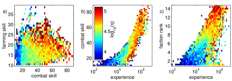
Figure 32: Two-dimensional binned averages of the wealth-gain as a function of achievement-factors. Colors represent the logarithm of the average wealth-gain, $\log_{10}(\eta)$, over all players that fall into that bin. Blue corresponds to low, red to high values, empty bins are white. A XP and faction rank, B XP and combat skill, C combat skill and farming skill. From [12].

7.4.3 Wealth depends on how social you are

Alliance members on average are somewhat richer than non-alliance members, both in absolute terms and in wealth-gain. Members also have better skills and a higher faction rank. As seen in Fig. 33 the size of an alliance has little influence on wealth and other factors, except for players that are in no alliances or in alliances with only two members. These players are consistently poorer than players in groups with three and more members. Members of the largest alliances show performance indicators below average (dashed line). It does not matter if you are member of big or small groups; it matters if you are a member of at least one group.

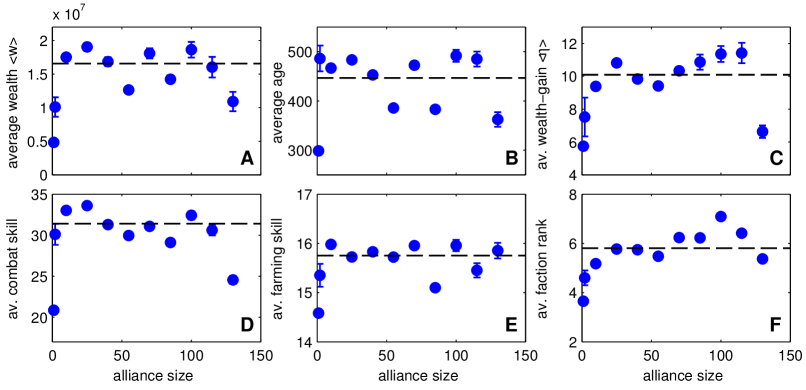
Figure 33: (a) Wealth, (b) age, (c) wealth-gain, (d) combat skill, (e) farming skill, (f) faction rank as a function of alliance size. The first bin contains players that are in no alliance, the second bin has players in alliances of size two. Members of the smallest alliances show low wealth and achievement scores. Also the largest groups show lower levels. The line is the average over all players in alliances with at least three members. From [12].

7.5 Wealth and position in the multilayer network

We use the trade, communication, friendship, and enemy interactions layers, $M_{ij}^{\alpha}(t)$, to determine the in- and out-degree, $k^{\mathrm{in}}_{i}$ and $k^{\mathrm{out}}_{i}$, the nearest-neighbor degree, $k^{\mathrm{nn}}_{i}$, and the clustering coefficient, $c_{i}$, for every player $i$. To show the dependence of wealth-gain on various combinations of these network parameters, we plot two-dimensional binned averages of wealth-gain versus pairs of network measures in Fig. 34. The color is the logarithm of wealth-gain, $\log_{10}(\eta)$, from blue (lowest) to red (highest). We find the following results:

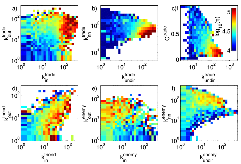
Figure 34: Wealth-gain ($\log_{10}(\eta)$) as a function of network properties, blue (lowest) to red (highest), empty bins are white. (a) trade in- and out-degree, (b) trade undirected degree and nearest-neighbor degree, (c) trade undirected degree and clustering coefficient, (d) friend in- and out-degree, (e) enmity in- and out-degree, (f) enmity undirected degree, and nearest-neighbor degree. From [12].

Trade. The trade layer has the strongest impact on wealth. Trade in-degree has a significant, positive partial correlation with wealth. The in-degree is defined as trade with a player’s production facilities and is therefore a proxy for his production. Figure 34 (a) confirms the positive connection between trade in-degree and wealth, while showing much less influence from trade out-degree. Concerning the undirected degree of the trade network versus the nearest-neighbor degree (b), we see that the richest are found to have an intermediate nearest-neighbor degree of about $k^{\mathrm{trade}}_{\mathrm{nn}}\sim 35-70$, well below their undirected degree. This means that they are selling to people that are less connected in the trade network than they are themselves. From Fig. 34 (c) we gather that high wealth-gain is made with a combination of high degree and a relatively low clustering coefficient, $C^{\mathrm{trade}}\sim 0.1$. This means that rich players avoid cyclical structures in their trading networks, which allows them to act as “brokers” between players that do not directly trade with each other. The partial correlation between wealth and the trade clustering coefficient is negative.

Communication. Communication in-degree has a significantly positive partial correlation. High communication in-degree means good access to information, which is expected to be profitable. Since communication links are reciprocal, and in- and out-degree are highly correlated, there might be a spurious effect of the communication in-degree. The communication nearest-neighbor degree has a negative and mostly significant partial correlation. This might indicate that it is advantageous to converse with players who are less informed than oneself.

Friendship. In Fig. 34 (d) the situation for the in- and out-degrees for the friendship layer is shown. Players with high wealth-gain are those that are liked by more players than they like themselves, $k_{\mathrm{in}}^{\mathrm{friend}}>k_{\mathrm{out}}^{\mathrm{friend}}$. Poor players have marked others as friends more often on average than they are marked. The role of these asymmetries might be a fruitful direction for future study.

Enmity. We see that people with above-average wealth-gain are rarely marked as an enemy by others, but do mark others as enemies, (e). Players who have been marked as enemy by many others are generally poor. In agreement with this finding, the enmity in-degree has a significant negative partial correlation with wealth, while the enmity out-degree has a weak significant positive correlation with wealth [12]. This suggests that players with high wealth-gain actively invest in a good reputation. Finally, players with above average wealth-gain have a high nearest-neighbor degree (f). Players with high enmity (in)degree are “public enemies” [1]. A high $k_{\mathrm{nn}}^{\mathrm{enemy}}$ indicates that one is the enemy of public enemies and that one has few private enemies.

We learn that being wealthy in Pardus is not mere luck—it is highly structural. It depends on the actions that you do and toward whom you direct them, or in different words, in which sectors of the social multilayer network you are located.

8 Towards a new social science?

What have we learned about the homo sapiens? Methodically we created a unique lab situation. For the first time, we are confronted with almost complete information about an entire human society with little-to-no interference with their observers. However virtual Pardus may be, it is a society where decisions are made by humans, not by bacteria, rats, or algorithms. Sociological predictions and hypotheses, sometimes century old, and can now be tested on big data, without the danger of privacy violations, and sometimes, questions can be decided: in summary, we find

• The strength of human interactions is measurable. Local tie strength is related (maybe not causally) to the betweenness of links, which is a global property. We confirm the weak ties hypothesis [1]; but we can go much further by measuring the strength of ties as a function of the interaction density between humans [10].

• Humans are triangle-closers. We confirm triadic closure [1]. The new discovery is that the mechanism of triadic closure is so dominant, that it might be sufficient to describe the basic statistics of human interactions [7] and group formation [14].

• Humans organize in stable signed triangles. We confirm previously conjectured social balance to unprecedented precision levels. We find evidence for the weak form of social balance [2, 15] .

• We find that humans tend to organize in group sizes that are (roughly) multiples of four [11], a recently conjectured social organizational principle that might bear significance for human group formation [55].

• Males and females organize their local social networks in very different ways: females tend to focus on higher clustering and thus stable networks, males focus on more “fuzzy” networks that allow for fast communication across large parts of the society, but which are less stable.

• Good and bad actions lead to different organization of interaction networks. Positively connoted interactions show Poissonian degree distributions and high reciprocity, negative ones show fat tails, and are hardly reciprocal [2].

• Females and males handle aggression differently. Males tend to act out aggression directly through attacks, females tend to delegate aggressive acts to others by placing bounties on others’ heads [6].

• Humans become vastly more aggressive when confronted with hostile behavior towards them. The likelihood of negative responses after receiving unfriendly treatment increases about 10-fold [3].

• Short-term efforts for wealth redistribution are short-lived. Wealth is found to be a function of your position in the social multilayer network. Wealth is a consequence of your behavior that determines that position. In that sense wealth seems to be a structural phenomenon [12].

• We discover new social laws in temporal behavior, such as the characteristic exponential decay in response times for reciprocating actions [13].

To what extent can we trust these findings? Is Pardus a good “model” for real societies? We don’t know yet, but we provided evidence that there are striking similarities in the structures of communication and friendship networks [1], mobility patterns [4], social balance [2], gender specific patterns [6], and wealth distributions [12], when compared to their real-world analogs.

Would we finally agree that social dynamics will become a quantitative-predictive experimental science in the near future—that sociology eventually becomes a sub-discipline of physics, as Comte envisioned? I think we demonstrated in this lectures, that this is a possibility. The limit to understanding societies will neither be data size nor computational power—we are almost there. It is not hard to imagine that the data, as we analyzed it here, can be replaced by real data, including mobility, friendship interactions, financial transactions, medical data, trading, shopping, surfing, and so on. I believe the limits to understanding societies, as soon as we aim for an understanding at a deeper level, is the co-evolutionary complexity of social systems that might impose bounds to predictions; and of course, as always in science, the ultimate limit is the quality of our questions.

Works summarized here were supported by EC FP7 INSITE, COST MP0801, and the Austrian Science Fund FWF under P23378-G16.

References

- [1] \NAMESzell M. \atqueThurner S., \INSocial Networks322010313.
- [2] \NAMESzell M., Lambiotte R. \atqueThurner S., \INProceedings of the National Academy of Sciences107201013636.
- [3] \NAMEThurner S., Szell M. \atqueSinatra R., \INPLoS ONE72012e29796.
- [4] \NAMESzell M., Sinatra R., Petri G., Thurner S. \atqueLatora V., \INScientific Reports22012457.
- [5] \NAMESzell M. \atqueThurner S., \INAdvances in Complex Systems1520121250064.
- [6] \NAMESzell M. \atqueThurner S., \INScientific Reports3201201214.
- [7] \NAMEKlimek P. \atqueThurner S., \INNew Journal of Physics152013063008.
- [8] \NAMECorominas-Murtra B., Hanel R. \atqueThurner S., \INProceedings of the National Academy of Sciences11220155348.
- [9] \NAMECorominas-Murtra B., Fuchs B. \atqueThurner S., \INPLoS ONE92014e112606.
- [10] \NAMEThurner S. \atqueFuchs B., \INPLoS ONE102014e0133185.
- [11] \NAMEFuchs B., Sornette D. \atqueThurner S., \INScientific Reports420146526.
- [12] \NAMEFuchs B. \atqueThurner S., \INPLoS ONE92014e103503.
- [13] \NAMEMryglod O., Fuchs B., Szell M., Holovatch Y. \atqueThurner S., \INPhysica A4192015681.
- [14] \NAMEKlimek P., Diakonova M., Eguíluz V., San Miguel M. \atqueThurner S., \INNew Journal of Physics182016083045.
- [15] \NAMESadilek M., Klimek P. \atqueThurner S., \INJournal of Computational Social Science12018227.
- [16] \NAMEWasserman S. \atqueFaust K., \TITLESocial Network Analysis: Methods and Applications, Vol. 8 (Cambridge University Press) 1994.
- [17] \NAMEGranovetter M. S., \INAmerican Journal of Sociology7819731360.
- [18] \NAMEvon Neumann J. \atqueMorgenstern O., \TITLETheory of Games and Economic Behavior (Princeton University Press, New York) 1944.
- [19] \NAMEPress W. \atqueDyson F., \INProceedings of the National Academy of Sciences109201210409.
- [20] \NAMEThurner S., Klimek P. \atqueHanel R., \TITLEIntroduction to the Theory of Complex Systems (Oxford University Press) 2018.
- [21] \NAMEOnnela J.-P., Saramäki J., Hyvönen J., Szabó G., Lazer D., Kaski K., Kertész J. \atqueBarabási A.-L., \INProceedings of the National Academy of Sciences10420077332.
- [22] \NAMEKivelä M., Arenas A., Barthelemy M., Gleeson J. P., Moreno Y. \atquePorter M. A., \INJournal of Complex Networks22014203.
- [23] \NAMEBartle R., \TITLEDesigning virtual worlds (New Riders Games) 2004.
- [24] \NAMEE C., \TITLESynthetic Worlds: The Business and Culture of Online Games (University of Chicago Press, Chicago) 2005.
- [25] \NAMEDunbar R., \INBehavior and Brain Science161993681.
- [26] \NAMEFriedkin N., \INSocial Networks21980411.
- [27] \NAMEFeynman R., \TITLEQED: The strange theory of light and matter (Princeton University Press) 1985.
- [28] \NAMELambiotte R., Blondel V., de Kerchove C., Huens E., Prieur C. \atqueSmoreda Z. e. a., \INPhysica A38720085317.
- [29] \NAMEKrings G., Calabrese F., Ratti C. \atqueBlondel V., \INJournal of Statistical Mechanics72009L07003.
- [30] \NAMELevy M. \atqueGoldenberg J., \INPhysica A3932014418.
- [31] \NAMELiben-Nowell D., Novak J., Kumar R., Raghavan P. \atqueTomkins A., \INProceedings of the National Academy of Sciences102200511623.
- [32] \NAMEAdamic L. \atqueAdar E., \INSocial Networks272005187.
- [33] \NAMEBackstrom L., Sun E. \atqueMarlow C., \INIn: Proceedings of the 19th International Conference on World Wide Web. WWW’10. New York, NY, USA: ACM201061.
- [34] \NAMEScellato S., Noulas A., Lambiotte R. \atqueMascolo C., \INIn: Proceedings of the fifth international AAAI conference on weblogs and social media2011329.
- [35] \NAMECho E., Myers S. \atqueLeskovec J., \INIn: Proceedings of the 17th ACM SIGKDD international conference on knowledge discovery and data mining. KDD ’11. New York, NY, USA: ACM20111082.
- [36] \NAMEGrabowicz P., Ramasco J., Gonçalves B. \atqueEguíluz V., \INPLoS ONE92014e92196.
- [37] \NAMEDavidsen J., Ebel H. \atqueBornholdt S., \INPhysical Review Letters882002128701.
- [38] \NAMEVázquez A., \INPhysical Review E672003056104.
- [39] \NAMEHolme P. \atqueKim B., \INPhysical Review E652002026107.
- [40] \NAMEToivonen R., Onnela J., Saramäki J., Hyvönen J. \atqueKaski K., \INPhysica A3712006851.
- [41] \NAMEKumpula J., Onnela J., Saramäki J., Kaski K. \atqueKertész J., \INPhysical Review Letters992007228701.
- [42] \NAMERapoport A., \INBulletin of Mathematical Biophysics151953523.
- [43] \NAMEJeong H., Néda Z. \atqueBarabási A.-L., \INEuropyhsics Letters612003567.
- [44] \NAMEBarabási A.-L. \atqueAlbert R., \INScience2861999509.
- [45] \NAMENewman M., \INProceedings of the National Academy of Sciences982001404.
- [46] \NAMEAmaral L. A. N., Scala A., Barthélemy M. \atqueStanley H., \INProceedings of the National Academy of Sciences97200011149.
- [47] \NAMEOnnela J.-P., Saramäki J., Hyvönen J., Szabó G., de Menezes M. A., Kaski K., Barabási A.-L. \atqueKertész J., \INNew Journal of Physics92007179.
- [48] \NAMEColeman J., \INAmerican Journal of Sociology94198895.
- [49] \NAMEHeider F., \INJournal of Psychology211946107.
- [50] \NAMECartwright D. \atqueHarary F., \INPsychological Review631956277.
- [51] \NAMEDavis J., \INHuman Relations201967181.
- [52] \NAMEAntal T., Krapivsky P. \atqueRedner S., \INPhysica D2242006130.
- [53] \NAMEDunbar R. \atqueSpoors M., \INHuman Nature61995273.
- [54] \NAMEHill R. \atqueDunbar R., \INHuman Nature14200353.
- [55] \NAMEZhou W., Sornette D., Hill R. \atqueDunbar R., \INProceedings of the Royal Society B2722005439.
- [56] \NAMEHamilton M., Milne B., Walker R., Burger O. \atqueBrown J., \INProceedings of the Royal Society B27420072195.
- [57] \NAMEHill R., Bentley R. \atqueDunbar R., \INBiological Letters42008748.
- [58] \NAMEBlondel V. D., Guillaume J.-L., Lambiotte R. \atqueLefebvre E., \INJournal of Statistical Mechanics20082008P10008.
- [59] \NAMERubinov M. \atqueSporns O., \INNeuroImage5220101059.
- [60] \NAMEChmiel A., Sienkiewicz J., Thelwall M., Paltoglou G., Buckley K., Kappas A. \atqueHołyst J., \INPloS ONE62011e22207.
- [61] \NAMEZipf G., \TITLEHuman behavior and the principle of least effort (Addison-Wesley) 1949.
- [62] \NAMESinatra R., Condorelli D. \atqueLatora V., \INPhysical Review Letters1052010178702.
- [63] \NAMEStanley H., Buldyrev S., Goldberger A., Havlin S., Peng C. \atqueSimons M., \INPhysica A27319991.
- [64] \NAMEPeng C., Buldyrev S., Goldberger A., Havlin S., Sciortino F., Simons M. \atqueStanley H., \INNature3561992168.
- [65] \NAMEHanel R. \atqueThurner S., \INEurophysics Letters93201120006.
- [66] \NAMEHaythornthwaite C., \INThe Information Society172001211.
- [67] \NAMEGrosman K., \INPh.D. thesis, The Wright Institute2010.
- [68] \NAMEGriffiths M., Davies M. \atqueChappell D., \INCyberPsychology & Behavior6200381.
- [69] \NAMEDe Nood D. \atqueAttema J., \INThe Hague, EPN-Electronic Highway Platform12006.
- [70] \NAMEYee N. \atqueBailenson J., \INHuman Communication Research332007271.
- [71] \NAMEMcPherson M., Smith-Lovin L. \atqueCook J., \INAnnual Review of Sociology2001415.
- [72] \NAMERoth C., Kang S., Batty M. \atqueBarthélemy M., \INPLoS ONE62011e15923.
- [73] \NAMEBazzani A., Giorgini B., Rambaldi S., Gallotti R. \atqueGiovannini L., \INJournal of Statistical Mechanics102010P05001.
- [74] \NAMEBarabási A.-L., \INNature4352005207.
- [75] \NAMESinatra R., Condorelli D. \atqueLatora V., \INPhysical Review Letters1052010178702.
- [76] \NAMESong C., Koren T., Wang P. \atqueBarabási A.-L., \INNature Physics62010818.
- [77] \NAMEBarthélemy M., \INPhysics Reports4992010036113.
- [78] \NAMEBrockmann D., Hufnagel L. \atqueGeisel T., \INNature4392006462.
- [79] \NAMEDrăgulescu A. \atqueYakovenko V., \INPhysica A2992001213.
- [80] \NAMEGini C., \INIn: Pizetti E, Salvemini T, editors, Memorie di metodologica statistica, Rome: Libreria Eredi Virgilio Veschi1912.