Gamma-Band Correlations in Primary Visual Cortex
Abstract
Neural field theory is used to quantitatively analyze the two-dimensional spatiotemporal correlation properties of gamma-band (30 – 70 Hz) oscillations evoked by stimuli arriving at the primary visual cortex (V1), and modulated by patchy connectivities that depend on orientation preference (OP). Correlation functions are derived analytically under different stimulus and measurement conditions. The predictions reproduce a range of published experimental results, including the existence of two-point oscillatory temporal cross-correlations with zero time-lag between neurons with similar OP, the influence of spatial separation of neurons on the strength of the correlations, and the effects of differing stimulus orientations.
Keywords— gamma oscillation; spatiotemporal correlation; neural fields; patchy propagation
1 Introduction
The primary visual cortex (V1) is the first cortical area to process visual inputs that arrive from the retina via the lateral geniculate nucleus of the thalamus (LGN), and it feeds the processed signals forward to higher visual areas, and back to the LGN. The feed-forward visual pathway from the eyes to V1 is such that the neighboring cells in V1 respond to neighboring regions of the retina (Schiller and Tehovnik, 2015). V1 can be approximated as a two-dimensional layered sheet (Tovée, 1996). Neurons that span vertically through multiple layers of V1 form a functional cortical column, and these neurons respond most strongly to a preferred stimulus orientation, right or left eye, direction of motion, and other feature preferences. Thus, various features of the visual inputs are mapped to V1 in different ways. These maps are overlaid such that a single neural cell responds to several features and all preferences within a given visual field are mapped to a small region of V1, often termed a hypercolumn, which corresponds to a particular visual field in the overall field of vision (Hubel and Wiesel, 1962; Hubel and Wiesel, 1974; Miikkulainen et al., 2005).
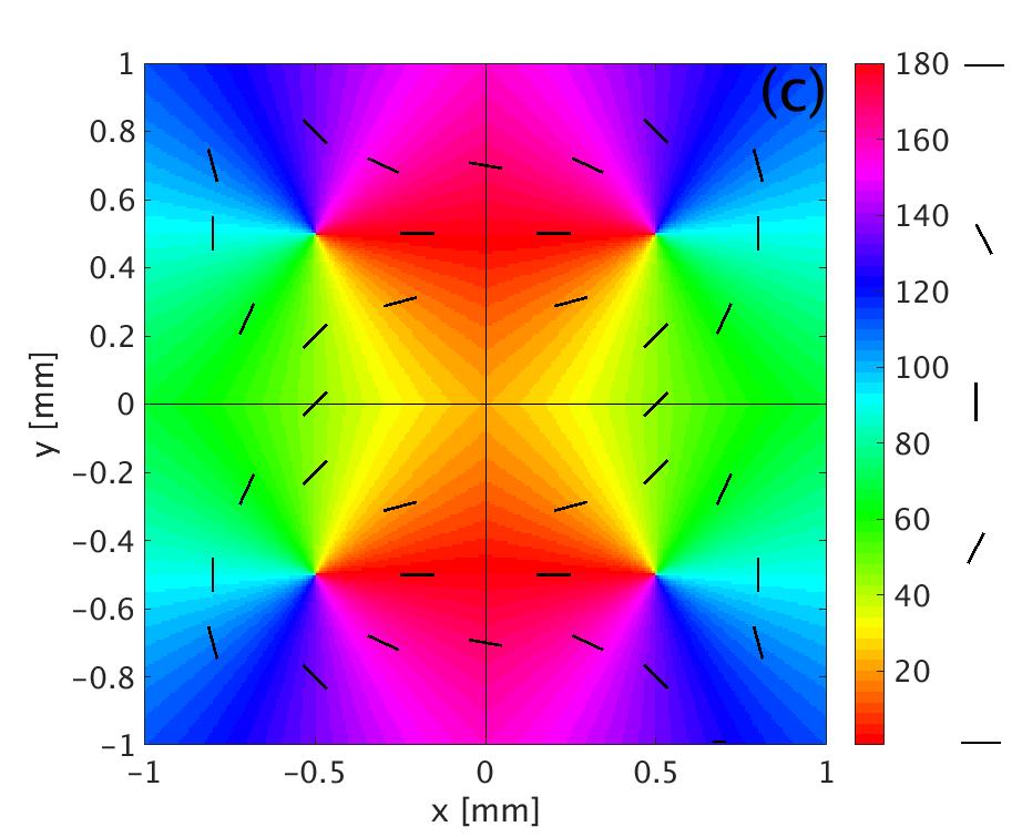
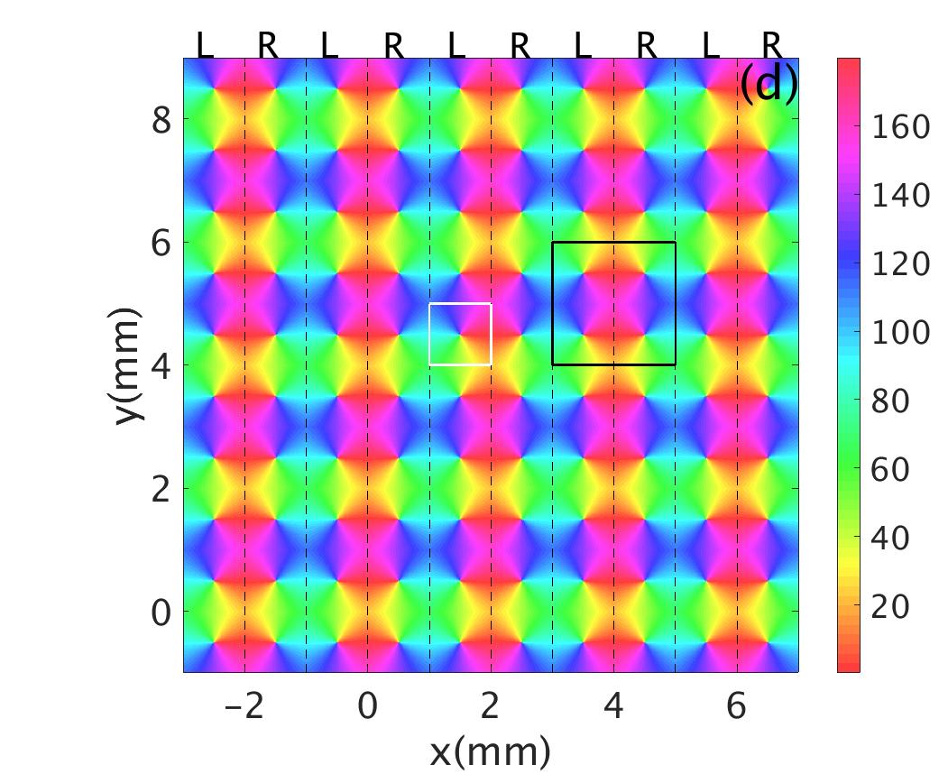
A prominent feature of V1 is the presence of ocular dominance (OD) stripes, which reflect the fact that left- and right-eye inputs are mapped to alternating stripes mm wide, with each hypercolumn including left- and right-eye OD regions. Orientation preference (OP) of neurons for particular edge orientations in a visual field is mapped to regions within each hypercolumn such that neurons with particular OP are located adjacent to one another and OP spans the range from to . Typically, OP varies with azimuth relative to a center, or singularity, in the hypercolumn in an arrangement called a pinwheel. The OP angle in each pinwheel rotates either clockwise (negative pinwheel) or counterclockwise (positive pinwheel), and neighboring pinwheels have opposite signs (Blasdel, 1992; Braitenberg and Braitenberg, 1979; Götz, 1987, 1988; Swindale, 1996). Hence, a hypercolumn must have left and right OD stripes with positive and negative pinwheels in each, as suggested by Bressloff and Cowan (2002) and Veltz et al. (2015). In Figs 1(a) and (b) we illustrate a negative pinwheel and a positive pinwheel, respectively, while Figs 1(c) and (d) show a hypercolumn containing four pinwheels, and an array of such hypercolumns, respectively. In such an array, the hypercolumn is the unit cell of the lattice and the schematic resembles maps reconstructed from in-vivo experiments, although the stripes have been approximated as straight here (Blasdel, 1992; Bonhoeffer and Grinvald, 1991, 1993; Obermayer and Blasdel, 1993).

An additional feature of V1 is that regions of similar OP are preferentially linked within and between unit cells by patchy lateral connections (Gilbert and Wiesel, 1983; Rockland and Lund, 1982). Furthermore, patchy connections into and out of a given OP region are concentrated along an axis that points in the direction of the OP. This means that cells that are sensitive to a contour of given orientation preferentially project to (and receive projections from) cells of similar OP located along the continuation of that contour, which has been argued to be important to the completion of occluded contours and the binding problem (Miikkulainen et al., 2005; Stemmler et al., 1995; Loffler, 2008; Li, 1998). Most notably, the projections from a given unit cell depend strongly on the OP at the source neurons within that cell and are thus strongly anisotropic (Bosking et al., 1997).
When one considers activity in V1, numerous experiments and studies (Eckhorn et al., 1988; König et al., 1995; Singer and Gray, 1995; Engel et al., 1990; Hata et al., 1991; Gray et al., 1989) have shown that neurons with similar feature preference in V1 exhibit synchronized gamma band (30 – 70 Hz) oscillations when the stimulus is optimal, by measuring the multi-unit activities (MUA) and local field potentials (LFP) in area 17 of cats using multi-electrodes. They also showed that the corresponding two-point correlation functions of MUA or LFP commonly have peaks at zero time-lag. Moreover, these synchronized gamma oscillation in V1 arise from the spatial structure of V1, modulated by the specific feature preferences involved. It also has been argued that such synchronized oscillation in gamma band may be involved in visual perception, the binding of related features into unified percepts, and the occurrence of visual hallucinations (Gray et al., 1990; Engel et al., 2001; Bressloff et al., 2002; Siegel et al., 2011; Henke et al., 2014).
Previous theoretical studies (Robinson, 2005, 2006, 2007) used neural field theory (NFT) with patchy propagators to show that patchy connectivity could support gamma oscillations with correlation properties whose features resembled those of some of the experiments noted above. However, the effect of OP on the patchy propagators was not incorporated and the correlations were only explored as functions of one spatial dimension.
In this paper, we generalize and explore the spatiotemporal correlation functions of Robinson (2006, 2007) to two spatial dimensions, and account for the effect of OP on the patchy propagators. We then compare the resulting spatiotemporal correlations with several MUA experiments. In Sec. 2, we briefly describe the relevant aspects of NFT including patchy propagators. In Sec. 3, we derive the general 2D correlation function in V1 via the linear NFT transfer function of V1. Section 4 describes a spatial propagator, which modulates the connection strength between cortical locations that have similar feature preference, and the Fourier coefficients of this propagator are applied to the numerical calculation of the correlation properties. The properties of these correlation functions are explored in Sec. 5, including their predictions for oscillation frequency, time decay, effects of the spatial separation between the measurement points, and the modulation by the OP in V1. The predictions compared with specific experimental outcomes in Sec. 6, and the results are summarized and discussed in Sec. 7.
2 Theory
In order to analyze correlations in the patchily connected cortex, we first briefly review an established neural field model of the relevant corticothalamic system in Sec. 2.1, and calculation of its approximate transfer function in the gamma frequency range of several tens of Hz, with further details of the derivations available in prior papers (Robinson, 2006, 2007). In Secs 3 and 4 we generalize the patchy connectivity to two dimensions (2D) and calculate the resulting 2D correlation functions in order to treat the effects of both OD and OP together.
2.1 Neural Field Theory
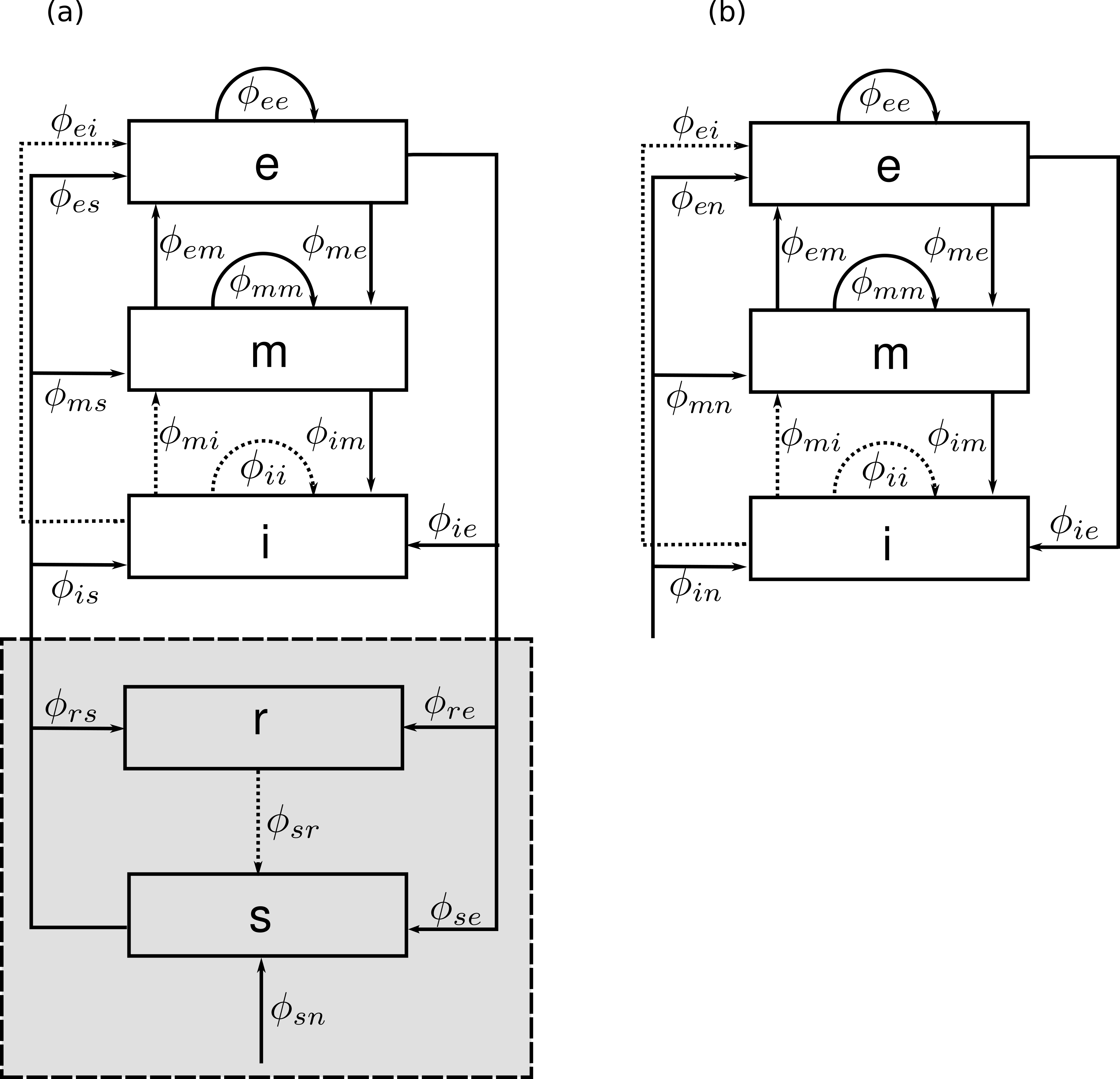
The previously developed corticothalamic model (Robinson, 2005) treats five neural populations, which are the long-range excitatory pyramidal neurons (e), midrange patchy excitatory neurons (m), short-range inhibitory interneurons (i), thalamic reticular neurons (r), and thalamic relay neurons (s); hence, it is termed the EMIRS model. Figure 2(a) shows the full EMIRS model and its connectivities between neural populations, including the axonal fields (described further below) of spike rates arriving at neurons of population from those of population , where . The external input signal is incident on the relay nuclei.
In this work, we are mainly concerned with cortical neural activities in the gamma band ( – ), which are higher than the resonant frequency () of the corticothalamic loops. This enables us to neglect the corticothalamic feedback loops of the full EMIRS model, leading to the reduced model in Fig. 2(b). This model only includes the cortical excitatory, mid-range, and short-range inhibitory populations, and the signals from the thalamus are treated as the input to the cortex. Thus, rather than having feedback inputs from the thalamus, we approximate these inputs as a common external input to the cortex. The subscript denotes the three cortical neural populations (e, m, i).
Normal brain activity has been widely modeled as corresponding approximately to linear perturbations from a fixed point, with successful applications to experiments such as electroencephalographic (EEG) spectra, evoked response potentials, visual hallucinations, and other phenomena (Henke et al., 2014; Robinson et al., 1998, 2002, 2004). Hence, in the present work, we restrict attention to the linear regime, which is justified so long as stimuli are not too strong.
NFT averages neural properties and activity over a linear scale of a few tenths of a millimeter to treat the dynamics on larger scales, which is appropriate for the present applications (Deco et al., 2008; Robinson et al., 2005).
Cells with voltage-gated ion channels produce action potentials when the soma potential exceeds a threshold . In the linear regime, changes in the mean population firing rate are related to the mean soma potential by
| (1) |
where is a constant.
The mean linear perturbation to the soma potential of neurons is approximated by summing contributions that resulting from activities of all types of synapse on neurons in the spatially extended population from those of type . Thus,
| (2) |
where is the spatial location on the cortex, approximated as a 2D sheet, and is the time. In the Fourier domain, Eq. (2) can be written as
| (3) |
where we define the Fourier transform and its inverse via
| (4) |
| (5) |
Due to the dependence of on the synaptic dynamics, signal dispersion in the dendrites, and soma charging, the soma potential corresponding to a delta function input can be approximated by
| (6) |
where is the arrival rate of incoming spikes, and is the synapse-to-soma transfer function, with
| (7) |
where and are the decay and rise rates of the soma response, respectively.
In Eq. (6), depends on at various source locations and earlier times (Robinson, 2007), whose influences propagate to from via axons, with
| (8) |
| (9) |
where describes axonal propagation. In Eq. (9), is the time delay between spatially discrete neuron populations (i.e., not between different r on the cortex) and represents the coupling of to population . In the simplest case of proportional coupling,
| (10) |
where is the mean number of synaptic connections to each neuron of type from neurons of type and is their mean strength. More generally, can describe couplings that are sensitive to other features of , such as spatial or temporal derivatives, which can increase sensitivity to features such as edges in the visual stimulus (Robinson, 2005, 2006, 2007).
Axonal propagation can be approximately described by a damped wave equation (Jirsa and Haken, 1996; Robinson et al., 1997; Schiff et al., 2007)
| (11) |
where is the temporal damping coefficient, is the wave velocity, and is the characteristic range of axons that project to population from . In Fourier space, in the absence of patchy connections, one has (Robinson, 2005)
| (12) |
| (13) |
To incorporate the patchy propagation, we approximate the OP-OD structure of V1 as being periodic, which results in periodic spatial modulation of the propagator in Eq. (9), giving (Robinson, 2007)
| (14) |
where the are the Fourier coefficients of the function that describes the spatial feature preference (i.e., OP and/or OD), and ranges over the reciprocal lattice vectors of the periodic structure (Robinson, 2007). We analyze the in Sec. 4 below.
2.2 System Transfer Function and Resonances
Turning to the system in Fig. 1, Eqs (15) – (17) can be used to write the activity changes in the pyramidal neurons in terms of changes in the firing rate that implicitly drives the input signal . At gamma frequencies, where corticothalamic feedback is too slow to respond effectively, this was found to yield (Robinson, 2006, 2007)
| (18) |
Resonances of the system that determine spatiotemporal properties of the gamma oscillations arise from the poles of the transfer function, which correspond to zeros of the denominator of Eq. (18). At millimeter scales, and , so the resonance condition becomes
| (19) |
Substituting Eqs (7), (12), (16), and (17) into Eq. (19) gives
| (20) |
where
| (21) |
When , the denominator on the left hand side of Eq. (20) is small, and the corresponding term dominates the sum over the lattice vectors . Assuming is purely spatial, can be written as , so Eq. (20) becomes (Robinson, 2006, 2007)
| (22) |
| (23) | ||||
Robinson (2007) showed that each value of can yield a resonance with frequency
| (24) |
if is sufficiently large and negative. Waves at these combinations of K and dominate gamma activity.
2.3 Transfer Function Due to Resonances
The correlation analysis of Robinson (2007) approximated the transfer function using only the lowest reciprocal lattice vector . We generalize that result to include higher order lattice vectors that describe finer spatial structure of the OP map, and denote the corresponding frequencies as . Then, the transfer function is
| (25) |
| (26) |
| (27) |
where is defined in Eq. (17). Spatially Fourier transforming Eq. (25) then gives
| (28) |
where is a modified Bessel function of the second kind (Olver et al., 2010).
3 Correlation Functions
This section summarizes the use of transfer functions to derive the two-point correlation function between the cortical firing rates measured at two different locations, when the cortex is stimulated at two locations, generalizing the analysis of Robinson (2007) and improving its notation.
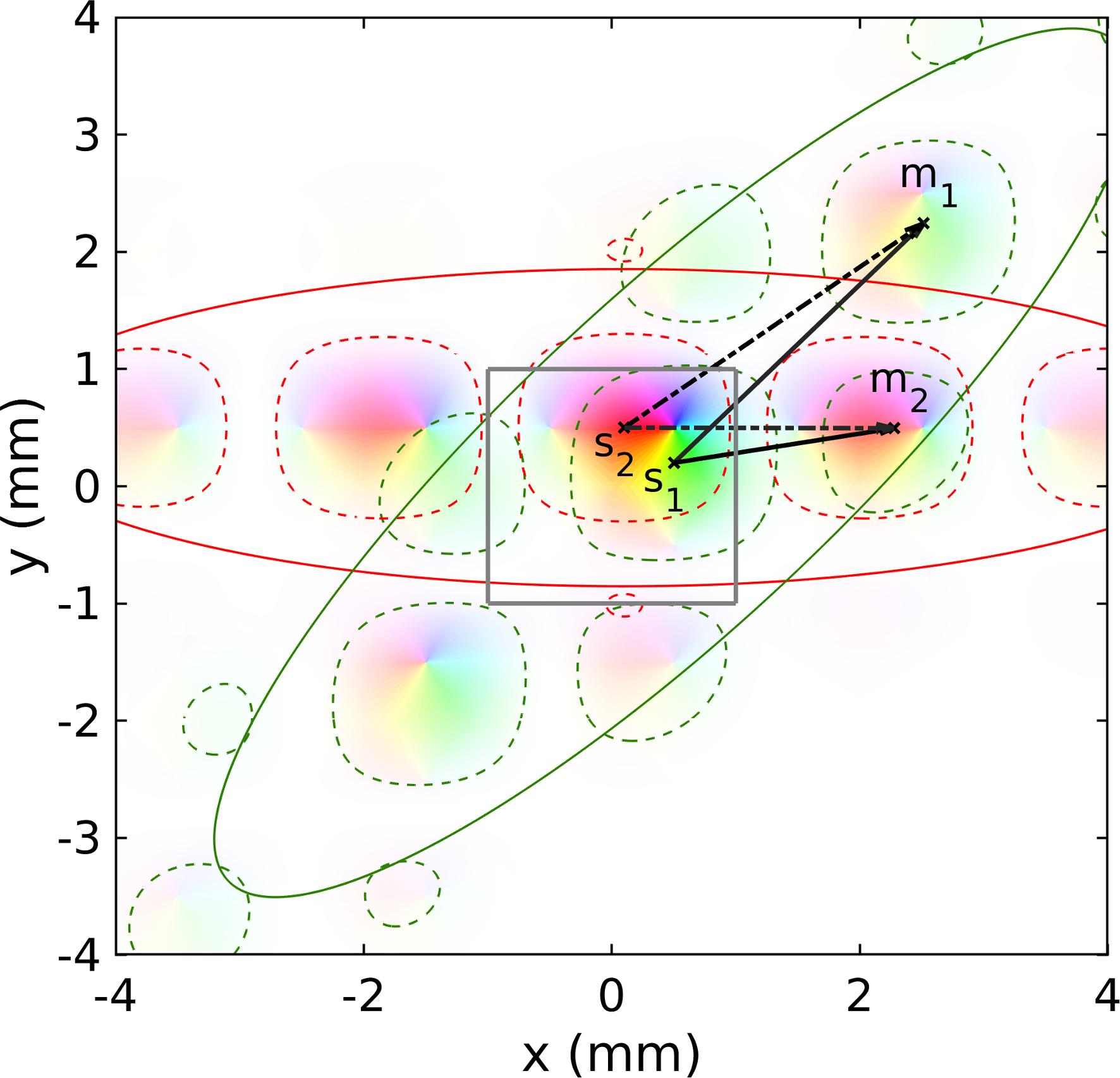
If the visual cortex receives two uncorrelated and spatially localized inputs at locations and . Further, cortical activity is measured at and . Figure 3 shows a schematic of typical spatial locations and OPs involved in deriving the correlation function. The two ellipses in solid green and red, centered at and represent anisotropic propagators for OPs and . The arrows indicate propagation of neural activity from sources to measurement points .
We first derive equations for the neural activities at and due to inputs at and . The activity at can be written as
| (29) |
where is the transfer function that relates the activities at and time to the stimulus at and time .
Robinson (2007) approximated a spatially localized input as
| (30) |
whence
| (31) |
where the real quantities and are the amplitude and the phase of the input at . We then find
| (32) |
The two-point correlation function between and is (Robinson, 2007)
| (33) |
where , and the angle brackets refer to the averages over and over the phase of the inputs. A Fourier transform and integration over achieves the averaging Robinson (2007) to yield
| (35) |
Substituting Eq. (32) into Eq. (3), and taking the inverse Fourier transform then gives
| (36) | |||||
where the angle brackets now denote the average over the phases at and . If the phases of the inputs are random and uncorrelated,
| (37) |
so the cross terms between and in Eq. (36) are zero and
| (38) | |||||
which is the sum of the correlations due to the two stimuli taken separately.
Finally, substituting Eq. (28) into Eq. (38), assuming inputs at different are uncorrelated, and letting for simplicity, gives
| (39) | |||||
Some general aspects of Eq. (39) are that the correlations fall off on a characteristic spatial scale of because at large in the right half plane. For the same reason, there is an oscillation with spatial frequency of , while resonances in select dominant temporal frequencies in the correlations.
4 Patchy Propagation
Robinson (2007)showed that the gamma response can be approximated as a sum of resonant responses at various . He further analyzed a spatially 1D system by approximating the contributions of these poles as Gaussians in space. This yielded patchy propagation with a Gaussian envelope as a function of distance, which explained a number of gamma correlation properties.
Here we generalize the analysis of Robinson (2007) to the spatially 2D cortex and to allow for the spatial anisotropy of the envelope of patchy connections, which extend furthest along a direction corresponding to the orientation of the source OP. We quantify the patchy propagation via the coefficients in Eq. (14). Robinson (2007) previously approximated the spatial propagator in 1D as a Gaussian function. The propagation was assumed to be isotropic with its patchiness described as , from which is formed by a pair of complex conjugated coefficients and , is the lowest reciprocal lattice vector. However, in 2D, patches of neurons with similar feature preference are preferentially connected, with connections (Bressloff and Cowan, 2003; Gilbert and Wiesel, 1983; Lund et al., 2003; Muir et al., 2011), concentrated toward an axis corresponding to their OP angle (Bosking et al., 1997; Malach et al., 1993; Sincich and Blasdel, 2001). To model this overall modulation of the anisotropic propagation, we approximate the spatial propagator at each point and Fourier transform it to obtain a set of coefficients , where corresponding to the reciprocal lattice vectors. These coefficients are used to calculate the transfer function described by Eqs (26) and (28).
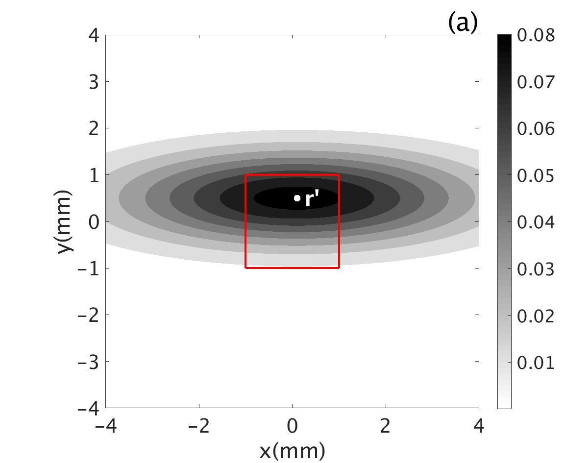
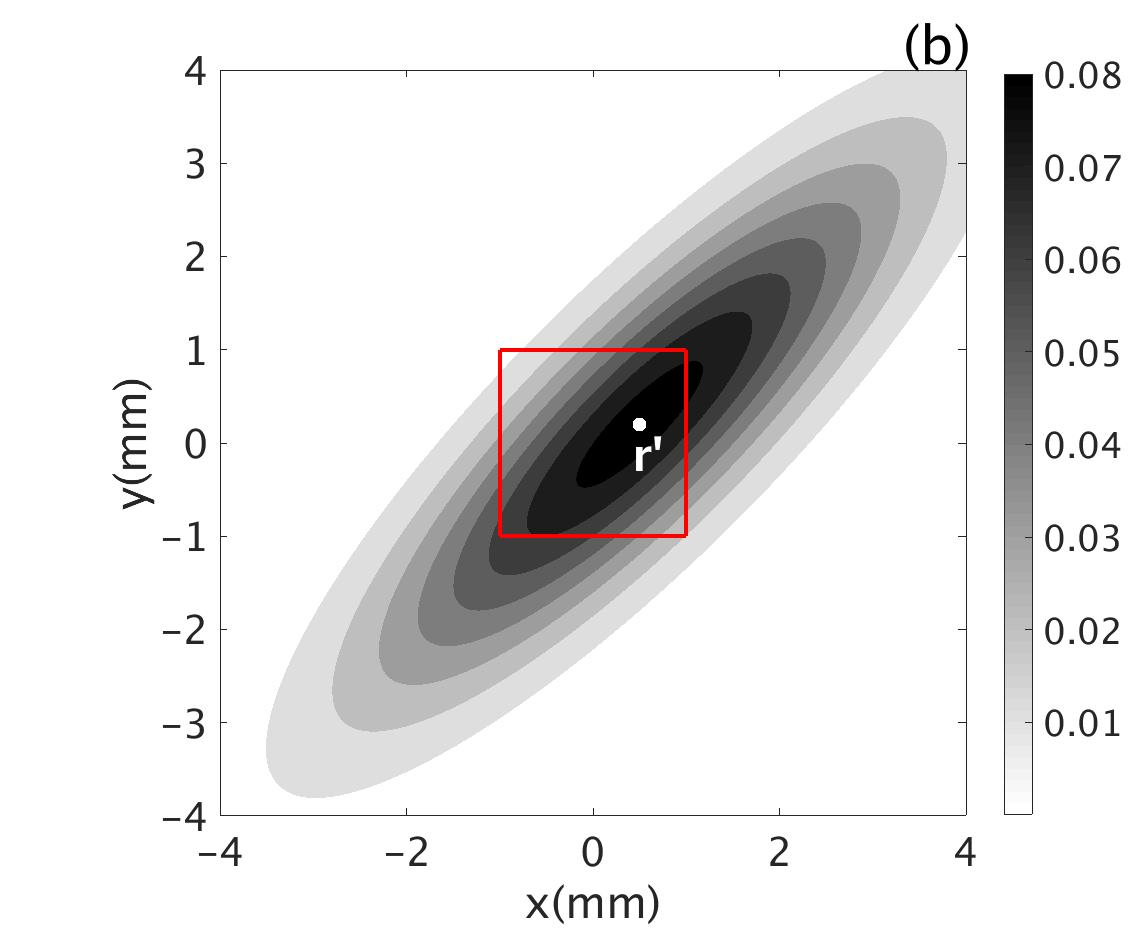
A reasonable approximation to the envelope of the patchy connections that emerge from a particular point is an elliptic Gaussian whose long axis is oriented at the local OP at . If and , we have
| (40) |
where
| (41) |
| (42) |
where and are the spatial ranges along the preferred and orthogonal directions, with values chosen to match the experimental findings in tree shrew by Bosking et al. (1997). Figures 4(a) and (b) show contour plots of for OPs of 0∘ and 45∘, respectively and source points within a central unit cell [see Fig. 1(c)].
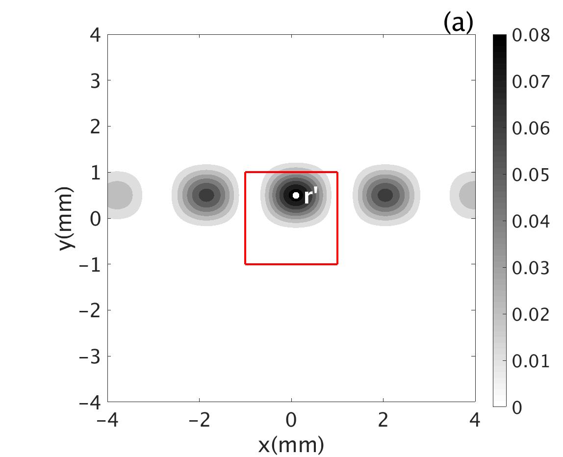
Patchy propagation is modulated with spatial period parallel and orthogonal to OD columns, where 2 mm is the width of the unit cell. To incorporate this modulation, we multiply the oriented elliptic Gaussian function by a product of cosine functions that reflect this periodicity. This gives an approximate propagator profile of the form
| (43) | |||||
where . We use this functional form to generalize the 1D cosine-modulated Gaussian form of Robinson (2007) to represent the propagator of a given resonance in the 2D anisotropic case. Figures 5 (a) and (b) show the resulting propagators for , with and . For both cases, when the underlying neurons respond to the stimulus, regardless of OP.
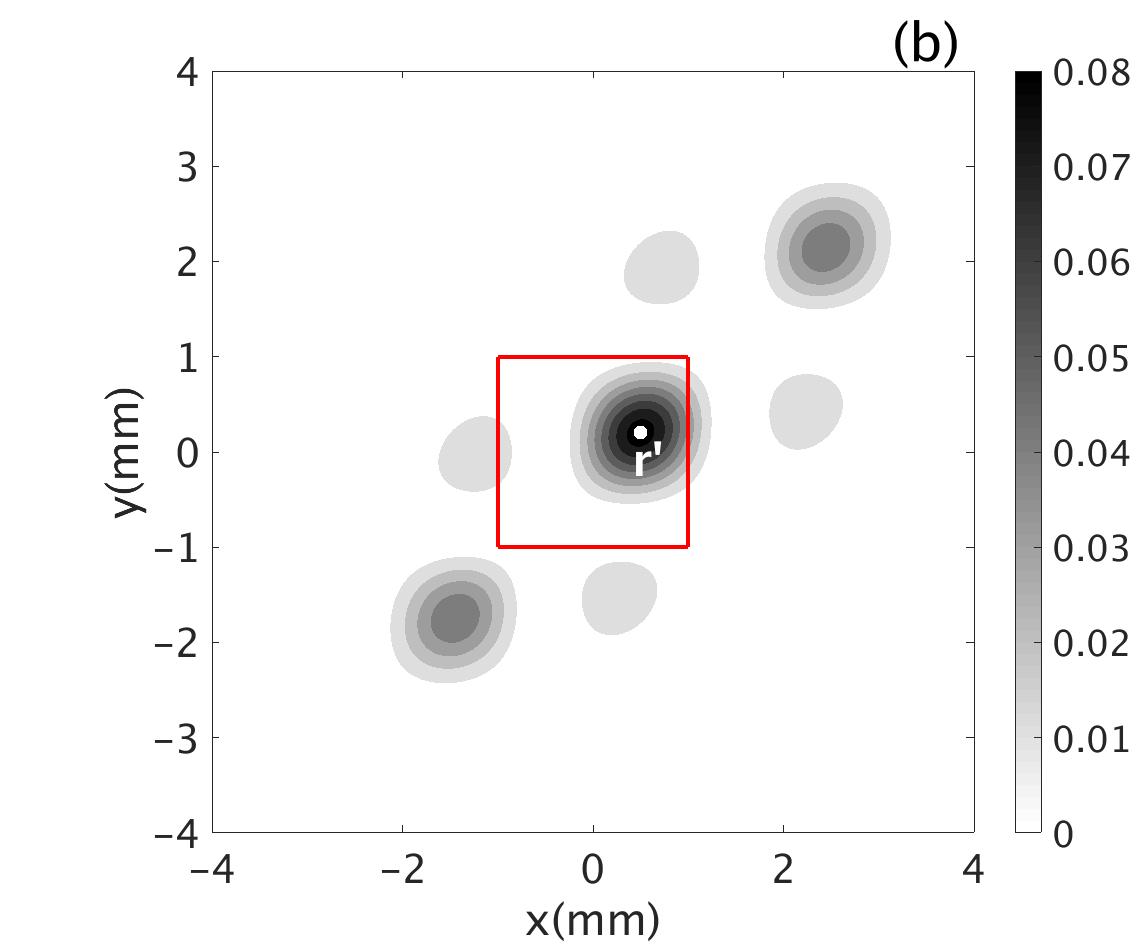
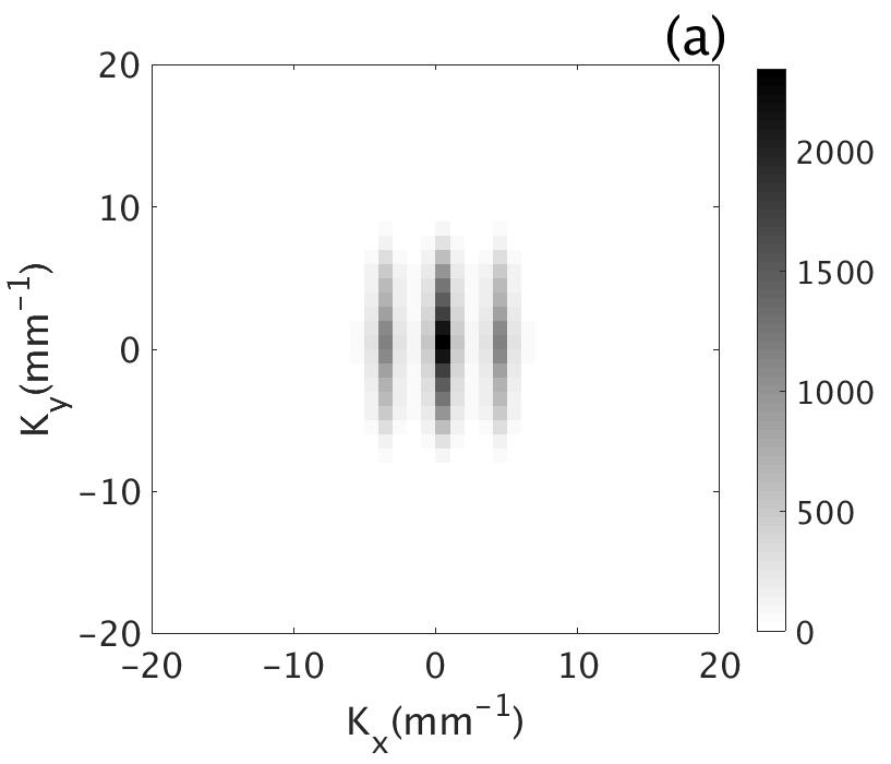
After performing a 2D Fourier transform on the propagators shown in Figure 5, the coefficients are illustrated in Figure 6 . Both two sets of coefficients do not have high frequency components. In later section, we choose a fraction of , which preserves the basic spatial propagation structure, for evaluating the transfer function.

5 Spatiotemporal properties of the correlation function
Here, we first explore the temporal properties of the correlation function in Eq. (39). Then we explore its spatial properties with a single input. Lastly, we examine the spatial correlation in the case of two input sources.
In all the cases described below, the correlation is calculated by numerically evaluating Eq. (39) and locating , , , and under different conditions. These conditions include using different optimal OPs for the measurement points and source points, and varying the distances between the measurement points. The results are presented in Fig. 7. All correlations are normalized such that when , and are placed very close to the sources. Table 1 summarizes the parameters we use for the calculations.
| Synaptodendritic rates | , , | 80 | s-1 |
| , , | s-1 | ||
| Projection Range | mm | ||
| mm | |||
| mm | |||
| Damping rates | s-1 | ||
| s-1 | |||
| Gains | |||
| s-1 |
5.1 Temporal Correlation Properties
In Fig. 7(a), we illustrate the temporal correlations evoked by binocular stimulation when and have the same OP and and are located in the same unit cell, but in different OD columns. The strength of propagation of neural signals from two sources is indicated by contour lines of Eq. (43); the propagation is predominantly parallel in this case.
The points and are located in a different unit cell to the source points; are approximately away from each other; and are located at approximately from their respective collinear source points, the OPs at and are also . We have also placed additional measurement points and , with the same OP as and , but are approximately from the sources.
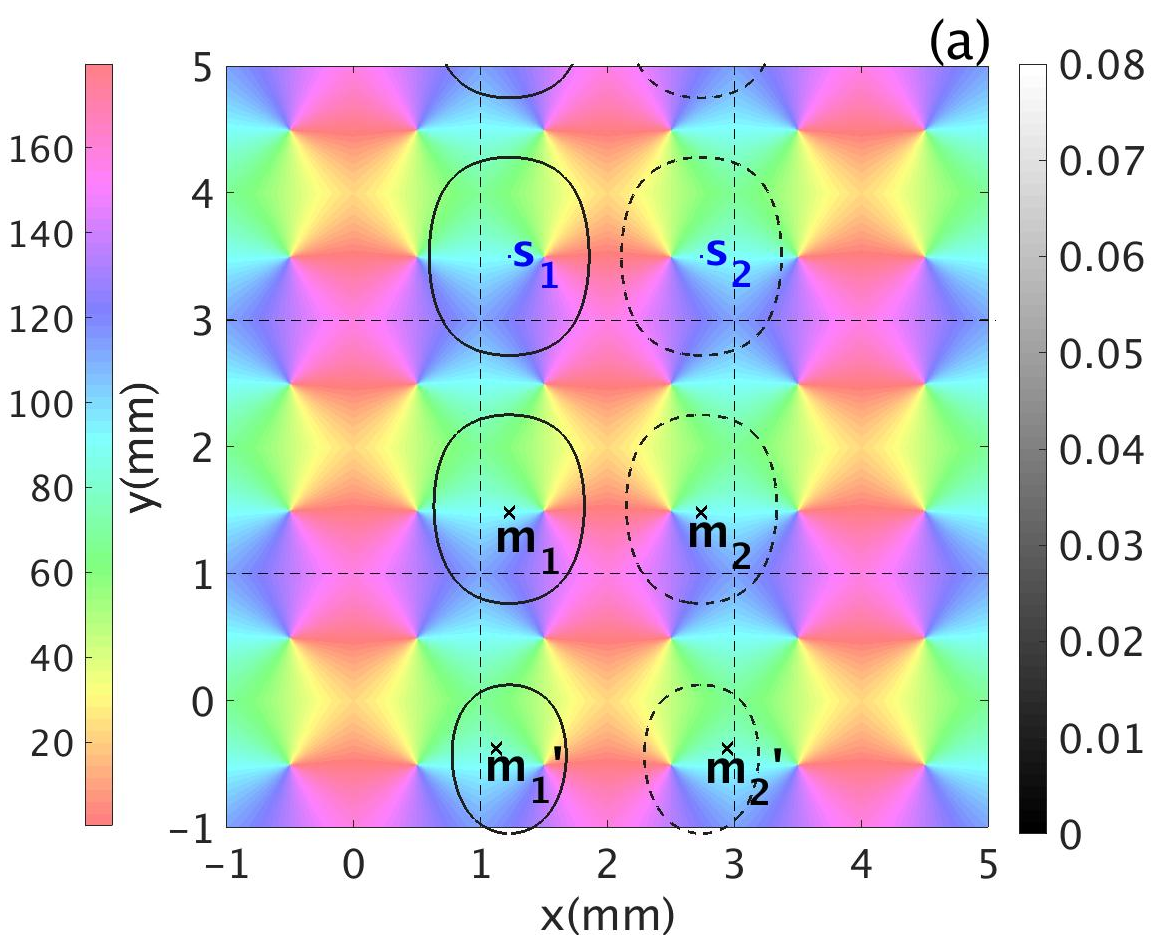
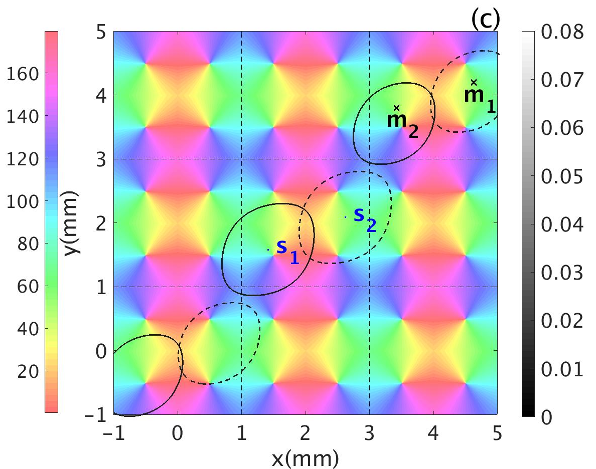
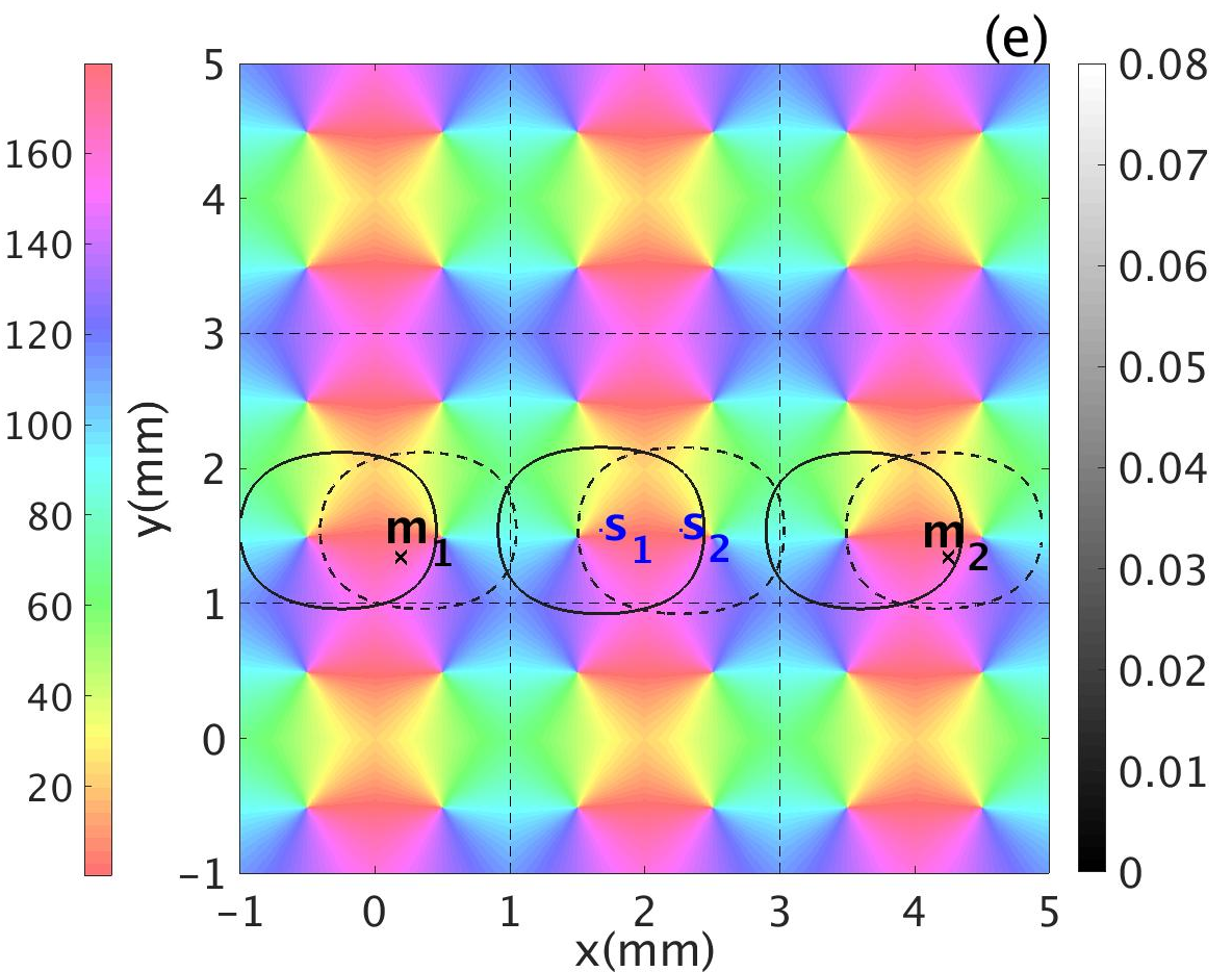
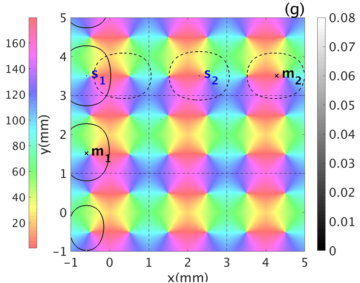
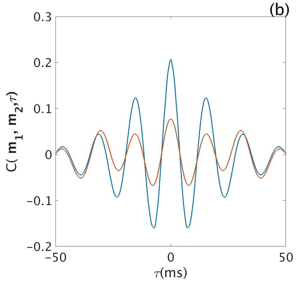
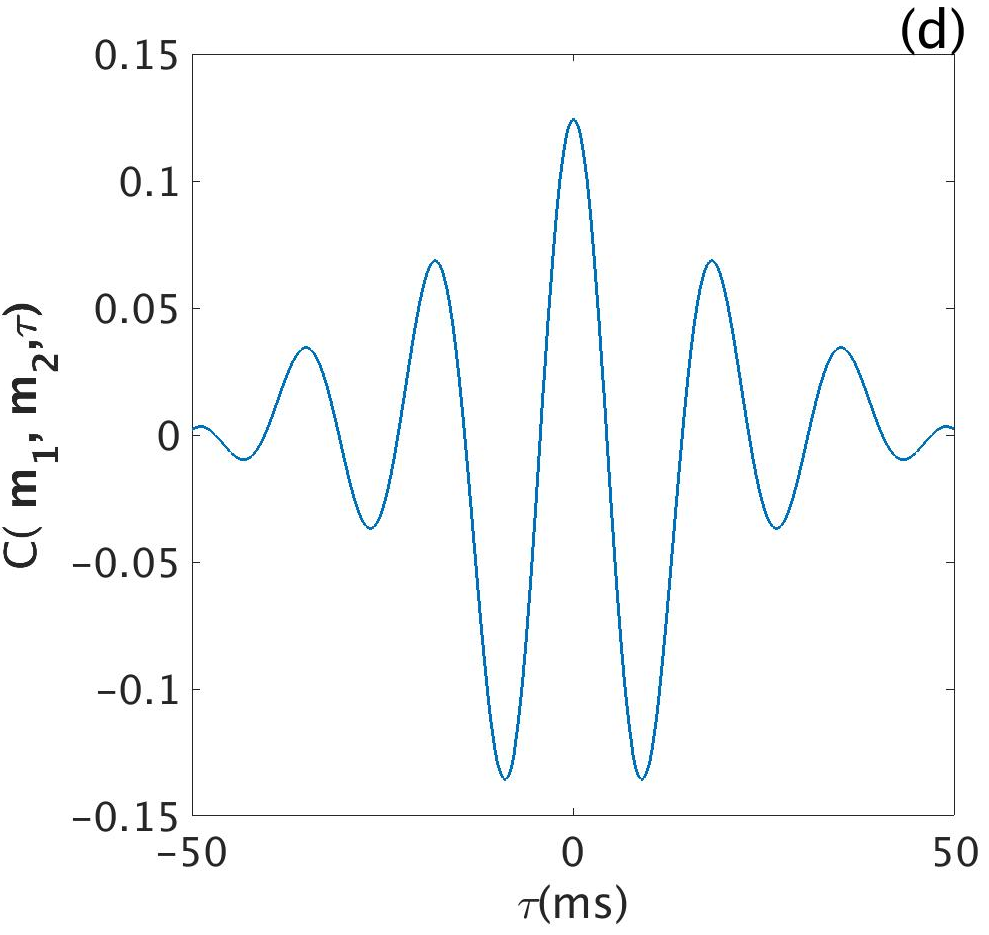
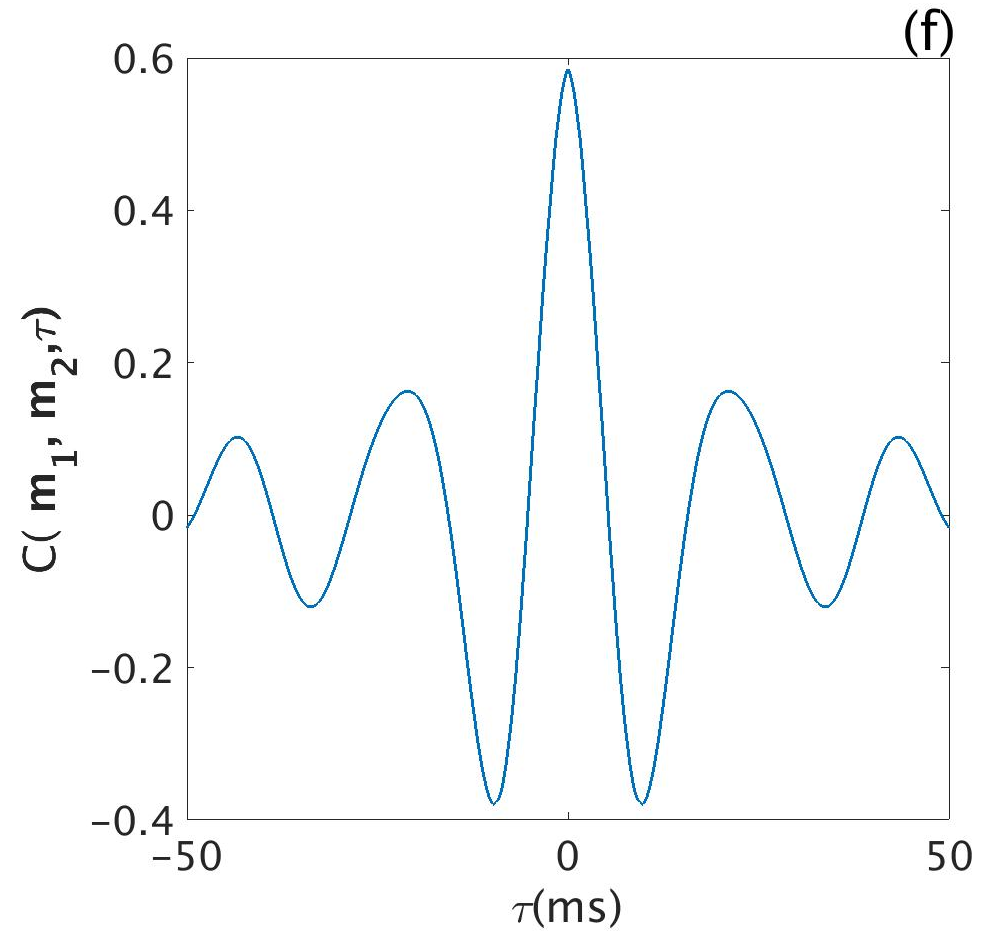
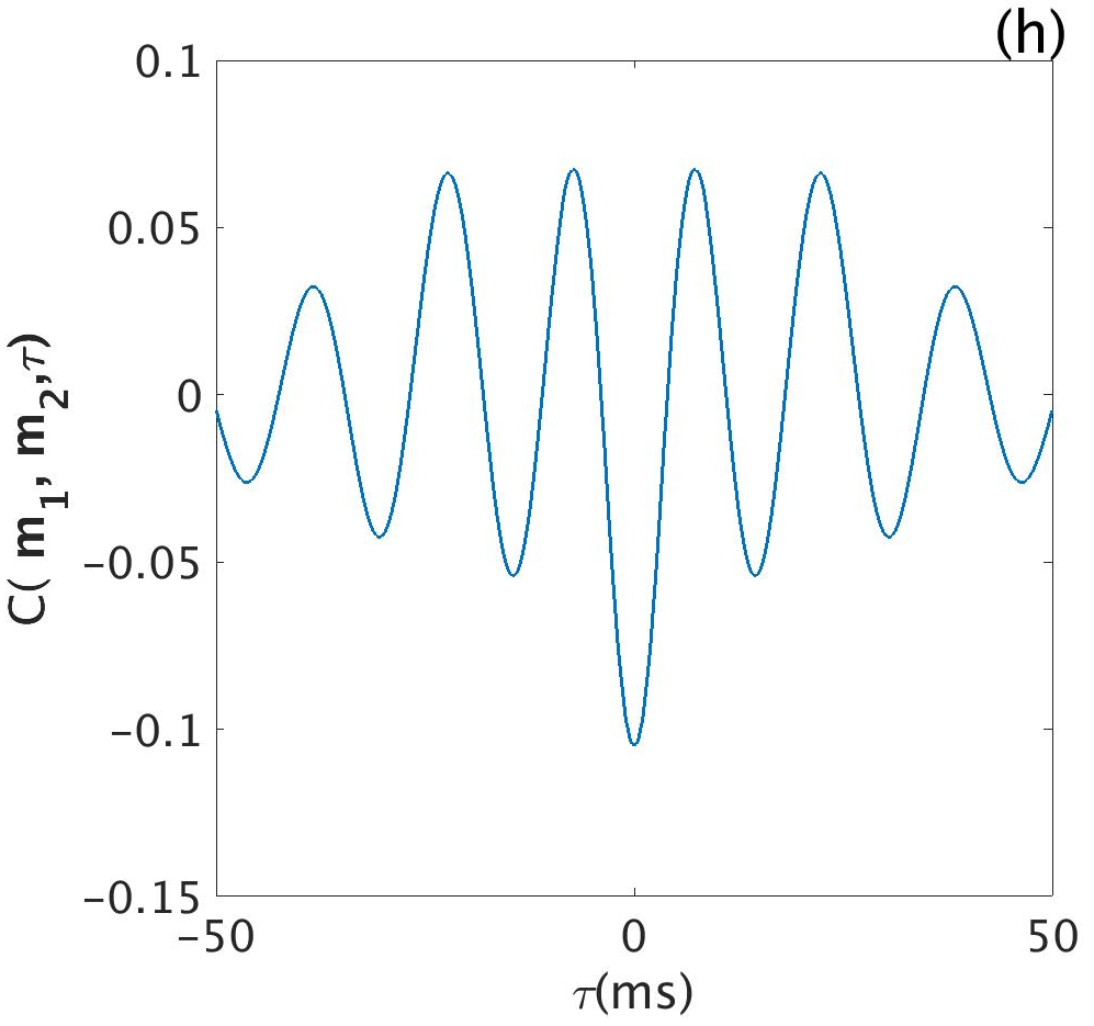
Figure 7(b) shows the temporal correlation functions and . Both oscillate at around , in the gamma range. Furthermore, each has a peak centered at , so the neural activities at and , and , are synchronized. The time for their envelopes to decrease to () of the peak value is . However, when the measurement points are placed further away from the sources, the correlation at becomes weaker, as seen by comparing the two curves.
Figure 7(c) shows a case for which the OP of all sources and measurement points is equal (at ). Figure 7(d) shows that the resulting correlation also has a central peak at zero time-lag, oscillates in the gamma band at , and its envelope decreases by at .
In order to explore the correlation properties between OD columns, we place all the source points and measurement points co-linearly with OP in Figure 7(e). Synchronized activities at and are shown by the center peak at in Fig. 7(f). This correlation also exhibits gamma band oscillation at , and the decrease by from the peak happens at . One thing worth to be mentioned here is that the correlation strength due to inter-columnar connection shown in Fig. 7(f), is stronger than the intra-column connection in Fig. 7(b).
To further investigate the correlation properties, Fig. 7(g) shows a case in which the two measurement sites have orthogonal OPs, and so does the sources: the OP at and is , while at and it is . The distance between the two measurement points is around . In this case, tends to evoke strong response at , but not at . This introduces an anticorrelation between and . Similarly, adding another source only stimulates and it again makes the activities at two measurement sites anticorrelated. This negative correlation is exactly shown by our predicted result in Fig. 7(g). It displays a negative peak at .
5.2 Two dimensional correlations due to a single source
To demonstrate how the correlation strength is influenced by the location of the measurement sites and their OP, we fix the location of a source and a measurement point , as in Fig. 7(a). We then map the correlation with the second measurement point at as a function of the latter’s position on V1. The resulting map is shown in Fig. 8, normalized to the maximum value of .
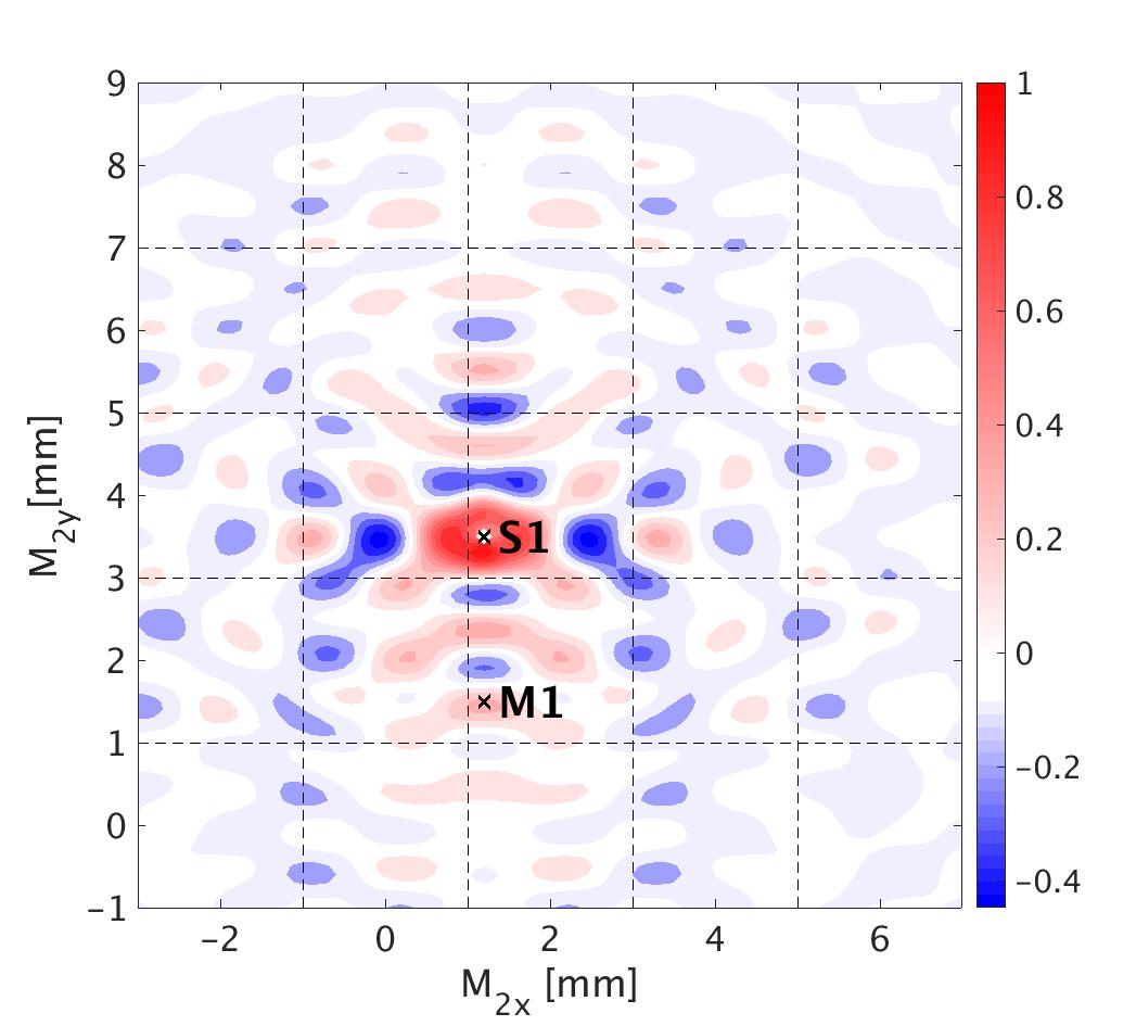
Figure 8 shows that: (i) The strongest positive correlations are located along a vertical axis passing through the source point whose OP is ; (ii) Patterns of the correlated regions are almost symmetric around the vertical axis in (i); (iii) The correlation strength falls off with distance between the two measurement points, as expected from Eq. (43); In addition, the correlation nearly vanishes when the measurement sites are greater than apart, and this agrees with the experimental results, which suggested that oscillatory cross-correlations are not observed when the spatial separation of neurons exceeds . (iv) The central peak shows that when the distance between and is less than , the correlations are strong and do not depend on the OPs at these locations, in accord with experiments (Bosking et al., 1997; Engel et al., 1990; Gray et al., 1989; Swindale, 1996). (v) The positive correlations correspond to regions of OP approximately equal to ’s OP. while negative correlation regions correspond to OPs approximately perpendicular to the source OP angle. This shows that only neurons with similar OP to the source respond to the input stimulus.
5.3 Two dimensional correlations due to two sources
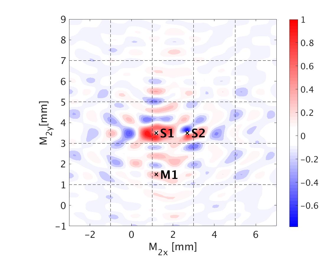
Here we explore the dependence of the correlation function on the position of measurement point with two inputs and . The location of the measurement points and source points are set up exactly as in the previous case and the additional source has the same OP as (i.e. ).
The resulting map is shown in Fig. 9 and has similar properties to the previous case with one input, namely, the strongest correlations between the measurements points are along a vertical axis, which matches the OP of the sources. The positive correlation regions along this axis have a spatial period of , corresponding to the minimum distance between regions having the same OP angle as the sources. However, the negative correlation regions now tend to align horizontally, which represents the direction orthogonal to the OP. The input source is not surrounded by positive correlation regions as is; rather, the negative correlations right above correspond to a region where the OP of is . This is consistent with Sec. 5.1, where we showed that measurement points with orthogonal OPs tend to be anticorrelated at . In that case, we have predicted that when the OP of two measurement points are and respectively, the source that is optimal to one of the measurement site introduces negative correlation between the two.
6 Comparison Between Theory and Experiment
In this section, we compare the predicted correlation functions with experimental correlations obtained from Engel et al. (1990), who published temporal correlation functions of MUA and LFP data under various conditions.
6.1 Description of the Experiments
In these experiments, the MUA and LFP measurements were recorded from an array of electrodes that were inserted in 5 to 7 spatially separated sites in area 17 of anesthetized adult cats, with neighboring recording sites spaced 400 – 500 m apart. Oriented light bars were used as binocular stimulation. Each trial lasted for 10 seconds and one trial set was composed of 10 trials with identical stimuli. During each trial, the light bars were projected onto a screen that was placed in front of the eye-plane of the cat. The autocorrelation function (ACF) and cross-correlation function (CCF) of the MUA data were computed. CCFs were calculated on each individual trials first, then averaged to get the final single CCF corresponding to a specific input stimulus Engel et al. (1990).
6.2 Mapping experimental conditions to a regular lattice
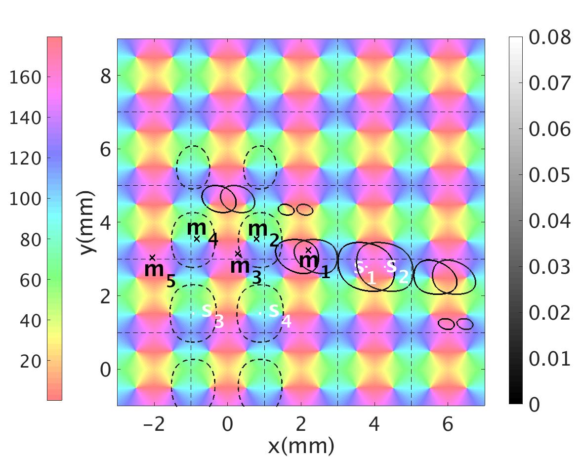
The experimental stimulation was binocular, so a single moving light bar at a specific point in time, maps to two source points on V1 ( and ), both with OP equal to the bar orientation, one located in left OD column and one in the right OD column.
In Engel et al.’s experiments, there are five fixed measurement points labeled as to . Cells at measurement points , , and have similar orientation preference and are nearly orthogonal to the OP preference of cells at measurement points , . We map these points onto the regular grid used in our model, which results in slight distortion ( mm) of the original cortical surface in order to preserve the measurement-point OPs. The OPs of to , computed after mapping onto our regular lattice match to the OPs given by the experiments within .
Here, we calculate the temporal correlation functions for two sets of experimental conditions, where the only difference between the two is the OP of the stimulus. One stimulus is oriented at and another one oriented at . Figure 10 shows both the stimulation and measurements sites on the idealized OP map. The sources and indicate the stimulus, while and represent the the stimulus. The locations of the measurement sites to are the same for the two sets of experimental conditions.
6.3 Comparison of Predicted and Experimental Correlation Functions
According to the experimental findings in Engel et al. (1990), when the input light bar is oriented at , measurement sites , , and have synchronized oscillatory responses; and, when the input light bar is oriented at , and are stimulated simultaneously. Figure 11 shows the CCFs and ACFs calculated from the experimental data. In Figure 11(a), the synchronized activities at , , and are evoked by a oriented stimulus. All the cross correlograms are peaked at zero time-lag and have an average oscillation frequency of . The envelope of the correlograms decreases to of its center peak value at around . The ACFs and CCF of and from a vertical light bar stimulus are shown in Figure 11(b). The CCF between and oscillates at around , and it takes more than for the correlation strength to decrease to of its maximum.
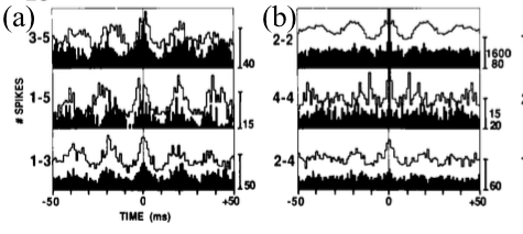
Moreover, in the experiments it was also found that the correlation strength between is weaker than that between and between (i.e., the bar that indicates the number of spikes, on the right of the plot in the second row of Figure 11(a), has smaller number than other two plots). This is due to the fact that the spatial distance between and is the largest, and the correlation strength falls off with distance.
We next explore the properties of our predicted correlation functions using Eq. (39) with the experimental conditions. Figure 12(a) shows the plots of our predicted temporal correlation functions between and , and , and and . Similarly to the experimental CCFs, all the theoretical CCFs: (i) are oscillatory and peak at zero time lag; (ii) have an oscillation frequency around ; and, (iii) have their characteristic time for the correlation envelope to decrease by of the maximum value at approximately . These theoretical results agree with the experimental results, once a nonzero mean baseline is subtracted from the latter.
Our prediction also captures the spatial dependence of the maximum correlation strength. The plot in the middle row of Figure 12(a) corresponds to the correlation between and has the smallest amplitude among the three CCFs.
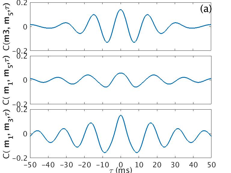
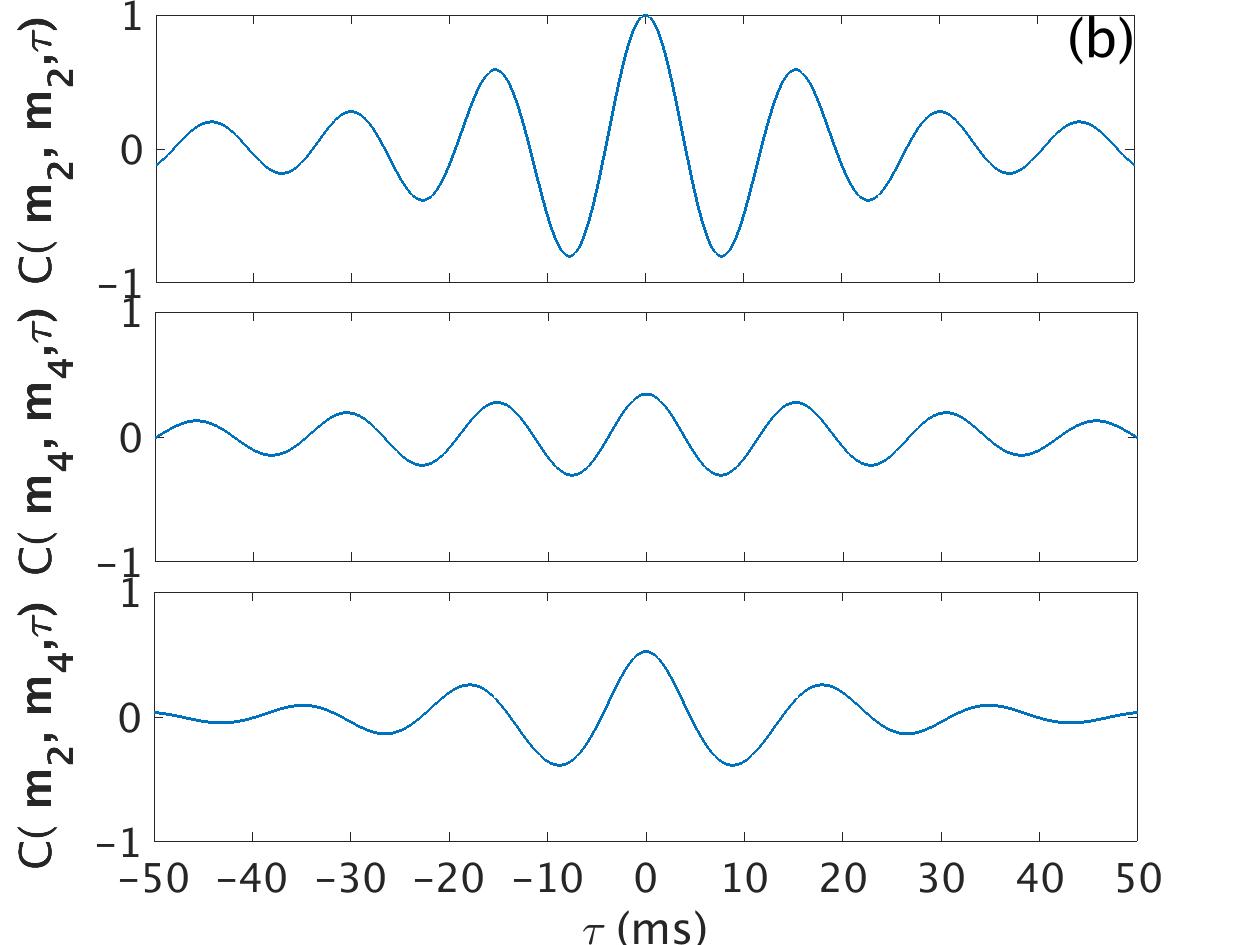
Figure 12(b) shows the predicted temporal correlation function generated by the vertical input light bar. In order to be consistent with the experimental results shown in Figure 11(b), the autocorrelation functions of and are also included in the top two rows of Figure 12(b). Both ACFs show oscillations in the gamma band. The CCF between and shows a center peak at and oscillates at . The time for the envelope decay to of the center peak value is . These properties are also in line with the experimental findings.
7 Summary and Conclusion
We have generalized the spatiotemporal correlation functions in two dimensions that incorporates the spatial structure of the OP map and OD columns of V1. Our results show that the neural activities are synchronized in gamma band when neurons have similar feature preference. The main results are:
(i) The derivation of a shape function that modulates the spatial patchy propagation of the neural signals. The shape function models the propagation such that the orientation of the propagation direction is aligned with the OP of source, and the connected neurons are patchy and periodically located. The parameters of the shape function are tuned to match the propagation ranges observed in experiments (Bosking et al., 1997).
(ii) The systematic characterization of the 2D two-point temporal correlation function. The generalized correlation function is evaluated numerically for various combinations of stimulation and measurement sites. The results demonstrate a synchronized gamma oscillation exists between two groups of neurons that have similar OP to the sources. The correlation strength is larger for inter-columnar connections than for intra-columnar connections. As the measurement points are further away from the sources, the correlation strength decreases, and is negligible when the spatial separation of the measurement points exceeds .
(iii) The construction of a 2D correlation maps. These maps show the changes expected in the peak correlation strength with respect to the variation of the OP of one of the measurement sites, and its distance to a second measurement site. The positive correlations appear as patches on an axis oriented at the OP of the source; and, negative correlations occur where the OPs of the measurement sites are orthogonal to the OP of the source.
(iv) The comparison of the predicted temporal correlations using experimental conditions. Our theoretical results are compared with the experimental findings and shows there is a close match between both in terms of the oscillation frequency and the characteristic decay time of the correlation function envelope. In addition, our CCFs also capture the spatial dependence of correlation strength, which decreases with distance between the measurement sites.
Overall, our generalized spatiotemporal correlation function reproduces the gamma band oscillations observed in V1 and relates the spatially distributed neural responses to the periodic spatial structure of OP and OD in V1. This study lays the foundation to further investigate other visual perception phenomena such as the binding problem.
Future work will focus on using a more realistic lattice of pinwheels and introduce asymmetries between the left/right OD columns to account for strabismus.
Acknowledgements
This work was supported by the Australian Research Council under Laureate Fellowship grant FL1401000025, Center of Excellence grant CE140100007, and Discovery Project grant DP170101778.
References
- Blasdel (1992) Blasdel, G. G. (1992). Orientation selectivity, preference, and continuity in monkey striate cortex. J Neurosci, 12:3139–3161.
- Bonhoeffer and Grinvald (1991) Bonhoeffer, T. and Grinvald, A. (1991). Iso-orientation domains in cat visual cortex are arranged in pinwheel-like patterns. Nature, 353:429–31.
- Bonhoeffer and Grinvald (1993) Bonhoeffer, T. and Grinvald, A. (1993). The layout of iso-orientation domains in area 18 of cat visual cortex: optical imaging reveals a pinwheel-like organization. J Neurosci, 13:4157–4180.
- Bosking et al. (1997) Bosking, W. H., Zhang, Y., Schofield, B., and Fitzpatrick, D. (1997). Orientation selectivity and the arrangement of horizontal connections in tree shrew striate cortex. J Neurosci, 17(6):2112–2127.
- Braitenberg and Braitenberg (1979) Braitenberg, V. and Braitenberg, C. (1979). Geometry of orientation columns in the visual cortex. Biol Cybern, 33(3):179–186.
- Bressloff and Cowan (2002) Bressloff, P. C. and Cowan, J. D. (2002). The visual cortex as a crystal. Physica D: Nonlinear Phenomena, 173(3):226 – 258.
- Bressloff and Cowan (2003) Bressloff, P. C. and Cowan, J. D. (2003). The functional geometry of local and horizontal connections in a model of v1. J Physiol Paris, 97(2):221–236.
- Bressloff et al. (2002) Bressloff, P. C., Cowan, J. D., Golubitsky, M., Thomas, P. J., and Wiener, M. C. (2002). What geometric visual hallucinations tell us about the visual cortex. Neural Comput, 14(3):473–491.
- Deco et al. (2008) Deco, G., Jirsa, V., Robinson, P., Breakspear, M., and Friston, K. (2008). The dynamic brain: from spiking neurons to neural masses and cortical fields. PLoS Comput Biol, 4(8).
- Eckhorn et al. (1988) Eckhorn, R., Bauer, R., Jordan, W., Brosch, M., Kruse, W., Munk, M., and Reitboeck, H. J. (1988). Coherent oscillations: A mechanism of feature linking in the visual cortex? Biol Cybern, 60(2):121–130.
- Engel et al. (2001) Engel, A. K., Fries, P., and Singer, W. (2001). Dynamic predictions: Oscillations and synchrony in top-down processing. Nat Rev Neurosci, 2(10):704–16.
- Engel et al. (1990) Engel, A. K., König, P., Gray, C. M., and Singer, W. (1990). Stimulus-dependent neuronal oscillations in cat visual cortex:inter-columnar interaction as determined by cross-correlation analysis. Eur J Neurosci, 2:588–606.
- Gilbert and Wiesel (1983) Gilbert, C. and Wiesel, T. (1983). Clustered intrinsic connections in cat visual cortex. J Neurosci, 3(5):1116–1133.
- Gray et al. (1989) Gray, C. M., Engel, A. K., König, P., and Singer, W. (1989). Oscillatory responses in cat visual cortex exhibit inter-columnar synchronization which reflects global stimulus properties. J Physiol, 338:334–337.
- Gray et al. (1990) Gray, C. M., Engel, A. K., König, P., and Singer, W. (1990). Stimulus-dependent neuronal oscillations in cat visual cortex: Receptive field properties and feature dependence. Eur J Neurosci, 2(7):607–619.
- Götz (1987) Götz, K. G. (1987). Do “d-blob” and “l-blob” hypercolumns tessellate the monkey visual cortex? Biol Cybern, 56(2):107–109.
- Götz (1988) Götz, K. G. (1988). Cortical templates for the self-organization of orientation-specific d- and l-hypercolumns in monkeys and cats. Biol Cybern, 58(4):213–223.
- Hata et al. (1991) Hata, Y., Tsumoto, T., Sato, H., and Tamura, H. (1991). Horizontal interactions between visual cortical neurones studied by cross-correlation analysis in the cat. J Physiol, 441:593–614.
- Henke et al. (2014) Henke, H., Robinson, P., Drysdale, P., and Loxley, P. (2014). Spatiotemporally varying visual hallucinations: I. corticothalamic theory. J Theor Biol, 357:200 – 209.
- Hubel and Wiesel (1962) Hubel, D. H. and Wiesel, T. N. (1962). Shape and arrangement of columns in cat’s striate cortex. J Physiol, 165(3):559–568.
- Hubel and Wiesel (1974) Hubel, D. H. and Wiesel, T. N. (1974). Sequence regularity and geometry of orientation columns in the monkey striate cortex. J Comp Neurol, 158(3):267–293.
- Jirsa and Haken (1996) Jirsa, V. K. and Haken, H. (1996). Field theory of electromagnetic brain activity. Phys Rev Lett, 77:960–963.
- Kukjin et al. (2003) Kukjin, K., Michael, S., and Haim, S. (2003). Mexican hats and pinwheels in visual cortex. Proc Natl Acad Sci USA, 100:2848–53.
- König et al. (1995) König, P., Engel, A. K., and Singer, W. (1995). Relation between oscillatory activity and long-range synchronization in cat visual cortex. Proc Natl Acad Sci USA, 92(1):290–294.
- Li (1998) Li, Z. (1998). A neural model of contour integration in the primary visual cortex. Neural Computation, 10(4):903–940.
- Loffler (2008) Loffler, G. (2008). Perception of contours and shapes: Low and intermediate stage mechanisms. Vision Research, 48(20):2106 – 2127.
- Lund et al. (2003) Lund, J. S., Angelucci, A., and Bressloff, P. C. (2003). Anatomical substrates for functional columns in macaque monkey primary visual cortex. Cereb Cortex, 13:15–24.
- Malach et al. (1993) Malach, R., Amir, Y., Harel, M., and Grinvald, A. (1993). Relationship between intrinsic connections and functional architecture revealed by optical imaging and in vivo targeted biocytin injections in primate striate cortex. Proc Natl Acad Sci USA, 90(22):10469–10473.
- Miikkulainen et al. (2005) Miikkulainen, R., Bednar, J. A., Choe, Y., and Sirosh, J. (2005). Computational Maps in the Visual Cortex. Springer-Verlag.
- Muir et al. (2011) Muir, D. R., Costa, D., M., N., Girardin, C. C., Naaman, S., Omer, D. B., Ruesch, E., Grinvald, A., and Douglas, R. J. (2011). Embedding of cortical representations by the superficial patch system. Cereb Cortex, 21.
- Obermayer and Blasdel (1993) Obermayer, K. and Blasdel, G. G. (1993). Geometry of orientation and ocular dominance columns in monkey striate cortex. J Neurosci, 13(10):4114–4129.
- Olver et al. (2010) Olver, F. W., Lozier, D., Boisvert, R., and Clark, C. (2010). NIST Handbook of Mathematical Functions. Cambridge: Cambridge University Press.
- Robinson (2005) Robinson, P. A. (2005). Propagator theory of brain dynamics. Phys Rev E, 72:011904.
- Robinson (2006) Robinson, P. A. (2006). Patchy propagators, brain dynamics, and the generation of spatially structured gamma oscillations. Phys Rev E, 73:041904.
- Robinson (2007) Robinson, P. A. (2007). Visual gamma oscillations: waves, correlations, and other phenomena, including comparison with experimental data. Biol Cybern, 97:317–335.
- Robinson et al. (2004) Robinson, P. A., Christopher J. Rennie, C. J., D. L. Rowe, D. L., and O’Connor, S. (2004). Estimation of multiscale neurophysiologic parameters by electroencephalographic means. Human brain mapping, 23 1:53–72.
- Robinson et al. (2002) Robinson, P. A., Rennie, C. J., and Rowe, D. L. (2002). Dynamics of large-scale brain activity in normal arousal states and epileptic seizures. Phys. Rev. E, 65:041924.
- Robinson et al. (2005) Robinson, P. A., Rennie, C. J., Rowe, D. L., O’Connor, S. C., and Gordon, E. (2005). Multiscale brain modelling. Philos Trans R Soc Lond B Biol Sci, 360(1457):1043–1050.
- Robinson et al. (1997) Robinson, P. A., Rennie, C. J., and Wright, J. J. (1997). Propagation and stability of waves of electrical activity in the cerebral cortex. Phys Rev E, 56:826–840.
- Robinson et al. (1998) Robinson, P. A., Rennie, C. J., Wright, J. J., and Bourke, P. D. (1998). Steady states and global dynamics of electrical activity in the cerebral cortex. Phys. Rev. E, 58:3557–3571.
- Rockland and Lund (1982) Rockland, K. and Lund, J. (1982). Widespread periodic intrinsic connections in the tree shrew visual cortex. Science, 215(4539):1532–1534.
- Schiff et al. (2007) Schiff, S. J., Huang, X., and Wu, J. (2007). Dynamical evolution of spatiotemporal patterns in mammalian middle cortex. Phys Rev Lett, 98:178102.
- Schiller and Tehovnik (2015) Schiller, P. H. and Tehovnik, E. J. (2015). Vision and the Visual System. Oxford : Oxford University Press.
- Siegel et al. (2011) Siegel, M., Engel, A. K., and Donner, T. H. (2011). Cortical network dynamics of perceptual decision-making in the human brain. Front Hum Neurosci, 5:21.
- Sincich and Blasdel (2001) Sincich, L. and Blasdel, G. (2001). Oriented axon projections in primary visual cortex of the monkey. J Neurosci, 21(12):4416–4426.
- Singer and Gray (1995) Singer, W. and Gray, C. M. (1995). Visual feature integration and the temporal correlation hypothesis. Annu Rev Neurosci, 18(1):555–586.
- Stemmler et al. (1995) Stemmler, M., Usher, M., and Niebur, E. (1995). Lateral interactions in primary visual cortex: A model bridging physiology and psychophysics. Science, 269(5232):1877–1880.
- Swindale (1996) Swindale, N. V. (1996). The development of topography in the visual cortex: A review of models. Network, 7(1):161–247.
- Tovée (1996) Tovée, M. J. (1996). An Introduction to the Visual System. Cambridge: Cambridge University Press.
- Veltz et al. (2015) Veltz, R., Chossat, P., and Faugeras, O. (2015). On the effects on cortical spontaneous activity of the symmetries of the network of pinwheels in visual area v1. J Math Neurosci, 5(1):11.