Gaussian multipartite quantum discord from classical mutual information

Abstract

Quantum discord is a measure of non-classical correlations, which are excess correlations inherent in quantum states that cannot be accessed by classical measurements. For multipartite states, the classically accessible correlations can be defined by the mutual information of the multipartite measurement outcomes. In general the quantum discord of an arbitrary quantum state involves an optimisation of over the classical measurements which is hard to compute. In this paper, we examine the quantum discord in the experimentally relevant case when the quantum states are Gaussian and the measurements are restricted to Gaussian measurements. We perform the optimisation over the measurements to find the Gaussian discord of the bipartite EPR state and tripartite GHZ state in the presence of different types of noise: uncorrelated noise, multiplicative noise and correlated noise. We find that by adding uncorrelated noise and multiplicative noise, the quantum discord always decreases. However, correlated noise can either increase or decrease the quantum discord. We also find that for low noise, the optimal classical measurements are single quadrature measurements. As the noise increases, a dual quadrature measurement becomes optimal.

I Introduction

A pair of quantum systems can be entangled Horodecki et al. (2009). Entangled quantum states posses a form of correlation not possible with classical systems. If two quantum states are not entangled, they are said to be separable. Separable quantum states can be created through local operations and classical communication. However, separable quantum states can still possess correlations that are not accessible through local measurements Bennett et al. (1999). Quantum discord (QD) was proposed by Ollivier and Zurek Ollivier and Zurek (2001) and Henderson and Vedral Henderson and Vedral (2001) as a means of quantifying the quantum correlations present in bipartite states that are not necessarily entangled. To quantify the locally accessible (classical) correlations, this quantification involves a measurement on one of the subsystem. This measurement is chosen to maximize the classical correlations. In general, this quantum discord will be different depending on which subsystem is measured. As such, we will refer to this as the asymmetric QD.

A desirable property of correlations might be for them to be symmetric and one way to impose this property is to require that both parties measure their subsystems. Such symmetric versions of the quantum discord have been proposed; the symmetric QD is defined by requiring a projective measurements of both subsystems Maziero et al. (2010). Alternatively, another version of the QD can be defined involving arbitrary measurements on each subsystem Piani et al. (2008); Wu et al. (2009); Terhal et al. (2002), we call this the extended symmetric QD.

QD can also be extended to more than two parties. The multipartite symmetric QD quantifies the correlations present when there are three or more parties, and when each party performs projective measurements on their subsystem Rulli and Sarandy (2011). It can also be defined for the situation in which each party performs arbitrary measurements Piani et al. (2008), which we call the multipartite extended symmetric QD.

Calculating the asymmetric QD is an NP-hard problem Huang (2014). The symmetric QD, and extended symmetric QD, and their multipartite extensions, are likely just as difficult. For continuous variable states, one can consider Gaussian versions of QD. If the state is Gaussian, restricting the measurement to Gaussian measurements give rise to the Gaussian QD Giorda and Paris (2010); Adesso and Datta (2010). This restriction significantly reduces the number of variables involved in the optimisation for finding the optimal measurement. The Gaussian discord is asymmetric as it involves a measurement on only one of the subsystems. In this paper, we define and investigate the symmetric and multipartite versions of the Gaussian QD.

There are many other ways of defining quantum discord-like measures. The quantum discord can be defined as the distance to the closest classical state in terms of relative entropy Modi et al. (2010), or trace distance which gives the geometric quantum discord Dakić et al. (2010). The quantum work deficit Oppenheim et al. (2002) describes the difference in work that can be extracted from a heat bath if one party is in possession of bath subsystems compared to when they are not. Measurement-induced nonlocality Luo and Fu (2011) quantifies the distance between the pre and post measurement state, when a local projective measurement is performed on one subsystem without disturbing the subsystem. The interferometric power Girolami et al. (2014) quantifies how helpful a quantum state is for estimating a parameter of a Hamiltonian that acts on one of the subsystems. See Bera et al. (2018) for a review of quantum discord measures.

This paper is organised as follows: In section II, we describe the asymmetric QD, the symmetric QD, extended symmetric QD, and multipartite extended symmetric QD. In section III, we introduce the Gaussian multipartite QD, describe its properties, and calculate it for a two-mode EPR state and a three-mode tripartite GHZ state subjected to different types of noise. Finally, we summarize our results in section IV.

II Background

II.1 Asymmetric quantum discord

The total correlations present in a bipartite quantum state $\rho_{AB}$ is given by the quantum mutual information (MI),

$$I_{Q}(A;B)=S(A)+S(B)-S(AB),$$ (1)

where $S$ is the von Neumann entropy given by

$$S(\rho)=\sum_{i}h(\lambda_{i})$$ (2)

where $\lambda_{i}$ are the eigenvalues of the state $\rho$ and $h(x)=-x\log_{2}x$. But how can we divide the total correlations into a classical and a quantum part? This question was first answered by Henderson and Vedral Henderson and Vedral (2001) and Ollivier and Zurek Ollivier and Zurek (2001). They defined the classical correlations (CC) by

$$J(B|A)=S(B)-\min_{\{\Pi_{a}\}}\sum_{a}p_{a}S(\rho_{B|a}).$$ (3)

where the $\{\Pi_{a}\}$ is a positive operator valued measure (POVM) performed on subsystem $A$. We refer to this measure of classical correlations as the asymmetric CC. A POVM describes a quantum measurement. It is set of nonnegative self-adjoint operators that satisfy $\sum_{a}\Pi_{a}=I$. The probability of measuring outcome $a$ is $p_{a}=\Tr{\rho_{A}\Pi_{a}}$. The state of $B$ after $a$ is measured on $A$ is given by

$$\rho_{B|a}=\Tr_{A}\left(\frac{(M_{a}\otimes I)\rho_{AB}(M_{a}^{\dagger}\otimes I)}{p_{a}}\right),$$ (4)

where $\Pi_{a}=M_{a}M_{a}^{\dagger}$. But what about the quantum correlations? They defined the quantum correlations or quantum discord (QD) as the total correlations minus the classical correlations,

$$\delta(B|A)=I_{Q}(A;B)-J(B|A).$$ (5)

Henderson and Vedral defined classical correlations in this way because it satisfied certain desirable properties, and Ollivier and Zurek came up with this definition by generalizing classical conditional entropy to a quantum version. This is not the only way classical correlations can be defined.

One of the properties of the assymetric QD defined in Eq. (5) is that it is not symmetric. That is, $\delta(A|B)\neq\delta(B|A)$ in general. This is because the asymmetric CC defined in Eq. (3) are not symmetric. However, one desirable property of a measure of classical correlations $C$ would be that the measure is symmetric. This view was expressed by Henderson and Vedral in their original paper Henderson and Vedral (2001): “It is also natural that the measure $C$ should be symmetric under interchange of the subsystems $A$ and $B$. This is because it should quantify the correlation between subsystems rather than a property of either subsystem.” It was not clear back then if the measure defined by Eq. (3) was symmetric or not.

II.2 Symmetric versions of quantum discord

There are several different ways of defining a symmetric version of the quantum discord, which turn out to be equivalent. We use the term symmetric QD when Alice and Bob are restricted to performing projective measurements, and extended symmetric QD when they can perform arbitrary POVM measurements.

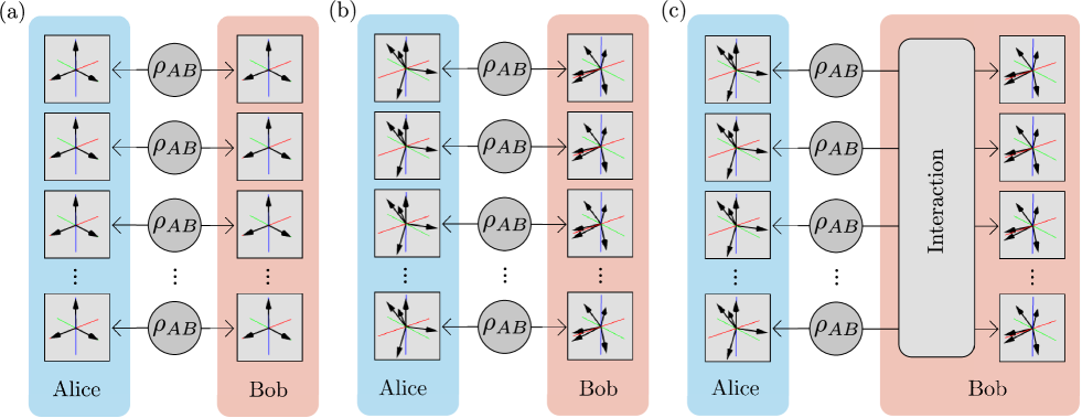
Figure 1: This diagram shows the different definitions of classical correlations (CC) of a bipartite state $\rho_{AB}$, that Alice and Bob share many copies of. (a) Alice and Bob perform projective measurements. The maximum classical mutual information (MI) of their measurement outcomes is the symmetric CC. (b) Alice and Bob perform POVM measurements. The maximum classical MI of their measurement outcomes is the extended symmetric CC. (c) Alice and Bob perform POVM measurements, but Bob is allowed to interact all his states beforehand. This is equivalent to the asymmetric CC.

II.2.1 Symmetric quantum discord

We first consider the approach of Ref. Maziero et al. (2010), which was also used by Ref. Rulli and Sarandy (2011) to define the multipartite global quantum discord.

Equation (3) can be written in an alternative form. Suppose Alice performs a projective measurement on her subsystem of $\rho_{AB}$. A projective measurement is a POVM in which the elements are $\Pi_{a}=\ket{a}\bra{a}$ where $\{\ket{a}\}$ are a set of states that form an orthonormal basis. The state after the measurement will be a classical-quantum state given by

$$\phi_{A}(\rho_{AB})=\sum_{a}p_{a}\ket{a}\bra{a}\otimes\rho_{B|a}.$$ (6)

Here we have defined $\phi_{A}(\rho)$ to be the state $\rho$ becomes after a measurement on $A$. After the measurement, $A$ will be diagonal in the measurement basis:

$$\phi_{A}(\rho_{A})=\sum_{a}p_{a}\ket{a}\bra{a},$$ (7)

with entropy $S(\phi_{A}(\rho_{A}))=\sum_{a}h(p_{a})$. $B$ will be unchanged by a measurement on $A$: $\phi_{A}(\rho_{B})=\rho_{B}$. Since $\phi_{A}(\rho_{AB})$ is a classical-quantum state, we can write its entropy as

$$S(\phi_{A}(\rho_{AB}))=S(\phi_{A}(\rho_{A}))+\sum_{a}p_{a}S(\rho_{B|a}).$$ (8)

The asymmetric CC Eq. (3), with the optimisation over projective measurements instead of POVMs, is equivalent to the quantum MI of state $\phi_{A}(\rho_{AB})$ maximized over all projective measurements on $A$.

$$\max_{\{\ket{a}\}}I_{Q}(\phi_{A}(\rho_{AB}))$$ (9)

$$=\max_{\{\ket{a}\}}S(\phi_{A}(\rho_{A}))+S(\phi_{A}(\rho_{B}))-S(\phi_{A}(\rho_{AB}))$$ (10)

$$=\max_{\{\ket{a}\}}S(\phi_{A}(\rho_{A}))+S(\rho_{B})-S(\phi_{A}(\rho_{A}))-\sum_{a}p_{a}S(\rho_{B|a})$$ (11)

$$=S(B)-\min_{\{\ket{a}\}}\sum_{a}p_{a}S(\rho_{B|a})$$ (12)

The interpretation of the measurement that maximizes the above is that it is the projective measurement that least disturbs the state, that is, the projective measurement that results in the least loss in quantum MI.

The extension to a symmetric version is simple. In this case, a projective measurement is performed on both $A$ and $B$. After the measurement, $\rho_{AB}$ will became be a classical-classical state given by

$$\phi_{AB}(\rho_{AB})=\sum_{a,b}p_{ab}\ket{a}\bra{a}\otimes\ket{b}\bra{b}.$$ (13)

where $p_{ab}=\Tr{\rho_{AB}\ket{a}\bra{a}\otimes\ket{b}\bra{b}}$. The symmetric CC is given by

$$J_{S}(A;B) =\max_{\{\ket{a}\},\{\ket{b}\}}I_{Q}(\phi_{AB}(\rho_{AB}))$$ (14)

$$=\max_{\{\ket{a}\},\{\ket{b}\}}S(\phi(\rho_{A}))+S(\phi(\rho_{B}))-S(\phi(\rho_{AB}))$$ (15)

$$=\max_{\{\ket{a}\},\{\ket{b}\}}\sum_{a}h(p_{a})+\sum_{b}h(p_{b})-\sum_{a,b}h(p_{ab})$$ (16)

The symmetric QD is

$$\delta_{S}(A;B)=I_{Q}(A;B)-J_{S}(A;B).$$ (17)

The interpretation of the symmetric QD is that it is the smallest loss in quantum MI after local projective measurements on $A$ and $B$.

The asymmetric CC and symmetric CC are related by the inequality

$$J_{S}(A;B)\leq J(A|B).$$ (18)

This inequality results from the fact that the quantum mutual information of a state cannot increase under a measurement of one subsystem. Hence, the correlations after measurement reduce (or remain the same) if Bob does a measurement in addition to Alice.

II.2.2 Extended symmetric quantum discord

An alternative way of defining the classical correlations is using the classical mutual information Piani et al. (2008); Wu et al. (2009); Terhal et al. (2002). This turns out to be equivalent to symmetric QD but is defined when the measurement is any POVM.

Let $\mathcal{A}$ be the random variable that describes measurement outcomes $a$ on state $A$, and $\mathcal{B}$ be the random variable that describes measurement outcomes $b$ on state $B$. The classical MI between $\mathcal{A}$ and $\mathcal{B}$ is

$$I_{C}(\mathcal{A},\mathcal{B})=H(\mathcal{A})+H(\mathcal{B})-H(\mathcal{AB}),$$ (19)

where $H(X)$ is the Shannon entropy of variable $X$. It is defined by

$$H(X)=\sum_{x}h(p_{x}),$$ (20)

where $p_{x}$ is the probability that $X=x$.

We introduce a new measure of the classical correlations $J_{ES}$, we call the extended symmetric CC. It is defined as the maximum classical mutual information between the measurement outcomes made on $A$ and $B$, maximized over all POVM measurements.

$$J_{ES}(A;B) =\max_{\{\Pi_{a}\},\{\Pi_{b}\}}I_{C}(\mathcal{A},\mathcal{B})$$ (21)

$$=\max_{\{\Pi_{a}\},\{\Pi_{b}\}}\sum_{a}h(p_{a})+\sum_{b}h(p_{b})-\sum_{a,b}h(p_{ab})$$ (22)

$$=\max_{\{\Pi_{a}\},\{\Pi_{b}\}}\sum_{b}h(p_{b})-\sum_{a}p_{a}\sum_{b}h(p_{b|a})$$ (23)

This quantity is symmetric, because classical mutual information is symmetric. We then define the extended symmetric QD as

$$\delta_{ES}(A;B)=I_{Q}(A;B)-J_{ES}(A;B).$$ (24)

The same quantity is being maximised in Eqs. (16) and (22). This implies two things. Firstly, there is an equivalent interpretation of the symmetric CC as the classical MI between measurement outcomes on $A$ and $B$, maximised over local projective measurements. Secondly, we have the inequality,

$$J_{ES}(A;B)\geq J_{S}(A;B),$$ (25)

because projective measurements are a subset of POVMs. The extended symmetric CC can be viewed as an extension of the symmetric CC, in that it extends the definition of symmetric CC to general POVMs.

II.3 Comparison of CC measures

Figure 1 shows the interpretations of the three different CC quantities. Suppose Alice and Bob share $n$ copies of a bipartite state $\rho_{AB}$. Alice measures each copy separately using the same measurement. Let $\mathcal{A}$ be the random variable that describes her measurement outcomes. Bob does the same thing, and $\mathcal{B}$ describes his measurement outcomes. The maximum classical MI between $\mathcal{A}$ and $\mathcal{B}$ is the symmetric CC if Alice and Bob can perform projective measurements, extended CC if they can do any POVM measurements.

Now suppose Bob is allowed to interact all his copies before he measures them, as in Figure 1(c). Can he gain any more information about Alice’s measurements outcomes? The answer is yes, provided Alice sends Bob some additional classical information. The maximum information Bob can obtain about Alice’s measurement outcome subtracting the additional classical information Alice sends is equal to the asymmetric CC. A protocol that achieves this rate is described in Ref. Devetak and Winter (2003).

These quantities are related by

$$\min\left(J(A|B),J(B|A)\right)\geq J_{ES}(A;B)\geq J_{S}(A;B)\;.$$ (26)

II.4 Multipartite quantum discord

The extended symmetric CC and QD can be defined for multipartite states Piani et al. (2008), using multipartite extensions of the classical MI and quantum MI Watanabe (1960). Let a multipartite state $\rho_{\vec{A}}$ be distributed to $n$ parties, where $\vec{A}=[A_{1},A_{2},\ldots,A_{n}]$. Let $A_{i}$ denote the subsystem received by $i$-th party. Each party measures their subsystem, and $\mathcal{A}_{i}$ denotes the random variable that describes measurement outcomes $a_{i}$ on subsystem $A_{i}$. The multipartite classical MI is

$$I_{C}(\mathcal{A}_{1};\mathcal{A}_{2};\ldots;\mathcal{A}_{n})=\sum_{i=1}^{n}H(\mathcal{A}_{i})-H(\mathcal{A}_{1}\mathcal{A}_{2}\ldots\mathcal{A}_{n}),$$ (27)

The $n$-partite extended symmetric CC of state $\rho_{\vec{A}}$ is

$$J_{ES}(A_{1};A_{2};\ldots;A_{n})$$

$$= \max_{\{\Pi_{a_{1}}\},\{\Pi_{a_{2}}\},\ldots,\{\Pi_{a_{n}}\}}I_{C}(\mathcal{A}_{1};\mathcal{A}_{2};\ldots;\mathcal{A}_{n}),$$ (28)

The maximization is over local POVM measurements $\{\Pi_{a_{i}}\}$ performed on subsystems $A_{i}$.

$$H(\mathcal{A}_{i})=\sum_{a_{i}}h(p_{a_{i}}),$$ (29)

where $p_{a_{i}}=\Tr{\rho_{A_{i}}\Pi_{a_{i}}}$.

$$H(\vec{\mathcal{A}})=\sum_{a_{1}}\sum_{a_{2}}\ldots\sum_{a_{n}}h(p(a_{1},a_{2},\ldots,a_{n})),$$ (30)

where $p(a_{1},a_{2},\ldots,a_{n})=\Tr{\rho_{\vec{A}}\Pi_{a_{1}}\Pi_{a_{2}}\ldots\Pi_{a_{n}}}$.

Similarly, the multipartite quantum MI is given by

$$I_{Q}(A_{1};A_{2};\ldots;A_{n})=\sum_{i=1}^{n}S(A_{i})-S(A_{1}A_{2}\ldots A_{n}).$$ (31)

This allows us to define the multipartite extended symmetric QD by

$$\delta_{ES}(A_{1};A_{2};\ldots;A_{n})=I_{Q}(A_{1};A_{2};\ldots;A_{n})\\ -J_{ES}(A_{1};A_{2};\ldots;A_{n}).$$ (32)

Rulli and Sarandy defined a similar quantity called the global quantum discord Rulli and Sarandy (2011), but the measurements are restricted to projective measurements. The multipartite extended symmetric QD can be viewed as an extension of the global quantum discord to general POVM measurements.

III Gaussian multipartite CC and QD

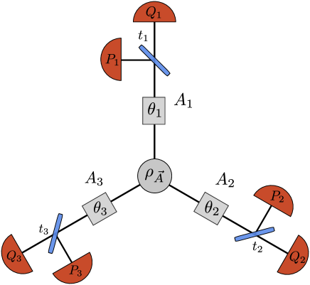
Figure 2: The three modes of a tripartite Gaussian state $\rho_{\vec{A}}$ are distributed to three parties. Each party does a Gaussian measurement on their subsystem $A_{i}$. A Gaussian measurement of a single-mode Gaussian state consists of a phase shift of $\theta_{i}$ followed by a beam splitter with transmissivity $0\leq t_{i}\leq 1$ followed by measurement of the $Q$ and $P$ quadratures. The maximum classical mutual information between the measurement outcomes gives the multipartite Gaussian CC (Eq. (III)).

Let us define the Gaussian multipartite CC $J_{G}(\vec{A})$ to be the maximum classical MI achievable when the measurement on each subsystem are restricted to Gaussian measurements. Hence $J_{G}(\vec{A})$ is equivalent to Eq. (II.4) except the maximization is over Gaussian POVMs, rather than all POVMs.

We introduce the Gaussian multipartite QD given by

$$\delta_{G}(\vec{A})=I_{Q}(\vec{A})-J_{G}(\vec{A}).$$ (33)

Suppose $n$ parties each receive one mode of an $n$-partite Gaussian state. We now describe how to calculate the Gaussian multipartite QD in this situation. Each party performs a Gaussian measurement on their subsystem. A Gaussian measurement of a single-mode Gaussian state can be described by a phase shift $\theta_{i}$ followed by a beam splitter with transmissivity $0\leq t_{i}\leq 1$ and orthogonal quadrature measurements $Q_{i}$ and $P_{i}$ on the outputs of the beam splitter. Figure 2 shows a diagram of the measurements performed for the case of a tripartite Gaussian state.

The Gaussian multipartite CC of a bipartite state is

$$J_{G}(A_{1},A_{2})=\max_{\theta_{1},t_{1},\theta_{2},t_{2}}I_{C}(Q_{2};Q_{1}P_{1})+I_{C}(P_{2}|Q_{2};Q_{1}P_{1})\\ =\max_{\theta_{1},t_{1},\theta_{2},t_{2}}\big{[}G(Q_{2})-G(Q_{2}|Q_{1}P_{1})+G(P_{2}|Q_{2})\\ -G(P_{2}|Q_{1}P_{1}Q_{2})\big{]}\;,$$ (34)

where $G(Q)$ is the differential entropy of $Q$. The measurement outcome of a Gaussian measurement performed on a Gaussian state are normally distributed. Consider a random variable $X$ that is normally distributed. The probability density of $X$ is

$$p_{x}=\frac{1}{\sqrt{2\pi V_{X}}}\exp(-\frac{(x-\mu_{X})^{2}}{2V_{X}}),$$ (35)

where $\mu_{X}$ is the mean of $X$ and $V_{X}$ is the variance of $X$. The differential entropy of $X$ is

$$G(V_{X}) =-\int_{-\infty}^{\infty}p_{x}\log_{2}p_{x}\;dx$$ (36)

$$=\frac{1}{2}\log_{2}(2\pi eV_{X}),$$ (37)

Note that the differential entropy of $X$ does not depend on the mean of $X$.

There is an additional property that allows us to simplify Eq. (34). The conditional variances do not depend on other measurement outcomes. For example, the variance of $Q_{2}$ conditioned on the measurement outcomes of $Q_{1}$ and $P_{1}$, denoted $V_{Q_{2}|Q_{1}P_{1}}$, will be a constant independent of the measurement outcomes of $Q_{1}$ and $P_{1}$. Therefore, Eq. (34) becomes

$$J_{G}(A_{1},A_{2})=\max_{\theta_{1},t_{1},\theta_{2},t_{2}}\Big{[}G(V_{Q_{2}})\\ +G(V_{P_{2}|Q_{2}})-G(V_{Q_{2}|Q_{1}P_{1}})-G(V_{P_{2}|Q_{1}P_{1}Q_{2}})\Big{]}.$$ (38)

The extension to $n$-partite states is

$$J_{G}(\vec{A})= \ \max_{\theta_{1},t_{1},\theta_{2},t_{2},\ldots,\theta_{n},t_{n}}\big{[}$$

$$\ H(\mathcal{A}_{2})-H(\mathcal{A}_{2}|\mathcal{A}_{1})$$

$$+ \ H(\mathcal{A}_{3})-H(\mathcal{A}_{3}|\mathcal{A}_{2}\mathcal{A}_{1})$$

$$\vdots$$

$$+ \ H(\mathcal{A}_{n})-H(\mathcal{A}_{n}|\mathcal{A}_{n-1}\mathcal{A}_{n-2}\ldots A_{1})\big{]},$$ (39)

where

$$H(\mathcal{A}_{i})=G(V_{Q_{i}})+G(V_{P_{i}|Q_{i}})$$ (40)

and

$$H(\mathcal{A}_{i}|\mathcal{A}_{i-1}\ldots\mathcal{A}_{1})=G(V_{Q_{i}|Q_{i-1}P_{i-1}\ldots Q_{1}P_{1}})\\ +G(V_{P_{i}|Q_{i}Q_{i-1}P_{i-1}\ldots Q_{1}P_{1}}).$$ (41)

The calculation of Eq. (III) involves an optimization over $2n$ variables. We will demonstrate the calculation of Eq. (III) for some states.

III.1 Properties

We state and prove several desirable properties of the the Gaussian multipartite CC and QD.

1. Gaussian multipartite CC is symmetric. This is true because the classical mutual information is symmetric.

2. The Gaussian multipartite QD is zero for product states. This follows from the nonnegativity of the Gaussian multipartitie QD and the fact that quantum mutual information is zero for product states.

3. The Gaussian multipartite CC does not increase under local Gaussian operations. This is because local Gaussian operations can be considered part of the measurements.

III.2 Example: two-mode EPR state

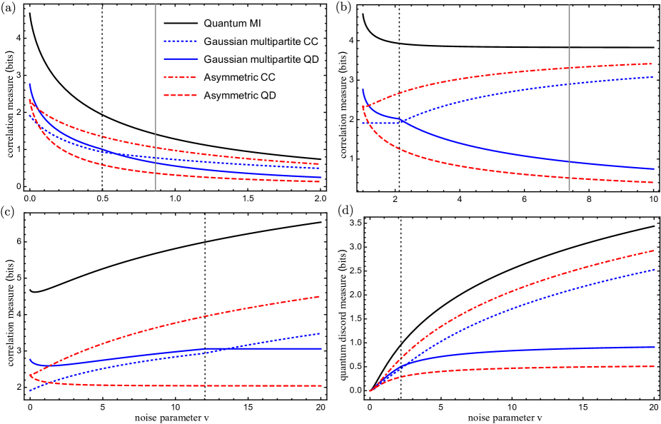
Figure 3: This plot shows the correlations present in a two-mode squeezed EPR state (Eq. (42)) with $r=1$ subjected to (a) uncorrelated noise, (b) multiplicative noise, and (c) correlated noise. Also shown is (d) the correlations present in a vacuum state subjected to correlated noise. If $v$ is less than the dashed vertical line, the measurements that attains the Gaussian multipartite QD and CC are homodyne measurements, otherwise the measurements are heterodyne measurements. For $v$ less than the solid vertical line the state is entangled, otherwise separable. For (c), the state is entangled for all $v$. For (d), the state is separable for all $v$.

Consider a two-mode Einstein-Podolsky-Rosen (EPR) state. The covariance of the quadratures of the EPR state is Weedbrook et al. (2012)

$$V_{EPR}=\begin{pmatrix}\cosh 2r&0&\sinh 2r&0\\ 0&\cosh 2r&0&-\sinh 2r\\ \sinh 2r&0&\cosh 2r&0\\ 0&-\sinh 2r&0&\cosh 2r\end{pmatrix}.$$ (42)

The measurement that attains the Gaussian multipartite CC will have phase shifts of zero, i.e. $\theta_{1}=\theta_{2}=0$. In fact, the phase shifts will be zero for any quadrature covariance matrix that has zero covariance between $Q$ and $P$ quadratures. Values of the other parameters $t_{1}$ and $t_{2}$ were found by performing the optimisation analytically. The optimum occurs when $t_{1}=t_{2}=0$ or $1$, giving $J_{G}(A_{1},A_{2})=\log_{2}(\cosh 2r)$. This corresponds to performing homodyne measurements on each subsystem.

If $r=1$ then $J_{G}=1.912$. If instead we consider the extended symmetric CC, where the measurements are not restricted to Gaussian measurements we obtain $J_{ES}=2.337$. This is obtained when both parties measure in the Fock number state basis. By restricting to Gaussian measurements we reduce the amount of classical correlations that can be seen. The calculation of Gaussian classical correlations however, is much simpler. In general, it is nontrivial to find the measurement that optimises $J_{ES}$. Additionally, Gaussian measurements have the added bonus of being easy to do experimentally, requiring only linear optical elements and homodyne measurements.

III.3 Example: noisy EPR state

We calculated the multipartite Gaussian CC and QD for an EPR state subjected to three different types of noise, which is plotted in Fig. 3(a,b,c). A useful result, derived by Ref. Mišta Jr. and Tatham (2016) for the calculation of Gaussian intrinsic entanglement, is that for a state with quadrature covariance matrix

$$\begin{pmatrix}a&0&c_{x}&0\\ 0&a&0&c_{p}\\ c_{x}&0&b&0\\ 0&c_{p}&0&b\end{pmatrix}$$ (43)

with $c_{x}\geq|c_{p}|\geq 0$, the Gaussian multipartite CC of this state is obtained by a homodyne measurements of the $Q$ quadratures (corresponding to the measurement when $t_{1}=t_{2}=1$) if

$$\sqrt{\frac{a}{b}}+\sqrt{\frac{b}{a}}+\frac{1}{\sqrt{{a}{b}}}-\sqrt{ab-c_{x}^{2}}\geq 0.$$ (44)

Since the two-mode states we consider are symmetric in the $Q$ and $P$ quadratures, homodyne measurements of the $P$ quadratures (corresponding to the measurement when $t_{1}=t_{2}=0$) gives the same classical MI. When the above inequality is not satisfied, numerical optimisation revealed that for all two mode states we considered the optimal measurement is a heterodyne measurement of both modes (corresponding to $t_{1}=t_{2}=1/2$).

As is typical of quantum discord quantities, we observe that when noise is increased sufficiently such that the state becomes separable, determined using Duan’s inseparability criterion Duan et al. (2000), there is still a nonzero amount of Gaussian multipartite QD.

We also calculate the asymmetric CC and QD. For the states we consider, the asymmetric QD is equal to the asymmetric Gaussian QD, and additionally this is obtained by a heterodyne measurement on one of the subsystems Pirandola et al. (2014). We are unaware of any simple means of calculating the symmetric QD or extended symmetric QD for Gaussian states, so we chose not to calculate these quantities.

III.3.1 Uncorrelated noise

Firstly let us consider the case in which uncorrelated quadrature noise is added to each mode of the EPR state. The quadrature covariance matrix of the resulting state is $V_{EPR}+vI_{4}$ where $I_{4}$ is the 4-by-4 identity matrix, and $v\geq 0$ is a parameter that controls the amount of noise. A plot of correlation is shown in Fig. 3(a). The total correlations, as measured by the quantum MI, decreases as $v$ increases. The Gaussian multipartite CC, Gaussian multipartite QD, assymetric CC, and symmetric CC also all decrease as the noise increases.

III.3.2 Multiplicative noise

Now consider the case in which the quadrature covariance is multiplied by a factor $v\geq 1$, so the quadrature covariance matrix is $vV_{EPR}$. This type of noise is realised if the EPR state is generated by mixing on a beam splitter two squeezed states that are impure. Then $v$ is equal to multiplication of the squeezed state quadrature variances. The information quantities are shown in Fig. 3(b). The total correlations, as measured by the quantum MI, decreases as $v$ increases. Despite this, the Gaussian multipartite CC and asymmetric CC do increase, however this is at the expense of the Gaussian multipartite QD and asymmetric QD, which decrease.

For $v$ less than some value, the Gaussian multipartite CC is constant. This is the region in which a homodyne measurement is optimal.

III.3.3 Correlated noise

The third case we consider is adding classically correlated noise to $Q$ quadratures of each mode, and classically anticorrelated noise to the $P$ quadratures. The quadrature covariances of the resulting state is

$$V_{EPR}+\begin{pmatrix}v&0&v&0\\ 0&v&0&-v\\ v&0&v&0\\ 0&-v&0&v\end{pmatrix}.$$ (45)

The information quantities are shown in Fig. 3(c). Unsurprisingly, the Gaussian multipartite CC and the asymmetric CC increase as a function of $v$, because we are adding classically correlated noise.

Adding correlated noise initially reduces the asymmetric QD and Gaussian multipartite QD, which also results in a dip in the quantum MI at the start. The heterodyne measurement is much better for detecting the added classical correlations, so when the heterodyne measurement is optimal the Gaussian multipartite QD is almost constant. For large $v$, the asymmetric QD and Gaussian multipartite QD appear almost constant but they are in fact slowly increasing.

It is perhaps counterintuitive that classically correlated noise can increase quantum discord. This can be more easily seen in Fig. 3(d), where classically correlated noise is added to a vacuum state. The state initially has zero correlations, but when the noise is added, all the correlation measures increase, including Gaussian multipartite QD and asymmetric QD. Generating a state with nonzero assymetric QD in this manner was done experimentally by Gu et al. (2012).

III.4 Example: noisy Gaussian tripartite GHZ state

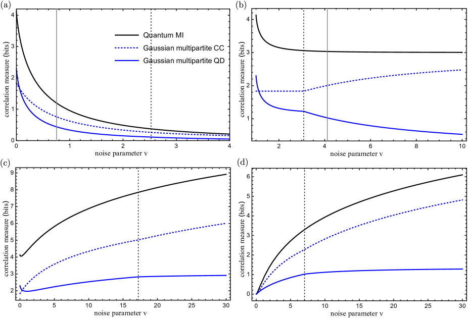
Figure 4: The correlations present in a three-mode Gaussian GHZ state (Eq. (46)) with $a=2$ subjected to (a) uncorrelated noise, (b) multiplicative noise, (c) correlated noise, and (d) the correlations present in a three-mode vacuum state subjected to correlated noise. If $v$ is less than the dashed vertical line, the measurements that attains the Gaussian multipartite CC and QD are homodyne measurements. For $v$ less than the solid vertical line the state is entangled, otherwise separable. For (c), the state is entangled for all $v$. For (d), the state is separable for all $v$.

The tripartite Gaussian state equivalent to the three-qubit GHZ and W states is a state with quadrature covariance matrix given by Adesso et al. (2006)

$$V_{GHZ}=\begin{pmatrix}a&0&c^{+}&0&c^{+}&0\\ 0&a&0&c^{-}&0&c^{-}\\ c^{+}&0&a&0&c^{+}&0\\ 0&c^{-}&0&a&0&c^{-}\\ c^{+}&0&c^{+}&0&a&0\\ 0&c^{-}&0&c^{-}&0&a\\ \end{pmatrix}$$ (46)

where

$$c^{\pm}=\frac{a^{2}-1\pm\sqrt{(a^{2}-1)(9a^{2}-1)}}{4a}.$$ (47)

Like for the two-mode case, we calculate the Gaussian multipartite CC and QD for the state subjected to three different types of noise. Figure 4 shows our results. To determine whether a state is separable, we use the method of  Giedke et al. (2001).

III.4.1 Uncorrelated noise

Consider a three-mode GHZ state with uncorrelated quadrature noise added to each of the three modes. The resulting state has a quadrature covariances $V_{GHZ}+vI_{6}$ where $I_{6}$ is the 6-by-6 identity matrix. Figure 4(a) is a plot of the information quantities. Just as in the two mode case, the quantum MI, Gaussian multipartite CC and QD all decrease as $v$ increases.

III.4.2 Multiplicative noise

The information quantities for a three-mode GHZ state with multiplicative noise, i.e. a state with covariance matrix $vV_{GHZ}$, are shown in Fig. 4(b). Similar to the two made case, this type of noise reduces the total correlations (quantum MI) and Gaussian multipartite QD, while at the same time increasing the Gaussian multipartite CC when $v$ is large. Just as in the two-mode case, homodyne measurements on each mode give the a classical mutual information that does not depend on $v$. Hence, the Gaussian multipartite CC is constant when the optimal measurement consists of homodyne measurements, which for $a=2$, is when $v<3.082$.

III.4.3 Correlated noise

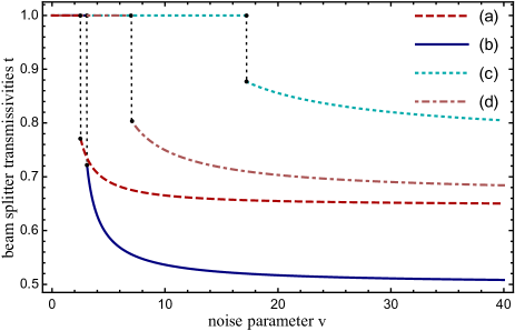
Figure 5: This plot shows the beam splitter transmissivities $t_{1}=t_{2}=t_{3}=t$ for the measurement that attains the Gaussian multipartite CC and QD for the corresponding plots in Fig. 4.

Now we consider the case in which correlated noise is added to the $Q$ quadratures of each mode and anticorrelated noise is added to the $P$ quadratures. The resulting state has quadrature covariances

$$V_{GHZ}+v\begin{pmatrix}1&0&1&0&1&0\\ 0&1&0&-0.5&0&-0.5\\ 1&0&1&0&1&0\\ 0&-0.5&0&1&0&-0.5\\ 1&0&1&0&1&0\\ 0&-0.5&0&-0.5&0&1\end{pmatrix}.$$ (48)

Note that the matrix contains $-0.5$ terms. This is the largest anticorrelation that three classical variables with variance of 1 can have.

The information quantities for this state are shown in Fig. 4(c). We notice three properties that are the same as the two-mode case. (1) Initially there is a dip in the quantum MI and Gaussian multipartite QD. (2) The Gaussian mulitpartite CC increase as a function of $v$. (3) While homodyne measurements are optimal, after the initial dip, the multipartite QD increases as a function of $v$. When homodyne measurements are not optimal, the mulitpartite QD appears almost constant but is in fact slowly increasing.

Figure 4(d) shows the correlations present when the correlated noise is added to a three-mode vacuum state. Just as in the two-mode case, the Gaussian multipartite QD discord is nonzero for $v\geq 0$, despite the fact that the state is separable.

III.4.4 Measurements

In all of the cases described above, for small $v$, the measurement that attains the Gaussian multipartite CC and QD consists of homodyne measurements of the $Q$ quadrature on each mode ($t_{1}=t_{2}=t_{3}=1$). Homodyne measurements of the $P$ quadratures does not give the same classical MI because there is an asymmetry in the $Q$ and $P$ quadratures of the Gaussian GHZ state; the anticorrelations of the $P$ quadratures are less than the correlations of the $Q$ quadratures.

For large $v$, the optimal measurement consists of beam splitter transmisivities $t_{1}=t_{2}=t_{3}=t$ where $t<1$. In stark contrast to the two-mode case, this value of $t$ depends on $v$. A plot the relationship between $v$ and $t$ is shown in Fig. 5. There is a discontinuity at the point where homodyne measurements are no longer optimal; the value of $t$ abruptly changes from 1 to some value that is less than 1. Note that there is also a discontinuity in the two made case, in which $t$ changes from 1 or 0 to $1/2$.

IV Conclusion

We have introduced a new measure of the classical correlations of a multipartite Gaussian state, defined as the maximum classical MI between Gaussian measurement outcomes performed on each subsystem. We introduce a new measure of multipartite Gaussian QD defined by subtracting the multipartite Gaussian CC from the multiparite quantum MI of the state. The Gaussian multipartite CC is easy to calculate, requiring an optimisation over at most $2n$ variables for an $n$-mode Gaussian state. We envisage this measure being relevant in Gaussian quantum information experiments that do not use any non-Gaussian measurements.

We calculated the Gaussian multipartite CC and QD for a two-mode EPR state and a three-mode Gaussian GHZ state subjected to different types of noise.

References

- Horodecki et al. (2009) R. Horodecki, P. Horodecki, M. Horodecki, and K. Horodecki, “Quantum entanglement,” Rev. Mod. Phys. 81, 865 (2009).
- Bennett et al. (1999) Charles H Bennett, David P DiVincenzo, Christopher A Fuchs, Tal Mor, Eric Rains, Peter W Shor, John A Smolin, and William K Wootters, “Quantum nonlocality without entanglement,” Physical Review A 59, 1070 (1999).
- Ollivier and Zurek (2001) H. Ollivier and W. H. Zurek, “Quantum discord: a measure of the quantumness of correlations,” Phys. Rev. Lett. 88, 017901 (2001).
- Henderson and Vedral (2001) L. Henderson and V. Vedral, “Classical, quantum and total correlations,” J. Phys. A: Math. Gen. 34, 6899 (2001).
- Maziero et al. (2010) J. Maziero, L. C. Celeri, and R. M. Serra, “Symmetry aspects of quantum discord,” arXiv preprint arXiv:1004.2082 (2010).
- Piani et al. (2008) M. Piani, P. Horodecki, and R. Horodecki, “No-local-broadcasting theorem for multipartite quantum correlations,” Phys. Rev. Lett. 100, 090502 (2008).
- Wu et al. (2009) S. Wu, U. V. Poulsen, and K. Mølmer, “Correlations in local measurements on a quantum state, and complementarity as an explanation of nonclassicality,” Phys. Rev. A 80, 032319 (2009).
- Terhal et al. (2002) B. M. Terhal, M. Horodecki, D. W. Leung, and D. P. DiVincenzo, “The entanglement of purification,” J. Math. Phys. 43, 4286–4298 (2002).
- Rulli and Sarandy (2011) C. C. Rulli and M. S. Sarandy, “Global quantum discord in multipartite systems,” Phys. Rev. A 84, 042109 (2011).
- Huang (2014) Yichen Huang, “Computing quantum discord is NP-complete,” New J. Phys. 16, 033027 (2014).
- Giorda and Paris (2010) P. Giorda and M. G. A. Paris, “Gaussian quantum discord,” Phys. Rev. Lett. 105, 020503 (2010).
- Adesso and Datta (2010) G. Adesso and A. Datta, “Quantum versus classical correlations in gaussian states,” Phys. Rev. Lett. 105, 030501 (2010).
- Modi et al. (2010) K. Modi, T. Paterek, W. Son, V. Vedral, and M. Williamson, “Unified view of quantum and classical correlations,” Phys. Rev. Lett. 104, 080501 (2010).
- Dakić et al. (2010) B. Dakić, V. Vedral, and Č. Brukner, “Necessary and sufficient condition for nonzero quantum discord,” Phys. Rev. Lett. 105, 190502 (2010).
- Oppenheim et al. (2002) J. Oppenheim, M. Horodecki, P. Horodecki, and R. Horodecki, “Thermodynamical approach to quantifying quantum correlations,” Phys. Rev. Lett. 89, 180402 (2002).
- Luo and Fu (2011) S. Luo and S. Fu, “Measurement-induced nonlocality,” Phys. Rev. Lett. 106, 120401 (2011).
- Girolami et al. (2014) D. Girolami, A. M. Souza, V. Giovannetti, T. Tufarelli, J. G. Filgueiras, R. S. Sarthour, D. O. Soares-Pinto, I. S. Oliveira, and G. Adesso, “Quantum discord determines the interferometric power of quantum states,” Phys. Rev. Lett. 112, 210401 (2014).
- Bera et al. (2018) A. Bera, T. Das, D. Sadhukhan, S. S. Roy, A. Sen(De), and U. Sen, “Quantum discord and its allies: a review of recent progress,” Reports on Progress in Physics 81, 024001 (2018).
- Devetak and Winter (2003) I. Devetak and A. Winter, “Classical data compression with quantum side information,” Phys. Rev. A 68, 042301 (2003).
- Watanabe (1960) S. Watanabe, “Information theoretical analysis of multivariate correlation,” IBM Journal of research and development 4, 66–82 (1960).
- Weedbrook et al. (2012) C. Weedbrook, S. Pirandola, R. García-Patrón, N. J. Cerf, T. C. Ralph, J. H. Shapiro, and S. Lloyd, “Gaussian quantum information,” Rev. Mod. Phys. 84, 621–669 (2012).
- Mišta Jr. and Tatham (2016) L. Mišta Jr. and R. Tatham, “Gaussian intrinsic entanglement,” Phys. Rev. Lett. 117, 240505 (2016).
- Duan et al. (2000) L.-M. Duan, G. Giedke, J. I. Cirac, and P. Zoller, “Inseparability criterion for continuous variable systems,” Phys. Rev. Lett. 84, 2722 (2000).
- Pirandola et al. (2014) S. Pirandola, G. Spedalieri, S. L. Braunstein, N. J. Cerf, and S. Lloyd, “Optimality of gaussian discord,” Phys. Rev. Lett. 113, 140405 (2014).
- Gu et al. (2012) Mile Gu, Helen M Chrzanowski, Syed M Assad, Thomas Symul, Kavan Modi, Timothy C Ralph, Vlatko Vedral, and Ping Koy Lam, “Observing the operational significance of discord consumption,” Nature Physics 8, 671 (2012).
- Adesso et al. (2006) G. Adesso, A. Serafini, and F. Illuminati, “Multipartite entanglement in three-mode gaussian states of continuous-variable systems: Quantification, sharing structure, and decoherence,” Phys. Rev. A 73, 032345 (2006).
- Giedke et al. (2001) G. Giedke, B. Kraus, M. Lewenstein, and J. I. Cirac, “Separability properties of three-mode gaussian states,” Phys. Rev. A 64, 052303 (2001).