Variance Reduction in Stochastic Particle-Optimization Sampling

Abstract

Stochastic particle-optimization sampling (SPOS) is a recently-developed scalable Bayesian sampling framework that unifies stochastic gradient MCMC (SG-MCMC) and Stein variational gradient descent (SVGD) algorithms based on Wasserstein gradient flows. With a rigorous non-asymptotic convergence theory developed recently, SPOS avoids the particle-collapsing pitfall of SVGD. Nevertheless, variance reduction in SPOS has never been studied. In this paper, we bridge the gap by presenting several variance-reduction techniques for SPOS. Specifically, we propose three variants of variance-reduced SPOS, called SAGA particle-optimization sampling (SAGA-POS), SVRG particle-optimization sampling (SVRG-POS) and a variant of SVRG-POS which avoids full gradient computations, denoted as SVRG-POS⁺. Importantly, we provide non-asymptotic convergence guarantees for these algorithms in terms of 2-Wasserstein metric and analyze their complexities. Remarkably, the results show our algorithms yield better convergence rates than existing variance-reduced variants of stochastic Langevin dynamics, even though more space is required to store the particles in training. Our theory well aligns with experimental results on both synthetic and real datasets.

Keywords

Stochastic particle-optimization sampling; Variance Reduction; Non-asymptotic convergence guarantees; 2-Wasserstein metric; Complexities;

1 Introduction

Sampling has been an effective tool for approximate Bayesian inference, which becomes increasingly important in modern machine learning. In the setting of big data, recent research has developed scalable Bayesian sampling algorithms such as stochastic gradient Markov Chain Monte Carlo (SG-MCMC) [21] and Stein variational gradient descent (SVGD) [15]. These methods have facilitated important real-world applications and achieved impressive results, such as topic modeling [10, 16], matrix factorization [2, 6, 1], differential privacy [20, 14], Bayesian optimization [19] and deep neural networks [13]. Generally speaking, these methods use gradient information of a target distribution to generate samples, leading to more effective algorithms compared to traditional sampling methods. Recently, [4] proposed a particle-optimization Bayesian sampling framework based on Wasserstein gradient flows, which unified SG-MCMC and SVGD in a new sampling framework called particle-optimization sampling (POS). Very recently, [23] discovered that SVGD endows some unintended pitfall, i.e. particles tend to collapse under some conditions. As a result, a remedy was proposed to inject random noise into SVGD update equations in the POS framework, leading to stochastic particle-optimization sampling (SPOS) algorithms [23]. Remarkably, for the first time, non-asymptotic convergence theory was developed for SPOS (SVGD-type algorithms) in [23].

In another aspect, in order to deal with large-scale datasets, many gradient-based methods for optimization and sampling use stochastic gradients calculated on a mini-batch of a dataset for computational feasibility. Unfortunately, extra variance is introduced into the algorithms, which would potentially degrade their performance. Consequently, variance control has been an important and interesting work for research. Some efficient solutions such as SAGA [5] and SVRG [11] were proposed to reduce variance in stochastic optimization. Subsequently, [9] introduced these techniques in SG-MCMC for Bayesian sampling, which also has achieved great success in practice.

Since SPOS has enjoyed the best of both worlds by combining SG-MCMC and SVGD, it will be of greater value to further reduce its gradient variance. While both algorithm and theory have been developed for SPOS, no work has been done to investigate its variance-reduction techniques. Compared with the research on SG-MCMC where variance reduction has been well explored by recent work such as [9, 3, 22], it is much more challenging for SPOS to control the variance of stochastic gradients. This is because from a theoretical perspective, SPOS corresponds to nonlinear stochastic differential equations (SDE), where fewer existing mathematical tools can be applied for theoretical analysis. Furthermore, the fact that many particles are used in an algorithm makes it difficult to improve its performance by adding modifications to the way they interact with each other.

In this paper, we take the first attempt to study variance-reduction techniques in SPOS and develop corresponding convergence theory. We adopt recent ideas on variance reduction in SG-MCMC and stochastic-optimization algorithms, and propose three variance-reduced SPOS algorithms, denoted as SAGA particle-optimization sampling (SAGA-POS), SVRG particle-optimization sampling (SVRG-POS) and a variant of SVRG-POS without full-gradient computations, denoted as SVRG-POS⁺. For all these variants, we prove rigorous theoretical results on their non-asymptotic convergence rates in terms of 2-Wasserstein metrics. Importantly, our theoretical results demonstrate significant improvements of convergence rates over standard SPOS. Remarkably, when comparing our convergence rates with those of variance-reduced stochastic gradient Langevin dynamics (SGLD), our theory indicates faster convergence rates of variance-reduced SPOS when the number of particles is large enough. Our theoretical results are verified by a number of experiments on both synthetic and real datasets.

2 Preliminaries

2.1 Stochastic gradient MCMC

In Bayesian sampling, one aims at sampling from a posterior distribution $p({\bm{\mathchar 28946\relax}}|\operatorname{\mathbf{X}})\propto p(\operatorname{\mathbf{X}}|{\bm{\mathchar 28946\relax}})p({\bm{\mathchar 28946\relax}})$, where ${\bm{\mathchar 28946\relax}}\in\mathbb{R}^{d}$ represents the model parameter, and $\operatorname{\mathbf{X}}\triangleq\{\operatorname{\mathbf{x}}_{j}\}_{j=1}^{N}$ is the dataset. Let $p({\bm{\mathchar 28946\relax}}|\operatorname{\mathbf{X}})=(1/Z)\exp(-U({\bm{\mathchar 28946\relax}}))$, where

$$U({\bm{\mathchar 28946\relax}})=-\log p(\operatorname{\mathbf{X}}|{\bm{\mathchar 28946\relax}})-\log p({\bm{\mathchar 28946\relax}})\triangleq-\sum_{j=1}^{N}\log p(\operatorname{\mathbf{x}}_{i}|{\bm{\mathchar 28946\relax}})-\log p({\bm{\mathchar 28946\relax}})$$

is referred to as the potential energy function, and $Z$ is the normalizing constant. We further define the full gradient $F$ and individual gradient $F_{j}$ used in our paper:

$$F_{j}({\bm{\mathchar 28946\relax}})\triangleq -\nabla_{{\bm{\mathchar 28946\relax}}}\log p(\operatorname{\mathbf{x}}_{j}|{\bm{\mathchar 28946\relax}})-\frac{1}{N}\nabla_{{\bm{\mathchar 28946\relax}}}\log p({\bm{\mathchar 28946\relax}})=\frac{1}{N}\nabla_{{\bm{\mathchar 28946\relax}}}U({\bm{\mathchar 28946\relax}})$$

$$F({\bm{\mathchar 28946\relax}})\triangleq \nabla_{{\bm{\mathchar 28946\relax}}}U({\bm{\mathchar 28946\relax}})=\sum_{j=1}^{N}F_{j}({\bm{\mathchar 28946\relax}})$$

We can define a stochastic differential equation, an instance of Itó diffusion whose stationary distribution equals to the target posterior distribution $p({\bm{\mathchar 28946\relax}}|\operatorname{\mathbf{X}})$. For example, consider the following 1st-order Langevin dynamic:

$$\mathrm{d}{\bm{\mathchar 28946\relax}}_{t}=-\beta^{-1}F({\bm{\mathchar 28946\relax}}_{t})\mathrm{d}t+\sqrt{2\beta^{-1}}\mathrm{d}\mathcal{W}_{t}~{},$$ (1)

where $t$ is the time index; $\mathcal{W}_{t}\in\mathbb{R}^{d}$ is $d$-dimensional Brownian motion, and $\beta$ a scaling factor. By the Fokker-Planck equation [12, 17], the stationary distribution of (1) equals to $p({\bm{\mathchar 28946\relax}}|\operatorname{\mathbf{X}})$.

SG-MCMC algorithms are discretized numerical approximations of Itó diffusions (1). To make algorithms efficient in a big-data setting, the computationally-expensive term $F$ is replaced with its unbiased stochastic approximations with a random subset of the dataset in each interation, e.g. $F$ can be approximated by a stochastic gradient:

$$\vspace{-0.3cm}G_{k}\triangleq\frac{N}{B}\sum_{j\in I_{k}}F_{j}(\mathchar 28946\relax_{k})=-\nabla\log p(\mathchar 28946\relax_{k})-\frac{N}{B}\sum_{j\in I_{k}}\nabla_{\mathchar 28946\relax_{k}}\log p(\operatorname{\mathbf{x}}_{j}|\mathchar 28946\relax_{k})$$

where $I_{k}$ is a random subset of $\{1,2,\cdots,N\}$ with size $B$. The above definition of $G_{k}$ reflects the fact that we only have information from $B\ll N$ data points in each iteration. This is the resource where the variance we try to reduce comes from. We should notice that $G_{k}$ is also used in standard SVGD and SPOS. As an example, SGLD is a numerical solution of (1), with an update equation: $\mathchar 28946\relax_{k+1}=\mathchar 28946\relax_{k}-\beta^{-1}G_{k}h+\sqrt{2\beta^{-1}h}{\bm{\xi}}_{k}$, where $h$ means the step size and ${\bm{\xi}}_{k}\sim\mathcal{N}(\mathbf{0},\operatorname{\mathbf{I}})$.

2.2 Stein variational gradient descent

Different from SG-MCMC, SVGD initializes a set of particles, which are iteratively updated to approximate a posterior distribution. Specifically, we consider a set of particles $\{{\bm{\mathchar 28946\relax}}^{(i)}\}_{i=1}^{M}$ drawn from some distribution $q$. SVGD tries to update these particles by doing gradient descent on the interactive particle system via

$${\bm{\mathchar 28946\relax}}^{(i)}\leftarrow{\bm{\mathchar 28946\relax}}^{(i)}+h\phi({\bm{\mathchar 28946\relax}}^{(i)}),~{}~{}\phi=\arg\max_{\phi\in\mathcal{F}}\{\dfrac{\partial}{\partial h}\textsf{KL}(q_{[h\phi]}||p)\}$$

where $\phi$ is a function perturbation direction chosen to minimize the KL divergence between the updated density $q_{[h\phi]}$ induced by the particles and the posterior $p({\bm{\mathchar 28946\relax}}|\operatorname{\mathbf{X}})$. The standard SVGD algorithm considers $\mathcal{F}$ as the unit ball of a vector-valued reproducing kernel Hilbert space (RKHS) $\mathcal{H}$ associated with a kernel $\kappa({\bm{\mathchar 28946\relax}},{\bm{\mathchar 28946\relax}}^{\prime})$. In such a setting, [15] shows that

$$\phi({\bm{\mathchar 28946\relax}})=\mathbb{E}_{{\bm{\mathchar 28946\relax}}^{\prime}\sim q}[\kappa({\bm{\mathchar 28946\relax}},{\bm{\mathchar 28946\relax}}^{\prime})F({\bm{\mathchar 28946\relax}}^{\prime})+\nabla_{{\bm{\mathchar 28946\relax}}^{\prime}}\kappa({\bm{\mathchar 28946\relax}},{\bm{\mathchar 28946\relax}}^{\prime})].$$ (2)

When approximating the expectation $\mathbb{E}_{{\bm{\mathchar 28946\relax}}^{\prime}\sim q}[\cdot]$ with an empirical distribution formed by a set of particles $\{{\bm{\mathchar 28946\relax}}^{(i)}\}_{i=1}^{M}$ and adopting stochastic gradients $G_{k}^{(i)}\triangleq\frac{N}{B}\sum_{j\in I_{k}}F_{j}(\mathchar 28946\relax_{k}^{(i)})$, we arrive at the following update for the particles:

$$\mathchar 28946\relax_{k+1}^{(i)}=\mathchar 28946\relax_{k}^{(i)}+\dfrac{h}{M}\sum_{q=1}^{M}\left[\kappa(\mathchar 28946\relax_{k}^{(q)},\mathchar 28946\relax_{k}^{(i)})G_{k}^{(i)}+\nabla_{\mathchar 28946\relax_{k}^{(q)}}\kappa(\mathchar 28946\relax_{k}^{(q)},\mathchar 28946\relax_{k}^{(i)})\right]$$ (3)

SVGD then applies (3) repeatedly for all the particles.

2.3 Stochastic particle-optimization sampling

In this paper, we focus on RBF kernel $\kappa({\bm{\mathchar 28946\relax}},{\bm{\mathchar 28946\relax}}^{\prime})=\exp(-\frac{\|{\bm{\mathchar 28946\relax}}-{\bm{\mathchar 28946\relax}}^{\prime}\|^{2}}{2\eta^{2}})$ due to its wide use in both theoretical analysis and practical applications. Hence, we can use a function $K({\bm{\mathchar 28946\relax}})=\exp(-\frac{\|{\bm{\mathchar 28946\relax}}\|^{2}}{2\eta^{2}})$ to denote the kernel $\kappa({\bm{\mathchar 28946\relax}},{\bm{\mathchar 28946\relax}}^{\prime})$. According to the work of [4, 23], the stationary distribution of the $\rho_{t}$ in the following partial differential equation equals to $p({\bm{\mathchar 28946\relax}}|\operatorname{\mathbf{X}})$.

$$\partial_{t}\rho_{t}= \nabla_{{\bm{\mathchar 28946\relax}}}\cdot(\rho_{t}\beta^{-1}F({\bm{\mathchar 28946\relax}})+\rho_{t}E_{Y\sim\rho_{t}}K({\bm{\mathchar 28946\relax}}-Y)F(Y)-\rho_{t}(\nabla K*\rho_{t})+\beta^{-1}\nabla_{{\bm{\mathchar 28946\relax}}}\rho_{t})~{}.$$ (4)

When approximating the $\rho_{t}$ in Eq.(4) with an empirical distribution formed by a set of particles $\{{\bm{\mathchar 28946\relax}}^{(i)}\}_{i=1}^{M}$, [23] derive the following diffusion process characterizing the SPOS algorithm.

$$\mathrm{d}{\bm{\mathchar 28946\relax}}_{t}^{(i)}=-\beta^{-1}F({\bm{\mathchar 28946\relax}}_{t}^{(i)})\mathrm{d}t-\frac{1}{M}\sum_{q=1}^{M}K({\bm{\mathchar 28946\relax}}_{t}^{(i)}-{\bm{\mathchar 28946\relax}}_{t}^{(q)})F({\bm{\mathchar 28946\relax}}_{t}^{(q)})\mathrm{d}t$$

$$+\frac{1}{M}\sum_{q=1}^{M}\nabla K({\bm{\mathchar 28946\relax}}_{t}^{(i)}-{\bm{\mathchar 28946\relax}}_{t}^{(q)})\mathrm{d}t+\sqrt{2\beta^{-1}}\mathrm{d}\mathcal{W}_{t}^{(i)}~{}~{}\forall i~{}$$ (5)

It is worth noting that if we set the initial distribution of all the particles ${\bm{\mathchar 28946\relax}}_{0}^{(i)}$ to be the same, the system of these M particles is exchangeable. So the distributions of all the ${\bm{\mathchar 28946\relax}}_{t}^{(i)}$ are identical and can be denoted as $\rho_{t}$. When solving the above diffusion process with a numerical method and adopting stochastic gradients $G_{k}^{(i)}$, one arrives at the SPOS algorithm of [23] with the following update equation:

$${\mathchar 28946\relax}_{k+1}^{(i)}={\mathchar 28946\relax}_{k}^{(i)}-h\beta^{-1}G_{k}^{(i)}-\frac{h}{M}\sum_{j=1}^{M}K(\mathchar 28946\relax_{k}^{(i)}-\mathchar 28946\relax_{k}^{(j)})G_{k}^{(j)}$$

$$+\frac{h}{M}\sum_{j=1}^{M}\nabla K({\mathchar 28946\relax}_{k}^{(i)}-{\mathchar 28946\relax}_{k}^{(j)})+\sqrt{2\beta^{-1}h}\xi_{k}^{(i)}$$ (6)

where $\xi_{k}^{(i)}\sim\mathcal{N}(\mathbf{0},\operatorname{\mathbf{I}})$. And SPOS will apply update (2.3) repeatedly for all the particles ${\mathchar 28946\relax}_{k}^{(i)}$. Detailed theoretical results for SPOS are reviewed in the Supplementary Material (SM).

3 Variance Reduction in SPOS

In standard SPOS, each particle is updated by adopting $G_{k}^{(i)}\triangleq\frac{N}{B}\sum_{j\in I_{k}}F_{j}({\bm{\mathchar 28946\relax}}_{k}^{(i)})$. Due to the fact that one can only access $B\ll N$ data points in each update, the increased variance of the “noisy gradient” $G_{k}^{(i)}$ would cause a slower convergence rate. A simple way to alleviate this is to increase $B$ by using larger minibatches. Unfortunately, this would bring more computational costs, an undesired side effect. Thus more effective variance-reduction methods are needed for SPOS. Inspired by recent work on variance reduction in SGLD, e.g., [9, 3, 22], we develop three different variance-reduction algorithms for SPOS based on SAGA [5] and SVRG [11] in stochastic optimization.

3.1 SAGA-POS

SAGA-POS generalizes the idea of SAGA [5] to an interactive particle-optimization system. For each particle $\mathchar 28946\relax_{k}^{(i)}$, we use $\{g_{k,j}^{(i)}\}_{j=1}^{N}$ as an approximation for each individual gradient $F_{j}(\mathchar 28946\relax_{k}^{(i)})$. An unbiased estimate of the full gradient $F(\mathchar 28946\relax_{k}^{(i)})$ is calculated as:

$$G_{k}^{(i)}=\sum\limits_{j=1}^{N}g_{k,j}^{(i)}+\frac{N}{B}\sum\limits_{j\in{I_{k}}}(F_{j}(\mathchar 28946\relax_{k}^{(i)})-g_{k,j}^{(i)}),~{}\forall i~{}$$ (7)

In each iteration, $\{g_{k,j}^{(i)}\}_{j=1}^{N}$ will be partially updated under the following rule: $g_{k+1,j}^{(i)}=F_{j}(\mathchar 28946\relax_{k}^{(i)})$ if $j\in I_{k}$, and $g_{k+1,j}^{(i)}=g_{k,j}^{(i)}$ otherwise. The algorithm is described in Algorithm 1.

Compared with standard SPOS, SAGA-POS also enjoys highly computational efficiency, as it does not require calculation of each $F_{j}(\mathchar 28946\relax_{k}^{(i)})$ to get the full gradient $F(\mathchar 28946\relax_{k}^{(i)})$ in each iteration. Hence, the computational time of SAGA-POS is almost the same as that of POS. However, our analysis in Section 4 shows that SAGA-POS endows a better convergence rate.

From another aspect, SAGA-POS has the same drawback of SAGA-based algorithms, which requires memory scaling at a rate of $\mathcal{O}(MNd)$ in the worst case. For each particle $\mathchar 28946\relax_{k}^{(i)}$, one needs to store N gradient approximations $\{g_{k,j}^{(i)}\}_{j=1}^{N}$. Fortunately, as pointed out by [9, 3], in some applications, the memory cost scales only as $\mathcal{O}(N)$ for SAGA-LD, which corresponds to $\mathcal{O}(MN)$ for SAGA-POS as $M$ particles are used.

Algorithm 1 SAGA-POS

Input: A set of initial particles $\{\mathchar 28946\relax_{0}^{(i)}\}_{i=1}^{M}$, each $\mathchar 28946\relax_{0}^{(i)}\in{\mathbb{R}^{d}}$, step size $h_{k}$, batch size $B$.
Initialize $\{g_{0,j}^{(i)}\}_{j=1}^{N}=\{F_{j}(\mathchar 28946\relax_{0}^{(i)})\}_{j=1}^{N}$ for all $i\in{\{1,...,M\}}$;

1:  for iteration $k$= 0,1,…,T do

2:     Uniformly sample $I_{k}$ from $\{1,2,...,N\}$ randomly with replacement such that $|I_{k}|=B$;

3:     Sample $\xi_{k}^{(i)}\sim N($0$,I_{d\times d}),~{}\forall i~{}$;

4:     Update $G_{k}^{(i)}\leftarrow\sum\limits_{j=1}^{N}g_{k,j}^{(i)}+\frac{N}{B}\sum\limits_{j\in{I_{k}}}(F_{j}(\mathchar 28946\relax_{k}^{(i)})-g_{k,j}^{(i)}),~{}\forall i~{}$;

5:     Update each $\mathchar 28946\relax_{k}^{(i)}$ with Eq.(2.3);

6:     Update $\{g_{k,j}^{(i)}\}_{j=1}^{N},~{}~{}\forall i~{}$: if $j\in{I_{k}}$, set $g_{k+1,j}^{(i)}\leftarrow F_{j}(\mathchar 28946\relax_{k}^{(i)})$; else, set $g_{k+1,j}^{(i)}\leftarrow g_{k,j}^{(i)}$

7:  end for

Output:$\{\mathchar 28946\relax_{T}^{(i)}\}_{i=1}^{M}$

• When compared with SAGA-LD, it is worth noting that $M$ particles are used in both SPOS and SAGA-POS. This makes the memory complexity $M$ times worse than SAGA-LD in training, thus SAGA-POS does not seem to bring any advantages over SAGA-LD. However, this intuition is not correct. As indicated by our theoretical results in Section 4, when the number of particles $M$ is large enough, the convergence rates of our algorithms are actually better than those of variance-reduced SGLD counterparts.

3.2 SVRG-POS

Under limited memory, we propose SVRG-POS, which is based on the SVRG method of [11]. For each particle $\mathchar 28946\relax_{k}^{(i)}$, ones needs to store a stale parameter $\widetilde{\mathchar 28946\relax}^{(i)}$, and update it occasionally for every $\tau$ iterations. At each update, we need to further conduct a global evaluation of full gradients at $\widetilde{\mathchar 28946\relax}^{(i)}$, i.e., $\widetilde{G}^{(i)}\leftarrow F(\mathchar 28946\relax_{k}^{(i)})=F(\widetilde{\mathchar 28946\relax}^{(i)})$. An unbiased gradient estimate is then calculated by leveraging both $\widetilde{G}^{(i)}$ and $\widetilde{\mathchar 28946\relax}^{(i)}$ as:

$$G_{k}^{(i)}\leftarrow\widetilde{G}^{(i)}+\frac{N}{B}\sum\limits_{j\in{I_{k}}}[F_{j}(\mathchar 28946\relax_{k}^{(i)})-F_{j}(\widetilde{\mathchar 28946\relax}^{(i)})]$$ (8)

The algorithm is depicted in Algorithm 2, where one only needs to store $\widetilde{\mathchar 28946\relax}^{(i)}$ and $\widetilde{G}^{(i)}$, instead of gradient estimates of all the individual $F_{j}$. Hence the memory cost scales as $\mathcal{O}(Md)$, almost the same as that of standard SPOS.

We note that although SVRG-POS alleviates the storage requirement of SAGA-POS remarkably, it also endows downside that full gradients, $F(\widetilde{\mathchar 28946\relax}^{(i)})=\sum_{j=1}^{N}F(\widetilde{\mathchar 28946\relax}^{(i)})$, are needed to be re-computed every $\tau$ iterations, leading to high computational cost in a big-data scenario.

Algorithm 2 SVRG-POS

Input: A set of initial particles $\{\mathchar 28946\relax_{0}^{(i)}\}_{i=1}^{M}$, each $\mathchar 28946\relax_{0}^{(i)}\in{\mathbb{R}^{d}}$, step size $h$, epoch length $\tau$, batch size $B$.
Initialize $\{\widetilde{\mathchar 28946\relax}^{(i)}\}\leftarrow\{\mathchar 28946\relax_{0}^{(i)}\},\widetilde{G}^{(i)}\leftarrow F(\mathchar 28946\relax_{0}^{(i)}),~{}\forall i~{}$;

1:  for iteration $k$= 0,1,…,T do

2:     if k mod $\tau$ =0 then

3:        Option I $\textup{\it i})$Sample $l\sim unif(0,1,..,\tau-1)$$\textup{\it ii})$Update $\widetilde{\mathchar 28946\relax}^{(i)}\leftarrow\mathchar 28946\relax_{k-l}^{(i)}$Update $\mathchar 28946\relax_{k}^{(i)}\leftarrow\widetilde{\mathchar 28946\relax}^{(i)},~{}\forall i~{}$$\textup{\it iii})$Update $\widetilde{G}^{(i)}\leftarrow F(\mathchar 28946\relax_{k}^{(i)}),~{}\forall i~{}$

4:        Option II $\textup{\it i})$ Update $\widetilde{\mathchar 28946\relax}^{(i)}\leftarrow\mathchar 28946\relax_{k}^{(i)}$$\textup{\it ii})$Update $\widetilde{G}^{(i)}\leftarrow F(\mathchar 28946\relax_{k}^{(i)}),~{}\forall i~{}$

5:     end if

6:     Uniformly sample $I_{k}$ from $\{1,2,...,N\}$ randomly with replacement such that $|I_{k}|=B$;

7:     Sample $\xi_{k}^{(i)}\sim N($0$,I_{d\times d}),~{}\forall i~{}$;

8:     Update $G_{k}^{(i)}\leftarrow\widetilde{G}^{(i)}+\frac{N}{B}\sum\limits_{j\in{I_{k}}}[F_{j}(\mathchar 28946\relax_{k}^{(i)})-F_{j}(\widetilde{\mathchar 28946\relax}^{(i)})],~{}\forall i~{}$;

9:     Update each $\mathchar 28946\relax_{k}^{(i)}$ with Eq.(2.3)

10:  end for

Output:$\{\mathchar 28946\relax_{T}^{(i)}\}_{i=1}^{M}$

• $\textup{\it i})$ Similar to SAGA-POS, according to our theory in Section 4, SVRG-POS enjoys a faster convergence rate than SVRD-LD – its SGLD counterpart, although $M$ times more space are required for the particles. This provides a trade-off between convergence rates and space complexity. $\textup{\it ii})$ Previous work has shown that SAGA typically outperforms SVRG [9, 3] in terms of convergence speed. The conclusion applies to our case, which will be verified both by theoretical analysis in Section 4 and experiments in Section 5.

3.3 SVRG-POS⁺

The need of full gradient computation in SVRG-POS motives the development of SVRG-POS⁺. Our algorithm is also inspired by the recent work of SVRG-LD⁺ on reducing the computational cost in SVRG-LD [22]. The main idea in SVRG-POS⁺ is to replace the full gradient computation every $\tau$ iterations with a subsampled gradient, i.e., to uniformly sample $|J_{k}|=b$ data points where $J_{k}$ are random samples from $\{1,2,...,N\}$ with replacement. Given the sub-sampled data, $\widetilde{\mathchar 28946\relax}^{(i)}$ and $\widetilde{G}^{(i)}$ are updated as: $\widetilde{\mathchar 28946\relax}^{(i)}=\mathchar 28946\relax_{k}^{(i)},~{}~{}\widetilde{G}^{(i)}=\frac{N}{b}\sum_{j\in J_{k}}F_{j}(\mathchar 28946\relax_{k}^{(i)})$. The full algorithm is shown in Algorithm 3.

Algorithm 3 SVRG-POS⁺

Input : A set of initial particles $\{\mathchar 28946\relax_{0}^{(i)}\}_{i=1}^{M}$, each $\mathchar 28946\relax_{0}^{(i)}\in{\mathbb{R}^{d}}$, step size $h$, epoch length $\tau$, batch size $B$.
Initialize $\{\widetilde{\mathchar 28946\relax}^{(i)}\}\leftarrow\{\mathchar 28946\relax_{0}^{(i)}\},\widetilde{G}^{(i)}\leftarrow F(\mathchar 28946\relax_{0}^{(i)}),~{}\forall i~{}$;

1:  for iteration $k$= 0,1,…,T do

2:     if k mod $\tau$ =0 then

3:        $\textup{\it i})$ Uniformly sample $J_{k}$ from $\{1,2,...,N\}$ with replacement such that $|J_{k}|=b$;$\textup{\it ii})$ Update $\widetilde{\mathchar 28946\relax}^{(i)}\leftarrow\mathchar 28946\relax_{k}^{(i)}$  $\widetilde{G}^{(i)}\leftarrow\frac{N}{b}\sum_{j\in J_{k}}F_{j}(\mathchar 28946\relax_{k}^{(i)}),~{}\forall i~{}$;

4:     end if

5:     Uniformly sample $I_{k}$ from $\{1,2,...,N\}$ with replacement such that $|I_{k}|=B$;

6:     Sample $\xi_{k}^{(i)}\sim N($0$,I_{d\times d}),~{}\forall i~{}$;

7:     Update $G_{k}^{(i)}\leftarrow\widetilde{G}^{(i)}+\frac{N}{B}\sum\limits_{j\in{I_{k}}}[F_{j}(\mathchar 28946\relax_{k}^{(i)})-F_{j}(\widetilde{\mathchar 28946\relax}^{(i)})],~{}\forall i~{}$;

8:     Update each $\mathchar 28946\relax_{k}^{(i)}$ with Eq.(2.3)

9:  end for

Output:$\{\mathchar 28946\relax_{T}^{(i)}\}_{i=1}^{M}$

4 Convergence Analysis

In this section, we prove non-asymptotic convergence rates for the SAGA-POS, SVRG-POS and SVRG-POS⁺ algorithms under the 2-Wasserstein metric, defined as

$$\mathcal{W}_{2}(\mu,\nu)=\left(\inf\limits_{\zeta\in\Gamma(\mu,\nu)}\int_{\mathbb{R}^{d}\times\mathbb{R}^{d}}\|X_{\mu}-X_{\nu}\|^{2}d\zeta(X_{\mu},X_{\nu})\right)^{\frac{1}{2}}$$

where $\Gamma(\mu,\nu)$ is the set of joint distributions on $\mathbb{R}^{d}\times\mathbb{R}^{d}$ with marginal distribution $\mu$ and $\nu$. Let $\mu^{*}$ denote our target distribution, and $\mu_{T}$ the distribution of $\frac{1}{M}\sum_{i=1}^{M}\mathchar 28946\relax_{T}^{(i)}$ derived via (2.3) after $T$ iterations. Our analysis aims at bounding $\mathcal{W}_{2}(\mu_{T},\mu^{*})$. We first introduce our assumptions.

Assumption 1

$F$ and $K$ satisfy the following conditions:

• There exist two positive constants $m_{F}$ and $m_{W}$, such that $\langle F({\bm{\mathchar 28946\relax}})-F({\bm{\mathchar 28946\relax}}^{\prime}),{\bm{\mathchar 28946\relax}}-{\bm{\mathchar 28946\relax}}^{\prime}\rangle\geq m_{F}\|{\bm{\mathchar 28946\relax}}-{\bm{\mathchar 28946\relax}}^{\prime}\|^{2}$ and $\langle\nabla K({\bm{\mathchar 28946\relax}})-\nabla K({\bm{\mathchar 28946\relax}}^{\prime}),{\bm{\mathchar 28946\relax}}-{\bm{\mathchar 28946\relax}}^{\prime}\rangle\leq-m_{K}\|{\bm{\mathchar 28946\relax}}-{\bm{\mathchar 28946\relax}}^{\prime}\|^{2}$.

• $F$ is bounded and $L_{F}$-Lipschitz continuous with $L_{F}$ i.e. $\|F({\bm{\mathchar 28946\relax}})\|\leq H_{F}$ and $\|F({\bm{\mathchar 28946\relax}})-F({\bm{\mathchar 28946\relax}}^{\prime})\|\leq L_{F}\|{\bm{\mathchar 28946\relax}}-{\bm{\mathchar 28946\relax}}^{\prime}\|$; $K$ is $L_{K}$-Lipschitz continuous for some $L_{K}\geq 0$ and bounded by some constant $H_{K}>0$.

• $K$ is an even function, i.e., $K(-{\bm{\mathchar 28946\relax}})=K({\bm{\mathchar 28946\relax}})$.

Assumption 2

There exists a constant $D_{F}>0$ such that $\|\nabla F({\bm{\mathchar 28946\relax}})-\nabla F({\bm{\mathchar 28946\relax}}^{\prime})\|\leq D_{F}\|{\bm{\mathchar 28946\relax}}-{\bm{\mathchar 28946\relax}}^{\prime}\|$.

Assumption 3

There exits a constant $\sigma$ such that for all $j\in\{1,2,...,N\}$,

$$\mathbb{E}[\|F_{j}({\bm{\mathchar 28946\relax}})-\frac{1}{N}\sum\limits_{j=1}^{N}F_{j}({\bm{\mathchar 28946\relax}})\|^{2}]\leq d\sigma^{2}/N^{2}$$

• $\textup{\it i})$ Assumption 1 is adopted from [23] which analyzes the convergence property of SPOS. The first bullet of Assumption 1 suggests $U(\cdot)$ is a strongly convex function, which is the general assumption in analyzing SGLD [7, 8] and its variance-reduced variants [22, 3]. It is worth noting that although some work has been done to investigate the non-convex case, it still has significant value to analysis the convex case, which are more instructive and meaningful to address the practical issues [7, 8, 22, 3]. $\textup{\it ii})$ All of the $m_{f}$, $L_{F}$, $H_{F}$ and $D_{F}$ could scale linearly with $N$. $\textup{\it iii})$ $K({\bm{\mathchar 28946\relax}})=\exp(-\frac{\|{\bm{\mathchar 28946\relax}}\|^{2}}{2\eta^{2}})$ can satisfy the above assumptions by setting the bandwidth large enough, since we mainly focus on some bounded space in practice. Consequently, $\nabla K$ can also be $L_{\nabla K}$-Lipschitz continuous and bounded by $H_{\nabla K}$; K can also be Hessian Lipschitz with some positive constant $D_{\nabla^{2}K}$

For the sake of clarity, we define some constants which will be used in our theorems.

$$C_{1}=\frac{H_{\nabla K}+H_{F}}{\sqrt{2}(\beta^{-1}-3H_{F}L_{K}-2L_{F})}$$

$$C_{2}=\sqrt{2(\beta^{-1}L_{F}+2L_{K}H_{F}+H_{K}L_{F}+L_{\nabla K})^{2}+2}$$

$$C_{3}=\beta^{-1}m_{F}-2L_{F}-3H_{F}L_{K}$$

$$C_{4}=\beta^{-1}D_{F}+4D_{\nabla^{2}K}+4H_{F}L_{\nabla K}+2L_{F}H_{\nabla K}$$

$$~{}~{}~{}~{}~{}+2H_{F}L_{K}+L_{F}H_{K}$$

$$C_{5}=2\beta^{-1}\sigma^{2}+2H_{K}^{2}\sigma^{2}$$

Now we present convergence analysis for our algorithms, where $\alpha$ is some positive constant independent of T.

Theorem 1

Let $\mu_{T}$ denote the distribution of the particles after $T$ iterations with SAGA-POS. Under Assumption 1 and 2, let the step size $h<\frac{B}{8C_{2}N}$ and the batch size $B\geq 9$, the convergence rate of SAGA-POS is bounded as

$$\mathcal{W}_{2}(\mu_{T}, \mu^{*})\leq\frac{C_{1}}{\sqrt{M}}+5\exp(-\frac{C_{3}h}{4}T)\mathcal{W}_{2}(\mu_{0},\mu^{*})$$

$$+\frac{2hC_{4}dM^{1/2-\alpha}}{C_{3}}+\frac{2h{C_{2}}^{\frac{3}{2}}\sqrt{d}}{C_{3}M^{\alpha}}+\frac{24hC_{2}\sqrt{dN}}{M^{\alpha}\sqrt{C_{3}}B}$$ (9)

Theorem 2

Let $\mu_{T}$ denote the distribution of the particles after $T$ iterations with SVRG-POS in Algorithm 2. Under Assumption 1 and 2, if we choose Option $I$ and set the step size $h<\frac{1}{8C_{2}}$, the batch size $B\geq 2$ and the epoch length $\tau=\frac{4}{hC_{3}(1-2hC_{2}(1+2/B))}$, the convergence rate of SVRG-POS is bounded for all T, which mod $\tau$ = 0, as

$$\mathcal{W}_{2}(\mu_{T},\mu^{*}) \leq\frac{C_{1}}{\sqrt{M}}+\exp(-\frac{C_{3}h}{56}T)\frac{\sqrt{C_{2}}}{\sqrt{C_{3}}}\mathcal{W}_{2}(\mu_{0},\mu^{*})$$

$$+\frac{2hC_{4}dM^{1/2-\alpha}}{C_{3}}+\frac{2h{C_{2}}^{\frac{3}{2}}\sqrt{d}}{C_{3}M^{\alpha}}+\frac{64{C_{2}}^{\frac{3}{2}}\sqrt{hd}}{M^{\alpha}\sqrt{B}C_{3}}$$ (10)

If we choose Option $II$ and set the step size $h<\frac{\sqrt{B}}{4\tau C_{2}}$, the convergence rate of SVRG-POS is bounded for all $T$ as

$$\mathcal{W}_{2}(\mu_{T},\mu^{*}) \leq\frac{C_{1}}{\sqrt{M}}+\exp(-\frac{C_{3}h}{4}T)\mathcal{W}_{2}(\mu_{0},\mu^{*})$$

$$+ \frac{\sqrt{2}hC_{4}dM^{1/2-\alpha}}{C_{3}}+\frac{5h{C_{2}}^{\frac{3}{2}}\sqrt{d}}{C_{3}M^{\alpha}}+\frac{9hC_{2}\tau\sqrt{d}}{M^{\alpha}\sqrt{BC_{3}}}$$ (11)

Theorem 3

Let $\mu_{T}$ denote the distribution of particles after $T$ iterations with SVRG-POS⁺. Under Assumption 1, 2 and 3, if we set the step size $h\leq\min\{(\frac{BC_{3}}{24{C_{2}}^{4}\tau^{2}})^{\frac{1}{3}},\frac{1}{6\tau({C_{5}}^{2}/b+{C_{2}})}\}$, then the convergence rate of SVRG-POS⁺ is bounded for all T as

$$\mathcal{W}_{2}(\mu_{T}, \mu^{*})\leq\frac{C_{1}}{\sqrt{M}}+(1-hC_{3}/4)^{T}\mathcal{W}_{2}(\mu_{0},\mu^{*})$$

$$+\frac{3C_{5}d^{1/2}}{M^{\alpha}C_{3}b^{1/2}}\bm{1}(b\leq N)+\frac{2h(C_{4}dM^{1/2-\alpha})}{C_{3}}+\frac{2hC_{2}^{3/2}d^{1/2}}{C_{3}M^{\alpha}}$$

$$+\frac{4hC_{2}(\tau d)^{1/2}\wedge 3h^{1/2}d^{1/2}C_{5}}{M^{\alpha}\sqrt{BC_{3}}}$$ (12)

Since the complexity has been discussed in the Section 3, we mainly focus on discussing the convergence rates here. Due to space limit, we move the comparison between convergence rates of the standard SPOS and its variance-reduced counterparts such as SAGA-POS into the SM. Specifically, adopting the standard framework of comparing different variance-reduction techniques in SGLD [9, 3, 22], we focus on the scenario where $m_{f}$, $L_{F}$, $H_{F}$ and $D_{F}$ all scale linearly with $N$ with $N\gg d$. In this case, the dominating term in Theorem 1 for SAGA-POS is the last term, $\mathcal{O}(\frac{hC_{2}\sqrt{d}}{M^{\alpha}B})\approx\mathcal{O}(\frac{hN\sqrt{d}}{M^{\alpha}B})$. Thus to achieve an accuracy of $\varepsilon$, we would need the stepsize $h_{ag}=\mathcal{O}(\frac{\varepsilon M^{\alpha}B}{N\sqrt{d}})$. For SVRG-POS, the dominating term in Theorem 2 is $\mathcal{O}(\frac{\sqrt{hNd}}{M^{\alpha}\sqrt{B}})$ for Option I and $\mathcal{O}(\frac{\tau hN\sqrt{d}}{M^{\alpha}\sqrt{B}})$ for Option II. Hence, for an accuracy of $\varepsilon$, the corresponding step sizes are $h_{vr1}=\mathcal{O}(\frac{\varepsilon^{2}M^{2\alpha}B}{Nd})$ and $h_{vr2}=\mathcal{O}(\frac{\varepsilon M^{\alpha}\sqrt{B}}{\tau N\sqrt{d}})$, respectively. Due to the fact that the mixing time $T$ for these methods is roughly proportional to the reciprocal of step size [3], it is seen that when $\varepsilon$ is small enough, one can have $h_{vr1}\ll h_{ag}$, which causes SAGA-POS converges faster than SVRG-POS (Option I). Similar results hold for Option II since the factor $\frac{1}{\sqrt{B}\tau}$ in $h_{vr2}$ would make the step size even smaller. More theoretical results are given in the SM.

• We have provided theoretical analysis to support the statement of $\textup{\it i})$ in Remark 3.2 . Moreover, we should also notice in SAGA-POS, stepsize $h_{ag}=\mathcal{O}(\frac{\varepsilon M^{\alpha}B}{N\sqrt{d}})$ has an extra factor, $M^{\alpha}$, compared with the step size $\mathcal{O}(\frac{\varepsilon B}{N\sqrt{d}})$ used in SAGA-LD [3]. This means SAGA-POS with more particles ($M$ is large) would outperform SAGA-LD. SVRG-POS and SVRG-POS⁺ have similar conclusions. This theoretically supports the statements of Remark 3.1 and $\textup{\it i})$ in Remark 3.2. Furthermore, an interesting result from the above discussion is that when $h_{vr1}=\mathcal{O}(\frac{\varepsilon^{2}M^{2\alpha}B}{Nd})$ in SVRG-POS, there is an extra factor $M$ compared to the stepsize $\mathcal{O}(\frac{\varepsilon^{2}B}{Nd})$ in SVRG-LD [3]. Since the order of $M^{2\alpha}$ is higher than $M^{\alpha}$, one expects that the improvement of SVRG-POS over SVRG-LD is much more significant than that of SAGA-POS over SAGA-LD. This conclusion will be verified in our experiments.

5 Experiments

We conduct experiments to verify our theory, and compare SAGA-POS, SVRG-POS and SVRG-POS⁺ with existing representative Bayesian sampling methods with/without variance-reduction techniques, e.g. SGLD and SPOS without variance reduction; SAGA-LD, SVRG-LD and SVRG-LD⁺ with variance reduction. For SVRG-POS, we focus on Option I in Algorithm 2 to verify our theory.

5.1 Synthetic log-normal distribution

We first evaluate our proposed algorithms on a log-normal synthetic data, defined as ${\small p(\mathbf{x}|\bm{\mu})=\frac{1}{\mathbf{x}\sqrt{2\pi}}\exp(-\frac{(\ln\mathbf{x}-\bm{\mu})^{2}}{2})}$ where $\mathbf{x},\bm{\mu}\in\mathbb{R}^{10}$. We calculate log-MSE of the sampled “mean” w.r.t.​ the true value, and plot the log-MSE versus number of passes through data [3], like other variance-reduction algorithms in Figure 1, which shows that SAGA-POS and SVRG-POS converge the fastest among other algorithms. It is also interesting to see SPOS even outperforms both SAGA-LD and SVRG-LD.

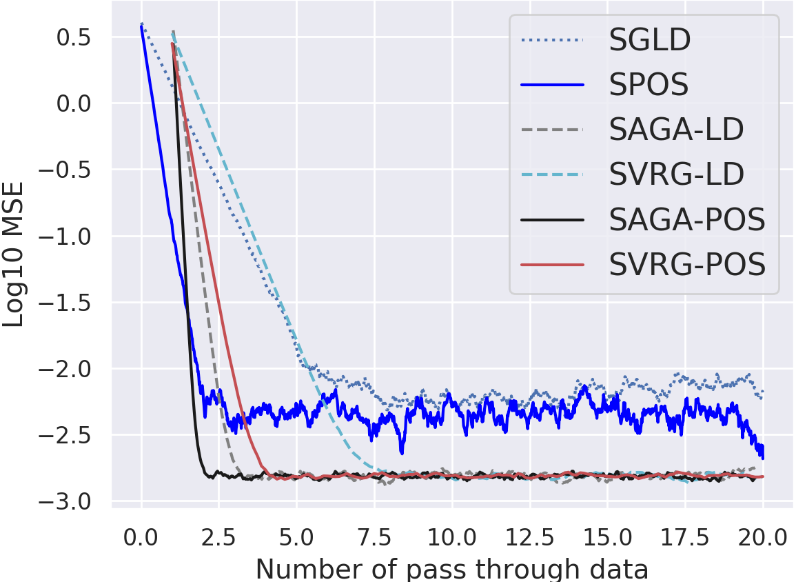
Figure 1: Log-MSE of the mean parameter versus the number of dataset pass.

5.2 Bayesian logistic regression

Following related work such as [9], we test the proposed algorithms for Bayesian-logistic-regression (BLR) on four publicly available datasets from the UCI machine learning repository: $Australian$ (690-14), $Pima$ (768-8), $Diabetic$ (1151-20) and $Susy$ (100000-18), where $(N-d)$ means a dataset of $N$ data points with dimensionality $d$. The first three datasets are relatively small, and the last one is a large dataset suitable to evaluate scalable Bayesian sampling algorithms.

Specifically, consider a dataset $\{X_{i},y_{i}\}_{i=1}^{N}$ with $N$ samples, where $X_{i}\in\mathbb{R}^{d}$ and $y_{i}\in\{0,1\}$. The likelihood of a BLR model is written as $p(y_{i}=1|X_{i},\alpha)=\textsf{sigmoid}(\alpha^{T}X_{i})$ with regression coefficient $\alpha\in\mathbb{R}^{d}$, which is assumed to be sampled from a standard multivariate Gaussian prior $\mathcal{N}(0,I)$ for simplicity. The datasets are split into 80% training data and 20% testing data. Optimized constant stepsizes are applied for each algorithm via grid search. Following existing work, we report testing accuracy and log-likelihood versus the number of data passes for each dataset, averaging over 10 runs with 50 particles. The minibatch size is set to 15 for all experiments.

5.2.1 Variance-reduced SPOS versus SPOS

We first compare SAGA-POS, SVRG-POS and SVRG-POS⁺ with SPOS without variance reduction proposed in [23]. The testing accuracies and log-likelihoods versus number of passes through data on the four datasets are plotted in Figure 2. It is observed that SAGA-POS converges faster than both SVRG-POS and SVRG-POS⁺, all of which outperform SPOS significantly. On the largest dataset SUSY, SAGA-POS starts only after one pass through data, which then converges quickly, outperforming other algorithms. And SVRG-POS⁺ outperforms SVRG-POS due to the dataset SUSY is so large. All of these phenomena are consistent with our theory.

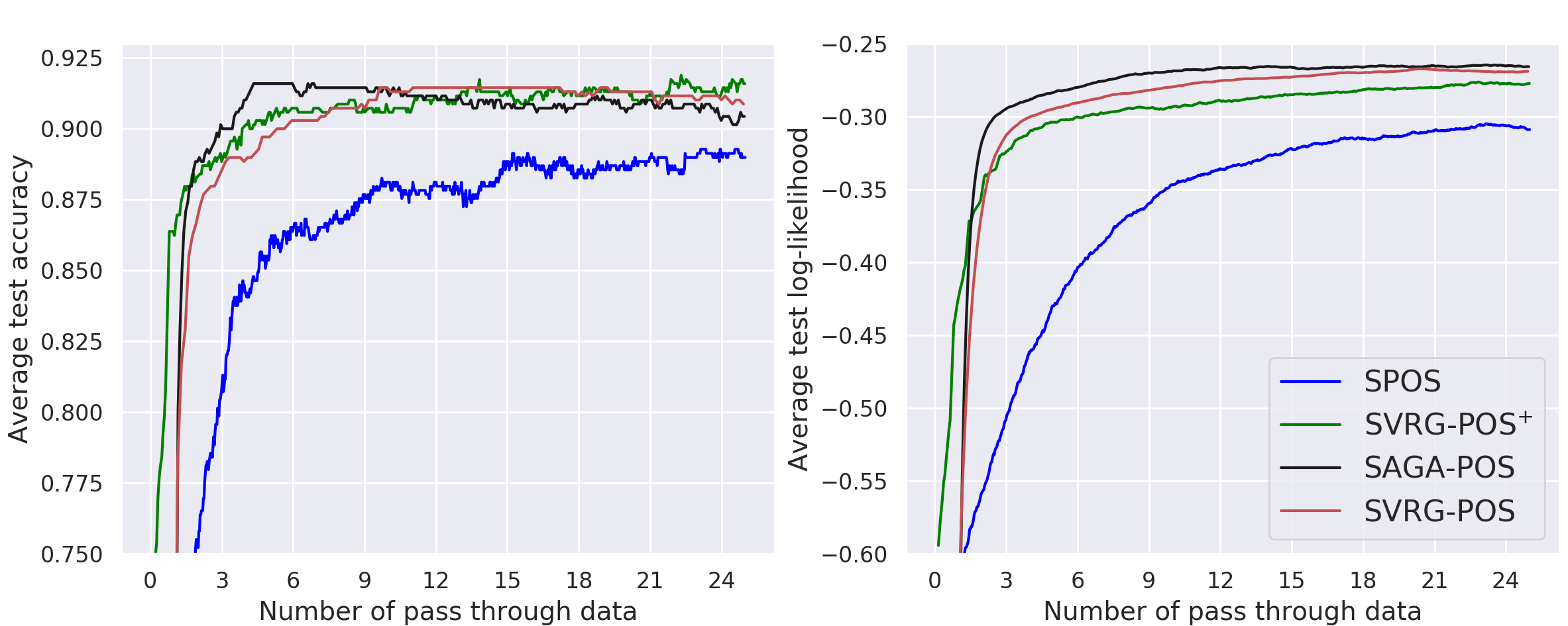
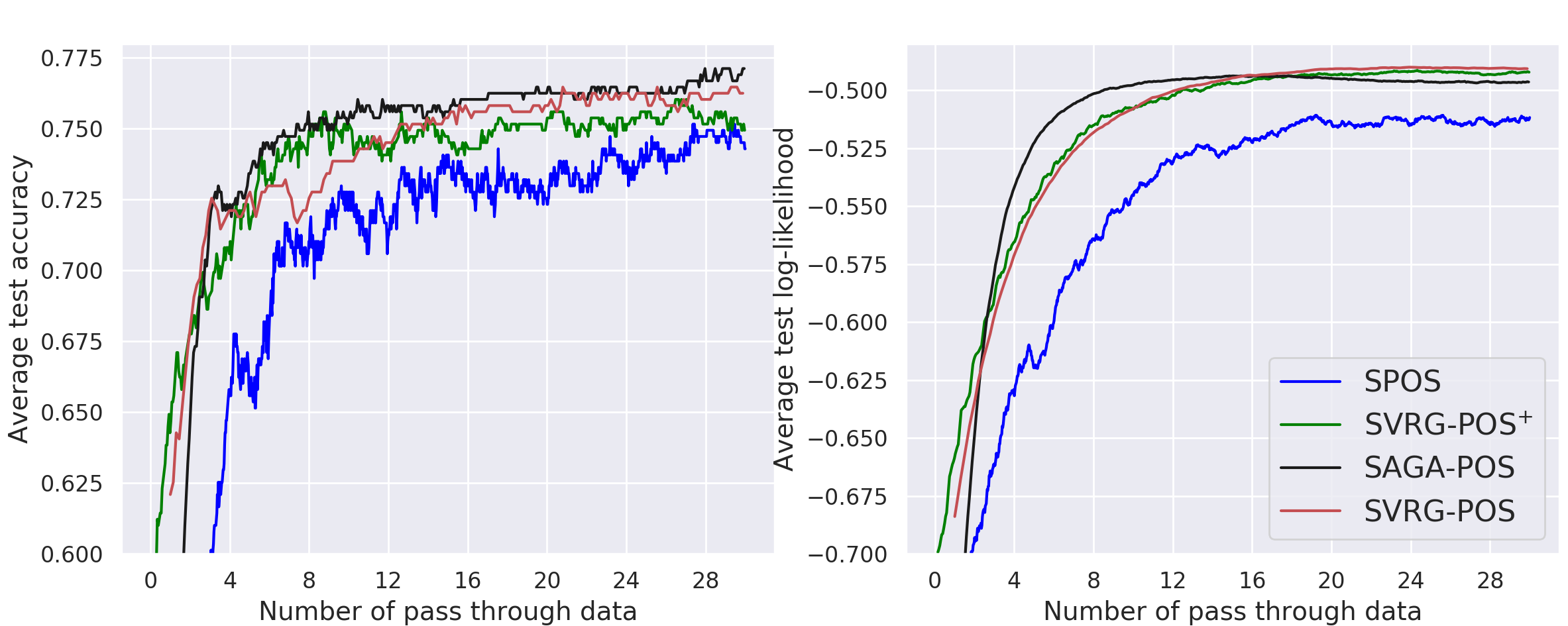
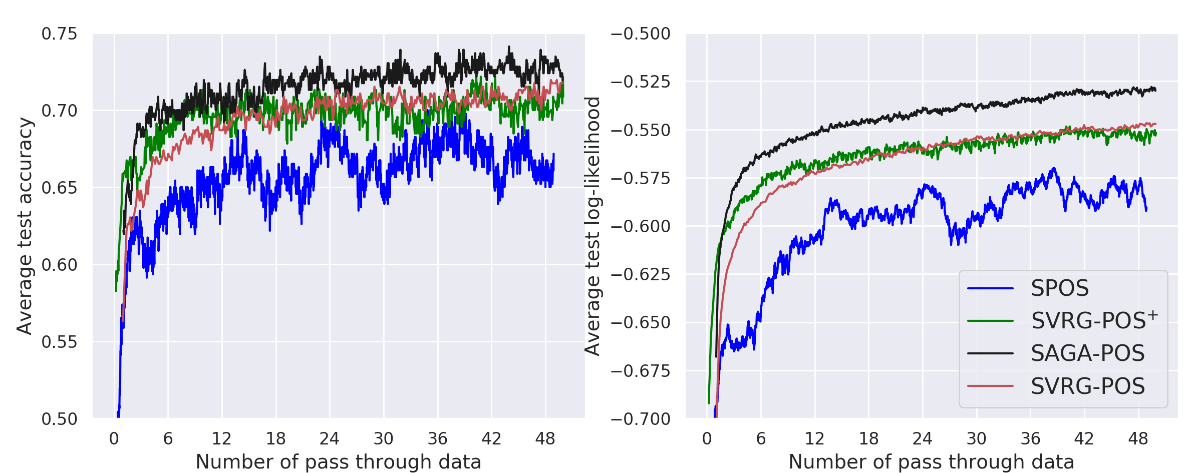
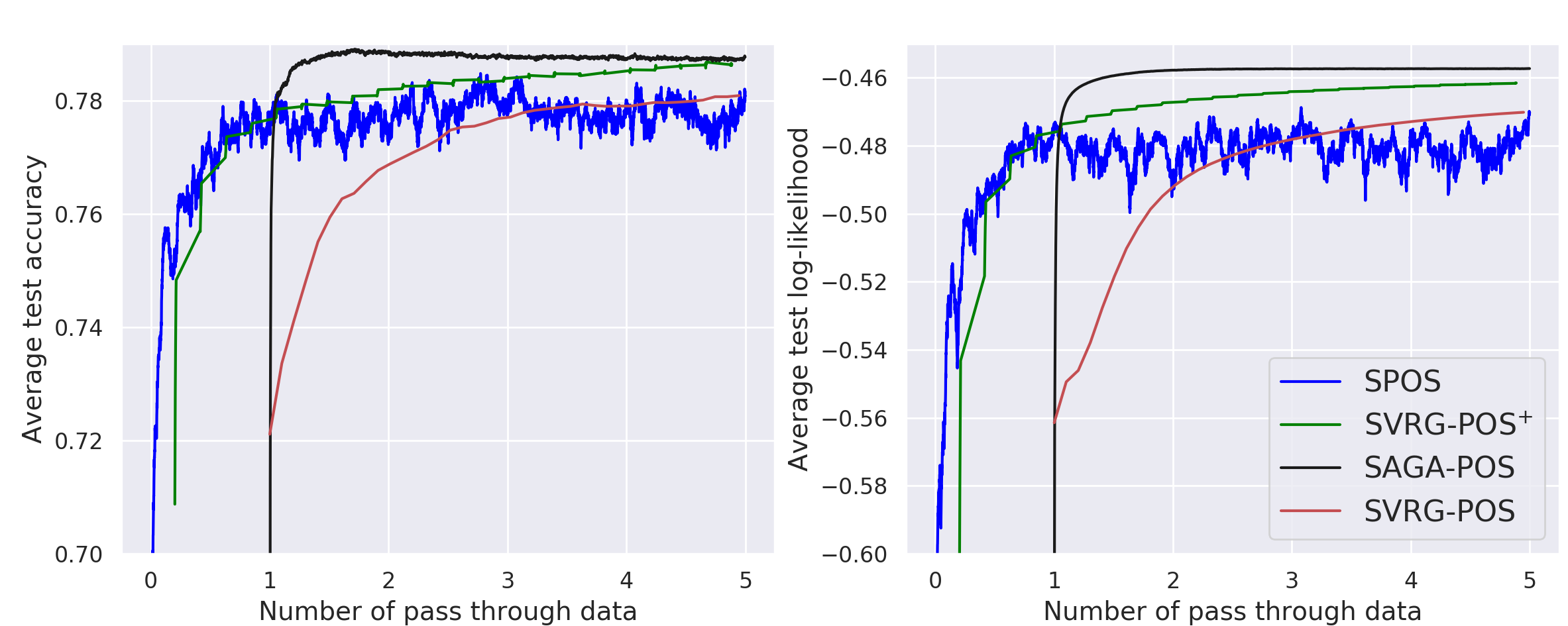
Figure 2: Testing accuracy and log-likelihood vs the number of data pass for SPOS and its variance-reduction variants. From top to bottom: AUSTRALIAN, PIMA, DIABETIC, SUSY datasets.

5.2.2 Variance-reduced SPOS versus variance-reduced SGLD

Next we compare the three variance-reduced SPOS algorithms with its SGLD counterparts, i.e., SAGA-LD, SVRG-LD and SVRG-LD⁺. The results are plotted in Figure 3. Similar phenomena are observed, where both SAGA-POS and SVRG-POS outperform SAGA-LD and SVRG-LD, respectively, consistent with our theoretical results discussed in Remark 3.1 and 3.2. Interestingly, in the PIMA dataset case, SVRG-LD is observed to perform even worse (converge slower) than standard SGLD. Furthermore, as discussed in Remark 4, our theory indicates that the improvement of SVRG-POS over SVRG-LD is more significant than that of SAGA-POS over SAGA-LD. This is indeed true by inspecting the plots in Figure 3.

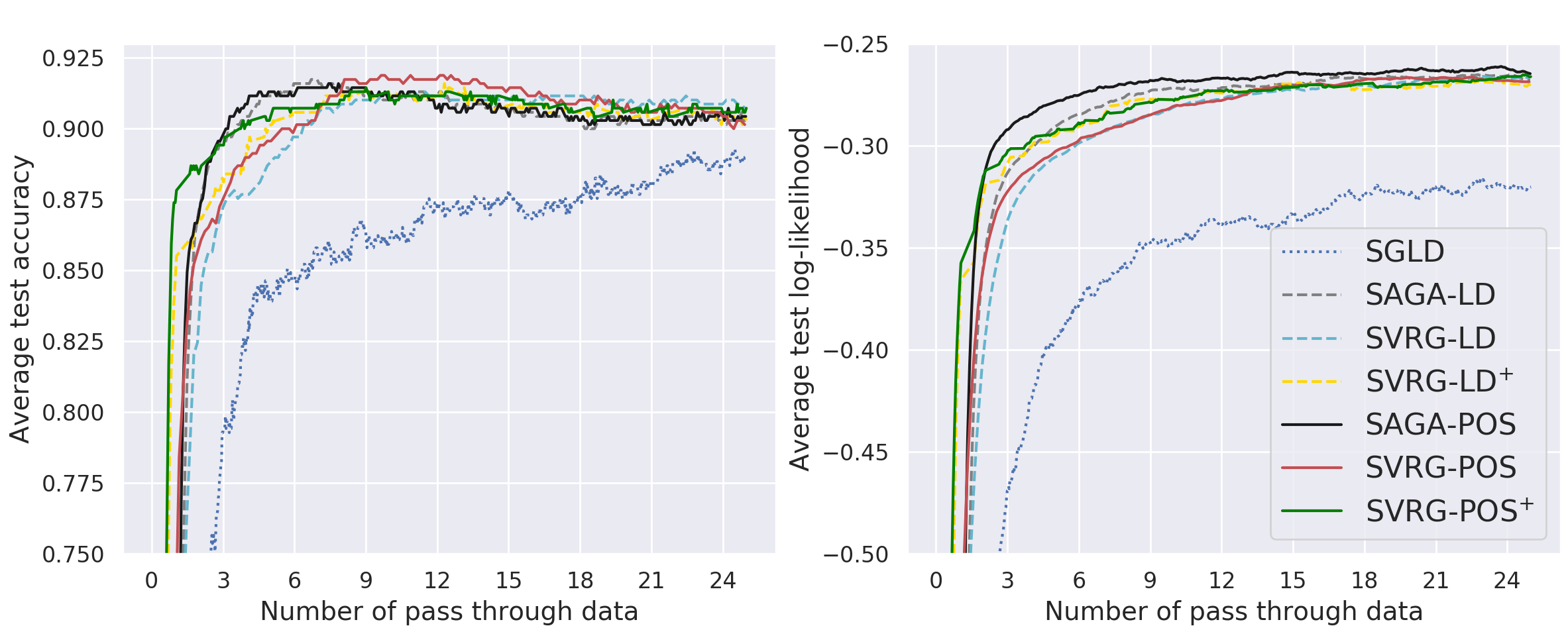
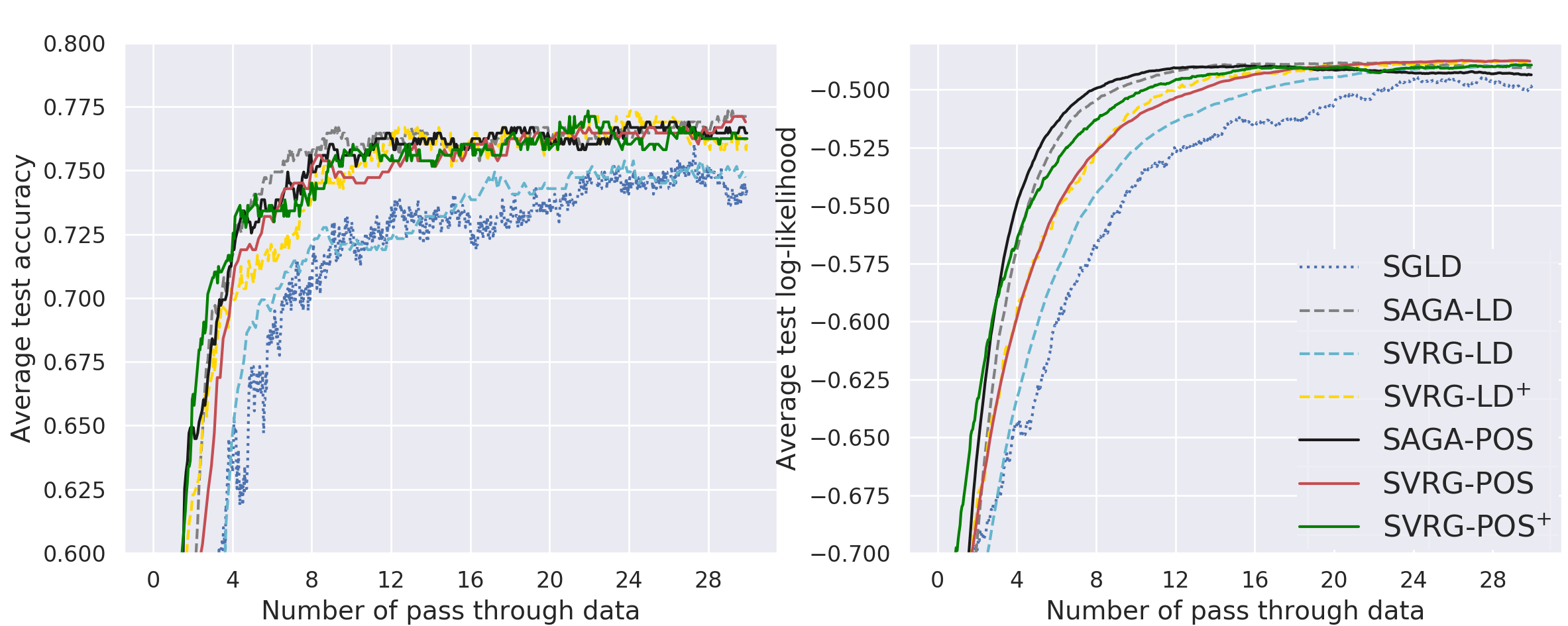
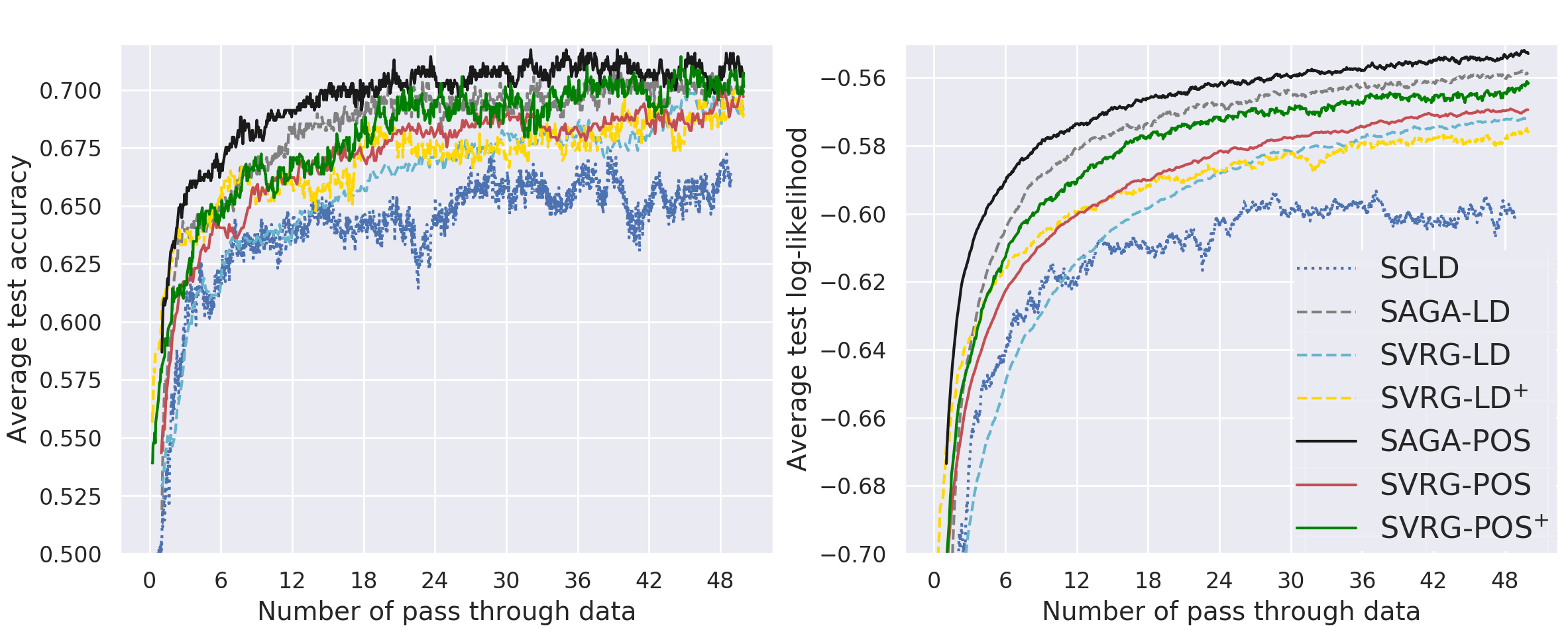
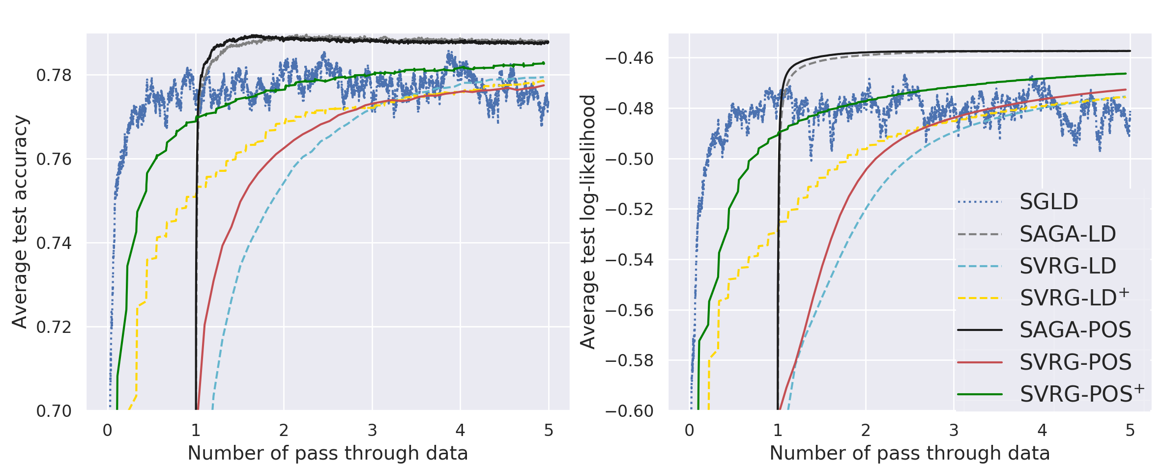
Figure 3: Testing accuracy and log-likelihood versus the number of dataset pass for variance-reduced SPOS and SGLD. From top to bottom: AUSTRALIAN, PIMA, DIABETIC, SUSY datasets.

5.2.3 Impact of number of particles

Finally we examine the impact of number of particles to the convergence rates. As indicated by Theorems 1-3, for a fixed number of iterations $T$, the convergence error in terms of 2-Wasserstein distance decreases with increasing number of particles. To verify this, we run SAGA-POS and SVRG-POS for BLR with the number of particles ranging between $\{1,2,4,8,16\}$. The test log-likelihoods versus iteration numbers are plotted in Figure 4, demonstrating consistency with our theory.

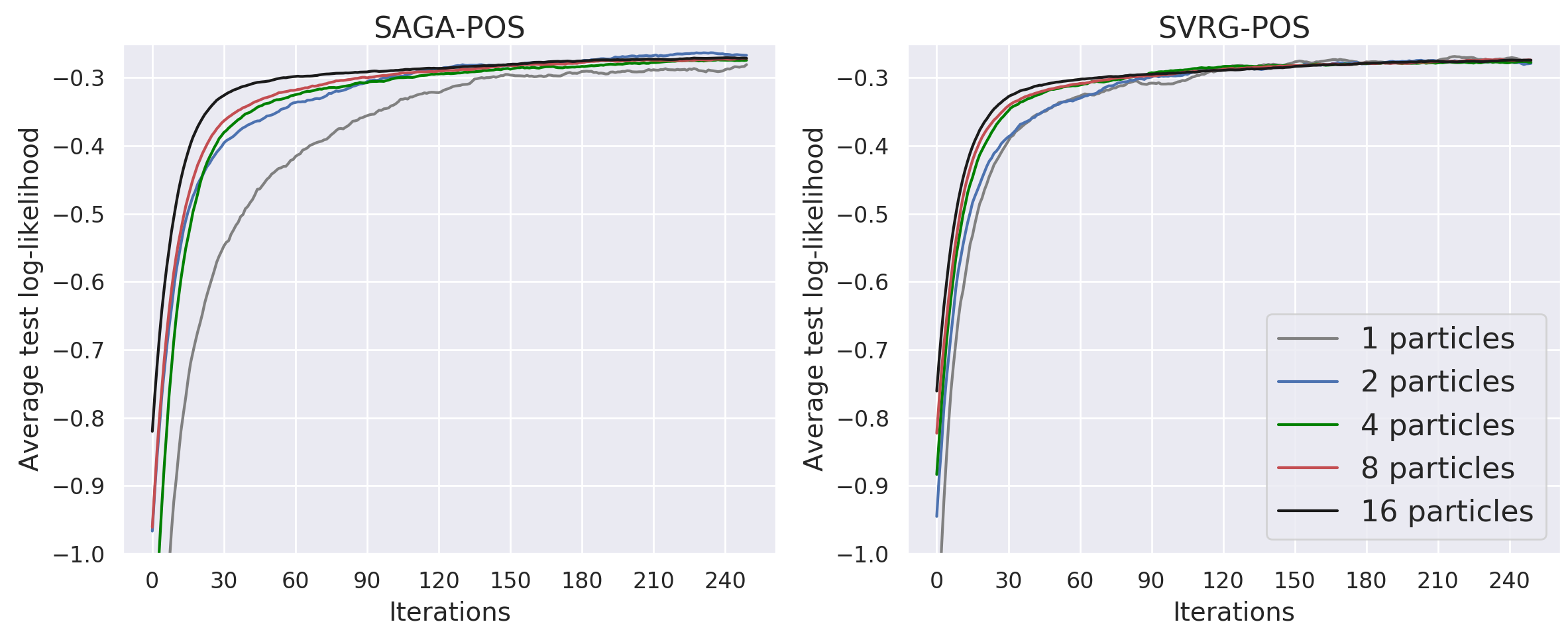
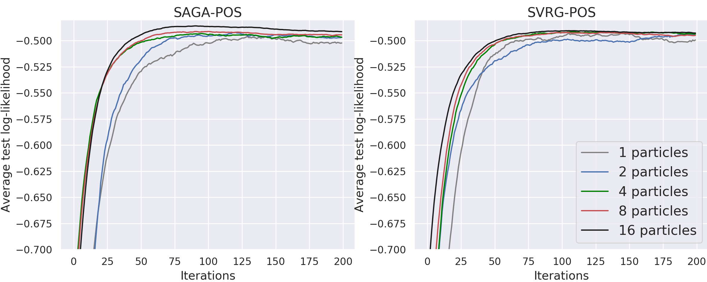
Figure 4: Testing log-likelihood versus number of iterations with different number of particles for variance-reduced SPOS. Top: Australian; Bottom: Pima datasets.

6 Conclusion

We propose several variance-reduction techniques for stochastic particle-optimization sampling, and for the first time, develop nonasymptotic convergence theory for the algorithms in terms of 2-Wasserstein metrics. Our theoretical results indicate the improvement of convergence rates for the proposed variance-reduced SPOS compared to both standard SPOS and the variance-reduced SGLD algorithms. Our theory is verified by a number of experiments on both synthetic data and real data for Bayesian Logistic regression. Leveraging both our theory and empirical findings, we recommend the following algorithm choices in practice: $\textup{\it i})$ SAGA-POS is preferable when storage is not a concern; $\textup{\it ii})$ SVRG-POS is a better choice when storage is a concern and full gradients are feasible to calculate; $\textup{\it iii})$ Otherwise, SVRG-POS⁺ is a good choice and works well in practice.

Appendix A More details about the notations

• If you read this paper carefully, you may notice the different use of ${\bm{\mathchar 28946\relax}}$ and $\mathchar 28946\relax$. ${\bm{\mathchar 28946\relax}}$ is mostly used for the interpretation of the theory. However, $\mathchar 28946\relax$ is only used for the interpretation of algorithms, which means $\mathchar 28946\relax$ often appears with $k$ (which stands for the $k$th interation ) like $\mathchar 28946\relax_{k}$. We design these differences to help you have a better understanding of our results.
  The above rules still apply for the results in Appendix.

• The symbol $\bm{1}(H_{1}\leq H_{2})$ in Theorem 3 means

  $$\bm{1}(H_{1}\leq H_{2})=\begin{cases}1&H_{1}\leq H_{2}\\ 0&H_{1}>H_{2}\end{cases}$$ (13)

  
  

  and the symbol $H_{3}\wedge H_{4}$ means $\min\{H_{3},H_{4}\}$
  

• The relationship between RBF kernel $\kappa({\bm{\mathchar 28946\relax}},{\bm{\mathchar 28946\relax}}^{\prime})=\exp(-\frac{\|{\bm{\mathchar 28946\relax}}-{\bm{\mathchar 28946\relax}}^{\prime}\|^{2}}{2\eta^{2}})$ and the function $K({\bm{\mathchar 28946\relax}})=\exp(-\frac{\|{\bm{\mathchar 28946\relax}}\|^{2}}{2\eta^{2}})$ can be interpreted as $\kappa({\bm{\mathchar 28946\relax}},{\bm{\mathchar 28946\relax}}^{\prime})=K({\bm{\mathchar 28946\relax}}-{\bm{\mathchar 28946\relax}}^{\prime})$ in detail.
  

  We moved the above details about the notations to the appendix due to the space limit.

Appendix B Convergence guarantees for SAGA-LD, SVRG-LD and SVRG-LD⁺

In this section we present the Convergence guarantees for SAGA-LD, SVRG-LD and SVRG-LD+ from [3, 22]

Assumption 4

• (Sum-decomposable) The $F({\bm{\mathchar 28946\relax}})$ is decomposable i.e. $F({\bm{\mathchar 28946\relax}})=\sum_{j=1}^{N}F_{j}({\bm{\mathchar 28946\relax}})$

• (Smoothness) $F({\bm{\mathchar 28946\relax}})$ is Lipschitz continuous with some positive constant, i.e. for all ${\bm{\mathchar 28946\relax}}_{1},{\bm{\mathchar 28946\relax}}_{2}\in\mathbb{R}^{d}$, $\|F({\bm{\mathchar 28946\relax}}_{1})-F({\bm{\mathchar 28946\relax}}_{2})\|\leq L_{F}\left\|{\bm{\mathchar 28946\relax}}_{1}-{\bm{\mathchar 28946\relax}}_{2}\right\|$

• (Strong convexity) $F({\bm{\mathchar 28946\relax}})$ is a $m_{F}$-strongly convex function, i.e. $\left(F({\bm{\mathchar 28946\relax}}_{1})-F({\bm{\mathchar 28946\relax}}_{2})\right)({\bm{\mathchar 28946\relax}}_{1}-{\bm{\mathchar 28946\relax}}_{2})\geq m_{F}\left\|{\bm{\mathchar 28946\relax}}_{1}-{\bm{\mathchar 28946\relax}}_{2}\right\|$

• (Hessian Lischitz) There exits such a positive constant such that $\left\|\nabla F({\bm{\mathchar 28946\relax}}_{1})-\nabla F({\bm{\mathchar 28946\relax}}_{2})\right\|\leq D_{F}\left\|{\bm{\mathchar 28946\relax}}_{1}-{\bm{\mathchar 28946\relax}}_{2}\right\|$

Assumption 5

(Bound Variance) There exits a constant $\sigma\geq 0$, such that for all j

$$\mathbb{E}[\|F_{j}({\bm{\mathchar 28946\relax}})-\frac{1}{N}\sum\limits_{j=1}^{N}F_{j}({\bm{\mathchar 28946\relax}})\|^{2}]\leq d\sigma^{2}/N^{2}$$

Theorem 4

Under Assumption 4, let the step size $h<\frac{B}{8NL_{F}}$ and the batch size $B\geq 9$, then we can have the bound for $\mathcal{W}_{2}(\mu_{T},\mu^{*})$ in the SAGA-LD algorithm

$$\mathcal{W}_{2}(\mu_{T},\mu^{*})\leq 5\exp(-\frac{m_{F}h}{4}T)\mathcal{W}_{2}(\mu_{0},\mu^{*})+$$

$$\frac{2hD_{F}d}{m_{F}}+\frac{2h{L_{F}}^{\frac{3}{2}}\sqrt{d}}{m_{F}}+\frac{24hL_{F}\sqrt{dN}}{\sqrt{m_{F}}B}$$

Theorem 5

Under Assumption 4, if we choose Option $I$ and set the step size $h<\frac{1}{8L_{F}}$, the batch size $B\geq 2$ and the epoch length $\tau\geq\frac{8}{m_{F}h}$, then we can have the bound for all T mod $\tau$ =0 in the SVRG-LD algorithm

$$\mathcal{W}_{2}(\mu_{T},\mu^{*})\leq \exp(-\frac{m_{F}h}{56}T)\frac{\sqrt{L_{F}}}{\sqrt{m_{F}}}\mathcal{W}_{2}(\mu_{0},\mu^{*})+$$

$$\frac{2hD_{F}d}{m_{F}}+\frac{2h{L_{F}}^{\frac{3}{2}}\sqrt{d}}{m_{F}}+\frac{64L_{F}^{\frac{3}{2}}\sqrt{hd}}{m_{F}\sqrt{B}}$$

If we choose Option $II$ and set the step size $h<\frac{\sqrt{B}}{4\tau C_{2}}$, then we can have the bound for all T in the SVRG-LD algorithm

$$\mathcal{W}_{2}(\mu_{T},\mu^{*})\leq \exp(-\frac{m_{F}h}{4}T)\mathcal{W}_{2}(\mu_{0},\mu^{*})+$$

$$\frac{\sqrt{2}hD_{F}d}{m_{F}}+\frac{5h{L_{F}}^{\frac{3}{2}}\sqrt{d}}{m_{F}}+\frac{9hL_{F}\tau\sqrt{d}}{\sqrt{Bm_{F}}}$$

Theorem 6

Under Assumption 4 and Assumption 5, if we set the step size $h\leq min\{(\frac{BC_{3}}{24{C_{2}}^{4}\tau^{2}})^{\frac{1}{3}},\frac{1}{6\tau({C_{5}}^{2}/b+C_{2})}\}$, then we can have the bound for all T in the SVRG-LD⁺ algorithm.

$$\mathcal{W}_{2}(\mu_{T},\mu^{*})\leq(1-hm_{F}/4)^{T}\mathcal{W}_{2}(\mu_{0},\mu^{*})+$$

$$\frac{3\sigma d^{1/2}}{m_{F}b^{1/2}}\bm{1}(b\leq N)+\frac{2hD_{4}d}{m_{F}}+\frac{2h{L_{F}}^{3/2}d^{1/2}}{m_{F}}$$

$$+\frac{4hL_{F}(\tau d)^{1/2}\wedge 3h^{1/2}d^{1/2}\sigma}{\sqrt{Bm_{F}}}$$

Appendix C Proof of the theorems in Section 4

In this section, we give proofs to the theorems in Section 4. We are sorry that the proof of our theorems is a little long since we want to make it more easy to understand. However, this does not affect that fact that our proof is credible. Our proof is based on the idea of [23] and borrow some results from [3, 22]

$$\mathrm{d}{\bm{\mathchar 28946\relax}}_{t}^{(i)}= -\beta^{-1}F({\bm{\mathchar 28946\relax}}_{t}^{(i)})\mathrm{d}t-\frac{1}{M}\sum_{q=1}^{M}K({\bm{\mathchar 28946\relax}}_{t}^{(i)}-{\bm{\mathchar 28946\relax}}_{t}^{(q)})F({\bm{\mathchar 28946\relax}}_{t}^{(q)})\mathrm{d}t$$

$$+\frac{1}{M}\sum_{q=1}^{M}\nabla K({\bm{\mathchar 28946\relax}}_{t}^{(i)}-{\bm{\mathchar 28946\relax}}_{t}^{(q)})\mathrm{d}t+\sqrt{2\beta^{-1}}\mathrm{d}\mathcal{W}_{t}^{(i)}~{}~{}~{}~{}\forall i~{}$$ (14)

As mention is Section 2.3 we denote the distribution of ${\bm{\mathchar 28946\relax}}_{t}^{(i)}$ in Eq.(C) as $\nu_{t}$. From the proof of Theorem 3 and Remark 1 in [23] we can derive that

$$\mathcal{W}_{2}(\nu_{\infty},\mu^{*})\leq\frac{H_{\nabla K}+H_{F}}{\sqrt{2M}(\beta^{-1}-3H_{F}L_{K}-2L_{F})}$$ (15)

In order to bound $\mathcal{W}_{2}(\mu_{T},\mu^{*})$, we need to bound $\mathcal{W}_{2}(\mu_{T},\nu_{\infty})$ next. Now we borrow the idea in [23] , concatenating the particles at each time into a single vector representation, We define a new parameter at time $t$ as ${\bm{\mathchar 28930\relax}}_{t}\triangleq[{\bm{\mathchar 28946\relax}}_{t}^{(1)},\cdots,{\bm{\mathchar 28946\relax}}_{t}^{(M)}]\in\mathbb{R}^{Md}$. Consequently, ${\bm{\mathchar 28930\relax}}_{t}$ is driven by the following linear SDE:

$$\mathrm{d}{\bm{\mathchar 28930\relax}}_{t}=-F^{{\bm{\mathchar 28930\relax}}}({\bm{\mathchar 28930\relax}}_{t})\mathrm{d}t+\sqrt{2\beta^{-1}}\mathrm{d}\mathcal{W}_{t}^{(Md)}~{},$$ (16)

$F^{{\bm{\mathchar 28930\relax}}}({\bm{\mathchar 28930\relax}}_{t})\triangleq[\beta^{-1}F({\bm{\mathchar 28946\relax}}_{t}^{(1)})-\frac{1}{M}\sum_{q=1}^{M}\nabla K({\bm{\mathchar 28946\relax}}_{t}^{(1)}-{\bm{\mathchar 28946\relax}}_{t}^{(q)})\\ +\frac{1}{M}\sum_{q=1}^{M}K({\bm{\mathchar 28946\relax}}_{t}^{(1)}-{\bm{\mathchar 28946\relax}}_{t}^{(q)})F({\bm{\mathchar 28946\relax}}_{t}^{(q)}),\cdots,\beta^{-1}F({\bm{\mathchar 28946\relax}}_{t}^{(M)})-\frac{1}{M}\sum_{q=1}^{M}\nabla K({\bm{\mathchar 28946\relax}}_{t}^{(M)}-{\bm{\mathchar 28946\relax}}_{t}^{(q)})+\frac{1}{M}\sum_{q=1}^{M}K({\bm{\mathchar 28946\relax}}_{t}^{(M)}-{\bm{\mathchar 28946\relax}}_{t}^{(q)})F({\bm{\mathchar 28946\relax}}_{t}^{(q)})]$ is a vector function $\mathbb{R}^{Md}\rightarrow\mathbb{R}^{Md}$, and $\mathcal{W}_{t}^{(Md)}$ is Brownian motion of dimension $Md$.

Now we define the $F^{{\bm{\mathchar 28930\relax}}}_{j}({\bm{\mathchar 28930\relax}}_{t})\triangleq[\beta^{-1}F_{j}({\bm{\mathchar 28946\relax}}_{t}^{(1)})-\frac{1}{MN}\sum_{q=1}^{M}\nabla K({\bm{\mathchar 28946\relax}}_{t}^{(1)}-{\bm{\mathchar 28946\relax}}_{t}^{(q)})+\frac{1}{M}\sum_{q=1}^{M}K({\bm{\mathchar 28946\relax}}_{t}^{(1)}-{\bm{\mathchar 28946\relax}}_{t}^{(q)})F_{j}({\bm{\mathchar 28946\relax}}_{t}^{(q)}),\cdots,\beta^{-1}F_{j}({\bm{\mathchar 28946\relax}}_{t}^{(M)})-\frac{1}{MN}\sum_{q=1}^{M}\nabla K({\bm{\mathchar 28946\relax}}_{t}^{(M)}\\ -{\bm{\mathchar 28946\relax}}_{t}^{(q)})+\frac{1}{M}\sum_{q=1}^{M}K({\bm{\mathchar 28946\relax}}_{t}^{(M)}-{\bm{\mathchar 28946\relax}}_{t}^{(q)})F_{j}({\bm{\mathchar 28946\relax}}_{t}^{(q)})]$. We can find the $F^{{\bm{\mathchar 28930\relax}}}{({\bm{\mathchar 28930\relax}}_{t})}$ and $F^{{\bm{\mathchar 28930\relax}}}_{j}({\bm{\mathchar 28930\relax}}_{t})$ defined above satisfy the following theorem.

Theorem 7

• (Sum-decomposable) The $F^{{\bm{\mathchar 28930\relax}}}({\bm{\mathchar 28930\relax}})$ is decomposable i.e. $F^{{\bm{\mathchar 28930\relax}}}({\bm{\mathchar 28930\relax}})=\sum_{j=1}^{N}F^{{\bm{\mathchar 28930\relax}}}_{j}({\bm{\mathchar 28930\relax}})$

• (Smoothness) $F^{{\bm{\mathchar 28930\relax}}}$ is Lipschitz continuous with some positive constant, i.e. for all ${\bm{\mathchar 28930\relax}}_{1},{\bm{\mathchar 28930\relax}}_{2}\in\mathbb{R}^{Md}$,$\|F^{{\bm{\mathchar 28930\relax}}}({\bm{\mathchar 28930\relax}}_{1})-F^{{\bm{\mathchar 28930\relax}}}({\bm{\mathchar 28930\relax}}_{2})\|\leq\sqrt{2(\beta^{-1}L_{F}+2L_{K}H_{F}+H_{K}L_{F}+L_{\nabla K})^{2}+2}\left\|{\bm{\mathchar 28930\relax}}_{1}-{\bm{\mathchar 28930\relax}}_{2}\right\|$

• (Strong convexity) $F^{{\bm{\mathchar 28930\relax}}}$ is a $(\beta^{-1}m_{F}--2L_{F}-3H_{F}L_{K})$-strongly convex function, i.e. $\left(F^{{\bm{\mathchar 28930\relax}}}({\bm{\mathchar 28930\relax}}_{1})-F^{{\bm{\mathchar 28930\relax}}}({\bm{\mathchar 28930\relax}}_{2})\right)({\bm{\mathchar 28930\relax}}_{1}-{\bm{\mathchar 28930\relax}}_{2})\leq(\beta^{-1}m_{F}-2L_{F}-3H_{F}L_{K})\left\|{\bm{\mathchar 28930\relax}}_{1}-{\bm{\mathchar 28930\relax}}_{2}\right\|$

• (Hessian Lischitz) The function $F^{{\bm{\mathchar 28930\relax}}}$ is Hessian Lipschitz, i.e., $\left\|\nabla F^{{\bm{\mathchar 28930\relax}}}({\bm{\mathchar 28930\relax}}_{1})-\nabla F^{{\bm{\mathchar 28930\relax}}}({\bm{\mathchar 28930\relax}}_{2})\right\|\leq(\beta^{-1}D_{F}+4D_{\nabla^{2}K}+4H_{F}L_{\nabla K}+2L_{F}H_{\nabla K}+2H_{F}L_{K}+L_{F}H_{K})\left\|{\bm{\mathchar 28930\relax}}_{1}-{\bm{\mathchar 28930\relax}}_{2}\right\|$

• (Bound Variance) There exits a constant, $\sigma\geq 0$, such that for all $j$,

  $$\mathbb{E}[\|F^{{\bm{\mathchar 28930\relax}}}_{j}({\bm{\mathchar 28930\relax}})-\frac{1}{N}\sum\limits_{j=1}^{N}F^{{\bm{\mathchar 28930\relax}}}_{j}({\bm{\mathchar 28930\relax}})\|^{2}]\leq Md(2\beta^{-1}+2H_{K}^{2})\sigma^{2}/N^{2}$$

• • The sum-decomposable property of $F^{{\bm{\mathchar 28930\relax}}}({\bm{\mathchar 28930\relax}})$ is easy to verify. And the smoothness property of $F^{{\bm{\mathchar 28930\relax}}}$ can be derived directly from the proof of the Lemma 13 in [23].

  • (Strong convexity)

    $$(F^{{\bm{\mathchar 28930\relax}}}({\bm{\mathchar 28930\relax}}_{1})-F^{{\bm{\mathchar 28930\relax}}}({\bm{\mathchar 28930\relax}}_{2}))({\bm{\mathchar 28930\relax}}_{1}-{\bm{\mathchar 28930\relax}}_{2})=$$ (17)

    $$\frac{1}{M}\sum_{i,q}^{M}(\xi_{iq}^{1}+\xi_{iq}^{2}+\xi_{iq}^{3}+\xi_{iq}^{4})$$

    where

    $$\xi_{iq}^{1}=\beta^{-1}\left(F({\bm{\mathchar 28946\relax}}_{1}^{(i)})-F({{\bm{\mathchar 28946\relax}}}_{2}^{(i)})\right)\cdot\left({\bm{\mathchar 28946\relax}}_{1}^{(i)}-{{\bm{\mathchar 28946\relax}}}_{2}^{(i)}\right)$$

    $$\xi_{iq}^{2}=-\left(\nabla K({\bm{\mathchar 28946\relax}}_{1}^{(i)}-{\bm{\mathchar 28946\relax}}_{1}^{(q)})-\nabla K({\bm{\mathchar 28946\relax}}_{2}^{(i)}-{\bm{\mathchar 28946\relax}}_{2}^{(q)})\right)\cdot\left({\bm{\mathchar 28946\relax}}_{1}^{(i)}-{\bm{\mathchar 28946\relax}}_{2}^{(i)}\right)$$

    $$\xi_{iq}^{3}=\left(F({\bm{\mathchar 28946\relax}}_{1}^{(q)})K({\bm{\mathchar 28946\relax}}_{1}^{(i)}-{\bm{\mathchar 28946\relax}}_{1}^{(q)})-F({\bm{\mathchar 28946\relax}}_{2}^{(q)})K({\bm{\mathchar 28946\relax}}_{1}^{(i)}-{\bm{\mathchar 28946\relax}}_{1}^{(q)})\right)\cdot$$

    $$\left({\bm{\mathchar 28946\relax}}_{1}^{(i)}-{{\bm{\mathchar 28946\relax}}}_{2}^{(i)}\right)$$

    $$\xi_{iq}^{4}=\left(F({\bm{\mathchar 28946\relax}}_{2}^{(q)})K({\bm{\mathchar 28946\relax}}_{1}^{(i)}-{\bm{\mathchar 28946\relax}}_{1}^{(q)})-F({\bm{\mathchar 28946\relax}}_{2}^{(q)})K({\bm{\mathchar 28946\relax}}_{2}^{(i)}-{\bm{\mathchar 28946\relax}}_{2}^{(q)})\right)\cdot$$

    $$\left({\bm{\mathchar 28946\relax}}_{1}^{(i)}-{{\bm{\mathchar 28946\relax}}}_{2}^{(i)}\right)$$

    For the $\xi_{iq}^{1}$ terms, applying the convex condition for $F$, we have

    $$\sum_{iq}\xi_{iq}^{1} =\sum_{iq}\beta^{-1}\left(F({\bm{\mathchar 28946\relax}}_{1}^{(i)})-F({{\bm{\mathchar 28946\relax}}}_{2}^{(i)}\right)\cdot\left({\bm{\mathchar 28946\relax}}_{1}^{(i)}-{{\bm{\mathchar 28946\relax}}}_{2}^{(i)}\right)$$

    $$\geq\beta^{-1}m_{F}M\sum_{i}\left\|{\bm{\mathchar 28946\relax}}_{1}^{(i)}-{{\bm{\mathchar 28946\relax}}}_{2}^{(i)}\right\|^{2}$$ (18)

    For the $\xi_{iq}^{2}$ term, applying the concave condition for $W$ and $\nabla W$ is odd, we have $\sum_{iq}\xi_{iq}^{2}=-$

    $$\sum_{iq}^{M}\left(\nabla K({\bm{\mathchar 28946\relax}}_{1}^{(i)}-{\bm{\mathchar 28946\relax}}_{1}^{(q)})-\nabla K({\bm{\mathchar 28946\relax}}_{2}^{(i)}-{\bm{\mathchar 28946\relax}}_{2}^{(q)})\right)\cdot\left({\bm{\mathchar 28946\relax}}_{1}^{(i)}-{\bm{\mathchar 28946\relax}}_{2}^{(i)}\right)$$

    $$= -\frac{1}{2}\sum_{iq}^{M}\sum_{iq}^{M}\left(\nabla K({\bm{\mathchar 28946\relax}}_{1}^{(i)}-{\bm{\mathchar 28946\relax}}_{1}^{(q)})-\nabla K({\bm{\mathchar 28946\relax}}_{2}^{(i)}-{\bm{\mathchar 28946\relax}}_{2}^{(q)})\right)$$

    $$\cdot\left({\bm{\mathchar 28946\relax}}_{1}^{(i)}-{\bm{\mathchar 28946\relax}}_{1}^{(q)}-({\bm{\mathchar 28946\relax}}_{2}^{(i)}-{\bm{\mathchar 28946\relax}}_{2}^{(q)})\right)$$

    $$\geq\frac{1}{2}m_{K}\sum_{iq}^{M}\left\|{\bm{\mathchar 28946\relax}}_{1}^{(i)}-{\bm{\mathchar 28946\relax}}_{1}^{(q)}-({\bm{\mathchar 28946\relax}}_{2}^{(i)}-{\bm{\mathchar 28946\relax}}_{2}^{(q)})\right\|^{2}\geq 0$$ (19)

    For the $\xi_{iq}^{3}$ terms, after applying the $L_{F}$-Lipschitz property of $F$, we have $\sum_{iq}\xi_{iq}^{3}=$

    $$\sum_{iq}(F({\bm{\mathchar 28946\relax}}_{1}^{(q)})K({\bm{\mathchar 28946\relax}}_{1}^{(i)}-{\bm{\mathchar 28946\relax}}_{1}^{(q)})-F({\bm{\mathchar 28946\relax}}_{2}^{(q)})K({\bm{\mathchar 28946\relax}}_{1}^{(i)}-{\bm{\mathchar 28946\relax}}_{1}^{(q)}))$$

    $$\cdot\left({\bm{\mathchar 28946\relax}}_{1}^{(i)}-{\bm{\mathchar 28946\relax}}_{2}^{(i)}\right)\geq-\sum_{iq}L_{F}\left\|{\bm{\mathchar 28946\relax}}_{1}^{(q)}-{\bm{\mathchar 28946\relax}}_{2}^{(q)}\right\|\left\|{\bm{\mathchar 28946\relax}}_{1}^{(i)}-{\bm{\mathchar 28946\relax}}_{2}^{(i)}\right\|$$

    $$\geq-2L_{F}M\sum_{i}\left\|{\bm{\mathchar 28946\relax}}_{1}^{(i)}-{\bm{\mathchar 28946\relax}}_{2}^{(i)}\right\|^{2}~{}\$$ (20)

    For the $\xi_{iq}^{4}$ terms, we have $\sum_{iq}\xi_{iq}^{4}=$

    $$\sum_{iq}(F({\bm{\mathchar 28946\relax}}_{2}^{(q)})K({\bm{\mathchar 28946\relax}}_{1}^{(i)}-{\bm{\mathchar 28946\relax}}_{1}^{(q)})-F({\bm{\mathchar 28946\relax}}_{2}^{(q)})K({\bm{\mathchar 28946\relax}}_{2}^{(i)}-{\bm{\mathchar 28946\relax}}_{2}^{(q)}))$$

    $$\cdot\left({\bm{\mathchar 28946\relax}}_{1}^{(i)}-{{\bm{\mathchar 28946\relax}}}_{2}^{(i)}\right)$$

    $$\geq-H_{F}L_{K}\sum_{iq}\left\|{\bm{\mathchar 28946\relax}}_{1}^{(i)}-{\bm{\mathchar 28946\relax}}_{1}^{(q)}-({\bm{\mathchar 28946\relax}}_{2}^{(i)}-{\bm{\mathchar 28946\relax}}_{2}^{(q)})\right\|\left\|{\bm{\mathchar 28946\relax}}_{1}^{(i)}-{\bm{\mathchar 28946\relax}}_{2}^{(i)}\right\|$$

    $$\geq-3H_{F}L_{K}M\sum_{i}\left\|{\bm{\mathchar 28946\relax}}_{1}^{(i)}-{\bm{\mathchar 28946\relax}}_{2}^{(i)}\right\|^{2}$$ (21)

    Then we finally arrive at:

    $$\left(F^{{\bm{\mathchar 28930\relax}}}({\bm{\mathchar 28930\relax}}_{1})-F^{{\bm{\mathchar 28930\relax}}}({\bm{\mathchar 28930\relax}}_{2})\right)({\bm{\mathchar 28930\relax}}_{1}-{\bm{\mathchar 28930\relax}}_{2})$$

    $$\geq(\beta^{-1}m_{F}-2L_{F}-3H_{F}L_{K})\sum_{i}\left\|{\bm{\mathchar 28946\relax}}_{1}^{(i)}-{\bm{\mathchar 28946\relax}}_{2}^{(i)}\right\|$$

    $$\geq(\beta^{-1}m_{F}-2L_{F}-3H_{F}L_{K})\left\|{\bm{\mathchar 28930\relax}}_{1}-{\bm{\mathchar 28930\relax}}_{2}\right\|$$ (22)

  • Now, we will prove the fourth result:

    $$\left\|\nabla F^{{\bm{\mathchar 28930\relax}}}({\bm{\mathchar 28930\relax}}_{1})-\nabla F^{{\bm{\mathchar 28930\relax}}}({\bm{\mathchar 28930\relax}}_{2})\right\|$$

    $$\leq\beta^{-1}\sum_{i=1}^{M}\left\|\nabla F({\bm{\mathchar 28946\relax}}_{1}^{(i)})-\nabla F({\bm{\mathchar 28946\relax}}_{2}^{(i)})\right\|+\sum_{i=1}^{M}\frac{2}{M}\sum_{q=1}^{M}\left\|\nabla^{2}K({\bm{\mathchar 28946\relax}}_{1}^{(i)}-{\bm{\mathchar 28946\relax}}_{1}^{(q)})-\nabla^{2}K({\bm{\mathchar 28946\relax}}_{2}^{(i)}-{\bm{\mathchar 28946\relax}}_{2}^{(q)})\right\|+$$

    $$\frac{2}{M}\sum_{i=1}^{M}\sum_{q=1}^{M}\|\nabla K({\bm{\mathchar 28946\relax}}_{1}^{(i)}-{\bm{\mathchar 28946\relax}}_{1}^{(q)})F({\bm{\mathchar 28946\relax}}_{1}^{(q)})-\nabla K({\bm{\mathchar 28946\relax}}_{2}^{(i)}-{\bm{\mathchar 28946\relax}}_{2}^{(q)})F({\bm{\mathchar 28946\relax}}_{2}^{(q)})\|$$

    $$+\sum_{i=1}^{M}\sum_{q=1}^{M}\frac{1}{M}\|K({\bm{\mathchar 28946\relax}}_{1}^{(i)}-{\bm{\mathchar 28946\relax}}_{1}^{(q)})\nabla F({\bm{\mathchar 28946\relax}}_{1}^{(q)})-K({\bm{\mathchar 28946\relax}}_{2}^{(i)}-{\bm{\mathchar 28946\relax}}_{2}^{(q)})\nabla F({\bm{\mathchar 28946\relax}}_{2}^{(q)})\|$$

    $$\leq\sum_{i=1}^{M}\beta^{-1}D_{F}\|{\bm{\mathchar 28946\relax}}_{1}^{(i)}-{\bm{\mathchar 28946\relax}}_{2}^{(i)}\|+4D_{\nabla^{2}K}\sum_{i=1}^{M}\|{\bm{\mathchar 28946\relax}}_{1}^{(i)}-{\bm{\mathchar 28946\relax}}_{2}^{(i)}\|+$$

    $$\frac{2}{M}\sum_{i=1}^{M}\sum_{q=1}^{M}\|\nabla K({\bm{\mathchar 28946\relax}}_{1}^{(i)}-{\bm{\mathchar 28946\relax}}_{1}^{(q)})F({\bm{\mathchar 28946\relax}}_{1}^{(q)})-\nabla K({\bm{\mathchar 28946\relax}}_{2}^{(i)}-{\bm{\mathchar 28946\relax}}_{2}^{(q)})F({\bm{\mathchar 28946\relax}}_{1}^{(q)})\|+$$

    $$\frac{2}{M}\sum_{i=1}^{M}\sum_{q=1}^{M}\|\nabla K({\bm{\mathchar 28946\relax}}_{2}^{(i)}-{\bm{\mathchar 28946\relax}}_{2}^{(q)})F({\bm{\mathchar 28946\relax}}_{1}^{(q)})-\nabla K({\bm{\mathchar 28946\relax}}_{2}^{(i)}-{\bm{\mathchar 28946\relax}}_{2}^{(q)})F({\bm{\mathchar 28946\relax}}_{2}^{(q)})\|$$

    $$+\frac{1}{M}\sum_{i=1}^{M}\sum_{q=1}^{M}\|K({\bm{\mathchar 28946\relax}}_{1}^{(i)}-{\bm{\mathchar 28946\relax}}_{1}^{(q)})F({\bm{\mathchar 28946\relax}}_{1}^{(q)})-K({\bm{\mathchar 28946\relax}}_{2}^{(i)}-{\bm{\mathchar 28946\relax}}_{2}^{(q)})F({\bm{\mathchar 28946\relax}}_{1}^{(q)})\|+$$

    $$\frac{1}{M}\sum_{i=1}^{M}\sum_{q=1}^{M}\|K({\bm{\mathchar 28946\relax}}_{2}^{(i)}-{\bm{\mathchar 28946\relax}}_{2}^{(q)})F({\bm{\mathchar 28946\relax}}_{1}^{(q)})-K({\bm{\mathchar 28946\relax}}_{2}^{(i)}-{\bm{\mathchar 28946\relax}}_{2}^{(q)})F({\bm{\mathchar 28946\relax}}_{2}^{(q)})\|$$

    $$\leq\sum_{i=1}^{M}\beta^{-1}D_{F}\left\|{\bm{\mathchar 28946\relax}}_{1}^{(i)}-{\bm{\mathchar 28946\relax}}_{2}^{(i)}\right\|+4D_{\nabla^{2}K}\sum_{i=1}^{M}\left\|{\bm{\mathchar 28946\relax}}_{1}^{(i)}-{\bm{\mathchar 28946\relax}}_{2}^{(i)}\right\|+$$

    $$4\sum_{i=1}^{M}H_{F}L_{\nabla K}\left\|{\bm{\mathchar 28946\relax}}_{1}^{(i)}-{\bm{\mathchar 28946\relax}}_{2}^{(i)}\right\|+2\sum_{i=1}^{M}L_{F}H_{\nabla K}\left\|{\bm{\mathchar 28946\relax}}_{1}^{(i)}-{\bm{\mathchar 28946\relax}}_{2}^{(i)}\right\|+$$

    $$2\sum_{i=1}^{M}H_{F}L_{K}\left\|{\bm{\mathchar 28946\relax}}_{1}^{(i)}-{\bm{\mathchar 28946\relax}}_{2}^{(i)}\right\|+\sum_{i=1}^{M}L_{F}H_{K}\left\|{\bm{\mathchar 28946\relax}}_{1}^{(i)}-{\bm{\mathchar 28946\relax}}_{2}^{(i)}\right\|$$

    $$\leq(\beta^{-1}D_{F}+4D_{\nabla^{2}K}+4H_{F}L_{\nabla K}+2L_{F}H_{\nabla K}+$$

    $$2H_{F}L_{K}+L_{F}H_{K})\left\|{\bm{\mathchar 28930\relax}}_{1}-{\bm{\mathchar 28930\relax}}_{2}\right\|$$ (23)

  • Now, we will prove the last result.

    $$\mathbb{E}[\|F^{{\bm{\mathchar 28930\relax}}}_{j}({\bm{\mathchar 28930\relax}})-\frac{1}{N}\sum\limits_{j=1}^{N}F^{{\bm{\mathchar 28930\relax}}}_{j}({\bm{\mathchar 28930\relax}})\|^{2}]=$$

    $$\sum_{i=1}^{M}\mathbb{E}[\|\beta^{-1}F_{j}({\bm{\mathchar 28946\relax}}^{(i)})-\beta^{-1}\frac{1}{N}\sum\limits_{j=1}^{N}F_{j}({\bm{\mathchar 28946\relax}}^{(i)})$$

    $$+\frac{1}{M}\sum_{q=1}^{M}K({\bm{\mathchar 28946\relax}}^{(i)}-{\bm{\mathchar 28946\relax}}^{(q)})F_{j}({\bm{\mathchar 28946\relax}}_{t}^{(q)})-$$

    $$\frac{1}{MN}\sum_{j=1}^{N}\sum_{q=1}^{M}K({\bm{\mathchar 28946\relax}}^{(i)}-{\bm{\mathchar 28946\relax}}^{(q)})F_{j}({\bm{\mathchar 28946\relax}}_{t}^{(q)})\|^{2}]$$

    $$\leq\sum_{i=1}^{M}[2\mathbb{E}\|\beta^{-1}F_{j}({\bm{\mathchar 28946\relax}}^{(i)})-\beta^{-1}\frac{1}{N}\sum\limits_{j=1}^{N}F_{j}({\bm{\mathchar 28946\relax}}^{(i)})\|^{2}$$

    $$+2\frac{H_{K}^{2}}{M^{2}}\mathbb{E}\|\sum_{q=1}^{M}\left(F_{j}({\bm{\mathchar 28946\relax}}^{(q)}-\frac{1}{N}\sum_{j=1}^{N}F_{j}({\bm{\mathchar 28946\relax}}^{(q)})\right)\|^{2}]$$

    $$\leq\sum_{i=1}^{M}({2d\sigma^{2}+2H_{K}^{2}d\sigma^{2}})/N^{2}$$

    $$\leq Md(2\sigma^{2}+2H_{K}^{2}\sigma^{2})/N^{2}$$ (24)

We apply Euler-Maruyama discretization to Eq.(16) and substitute $G_{k}^{\mathchar 28930\relax}$ for $F^{\mathchar 28930\relax}(\mathchar 28930\relax_{k})$ to derive the following equation:

$$\mathchar 28930\relax_{k+1}=\mathchar 28930\relax_{k}-G_{k}^{\mathchar 28930\relax}h+\sqrt{2\beta^{-1}h}\Xi_{k},~{}~{}\Xi_{k}\sim\mathcal{N}(\mathbf{0},\operatorname{\mathbf{I}}_{Md\times Md})$$

Hence, with different $G_{k}^{\mathchar 28930\relax}$, we can perform different algorithm of $\mathchar 28930\relax_{k}$, like SAGA-LD, SVRG-LD and SVRG-$LD^{+}$ algorithm of $\mathchar 28930\relax_{k}$. It is worth noting that the SAGA-LD, SVRG-LD and SVRG-LD⁺ algorithm of $\mathchar 28930\relax_{k}$ is actually the corresponding SAGA-POS, SVRG-POS and SVRG-POS⁺ algorithm of ${\{\mathchar 28946\relax_{k}^{(i)}\}}$.
This result is extremely important for our proof and bridges the gap between the variance reduction in stochastic gradient Langevin dynamics (SGLD) and variance reduction in stochastic particle-optimization sampling (SPOS). And thanks to the Theorem 7, we can can find $F^{{\bm{\mathchar 28930\relax}}}({\bm{\mathchar 28930\relax}})$ satisfies the Assumption 4 and Assumption 5 . (Please notice the $F^{{\bm{\mathchar 28930\relax}}}({\bm{\mathchar 28930\relax}})$ corresponds to the $\nabla F$ in [3]). Hence, we can borrow the theorems in [3, 22] and derive some thrilling results for the variance reduction techniques in stochastic particle-optimization sampling (SPOS).
We denotes the distribution of ${\bm{\mathchar 28930\relax}}$ in Eq.(16) and the distribution of $\mathchar 28930\relax_{k}$ in Eq.(C) as $\Gamma_{t}$ and and $\Lambda_{k}$. Now we can derive the following theorems. ($C_{1}$,$C_{2}$,$C_{3}$,$C_{4}$ and $C_{5}$ are defined in Section 4)

Theorem 8

Let the step size $h<\frac{B}{8NC_{1}}$ and the batch size $B\geq 9$, then we can have the bound for $\mathcal{W}_{2}(\Lambda_{T},\Gamma_{\infty})$ in the SAGA-LD algorithm of $\mathchar 28930\relax_{k}$.

$$\mathcal{W}_{2}(\Lambda_{T},\Gamma_{\infty})\leq 5\exp(-\frac{C_{3}h}{4}T)\mathcal{W}_{2}(\Lambda_{0},\Gamma_{\infty})+$$

$$\frac{2hC_{4}Md}{C_{3}}+\frac{2h{C_{2}}^{\frac{3}{2}}\sqrt{Md}}{C_{3}}+\frac{24hC_{2}\sqrt{MdN}}{\sqrt{C_{3}}B}$$

Theorem 9

If we choose Option $I$ and set the step size $h<\frac{1}{8C_{2}}$, the batch size $B\geq 2$ and the epoch length $\tau\geq\frac{8}{C_{3}h}$, then we can have the bound for all T mod $\tau$ =0 in the SVRG-LD algorithm of $\mathchar 28930\relax_{k}$.

$$\mathcal{W}_{2}(\Lambda_{T},\Gamma_{\infty})\leq \exp(-\frac{C_{3}h}{56}T)\frac{\sqrt{C_{2}}}{\sqrt{C_{3}}}\mathcal{W}_{2}(\Lambda_{0},\Gamma_{\infty})+$$

$$\frac{2hC_{4}Md}{C_{3}}+\frac{2h{C_{2}}^{\frac{3}{2}}\sqrt{Md}}{C_{3}}+\frac{64C_{2}^{\frac{3}{2}}\sqrt{hMd}}{\sqrt{B}C_{3}}$$

If we choose Option $II$ and set the step size $h<\frac{\sqrt{B}}{4\tau C_{2}}$, then we can have the bound for all T in the SVRG-LD algorithm of $\mathchar 28930\relax_{k}$.

$$\mathcal{W}_{2}(\Lambda_{T},\Gamma_{\infty})\leq \exp(-\frac{C_{3}h}{4}T)\mathcal{W}_{2}(\Lambda_{0},\Gamma_{\infty})+$$

$$\frac{\sqrt{2}hC_{4}Md}{C_{3}}+\frac{5h{C_{2}}^{\frac{3}{2}}\sqrt{Md}}{C_{3}}+\frac{9hC_{2}\tau\sqrt{Md}}{\sqrt{BC_{3}}}$$

Theorem 10

If we set the step size $h\leq min\{(\frac{BC_{3}}{24{C_{2}}^{4}\tau^{2}})^{\frac{1}{3}},\frac{1}{6\tau({C_{5}}^{2}/b+C_{2})}\}$, then we can have the bound for all T in the algorithm SVRG-LD⁺ of $\mathchar 28930\relax_{k}$.

$$\mathcal{W}_{2}(\Lambda_{T},\Gamma_{\infty})\leq(1-hC_{2}/4)^{T}\mathcal{W}_{2}(\mu_{0},\mu^{*})+$$

$$\frac{3C_{5}(Md)^{1/2}}{C_{3}b^{1/2}}\bm{1}(b\leq N)+\frac{2h(C_{4}Md)}{C_{3}}+\frac{2h{C_{2}}^{3/2}(Md)^{1/2}}{C_{3}}$$

$$+\frac{4hC_{2}(\tau Md)^{1/2}\wedge 3h^{1/2}(Md)^{1/2}C_{5}}{\sqrt{BC_{3}}}$$

Now we will give a proposition which will be useful in connecting the $\mathcal{W}_{2}(\Lambda_{T},\Gamma_{\infty})$ and $\mathcal{W}_{2}(\mu_{T},\nu_{\infty})$ mentioned above.

Proposition 11

(For simplicity of notations, we directly use $\mathchar 28946\relax$ and $\mathchar 28930\relax$ themselves to denote their own distributions.) If ${\bm{\mathchar 28930\relax}}_{1}$ and ${\bm{\mathchar 28930\relax}}_{2}$ are defined as ${\bm{\mathchar 28930\relax}}_{1}\triangleq[{\bm{\mathchar 28946\relax}}_{1}^{(1)},\cdots,{\bm{\mathchar 28946\relax}}_{1}^{(M)}]\in\mathbb{R}^{Md}$ and ${\bm{\mathchar 28930\relax}}_{2}\triangleq[{\bm{\mathchar 28946\relax}}_{2}^{(1)},\cdots,{\bm{\mathchar 28946\relax}}_{2}^{(M)}]\in\mathbb{R}^{Md}$, we can derive the following result

$$\sum_{i=1}^{M}\mathcal{W}^{2}_{2}({\bm{\mathchar 28946\relax}}_{1}^{(i)},{\bm{\mathchar 28946\relax}}_{2}^{(i)})\leq\mathcal{W}^{2}_{2}({\bm{\mathchar 28930\relax}}_{1},{\bm{\mathchar 28930\relax}}_{2})$$ (25)

• According to the Eq.(4.2) in [18], we can write the $\mathcal{W}_{2}({\bm{\mathchar 28946\relax}}_{1}^{(i)},{\bm{\mathchar 28946\relax}}_{2}^{(i)})$ in the following optimizaition:

  $$\mathcal{W}^{2}_{2}({\bm{\mathchar 28946\relax}}_{1}^{(i)},{\bm{\mathchar 28946\relax}}_{2}^{(i)})=\mathbb{E}\|{\bm{\mathchar 28946\relax}}_{1}^{(i)}\|^{2}+\mathbb{E}\|{\bm{\mathchar 28946\relax}}_{2}^{(i)}\|^{2}$$

  $$+2\sup_{\phi:convex}\{-\mathbb{E}[\phi({\bm{\mathchar 28946\relax}}_{1}^{(i)})]-\mathbb{E}[\phi^{*}({\bm{\mathchar 28946\relax}}_{2}^{(i)})]\}$$ (26)

  where $\phi^{*}(\mathchar 28946\relax)\triangleq\sup_{v}(v^{T}\mathchar 28946\relax-\phi(\mathchar 28946\relax))$ is the convex-conjugate of the function $\phi$. We assume $\phi_{i}$ is the optimal function of Eq.Proof. Then it is trivial to verify that $\Psi({\bm{\mathchar 28930\relax}})\triangleq\sum_{i=1}^{M}\phi_{i}({\bm{\mathchar 28946\relax}}^{(i)})$ is a convex function. Due to the property of conjugate functions, we need to notice $\Psi({\bm{\mathchar 28930\relax}})^{*}=\sum_{i=1}^{M}\phi^{*}_{i}({\bm{\mathchar 28946\relax}}^{(i)})$. Now we can derive the following result:

  $$\sum_{i=1}^{M}\mathcal{W}^{2}_{2}({\bm{\mathchar 28946\relax}}_{1}^{(i)},{\bm{\mathchar 28946\relax}}_{2}^{(i)})= \sum_{i=1}^{M}\{\mathbb{E}\|{\bm{\mathchar 28946\relax}}_{1}^{(i)}\|^{2}+\mathbb{E}\|{\bm{\mathchar 28946\relax}}_{2}^{(i)}\|^{2}$$

  $$+2(-\mathbb{E}[\phi_{i}({\bm{\mathchar 28946\relax}}_{1}^{(i)})]-\mathbb{E}[\phi^{*}_{i}({\bm{\mathchar 28946\relax}}_{2}^{(i)})])\}$$

  $$=\mathbb{E}\|{\bm{\mathchar 28930\relax}}_{1}\|^{2}+\mathbb{E}\|{\bm{\mathchar 28930\relax}}_{2}\|^{2}$$

  $$+2(-\mathbb{E}[\Psi({\bm{\mathchar 28930\relax}}_{1})]-\mathbb{E}[\Psi^{*}({\bm{\mathchar 28930\relax}}_{2})])$$

  $$\leq\mathcal{W}^{2}_{2}({\bm{\mathchar 28930\relax}}_{1},{\bm{\mathchar 28930\relax}}_{2})$$

  Then we finish our proof.

We should notice due to the exchangeability of the M-particles system $\{\mathchar 28946\relax^{(i)}_{k}\}$ in our SPOS-type sampling, the distribution of each particle $\mathchar 28946\relax^{(i)}_{T}$ at the same time is identical. Hence, using Proposition 11, we can derive

$$\mathcal{W}_{2}(\mu_{T},\nu_{\infty})\leq\frac{1}{\sqrt{M}}\mathcal{W}_{2}(\Lambda_{T},\Gamma_{\infty})$$ (27)

Now we will introduce a mild assumption that $\mathcal{W}_{2}(\mu_{T},\nu_{\infty})\leq\frac{1}{{M}^{1/2+\alpha}}\mathcal{W}_{2}(\Lambda_{T},\Gamma_{\infty})$. We wish to make some comments on the additional assumption. This assumption is reasonable. With this assumption, our theory can be verified by the experiment results, e.g. the improvement of SVRG-POS over SVRG-LD is much more significant than that of SAGA-POS over SAGA-LD, which imply the correctness and effectiveness of our assumption. Moreover, this assumption does not conflict with what you mentioned, since $\mathcal{W}_{2}(\mu_{T},\nu_{\infty})\leq\frac{1}{{M}^{1/(2+\alpha)}}\mathcal{W}_{2}(\Lambda_{T},\Gamma_{\infty})\leq\frac{1}{\sqrt{M}}\mathcal{W}_{2}(\Lambda_{T},\Gamma_{\infty})$. Furthermore, this assumption can be supported theoretically. Please consider the continuous function $\log_{M}\left(W_{2}({\bm{\mathchar 28930\relax}}_{1},{\bm{\mathchar 28930\relax}}_{2})M/\sum_{i=1}^{M}W_{2}({\bm{\mathchar 28946\relax}}^{(i)}_{1},{\bm{\mathchar 28946\relax}}^{(i)}_{2})\right)-1/2$. We often care about bounded space in practice, which means we can find a positive minimum for that function in most cases. Since in practice we cannot use infinite particles, the required $\alpha$ does exist within the positive minima for every M mentioned above. Although we do not aim at giving an explicit expression for it, the existence is enough to explain the experiment results in our paper. Last, this assumption is supported in the algorithm itself. Please notice the fact that SPOS can be viewed as the combination of SVGD and SGLD. The SVGD part can let it satisfy some good properties which SGLD does not endow.

Proof of Theorem 1, Theorem 2 and Theorem 3 Applying the results for $\mathcal{W}_{2}(\Lambda_{T},\Gamma_{\infty})$ in Theorem 8, Theorem 9 and Theorem 10, we can get the corresponding results for $\mathcal{W}_{2}(\mu_{T},\nu_{\infty})$ in the SAGA-POS, SVRG-POS and SVRG-POS⁺. Then we can bound $\mathcal{W}_{2}(\mu_{T},\mu^{*})$,which is what we desire, with the following fact

$$\mathcal{W}_{2}(\mu_{T},\mu^{*})\leq\mathcal{W}_{2}(\mu_{T},\nu_{\infty})+\mathcal{W}_{2}(\nu_{\infty},\mu^{*})$$ (28)

Note that from the proof of Theorem 3 and Remark 1 in [23], we can get that

$$\mathcal{W}_{2}(\nu_{\infty},\mu^{*})\leq\frac{C_{1}}{\sqrt{M}}$$ (29)

Apply the results in Theorem 8, Theorem 9 and Theorem 10 above, we can prove the Theorem 1, Theorem 2 and Theorem 3.

Appendix D Extra theoretical discussion for SAGA-POS, SVRG-POS and SVRG-POS⁺

In this section, we discuss the mixing time and gradient complexity of our algorithms. The mixing time is the number of iterations needed to provably have error less than $\varepsilon$ measured in $\mathcal{W}_{2}$ distance [3]. The gradient complexity [22], which is almost same as computational complexity in [3], is defined as the required number of stochastic gradient evaluations to achieve a target accuracy $\varepsilon$. We will present the mixing time and gradient complexity of several related algorithms in the following Table 1. And we focus on Option I of SVRG-POS here. This result for SVRG-LD⁺ and SVRG-POS⁺ may be a little different from that in [22] since we adopt different definitions for $F_{j}$.

Table 1: Mixing Time and Gradient Complexity

Algorithm	Mixing time	Gradient complexity
SAGA-LD	$\mathcal{O}(\frac{(L_{F}/m_{F})^{3/2}\sqrt{d}}{B\varepsilon})$	$\mathcal{O}(N+\frac{(L_{F}/m_{F})^{3/2}\sqrt{d}}{\varepsilon})$
SAGA-POS	$\mathcal{O}(\frac{(C_{2}/C_{3})^{3/2}\sqrt{d}}{BM^{\alpha}\varepsilon})$	$\mathcal{O}(NM+\frac{(C_{2}/C_{3})^{3/2}\sqrt{d}M^{1-\alpha}}{\varepsilon})$
SVRG-LD	$\mathcal{O}(\frac{(L_{F}/m_{F})^{3}d}{B\varepsilon^{2}})$	$\mathcal{O}(N+\frac{(L_{F}/m_{F})^{3}\sqrt{d}}{\varepsilon^{2}})$
SVRG-POS	$\mathcal{O}(\frac{(C_{2}/C_{3})^{3}d}{BM^{2\alpha}\varepsilon^{2}})$	$\mathcal{O}(NM+\frac{(C_{2}/C_{3})^{3}\sqrt{d}M^{1-2\alpha}}{\varepsilon^{2}})$
SVRG-LD+	$\mathcal{O}(\frac{\sigma^{2}d}{{m_{F}}^{2}\varepsilon^{2}})$	$\mathcal{O}(\frac{\sigma^{2}d}{{m_{F}}^{2}\varepsilon^{2}}\wedge(N+\frac{(L_{F}/m_{F})^{3/2}\sqrt{d}}{\varepsilon}))$
SVRG-POS+	$\mathcal{O}(\frac{C_{4}^{2}d}{M^{2\alpha}{C_{3}}^{2}\varepsilon^{2}})$	$\mathcal{O}(\frac{C_{4}^{2}d}{{C_{3}}^{2}\varepsilon^{2}}\wedge(NM+\frac{(C_{2}/C_{3})^{3/2}\sqrt{d}M^{1-2\alpha}}{\varepsilon}))$

It is worth noting that the results for SVRG-POS⁺ is derived by adopting that $B=1$ and $b=\mathcal{O}({d\sigma^{2}/\mu^{2}{\varepsilon}^{2}})$ from [22], which also sheds a light on the optimal choice of b and B in our SVRG-POS⁺. For fair comparisons with our algorithms, we consider variance-reduced versions of SGLD with M independent chains. Hence, the gradient complexities of the SAGA-LD, SVRG-LD and SVRG-LD⁺ need to times M respectively, which is consistent with the discussion in Section 3 and our experiment results. As for the case there is only one chain, we can find the gradient complexities of SVRG-LD and SVRG-POS are almost the same and the gradient complexities of SVRG-LD⁺ and SVRG-POS⁺ are almost the same. You can choose SVRG-POS and SVRG-POS⁺ for practical use to improve your results. However, we need to note that in practice, we do need more chains to derive samples which are more convincible. So this also provide another reason for us to use more chains to compare the results.
Since the convergence guarantee in Theorem 1, 2 and 3 for our is developed with respect to both iteration $T$ and the number $M$, so we define the "threshold-particle", which means the number of particles needed to provably have error less than $\varepsilon$ measured in $\mathcal{W}_{2}$ distance. We will present the "threshold-particle" for our algorithms.

Table 2: Threshold-particle

Algorithm	Threshold-particle
SAGA-POS	$C_{1}^{2}/\varepsilon^{2}$
SVRG-POS	$C_{1}^{2}/\varepsilon^{2}$
SVRG-POS+	$C_{1}^{2}/\varepsilon^{2}$

Actually, we should note that the M in the mixing time from Table 1 also should satisfy the result that $M\geq C_{1}^{2}/\varepsilon^{2}$. In practice, since $C_{1}=\frac{H_{\nabla K}+H_{F}}{\sqrt{2}(\beta^{-1}-3H_{F}L_{K}-2L_{F})}$, we set $\beta$ a little small to avoid the threshold-particle to be too large. However, in our experiment since $H_{F}$,$L_{K}$ and $L_{F}$ is not large, so we do not need to worry about this issues.
The last thing we want to give some explanations is that one may notice in the SAGA-POS algorithm we may store even more things like $G_{k}^{(i)}$. Since in Algorithm 1, we need to store them each iteration. But the $\{G_{k}^{(i)}\}_{i=1}^{M}$ only scales as $\mathcal{O}(Md)$. Take the dataset $Susy$, which we used in the experiments, as an example, we have $N=10000$ and $d=18$. However, we only use $M\leq 40$ particles. Hence, we do not take the above things such as $\{G_{k}^{(i)}\}_{i=1}^{M}$ into consideration.

Appendix E Comparison between SPOS and its variance-reduction counterpart

In [23], they use the distance $\tilde{\mathcal{B}}_{T}$ defined as $\tilde{\mathcal{B}}_{T}\triangleq\sup\left|\mathbb{E}_{\mu_{T}}[f({\bm{\mathchar 28946\relax}})]-\mathbb{E}_{\mu^{*}}[f({\bm{\mathchar 28946\relax}})]\right|$. When $\|f\|_{lip}\leq 1$, $\tilde{\mathcal{B}}_{T}$ is another definition of $\mathcal{W}_{1}(\mu_{T},\mu^{*})$.Actually, according the proof in [23], they did give a bound in terms of $\mathcal{W}_{1}(\mu_{T},\mu^{*})$. Then according to the results in [23], we can get the following theorem,

Theorem 12 (Fixed Stepsize)

Under Assume 1, there exit some positive constants $(c_{1},c_{2},c_{3},c_{4},c_{5})$ such that the bound for $\mathcal{W}_{1}(\mu_{T},\mu^{*})$ in the SPOS algorithm satisfies:

$$\mathcal{W}_{1}(\mu_{T},\mu^{*})\leq\frac{c_{1}}{\sqrt{M}(\beta^{-1}-c_{2})}$$

$$+W_{1}(\mu_{0},\mu_{\infty})\exp\left\{-2\left(\beta^{-1}m_{F}-3H_{F}L_{K}-2L_{F}\right)Th\right\}$$

$$+c_{3}Md^{\frac{3}{2}}\beta^{-3}(c_{4}\beta^{2}B^{-1}+c_{5}h)^{\frac{1}{2}}T^{\frac{1}{2}}h^{\frac{1}{2}}~{}.$$

Firstly, we should notice that the third term $c_{3}Md^{\frac{3}{2}}\beta^{-3}(c_{4}\beta^{2}B^{-1}+c_{5}h)^{\frac{1}{2}}T^{\frac{1}{2}}h^{\frac{1}{2}}$ on the right side increases with $T$ and $M$. However, the bound for SAGA-POS, SVRG-POS and SVRG-POS⁺ in our paper decrease with with $T$ and $M$, which means that the bound for SAGA-POS, SVRG-POS and SVRG-POS⁺ is much tighter than the bound for SPOS. Furthermore, the convergence of SPOS is characterized in $\mathcal{W}_{1}(\mu_{T},\mu^{*})$ but the convergence of SAGA-POS, SVRG-POS and SVRG-POS⁺ are characterized by $\mathcal{W}_{2}(\mu_{T},\mu^{*})$. Due to the well-known fact that $\mathcal{W}_{1}(\mu_{T},\mu^{*})\leq\mathcal{W}_{1}(\mu_{T},\mu^{*})$, we can verify that SAGA-POS, SVRG-POS and SVRG-POS⁺ can outperform SPOS in the theoretical perspective. Although the result for SPOS in [23] may be improved in the future, but we believe that there is no doubt that SAGA-POS, SVRG-POS and SVRG-POS⁺ are better than it in performance, which has been verified in experiments in our paper.

Appendix F More experiments results

We further examine the impact of number of particles to the convergence rates of variance-reduced SGLD and SPOS. As indicated by Theorems 1-3 (discussed in Remark 3.1 and 3.2), when the number of particles are large enough, the convergence rates of SAGA-POS and SVRG-POS would both outperform their SGLD counterparts. In addition, the performance gap would increase with increasing $M$, as indicated in Remark 4. We conduct experiments on the $Australian$ dataset by varying its particle numbers among $\{1,8,16,32\}$. The results are plotted in Figure 5, which are roughly aligned with our theory.

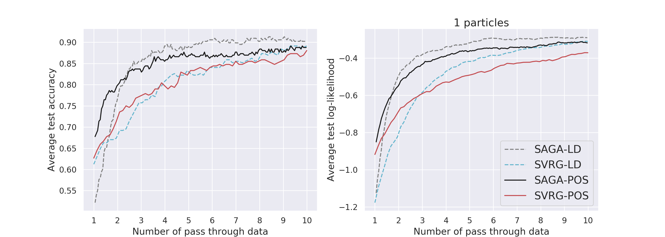
(a) 1 particle

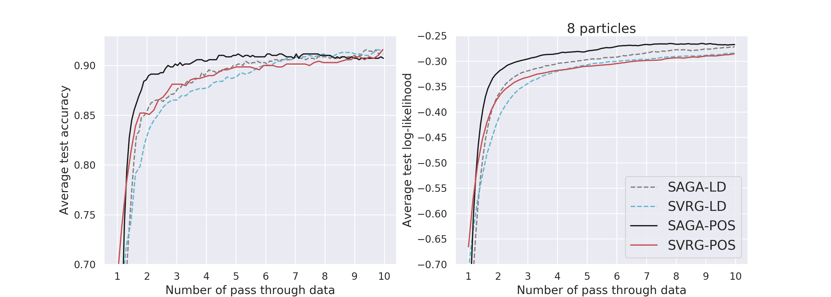
(b) 8 particles

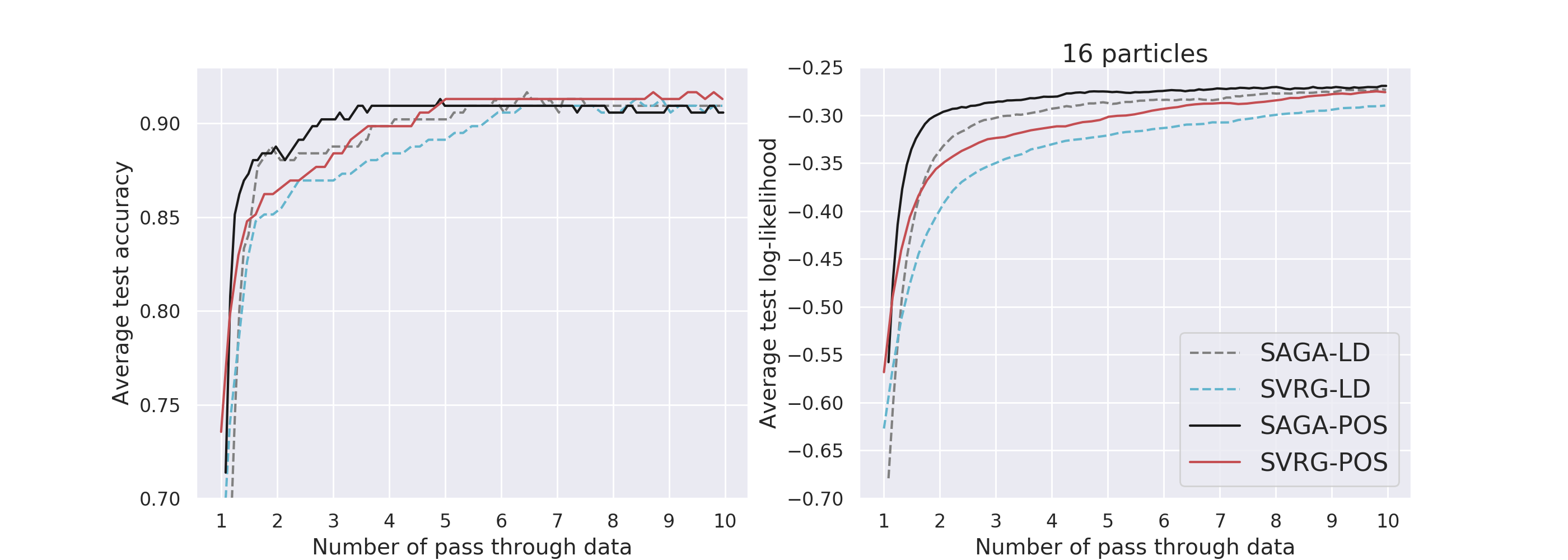
(c) 16 particles

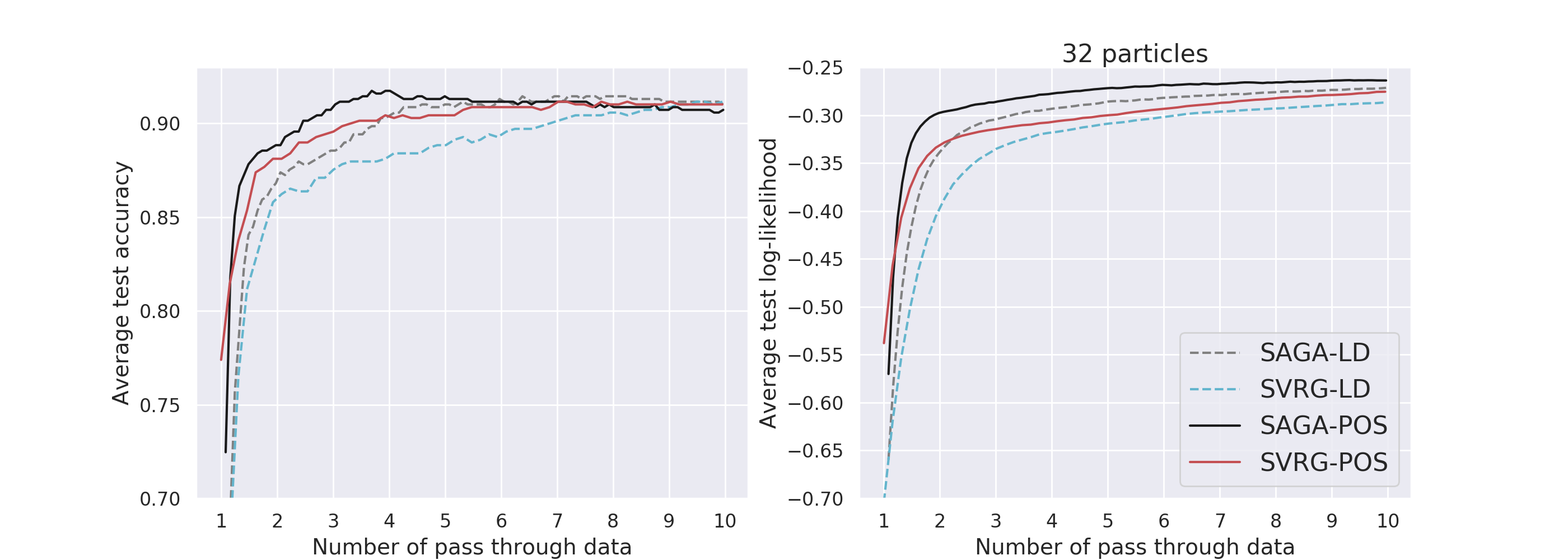
(d) 32 particles

Figure 5: Testing accuracy and log-likelihood vs the number of data pass for SPOS with varying number of particles.

References

• cBCR [16] U. Şimşekli, R. Badeau, A. T. Cemgil, and G. Richard. Stochastic Quasi-Newton Langevin Monte Carlo. In ICML, 2016.
• CFG [14] T. Chen, E. B. Fox, and C. Guestrin. Stochastic gradient Hamiltonian Monte Carlo. In ICML, 2014.
• CFM+ [18] Niladri Chatterji, Nicolas Flammarion, Yi-An Ma, Peter Bartlett, and Michael Jordan. On the theory of variance reduction for stochastic gradient monte carlo. ICML, 2018.
• CZW+ [18] C. Chen, R. Zhang, W. Wang, B. Li, and L. Chen. A unified particle-optimization framework for scalable Bayesian sampling. In UAI, 2018.
• DBLJ [14] Aaron Defazio, Francis Bach, and Simon Lacoste-Julien. Saga: A fast incremental gradient method with support for non-strongly convex composite objectives. Nips, 2014.
• DFB+ [14] N. Ding, Y. Fang, R. Babbush, C. Chen, R. D. Skeel, and H. Neven. Bayesian sampling using stochastic gradient thermostats. In NIPS, 2014.
• DK [17] Arnak S. Dalalyan and Avetik Karagulyan. User-friendly guarantees for the langevin monte carlo with inaccurate gradient. arxiv preprint arxiv:1710.00095v2, 2017.
• DM [16] Alain Durmus and Eric Moulines. High-dimensional bayesian inference via the unadjusted langevin algorithm. arXiv preprint arXiv:1605.01559, 2016.
• DRP+ [16] A. Dubey, S. J. Reddi, B. Póczos, A. J. Smola, and E. P. Xing. Variance reduction in stochastic gradient Langevin dynamics. In NIPS, 2016.
• GCH+ [15] Z. Gan, C. Chen, R. Henao, D. Carlson, and L. Carin. Scalable deep Poisson factor analysis for topic modeling. In ICML, 2015.
• JZ [13] Rie Johnson and Tong Zhang. Accelerating stochastic gradient descent using predictive variance reduction. NIPS, 2013.
• Kol [31] A. Kolmogoroff. Some studies in machine learning using the game of checkers. Mathematische Annalen, 104(1):415–458, 1931.
• LCCC [16] C. Li, C. Chen, D. Carlson, and L. Carin. Preconditioned stochastic gradient Langevin dynamics for deep neural networks. In AAAI, 2016.
• LCLC [17] B. Li, C. Chen, H. Liu, and L. Carin. On connecting stochastic gradient MCMC and differential privacy. Technical Report arXiv:1712.09097, 2017.
• LW [16] Qiang Liu and Dilin Wang. Stein variational gradient descent: A general purpose bayesian inference algorithm. In NIPS, 2016.
• LZS [16] C. Liu, J. Zhu, and Y. Song. Stochastic gradient geodesic MCMC methods. In NIPS, 2016.
• Ris [89] H. Risken. The Fokker-Planck equation. Springer-Verlag, New York, 1989.
• [18] Fei Xia Soheil Feizi, Changho Suh and David Tse. Understanding gans: the lqg setting. https://arxiv.org/abs/1710.10793.
• SKFH [16] J. T. Springenberg, A. Klein, S. Falkner, and F. Hutter. Bayesian optimization with robust Bayesian neural networks. In NIPS, 2016.
• WFS [15] Y. X. Wang, S. E. Fienberg, and A. Smola. Privacy for free: Posterior sampling and stochastic gradient Monte Carlo. In ICML, 2015.
• WT [11] M. Welling and Y. W. Teh. Bayesian learning via stochastic gradient Langevin dynamics. In ICML, 2011.
• ZXG [18] Difan Zou, Pan Xu, and Quanquan Gu. Subsampled stochastic variance-reduced gradient langevin dynamics. UAI, 2018.
• ZZC [18] J. Zhang, R. Zhang, and C. Chen. Stochastic particle-optimization sampling and the non-asymptotic convergence theory. Technical Report arXiv:1809.01293, 2018.