Quest for the Donor Star in the Magnetic Precataclysmic Variable V1082 Sgr

Abstract

We obtained high-resolution spectra and multicolor photometry of V1082 Sgr to study the donor star in this 20.8 hr orbital period binary, which is assumed to be a detached system. We measured the rotational velocity ($v\sin i=26.5\pm 2.0$ km s^-1), which, coupled with the constraints on the white dwarf mass from the X-ray spectroscopy, leads to the conclusion that the donor star barely fills 70% of its corresponding Roche lobe radius. It appears to be a slightly evolved K2-type star. This conclusion was further supported by a recently published distance to the binary system measured by the Gaia mission. At the same time, it becomes difficult to explain a very high ($>10^{-9}$ ${\rm M_{\odot}~{}yr^{-1}}$) mass transfer and mass accretion rate in a detached binary via stellar wind and magnetic coupling.

1 Introduction

The term magnetic pre-polars was coined by Schwope et al. (2009), when it was recognized that some magnetic white dwarfs (MWDs) are accreting matter from the secondary, an active late-type main-sequence star underfilling its Roche lobe. The spectra of these systems show strong cyclotron harmonics in the form of wide humps superimposed on the WD+M-dwarf stellar continuum. Accretion onto the MWD primary is of the order of $10^{-14}-10^{-13}$  ${\rm M_{\odot}~{}yr^{-1}}$, comparable to what is expected from the wind of a chromospherically active companion star (Schwope et al., 2002). Ferrario et al. (2015) listed 10 such systems, all of which contain M dwarfs as a donor star. It is natural to assume that there also should exist pre-polars with donor stars of earlier spectral types. It is not clear how justified the term pre-polars would be for wider systems with earlier-type companions. But let us assume that pre-polars are detached binaries consisting of a strongly MWD and any late-type zero-age main-sequence (or nearly so) magnetically active star, in which the magnetic fields are coupled, forcing synchronous rotation of the components and driving mass transfer. Observationally, pre-polars with earlier-type companions might manifest themselves differently than those containing an M dwarf.

Tovmassian et al. (2016, 2017) proposed two candidates for pre-polars with early-K companions. One of them is V1082 Sgr, remarkable for its cyclical accretion activity and low-luminosity episodes during which the K star is the predominant source of light. V1082 Sgr is a prominent X-ray source. Bernardini et al. (2013) studied it with several available X-ray telescopes and concluded that it is a highly variable X-ray source with a spectrum matching those of magnetic cataclysmic variables (CVs). They identify a small X-ray-emitting region where the plasma has typical temperatures achieved in a magnetically confined accretion flow. Using the model of Suleimanov et al. (2005), the mass of the magnetically accreting WD was estimated to be $M_{\mathrm{wd}}=0.64\pm 0.04$ M_⊙. From the derived WD mass and radius ($8.3\times 10^{8}$ cm), they deduced a mass accretion rate of $\dot{M}$= $2-4\times 10^{-9}$ M_⊙ yr^-1  for a distance of 730 pc and 1.15 kpc, respectively.

We conducted high-resolution spectroscopy accompanied by parallel multiband photometry to define the parameters of the donor star and the binary as a whole. This study comes on the heels of observations of the object by the Kepler K2 mission. Results of 80 days long of continuous, time-resolved photometry of the object are analyzed by Tovmassian et al. (2018, hereafter Paper I ). Relevant to this follow-up article is the detection of the orbital period in the K2 light curve. In V1082 Sgr, there are deep low states when the light curve appears to be dominated by the donor star. Paper I concludes that such a light curve cannot be produced by an ellipsoidally deformed star because it would create two dips per orbit, and hence the K star in this binary is not filling its Roche lobe. Instead, one dip per orbit has been observed, which was interpreted in Paper I as presence of a spot (cool, hot, or a combination of both) on the surface of the donor star.

In this paper, we approach the same problem from a different point of view to confirm that V1082 Sgr is indeed a detached binary. In Section 2, we describe our observations of V1082 Sgr and the corresponding data reduction. In Section 3 we present the analysis of a complex of absorption lines and the measurements of radial velocities (RVs). The deduction of rotational velocity is in Section 4 and the binary system parameters are presented in Section 5. In Section 6, we review the new information gathered from the emission-line profiles. We provide a discussion of the obtained results and their application in Section 7.

2 Observations

The high-resolution spectroscopic observations of V1082 Sgr were obtained using the echelle REOSC spectrograph (Levine & Chakarabarty, 1995) at the 2.1 m telescope of the Observatorio Astronómico Nacional at San Pedro Mártir (OAN SPM), Mexico. The echelle spectrograph provides spectra covering the $\sim$3500–7105 Å range with a spectral resolving power of R$\approx$18,000. A total of 42 echelle spectra were obtained during 11 consecutive nights in 2017 July. A Th-Ar lamp was used for wavelength calibration. The spectra were reduced using the echelle package in iraf. Standard procedures, including bias subtraction, cosmic-ray removal, and wavelength calibration were carried out using the corresponding tasks in iraf. The flux calibration is notoriously difficult with echelle spectra, which we did not attempt. We merged all orders after normalizing them to the continuum. In the overlapping regions, spectra were weighted according to their signal level, and the ends of the orders were apodized with a cosine bell to prevent discontinuities. These merged spectra were used for the spectral class and rotational velocity determination. There is a problem with the focus of the REOSC spectrograph, originally designed for photographic plates but now modified for a CCD camera that provides a larger field of view, and the focus deteriorates toward the ends of the spectral orders.

A number of K stars of different spectral and luminosity classes of known rotational velocities used routinely as standards (Fekel, 1997) were observed along the object. HD 182488 was primarily used for rotational velocity measurements, together with HD 166620 for RV measurements. Several others of earlier and later spectral types, as well as luminosity class IV, were observed and used for spectral class determination. The log of observations is given in Table 1.

Table 1: Log of spectroscopic observations obtained with the 2.1m telescope and the echelle spectrograph.

Date UT	JD	$t_{\mathrm{exp}}$	Number
yyyy mm dd	2,450,000+	(s)	of Spectra
2017 07 07	7941	1200	1
2017 07 08	7942	1200	2
2017 07 10	7944	1800	1
2017 07 11	7945	1200	2
2017 07 12	7946	1200	2
2017 07 13	7946	1200	2
2017 07 14	7948	1200	8
2017 07 15	7949	1200	7
2017 07 16	7950	1800	8
2017 07 17	7951	1800	7
2017 07 18	7952	1800	2

Multicolor photometric observations were obtained with the Reionization and Transients InfraRed (RATIR), a simultaneous six-filter imaging camera ($r,i,Z,Y,J$ and $H$ bands), mounted on a Harold L. Johnson 1.5 m telescope at OAN (Butler et al., 2012; Watson et al., 2012). It operates in robotic mode and is available in the absence of gamma ray burst alerts. We asked for sequences of multicolor exposures prior, during, and after the spectral observations. The telescope is not designed for prolonged monitoring or long exposures, and the guiding is very poor. Hence, the reduction of the data was very arduous and required one-by-one inspection of all images, a large fraction of which turned out to be worthless as a result of bad pointing or guiding. However, we could use the good data to produce decent light curves in the $V$, $J$ and $H$  bands, and get a good idea of the luminosity state of the object during spectroscopic observations. The images were processed using an automatic pipeline package for bias subtraction, flat-fielding, and cosmic-ray removal. The reduction pipeline also permits sky subtraction when necessary and astrometric alignment of images. For the latter, astrometry.net software was used.

After these preliminary steps, we measured the magnitudes of the object and of several similar and brighter comparison stars found in the field using the iraf task apphot within the daophot package. We used a circular aperture with 5$.\!\!^{\prime\prime}$5 radius for the object and comparison stars. The object magnitudes were then determined in a differential photometry with comparison stars of known magnitudes. We checked the comparison stars against each other to ensure that none of them were variable and determined errors of measurements as a standard deviation.

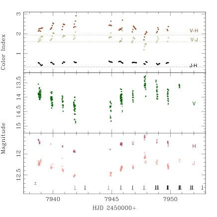
Figure 1: Light curve of V1082 Sgr in three bands during the spectroscopic observations. In the bottom panel, measurements of IR observations are plotted. Epochs of spectral exposures are marked in the bottom of the panel. In the left bottom left corner, the photometric error bar is indicated. The $V$-band light curve is presented in the middle panel, In the top panel, color indexes are presented. All photometric bands and color indexes are plotted in distinct colors and indicated on the right sides of the light curves. The horizontal dotted lines in the top panel indicate colors corresponding to a K2 main-sequence star.

3 Analysis of Absorption Lines

The spectrum of V1082 Sgr shows absorption lines from the K donor star throughout the wavelength range covered by our data set. Often the continuum is contaminated by the accretion-fueled radiation taking place in this system, as well as by emission lines of hydrogen and helium. However, as was already mentioned above, V1082 Sgr undergoes low-state episodes, when the contribution of the donor star is overwhelming. There appear to be brief intervals when the accretion stops completely, exposing pure K-type spectrum in the optical range. Tovmassian et al. (2016) demonstrated examples of such spectra and suggested a K2 spectral class. In the new, high-resolution observations, we caught the system in the deep minimum, but it was too faint to get a good signal-to-noise (S/N) ratio spectrum with the echelle spectrograph. However, for the analysis of absorption lines and their profiles, the spectra obtained in a higher-luminosity state are fine, since absorption lines are better exposed on the background of the elevated continuum. In Figure 1 the spectral exposures are marked at the bottom of the light curve obtained by RATIR in near-IR filters. The brightness of the system constantly changes with the S/N at the continuum, reaching $\sim 20$ in the single brightest spectra and about 2 in the faintest phase.

3.1 Spectral type and RVs

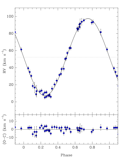
Figure 2: The RV curve of the donor star measured by cross-correlation with the synthetic spectrum. Systemic velocity is marked with a dotted line. The parameters of the average fit are presented in Table 2.

Measurements of RVs improved greatly compared to previously available data (Thorstensen et al., 2010; Tovmassian et al., 2016). We cross-correlated the ranges of spectra containing multiple strong absorption features with reference spectra of standard stars. We used spectra of HD 182488 (K0 V), HD 166620(K2 V), which were observed with the same instrumental settings together with the object, and a synthetic spectrum of $T_{\mathrm{eff}}=5000$ K taken from the bluered database (Bertone et al., 2008). We refined the orbital period by analyzing the new RV measurements in combination with the previous data (Tovmassian et al., 2016) for a longer time base. We fitted the RV curve using only data from high-resolution observations by fixing the period obtained from a larger database. The differences in the results obtained using different templates are negligible. Formal errors of measurements are smaller by a factor of $\sim 2$ in the case of the synthetic spectrum, although the residuals are similar for either case (only $\sim 10$% smaller). The RV measurements are included in electronic tables accompanying the paper.

The results of all measurements are summed up in Fig. 2 and Table 2. The parameters listed in the table are time of primary conjunction, center-of-mass velocity, velocity amplitude, orbital period, and standard deviation of residuals. The orbit was assumed to be circular.

Table 2: Parameters of the RV Curve.

$T_{\mathrm{0}}$	HJD	2,457,939.161$\pm$	0.002
$V_{\gamma}$	km s-1	51.8$\pm$	0.6
$K_{d}$	km s-1	45.3$\pm$	0.7
$P$	days	0.867525$\pm$	0.000015
$\sigma$	km s-1	2.8

Figure 3: Comparison of the spectral morphology of V1082 Sgr with reference spectra of different spectral types. HD 182488 (K0 V), HD 142980 (K1 IV), HD 115404 and HD 166620 (averaged as K2 V), and HD 219134 (K3 V) were observed along with V1082 Sgr during the same period of observations.

In order to produce a high-S/N spectrum of the donor star, we proceeded as follows. First, we corrected the Doppler displacement of each merged spectrum according to the measured RV of the absorption lines. Then, we estimated the light contribution of the donor star by comparing the spectral-line intensities with those of a standard star. More precisely, we calculated the multiplying factor minimizing the difference between the object spectrum and the scaled reference spectrum in four small selected spectral regions and then averaged the four values into a single scale factor for each spectrum. Typically, the scale factors range from 0.25 to 0.6 depending on the luminosity state of the object, as reflected in the light curve presented in Figure 1.

Then the lines of the donor star were removed from each spectrum to measure the noise and identify deviant pixels to be removed. The individual spectra corrected for RV, after being scaled and cleaned, were combined to produce an average spectrum. In this calculation, we used optimal weights that were calculated from the scale factors and the measured noise.

We compared the combined averaged spectrum with reference spectra of different spectral types. We selected from the Simbad database stars in the temperature range 4500–5500 K, with solar metallicity (0.0$\pm$0.1 dex), and surface gravity corresponding to main-sequence stars ($\log g$ = 4.3–4.6). Then, we downloaded from the ESO archive high S/N ($>200$) spectra of these objects taken with the HARPS spectrograph.

The selected stars are listed in Table 3.

Table 3: List of Stars Used to Produce Templates

star	$T_{\mathrm{eff}}$	$\log g$	Met	SpType
HD 131977	4669	4.29	-0.04	K4 V
HD 160346	4871	4.51	+0.00	K3 V
HD 23356	4924	4.55	-0.08	K2.5 V
HD 192310	5077	4.50	+0.04	K2 V
HD 22049	5090	4.55	-0.07	K2 V
HD 149661	5254	4.54	+0.03	K1 V
HD 165341	5260	4.51	+0.00	K0 V
HD 69830	5396	4.47	-0.05	G8 V
HD 152391	5467	4.49	-0.02	G8 V

Finally, we built spectral templates by combining some of these spectra and convolving them with an appropriate rotational profile (25 km s^-1) and scaled by a factor of 0.5 in order to make them consistent with that of V1082 Sgr, whose lines are reduced by the light contribution from the companion. The final templates were T4660 (HD 131977), T4900 (average of HD 160346 and HD 23356), T5080 (HD 192310, HD 22049), T5250 (HD 149661, HD 165341), and T5430 (HD 69830, HD 152391).

We looked for metallic lines that can be used for spectral-type classification in the spectral regions less contaminated by the companion. Fig. 3 shows the spectrum of V1082 Sgr in comparison with the reference spectra. Some V I-to-Fe I and Cr I-to-Fe I line ratios are sensitive to temperature. Another good indicator is the aspect of the $\lambda$4227 Ca I line. In all cases, the line ratios suggest a spectral type of K2 V (templates T4900 to T5250).

The surface of the donor is likely to have spots, similar to the chromospherically active stars (Berdyugina, 2005), so the temperature measurements vary with orbital phase (e.g. Watson et al., 2007). It is clear from the spectrum that the donor star in V1082 Sgr  is not a giant star, but whether the spectrum corresponds exactly to a normal-size main-sequence star or is slightly larger is hard to tell from the spectral features. We are inclined to identify the donor star of V1082 Sgr as K1 V-K2 V. The high-resolution spectra thus confirm the results obtained previously by Tovmassian et al. (2016), but make the classification more reliable.

4 Rotation

The Kepler K2 mission 80 days of continuous photometry shows that the orbital period is present in the light curve during the low state (Paper I). The period appears as a smooth, nearly sinusoidal, single-humped wave during a deep minimum when the optical flux is produced predominantly by the K star. The observed light curve is interpreted as an evidence that the K star is not deformed by overflowing its Roche lobe but has a spot or spots on its surface, reflecting its rotational period. Since the rotation can be safely assumed to be synchronous, the projected rotational velocity can give information about the radius of the late-type stellar companion. In a first trial, we determine $v\sin i$ using the method developed by Díaz et al. (2011), which allows us to deal with the line blending present in late-type stars. This technique reconstructs the rotational profile from the cross-correlation function of the object spectrum against a sharp-lined template and derives the rotational velocity from the first zero of the Fourier transform (FT) of the rotational profile. In these calculations, we adopted limb-darkening coefficients from Neilson & Lester (2013).

Measuring the rotational velocity is a difficult task for this object. Several factors conspire against a reliable determination. Díaz et al. (2011) mentioned that the method works satisfactorily when the rotational broadening is larger than the instrumental profile (or other broadening effects) by a factor of 2. In the present case, the rotational broadening ($v\sin i\approx 27$ km s^-1) is relatively low in comparison to the spectral resolution (the FWHM of the instrumental profile is about 18-20 km s^-1). On the other hand, the S/N ratio is modest ($\sim 20$ for individual observations, $\sim$80 for the average spectrum), which is aggravated by the dilution of the spectral lines due to the light contribution of the companion.

Finally, the useful spectral regions are rather limited, since regions contaminated by the companion emission lines must be excluded, as well as those containing the strongest lines of the late-type star itself, since such line profiles are affected by pressure broadening. Some examples of the power spectra of the line profiles are shown in Fig. 4.

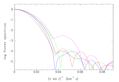
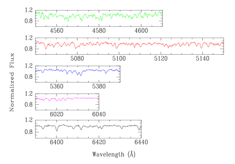
Figure 4: The FT of the autocorrelation function between the selected regions containing absorption lines and the template is presented in the top panel. The first zero of the FT corresponds to the rotational velocity (see Díaz et al. (2011) for details). The selected spectral regions are plotted in the bottom five panels. The FT power of each region is plotted with a corresponding color.

We applied the mentioned technique to a few selected regions presented in the bottom part of Figure 4 . In the best three regions, we obtained $v\sin i$ = 27.7$\pm$1.0 km s^-1, 27.6$\pm$ 2.5 km s^-1, and 26.3$\pm$1.5 km s^-1, while some other failed to define a reliable zero FT at all.

As a second strategy, we estimated $v\sin i$ by comparing the target spectrum with a template previously convolved with different rotational profiles. We used as a reference the observed spectrum of HD 182488, which was convolved with rotational profiles between 22 and 32 km s^-1. The comparison was done by cross-correlating each spectrum against the original reference spectrum and measuring the FWHM of the central peak of the cross-correlation function. The rotation of reference star is below the spectral resolution and has a negligible contribution to the peak FWHM.

The main advantage of this method with respect to the former is that the contribution of the instrumental profile is less critical. Particularly, the mentioned problem of deficient focus over the CCD (variable instrumental profile along the spectrum) is largely mitigated by the fact that both object and reference spectra are taken under the same conditions and, therefore, are affected in the same way. Hence, we considered this strategy more reliable and applied it to 10 spectral regions ranging from 4250 to 6450Å. We used as a template the spectrum of HD 182448 (a sharp-lined K0V star) taken with the same instrument. It is probably slightly hotter than the object, and their chemical abundances do not match exactly. However, the very low $v\sin i=0.6$ km s^-1  rotational velocity of the template and variety of lines used for measurements make it suitable for the task.

We also considered the effect of velocity smearing on our measurements as an outcome of relatively long exposure times (1200 s) used in observations. We convolved synthetic spectrum representing the intrinsic stellar spectrum (with $v\sin i=26.5$ km s^-1) with boxy kernels of widths equal to the RV variation during the exposure time. We calculated the mean spectrum and measured the rotation with the same procedure as described in this section. The results showed that our measurement of $v\sin i$ would be about 0.3 km s^-1  above the true value, that is, well below the uncertainties cited below.

The obtained values of $v\sin i$ average at $25.3\pm 2.4$ km s^-1  within small error spread. However, for three regions below $\lambda 4900\AA$, the values are slightly smaller and show tendency to decrease toward shorter wavelengths. The contribution of the donor star at shorter wavelengths drops rapidly when the object is not in deep minima, hence the measurements at the blue end of the spectra are less reliable. Excluding these three values, we obtain $v\sin i=26.5\pm 1.4$ km s^-1 of a very stable subsample.

Considering the possible differences in the instrumental profile between the observations of the object and reference star, we adopted a value of 26.5$\pm 2.0$ kms for the projected rotational velocity of the donor companion. Either method has its uncertainties and limitations, and probably the statistically derived error bars are underestimated, but matching results of independent measurements assure that the result is realistic.

5 Stellar Parameters

If we assume that the rotation of the K-type star (marked with subindex ”d” for ”donor”) is synchronized with the orbital motion, the relative radius of this star can be written as

$$\frac{R_{\mathrm{d}}}{a}=\frac{q}{(1+q)}\cdot\frac{v_{\mathrm{d}}\sin i}{K_{\mathrm{d}}},$$ (1)

where $q=M_{\mathrm{wd}}/M_{\mathrm{d}}$ is the mass ratio. On the other hand, according to Eggleton (1983), the effective radius of the Roche lobe in units of the orbital semiaxis can be calculated through the expression

$$\frac{R_{\mathrm{L}}}{a}=\frac{0.49}{0.6+q^{2/3}\cdot\ln\left(1+q^{-1/3}\right)},$$ (2)

which is better that 1% for any value of the mass ratio.

From these two equations, we obtain the ratio between the stellar radius and the critical radius:

$$\frac{R_{\mathrm{d}}}{R_{\mathrm{L}}}=\left(\frac{v_{\mathrm{d}}\sin i}{K_{\mathrm{d}}}\right)\cdot\frac{\left[0.6+q^{2/3}\ln\left(1+q^{-1/3}\right)\right]}{0.49\,(1+q^{-1})}$$ (3)

The first factor is known from the spectroscopy: $(v_{\mathrm{d}}\sin i/K_{\mathrm{d}})=0.586\pm 0.045$. Then, the constraint imposed by the Roche lobe on the donor star volume ($R_{\mathrm{d}}\leq R_{\mathrm{L}}$), provides an upper limit for the mass ratio: $q\leq 1.42\pm 0.2$.

Fortunately, we have strong constraints on the mass of the compact companion from the X-ray spectroscopy. Bernardini et al. (2013) derived a WD mass of $M_{\mathrm{wd}}=0.64\pm 0.04$ M_⊙ by modeling the spectrum obtained by XMM-Newton EPIC and Swift BAT.

For a comprehensive analysis of the possible configurations, we calculated $a$, $M_{\mathrm{d}}$, $R_{\mathrm{d}}$ and $R_{\mathrm{L}}$ for different possible values of $q$. More precisely, from $M_{\mathrm{wd}}$ and $q$, we calculated the mass of the donor star $M_{\mathrm{d}}$ and the total mass, and from the Kepler equation, we calculated the orbital semiaxis. Then the radii of the donor $R_{\mathrm{d}}$ and that of its Roche lobe $R_{\mathrm{L}}$ were calculated from equations 1 and 2.

The results are shown in Fig. 5. The radius of the donor star $R_{\mathrm{d}}$ is plotted as a function of $M_{\mathrm{d}}$ with a blue line; blue dashed lines mark the uncertainty interval of the radius due to the error in $v\sin i$. The radius of the Roche lobe corresponding to the donor star is plotted with a violet line.

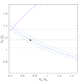
Figure 5: Mass-radius diagram for the donor star in V1082 Sgr. The black dot represents our best solution. The blue line (with limits marked as dashed lines) is the solution from the dynamical constraints. The violet line is the Roche lobe size. The green line is the radius of the donor star determined by the distance modulus The limits mark an error strip related to the temperature ambiguity (dash-dotted lines). See text for the explanation.

The adopted solution is marked in Fig. 5 by a black dot. The full solution of the binary system parameters are summarized in Table 4. The consigned uncertainties have been calculated taking into account the observational errors in $P_{\mathrm{orb}}$, $v_{\mathrm{d}}\sin i$, $M_{\mathrm{wd}}$, and $K_{\mathrm{d}}$, and the error of $M_{\mathrm{d}}$ which has been estimated from the spectral type (see Fig. 5).

Table 4: Deduced absolute parameters of V1082 Sgr.

Parameter	Units	Value
Md	M⊙	0.73$\pm$	0.04
Mwd	M⊙	0.64$\pm$	0.04
$i$	$\deg$	23.3$\pm$	1.3
$q$		0.88$\pm$	0.09
$a$	R⊙	4.25$\pm$	0.07
Rd	R⊙	1.16$\pm$	0.11
RL	R⊙	1.66$\pm$	0.05

Thus, the donor fills only a fraction of its Roche lobe (about one-third of the corresponding volume), although it is significantly ($\sim$70%) larger than a nonevolved main-sequence star of the same mass. In fact, the evolution of stars of such masses is so slow that this mass-radius relation can be explained only as the result of a nonstandard evolution.

5.1 Stellar parameters: Gaia Distance

While this paper was in the final stages of preparation, the second Gaia data release (Gaia DR2; Gaia Collaboration et al., 2016), which provides precise parallaxes for an unprecedented number of sources, became available. According to Gaia DR2, the distance to V1082 Sgr is $669\pm 13$ pc. This allows us to impose direct and stringent limits on the size of the donor star. Using the faintest visual magnitude V=14.8, repeatedly recorded during deep minima in over 1500 days; interstellar reddening of E(B-V)=0.15 (Schlegel et al., 1998), and T${}_{\mathrm{eff}}=4930$ K, a temperature corresponding to a K2-type star we obtain R${}_{\mathrm{d}}=1.165$ R_⊙. If we take into account the uncertainty in temperature of up to $350$ K, which is the largest factor affecting the luminosity, we obtain a range of values of the donor star R${}_{\mathrm{d}}=1.03-1.34$ R_⊙, independent of the mass of the binary components. This range of values is marked in Fig. 5 as a horizontal strip within dash-dotteded green lines, with the central value exactly corresponding to what we deduced before the distance was known.

6 Analysis of Emission Lines

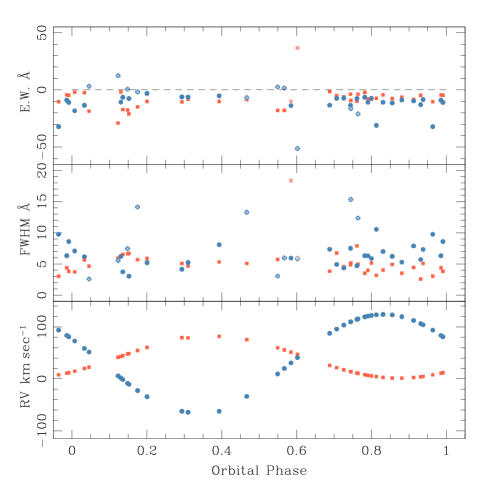
Figure 6: Parameters of two components of emissionline He II marked by red squares and blue circles. The RVs are presented in the bottom panel, the FWHMs in the middle panel, and EWs in the top panel. Three iterations of the deblending procedure were made to find solutions that correspond to two components with strictly periodical RVs. The central wavelengths, FWHMs, and core intensities of these components were used to produce the profiles shown in Figure 7. The horizontal dotted line in the top panel corresponds to zero. Points above that line are invalid and marked with crosses. Also marked with crosses are the points with extremely broad components, as can be seen in the middle panel.

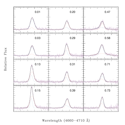
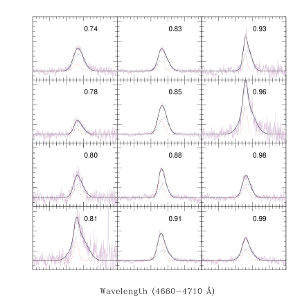
Figure 7: Examples of disentangling emission-line He II into two components, plotted by red and blue dotted lines. Black curves correspond to the sum of the two components, while the observed spectra are plotted in light violet. The vertical axes are in normalized counts, with a continuum corresponding to one unit. The numbers in each box indicate the orbital phase at which that spectrum was taken.

From the previous lower-resolution spectroscopy, it was known that the emission lines are single-peaked and fairly symmetric (Tovmassian et al., 2016). However, measuring emission lines in the low-resolution spectra as a single line has been producing RVs of low amplitude and a huge scatter of points that was not the result of measurement errors. The amplitudes and phases of different emission lines were vastly different too, indicating that the situation was not assessed correctly.

At higher resolution, the profiles of lines appear to be not as symmetric as was thought, and we made an attempt to discern them into two components. The attempt was particularly successful in the case of the He II $\lambda 4685.75\,\AA$ line, which is somewhat sharper than the Balmer lines. We first used the deblending option of the IRAF splot procedure to fit each profile with two Gaussians. For each spectrum, we obtained a pair of RV values corresponding to two components. By eye inspection, we selected one component per spectrum that appeared to belong to a sinusoidal pattern in the RV-vs-orbital phase diagram. It was not possible to identify the right component in every spectrum, but in more than half of the cases, the selected points formed a clear pattern that could be fit with a sine curve with the orbital period. We calculated the central wavelength of that component for each spectrum and iterated the deblending procedure for all spectra, but this time keeping one component’s central wavelength fixed and another as free. We also set the FWHMs of both Gaussians as free parameters. The measurements of the second component formed a periodic pattern too, reasonably well fitted with another sinusoid. Finally, we did a third iteration of deblending by fixing the central wavelengths of both components according to the calculated sinusoids and leaving the FWHM and intensities variable. We obtained excellent fits to the line profiles in most of the cases. In only in 10 spectra out of 38, the program could not find two emission components with reasonable parameters.

In order to separate emission lines into two components, we assumed that they move sinusoidally. We defined the most readily identifiable component and then refined the parameters of the other one. Of course, this is a very idealistic approach; the reality has to be much more complicated, because the gas streams producing emission lines have intrinsic velocities and directions not coinciding with the orbital motion.

The RV measurements of these two components are plotted against the orbital phases in the bottom panel of Figure 6. The points correspond to the calculated central wavelengths that were fixed in the last deblending attempt; hence, they form a perfect sinusoids. The orbital phases are calculated according to the ephemeris determined by absorption spectra. In the middle panel of Figure 6 the FWHMs of both components are plotted. Most are very consistent with the general trend. Some strongly deviate, indicating problems usually related to the phases in which both components crisscross and become indistinguishable. In such a case, the program tends to pick a broad second component extending to the noise in the continuum or use an absorption component. Such cases appear as points above the dotted line corresponding to zero in the top panel of Figure 6, which depicts the equivalent weights (EWs) of the components. Those points in the plot are marked by red crosses. Among them are also some points that have large FWHM, inconsistent with the average.

In Figure 7 examples of line profile fits are presented. We omitted orbital phases (marked by numbers in each panel) in which the lines were not split into two components correctly, with one component being in absorption. In the other case, one of the components is getting too wide, like in phases $\phi=0.47$ and 0.58, as a consequence of both of them getting too close and difficulty in separating them. Although the procedure of selecting components and fixing central wavelengths is somewhat arbitrary, the final result is encouraging. Both components show larger RV amplitudes than the entire line when measured with a single Gaussian.

The component marked in red color in Figures 6 and 7 maintains rather stable FWHM throughout all orbital phases. Neither component appears to vary strictly in antiphase from the absorption line. Neither it is expected to be related to the stellar elements of the binary. Invalid points constitute a quarter of all measurements and do not influence the general interpretation.

We assume that the emission lines are produced by the ionized gas between the stellar components. The lines practically disappear when the accretion is halted and the system is in a deep minimum. Hence, we do not have RV measurements for the first 3 nights, when the lines were faint or absent. After the accretion is reestablished, the disentangled components of the He II line act similar to polars, showing phase shifts and high velocities related to the stream intrinsic velocity rather than the orbital velocity. The brightness of the object varies significantly in very short timescales (Paper I), and the intensity of the lines changes accordingly.

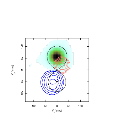
Figure 8: Doppler maps of an absorption line and two components of He II emission. All lines are artificially made with RVs of measured lines and average FWHM and intensities. The image map corresponds to the donor star while the higher-velocity (blue) and the lower-velocity (red) components are presented in the form of isochrones. The Roche lobes and stellar position are marked according to Table 4.

In an attempt to better understand the components of the emission lines, we used Doppler tomography. The system has a rather small inclination for sensible tomograms to be made. Observed lines or their components of variable intensity and width make the reading of tomograms impossible. Hence, we made artificial lines of fixed FWHM and intensity with RVs and phases of the real components. The FWHM was fixed at 5 and 7.5 Å  for the lower- and higher-velocity components, respectively, according to their averages. We also added an artificial narrow (FWHM$=0.7$ Å  absorption line emanating from the secondary to make the Doppler map more illustrative. Doppler maps of these three lines are presented in Figure 8. The inclination angle and masses derived from observations and listed in Table 4 were used to plot the Roche lobes and star locations on the Doppler map.

The intensity of the lines is not irrelevant, but since there is no a well-established pattern of line intensity and FWHM change with the phase, we kept them constant in all cases. The artificial spectra were distributed unevenly by phases, according to observations. Hence, the spots on the map are not ideally round. One has to bear in mind that this image is simplistic and may not reflect all the complexity of ionized gas distribution in the binary.

The Doppler map illustrates where in the velocity coordinates the lines originate. The high-velocity emission component is concentrated in the third quadrant. It may correspond to the accretion curtain component observed in polars as described by Heerlein et al. (1999, see Figure 5). The ballistic component is obviously absent; instead, we have a lower-velocity component in the first quadrant, practically in between the stars. This component may originate in the gas flowing along the coupled magnetic lines (magnetic bottleneck).

Parsons et al. (2013) detected similar line components (corresponding to the magnetic bottleneck) in a detached binary, but with an M-type donor star. The RV and phasing of the fainter of two components of H_α that they observed indicate that it comes from gas located in between the stars.

To pinpoint the donor star on the tomogram, we use the simulated absorption line. The absorption line produces a spot in the tomogram corresponding to the center of mass of the K star.

7 Discussion and Conclusions

We conducted high-resolution spectroscopy of V1082 Sgr, proposed to be one of two possible candidates for a pre-polar with an early-K-type donor star (Tovmassian et al., 2017). This spectroscopic study was accompanied by a prior continuous, 80 day photometry of the object by the Kepler K2 mission. The results of the photometry are reported in a separate publication (Paper I). For a wholeness of argument, we must repeat the main conclusion of Paper I: the orbital modulation detected in the light curve of V1082 Sgr persists during the deep minima, when the donor star is the predominant source of light. It is argued that the variability is caused by spots on the surface (either hot, cold, or a combination of both). No double hump is detected in the light curve. Hence, it is concluded that the donor star is not ellipsoidal and that it rotates with the orbital period. By measuring the rotational velocity of the donor star, we can go a step further and estimate other important parameters of the binary system.

These parameters are listed in Table 4. According to them, the donor star occupies about 70% of its corresponding Roche lobe radius, nevertheless exceeding the main-sequence star size of similar temperature. This means that the donor star has probably departed from the zero-age main sequence.

These estimates and conclusions are based on the assumption that the WD in this detached binary accretes as a polar and has a rather average mass for a WD according to the spectrum of the X-ray emission.

While there is no direct evidence of an MWD, it is obvious that the donor star is magnetically active and has large spot(s) on its surface. A possible explanation of the mass transfer and accretion on the WD is the magnetic coupling, capture of the stellar wind from the donor star, and channeling (siphoning) of the matter onto the magnetic pole of the WD. Doppler maps of the He II line, which consists of two components, testify that the ionized gas is not emitting from areas and spots associated with the accretion disk or streams proper to ordinary polars. This has been observed already in compact binaries comprised of an MWD and an M-type star (Parsons et al., 2013) for which the pre-polar phenomenon is well established. However, significant differences may appear if the binary contains an earlier spectral-type donor star.

These differences are related to the fact that a more massive donor star has a large convective envelope with an intense chromospheric activity, has a higher-rate stellar wind, and is prone to evolution in a Hubble time, unlike M-dwarf companions. The separation of the binary is also larger, and the mass ratio is reversed (as compared to pre-polars with M components or CVs), making the Roche lobe of the donor star much bigger than the size of a main-sequence star and hence providing a long time for evolution until the binary becomes semidetached.

There is a lack of knowledge regarding stellar winds in general and their dependence on rotational velocity due to the large spread in rotation rates of isolated stars at young ages. However, the latest models predict that the mass-loss rate due to the stellar wind depends moderately on the mass of low-mass stars, and more significantly on the rotational velocity (Johnstone et al., 2015, and references therein). Most of the observational studies of mass loss by stars of solar mass and below presume that the rotation slows down because of magnetic braking and the diminishing stellar wind. Wood et al. (2002) estimated that at younger ages, the solar wind may have been as much as $10^{3}$ times stronger. This enables a steep increase of the mass-loss rate estimate from the fast-rotating donor star in V1082 Sgr  compared to identical single stars. Chromospheric activity and a larger surface area can further fuel the mass loss. The mass-loss rate appears to depend on the X-ray surface flux as a power law (Wood et al., 2002).

The X-ray flux from V1082 Sgr in the minimum is probably due to the donor star, while the accretion on the WD is halted. The flux matches an upper limit observed from similar magnetically active stars. Thus, all prerequisites exist to expect a mass accretion rate a few orders higher than that in pre-polars with an M-star companion.

Another thorny issue is how a mass loss from the donor star converts into the mass accretion on the WD. Cohen et al. (2012) demonstrated that matter lost through the stellar wind will not always find its way to the WD. There are configurations in which all the wind can effectively siphon to the MWD. Curiously, such configurations require antialigned and require rather modest magnetic fields. However, it is still incomprehensible how the accretion rate reaches an estimated $2\times 10^{-9}$ M_⊙  yr^-1 (Bernardini et al., 2013) in V1082 Sgr. With the Gaia distance, this rate is 1.3 times less, but is still of the same order.

The accretion is not continuous, however. It is regularly interrupted by deep minima states where there is no evidence of accretion at all. We speculate that the cessation of accretion is related to the broken magnetic coupling. The deep minima last only a few orbital periods, then the accretion is restored.

Such a high accretion rate exceeding that of an ordinary CVs is unusual and raises questions about how it will affect the evolution of the binary system. The excess nitrogen abundance probably indicates that V1082 Sgr has formed from massive progenitors and underwent an episode of thermal time-scale mass transfer, as was pointed out by Bernardini et al. (2013, and references therein).

We found independent observational evidence suggesting that V1082 Sgr is a detached binary containing a slightly evolved early-K star. If this proposition is correct, we see no alternative to the magnetic coupling as the means of transferring matter and angular momentum from the donor to an MWD. This object corroborates the existence of pre-polars with earlier spectral-type donor stars. It offers an explanation as to why magnetic systems are not found in the search for detached WD+FGK detached binaries (Parsons et al., 2016; Rebassa-Mansergas et al., 2017). Yet the object presents certain challenges. It is necessary to estimate the magnetic field strength of the WD and its temperature and mass directly by UV observations. Furthermore, it is necessary to calculate possible evolution scenarios in conditions of a high mass transfer rate while the system is still detached and where it will evolve.

References

- Berdyugina (2005) Berdyugina, S. V. 2005, Living Reviews in Solar Physics, 2, 8
- Bernardini et al. (2013) Bernardini, F., de Martino, D., Mukai, K., et al. 2013, MNRAS, 435, 2822
- Bertone et al. (2008) Bertone, E., Buzzoni, A., Chávez, M., & Rodríguez-Merino, L. H. 2008, A&A, 485, 823
- Butler et al. (2012) Butler, N., Klein, C., Fox, O., et al. 2012, in Proc. SPIE, Vol. 8446, Ground-based and Airborne Instrumentation for Astronomy IV, 844610
- Cohen et al. (2012) Cohen, O., Drake, J. J., & Kashyap, V. L. 2012, ApJ, 746, L3
- Díaz et al. (2011) Díaz, C. G., González, J. F., Levato, H., & Grosso, M. 2011, A&A, 531, A143
- Eggleton (1983) Eggleton, P. P. 1983, ApJ, 268, 368
- Fekel (1997) Fekel, F. C. 1997, PASP, 109, 514
- Ferrario et al. (2015) Ferrario, L., de Martino, D., & Gänsicke, B. T. 2015, Space Sci. Rev., 191, 111
- Gaia Collaboration et al. (2016) Gaia Collaboration, Prusti, T., de Bruijne, J. H. J., et al. 2016, A&A, 595, A1
- Heerlein et al. (1999) Heerlein, C., Horne, K., & Schwope, A. D. 1999, MNRAS, 304, 145
- Johnstone et al. (2015) Johnstone, C. P., Güdel, M., Lüftinger, T., Toth, G., & Brott, I. 2015, A&A, 577, A27
- Levine & Chakarabarty (1995) Levine, S., & Chakarabarty, D. 1995, IA-UNAM Technical Report MU-94-04
- Neilson & Lester (2013) Neilson, H. R., & Lester, J. B. 2013, A&A, 556, A86
- Parsons et al. (2013) Parsons, S. G., Marsh, T. R., Gänsicke, B. T., et al. 2013, MNRAS, 436, 241
- Parsons et al. (2016) Parsons, S. G., Rebassa-Mansergas, A., Schreiber, M. R., et al. 2016, MNRAS, 463, 2125
- Rebassa-Mansergas et al. (2017) Rebassa-Mansergas, A., Ren, J. J., Irawati, P., et al. 2017, MNRAS, 472, 4193
- Schlegel et al. (1998) Schlegel, D. J., Finkbeiner, D. P., & Davis, M. 1998, ApJ, 500, 525
- Schwope et al. (2002) Schwope, A. D., Brunner, H., Hambaryan, V., & Schwarz, R. 2002, in Astronomical Society of the Pacific Conference Series, Vol. 261, The Physics of Cataclysmic Variables and Related Objects, ed. B. T. Gänsicke, K. Beuermann, & K. Reinsch, 102
- Schwope et al. (2009) Schwope, A. D., Nebot Gomez-Moran, A., Schreiber, M. R., & Gänsicke, B. T. 2009, A&A, 500, 867
- Suleimanov et al. (2005) Suleimanov, V., Revnivtsev, M., & Ritter, H. 2005, A&A, 435, 191
- Thorstensen et al. (2010) Thorstensen, J. R., Peters, C. S., & Skinner, J. N. 2010, PASP, 122, 1285
- Tovmassian et al. (2017) Tovmassian, G., Gonzalez-Buitrago, D., & Zharikov, S. 2017, in Astronomical Society of the Pacific Conference Series, Vol. 509, 20th European White Dwarf Workshop, ed. P.-E. Tremblay, B. Gaensicke, & T. Marsh, 489
- Tovmassian et al. (2018) Tovmassian, G., Szkody, P., Yarza, R., & Kennedy, M. 2018, ApJ, 863, 47
- Tovmassian et al. (2016) Tovmassian, G., González–Buitrago, D., Zharikov, S., et al. 2016, ApJ, 819, 75
- Watson et al. (2012) Watson, A. M., Richer, M. G., Bloom, J. S., et al. 2012, in Proc. SPIE, Vol. 8444, Ground-based and Airborne Telescopes IV, 84445L
- Watson et al. (2007) Watson, C. A., Steeghs, D., Dhillon, V. S., & Shahbaz, T. 2007, Astronomische Nachrichten, 328, 813
- Wood et al. (2002) Wood, B. E., Müller, H.-R., Zank, G. P., & Linsky, J. L. 2002, ApJ, 574, 412