Multiparameter quantum metrology with postselection measurements

Abstract

We analyze simultaneous quantum estimations of multiple parameters with postselection measurements in terms of a tradeoff relation. The system, or a sensor, is characterized by a set of parameters, interacts with a measurement apparatus (MA), and then is postselected onto a set of orthonormal final states. Measurements of the MA yield an estimation of the parameters. We first derive classical and quantum Cramér-Rao lower bounds and then discuss their archivable condition and the tradeoffs in the postselection measurements in general, including the case when a sensor is in mixed state. Its whole information can, in principle, be obtained via the MA which is not possible without postselection. We, then, apply the framework to simultaneous measurements of phase and its fluctuation as an example.

I Introduction

Quantum metrology is a promising technology. It is applicable for a wide range of fields, such as quantum sensing Degen89 ; Pezze90 , quantum imaging Preza16 , and detecting gravitational waves Aasi7 ; Branford121 ; Qui96 ; Miao9 . The estimation of a single parameter has already been established Pezze102 ; Huelga79 ; Wineland46 ; Wineland50 ; Giovannetti306 ; Giovannetti96 ; Jones324 ; Simmons82 ; Zaiser7 ; Matsuzaki120 . Therein, several studies demonstrated the quantum-enhanced metrology by using entangled resources Pezze102 ; Huelga79 ; Wineland46 ; Wineland50 ; Giovannetti306 ; Giovannetti96 ; Jones324 ; Simmons82 , quantum memory Zaiser7 , or teleportation Matsuzaki120 . Note, however, that it is often demanded simultaneous multiparameter estimations in many practical applications. For example, estimation of phases are always affected by environmental noise and thus, a simultaneous measurement of the phase and its fluctuation is necessary. Such joint estimations have been discussed recently Vidrighin5 ; Altorio92 ; Szczykulska2 ; Sergey2013 ; Crowley89 ; Roccia2018 ; Pinel88 ; Gagatsos96 . Also, the current generation of laser-interferometric gravitational wave detectors, such as LIGO Abadie7 ; Aasi7 , are inevitably affected by squeezing noises and optical loss, therefore the improvement of the detectors can be expected when the phase and its loss are measured simultaneously. Furthermore, various practical applications have been discussed, including damping and temperature Monras83 , two-phase spin rotation Vaneph1 , waveform Berry5 , operators Fujiwara65 ; Ballester69 , phase-space displacements Genoni87 ; Steinlechner7 . The estimations of multiple phases Humphreys111 ; Liu2 and parameters in multidimensional fields Baumgratz116 ; Ho2020 have been discussed, too.

Typically, a sensor characterized by multiple parameters will be measured by a set of POVMs to estimate the parameters. We term it as “direct sensing” because no ancillary systems are required. The limit of the estimation precision is imposed by quantum mechanics and bounded by a so-called quantum Cramér-Rao bound (QCRB) Holevo2011 ; Paris7 . For a single-parameter estimation, the QCRB can be achieved by projecting the states of a sensor on the basis determined by eigenvectors of its symmetric logarithmic derivative (SLD) operator Vidrighin5 ; Crowley89 ; Dominik97 . However, for a multiparameter estimation, SLD operators of different parameters may not commute and thus the basis determined by them may not be orthonormal. Such a case leads to a tradeoff in the estimation of different parameters Crowley89 ; Szczykulska2 ; Vidrighin5 ; Altorio92 . This tradeoff is a kind of “competition” among them Szczykulska1 . Although several theoretical and numerical studies of the optimal POVMs that saturate the QCRB as well as the tradeoff relations have been reported Szczykulska2 ; Yang2018 ; Pezze119 , achieving the QCRB is still a challenging task in the multiparameter estimations. Alternatively, one can consider a so-called Holevo Cramér-Rao bound, which is asymptotically achievable and can reach twice times larger than the QCRB. See Rafal2020 and references therein.

In contrast to the “direct sensing,” an “indirect one” with postselection is also possible for parameter estimations, hereafter referred to as a postselection measurement. The sensor interacts with an ancillary system, referred to as a measurement apparatus (MA). After the interaction, the sensor will be postselected while the final MA state will be measured to provide the estimation. Postselection measurements have been used to estimate single parameters Knee87 ; Tanaka88 ; Knee4 ; Combes89 ; Ferrie112 ; Zhang114 ; Chen121 ; Pang113 ; Pang92 ; Alves91 ; Alves95 ; Dressel88 ; Lyons114 ; Wang117 ; Pang115 ; Jordan4 ; Jordan2 ; Pang94 ; Harris118 ; Viza92 ; Sinclair96 ; Ho383 and various methods have been proposed, including the optimal choices of the system and MA states Alves91 ; Alves95 , entangled sensors Pang113 ; Pang92 , photon recycling Dressel88 ; Lyons114 ; Wang117 , non-classical MA Pang115 to improve the precision. There are, however, ongoing debates over the merit of postselection measurements if it defeats the ultimate-limit precision or not. Most studies point out that postselection measurements cannot provide any advantages for the estimations Knee87 ; Tanaka88 ; Knee4 ; Combes89 ; Ferrie112 ; Zhang114 ; Chen121 ; Pang113 ; Pang92 . It is true because the postselection measurements do not generate “information”. Thus, they alone cannot beat it, even though all the data (from the success and failure postselections) are taken into account Knee87 ; Combes89 ; Ferrie112 ; Zhang114 ; Chen121 . For example, Knee et al. Knee87 ; Knee4 , Tanaka and Yamamoto Tanaka88 claimed that quantum Fisher information obtained from the success postselection alone could not overcome the QCRB. However, there are still some benefits of using postselection measurements. There are reports on achieving the Heisenberg scaling of the single parameter estimation using postselection measurements Zhang114 ; Chen121 ; Pang113 ; Pang92 ; Jordan4 ; Jordan2 . There may also be some advantages in suppressing certain types of technical noise Jordan4 ; Pang92 ; Pang115 ; Harris118 , systematic errors Pang94 . Especially, Jordan et al. claimed that for some special technical noise, indirect sensing gives higher Fisher information than a direct one Jordan4 , which was verified experimentally Viza92 . The same advantage has been found when the correlation between success and failed postselections were taken into account Sinclair96 .

Recently, multiparameter estimations using postselection measurements have been attracting a lot of attention Vella122 ; Xia13 ; Jan116 . However, the role of postselection measurements on the saturation of simultaneous multiparameter estimation has not been fully discussed yet.

In this work, we discuss the multiparameter estimations under postselection measurements. We are interested in the general case when the sensor can be in mixed state. We take into account all the orthonormal postselected states, (both the success and failed postselections.) Our work is significantly different from Tanaka and Yamamoto’s work Tanaka88 , in which only a single parameter estimation in a success mode is considered. We compare the total quantum Fisher information matrix (QFIM) obtained from all the postselection measurements (named as $\bm{Q}$) and the general QFIM determined by the sensor state only ($\bm{H}$): $\bm{H}$ corresponds to the maximum information that the sensor has. Of course, the postselection measurements cannot allow us to obtain more information from the sensor than what it has. However, as we show that the whole information in the sensor can be obtained via $\bm{Q}$ even if it is in mixed state while it cannot be done with direct measurements: We found that $\bm{Q}$ can reach $\bm{H}$. We illustrate this framework in the estimation of phase and its fluctuation since these topics have been attracting a lot of attention recently Vidrighin5 ; Altorio92 ; Szczykulska2 ; Sergey2013 ; Genoni106 .

This paper is organized as follows: Section II introduces a measurement framework with postselection, and we formulate the Cramér-Rao bounds, the condition for achieving these, and tradeoff relations. The application of our framework for measuring a phase and its fluctuation is presented in Sec. III. We summarize the results and point out the benefit of measurements with postselections in Sec. IV. Appendixes provide supporting material.

II Estimation process with postselection

A postselection measurement of a quantum system (called a sensor in this work) is as follows. It interacts with a so-called pointer which we call as a measurement apparatus (MA) in this work. After the interaction, it is postselected on a final state. Measuring the MA state reveals its information with the results of postselection.

II.1 Measurement process

We consider a quantum channel $\Lambda_{\bm{\phi}}$ that is characterized by a set of $d$ parameters ($\bm{\phi}=\{\phi_{1},\phi_{2},...,\phi_{d}\}$) to be estimated. We perform the following process. (i) A state $\rho_{\rm s,i}$ of the sensor is prepared. (ii) It evolves to $\rho^{\prime}_{\rm s,i}=\Lambda_{\bm{\phi}}(\rho_{\rm s,i})$ after passing through the quantum channel $\Lambda_{\bm{\phi}}$, which now contains the information of ${\bm{\phi}}$. (iii) The sensor and MA interact with each other and become a joint state

$$\rho_{\rm sm} =\hat{U}_{\rm sm}\bigl{(}\rho^{\prime}_{\rm s,i}\otimes|\xi\rangle\langle\xi|\bigr{)}\hat{U}_{\rm sm}^{\dagger},$$ (1)

where $|\xi\rangle$ is an initial MA state and

$$\hat{U}_{\rm sm} ={\rm exp}(-ig\hat{A}_{\rm s}\otimes\hat{M}_{\rm m}),$$ (2)

is the unitary evolution caused by the sensor-MA interaction. $g$ is the interaction strength and can be controlled. $\hat{A}_{\rm s}$ and $\hat{M}_{\rm m}$ are operators on the sensor and the MA, respectively. The role of the interaction is to share the information of $\bm{\phi}$ in the sensor with the MA. (iv) The sensor is postselected onto a final state $\rho_{\rm s,f}^{(\jmath)}=|\psi_{\rm s,f}^{(\jmath)}\rangle\langle\psi_{\rm s,f}^{(\jmath)}|$. Here, we consider a set of orthonormal postselected states with $\jmath=1,2,\dots$.

The probability of postselection into $\jmath$ is

$$w^{(\jmath)} ={{\rm Tr}[(\rho_{\rm s,f}^{(\jmath)}\otimes I_{\rm m})\rho_{\rm sm}]},$$ (3)

where $I_{\rm m}$ is the identity matrix in the MA space. When all orthonormal postselected states are taking into account, we have $\sum_{\jmath}w^{(\jmath)}=1$. The MA state after the postselection reads

$$\rho^{(\jmath)}_{\rm m}=\dfrac{{\rm Tr}_{\rm s}[(\rho_{\rm s,f}^{(\jmath)}\otimes I_{\rm m})\rho_{\rm sm}]}{w^{(\jmath)}},$$ (4)

where ${\rm Tr}_{\rm s}[*]$ is a partial trace w. r. t. the sensor. $\sum_{\jmath}\rho^{(\jmath)}_{\rm s,f}=I_{\rm s}$ by definition of the probability, where $I_{\rm s}$ is the identity matrix in the sensor space. Assume that we employ a POVM $\hat{\Pi}_{k}$ on the final MA state for getting a measurement result $k$, the corresponding probability distributions are given as

$$P(k|\jmath)={\rm Tr_{m}}[\rho^{(\jmath)}_{\rm m}\hat{\Pi}_{k}].$$ (5)

$\bm{\phi}$ are estimated from these.

II.2 Cramér-Rao bounds

Let us now define ${\bm{F}}$, a postselected classical Fisher information matrix (pCFIM). This is given by the probability distributions when measuring the final MA state in all the orthonormal postselected states multiply by the corresponding probability Zhang114 . Its elements are given as

$${\bm{F}}_{\alpha\beta}=\sum_{\jmath}w^{(\jmath)}\sum_{l}\dfrac{1}{P(l|\jmath)}\dfrac{\partial P(l|\jmath)}{\partial\phi_{\alpha}}\dfrac{\partial P(l|\jmath)}{\partial\phi_{\beta}}.$$ (6)

We also define a postselected quantum Fisher information matrix (pQFIM) whose elements are

$$\bm{Q}_{\alpha\beta}=\sum_{\jmath}w^{(\jmath)}\ {\rm Tr_{m}}\Bigl{[}\rho^{(\jmath)}_{\rm m}\dfrac{\hat{L}^{(\jmath)}_{\alpha}\hat{L}^{(\jmath)}_{\beta}+\hat{L}^{(\jmath)}_{\beta}\hat{L}^{(\jmath)}_{\alpha}}{2}\Bigr{]},$$ (7)

where $\hat{L}_{k}^{(\jmath)}$ are symmetric logarithmic derivatives (SLDs) defined as Paris7 ; Braunstein72

$$\hat{L}_{k}^{(\jmath)}\rho^{(\jmath)}_{\rm m}+\rho^{(\jmath)}_{\rm m}\hat{L}_{k}^{(\jmath)} =2\frac{\partial\rho^{(\jmath)}_{\rm m}}{\partial\phi_{k}}.$$ (8)

It is also worth mentioning that the general quantum Fisher information matrix (QFIM) of the sensor has elements Paris7 ; Helstrom1976

$$\bm{H}_{\alpha\beta}={\rm Tr_{s}}\Bigl{[}\rho^{\prime}_{\rm s,i}\dfrac{\hat{L}^{(0)}_{\alpha}\hat{L}^{(0)}_{\beta}+\hat{L}^{(0)}_{\beta}\hat{L}^{(0)}_{\alpha}}{2}\Bigr{]},$$ (9)

where $\hat{L}^{(0)}_{k}$ are similarly defined with $\rho_{\rm s,i}^{\prime}$ as Eq. (8). The diagonal elements of $\bm{H}^{-1}$ provide the ultimate achievable precision of the estimations and are limited by quantum mechanics Braunstein72 . The off-diagonal elements of $\bm{H}^{-1}$ provide the correlation between parameters. In this work, we compare ${\bm{Q}}$ and $\bm{H}$ in term of a quantum tradeoff as we will introduce below.

The precision of the estimation of $\bm{\phi}$ is evaluated by its covariance matrix $\bm{C}$ ($\bm{C}_{\alpha\beta}=E[(\bm{\phi}-E[\bm{\phi}])(\bm{\phi}-E[\bm{\phi}])^{T}]$, where $E[*]$ is the expected value). The diagonal element $\bm{C}_{\alpha\alpha}$ is the variance $(\delta\phi_{\alpha})^{2}$. We obtain the lower bounds for the covariance matrix as

$$M\bm{C}\geq{\bm{F}}^{-1}\geq{\bm{Q}}^{-1}\geq{\bm{H}}^{-1},$$ (10)

where $M$ is the number of repeated measurements. See the proof in Appendix A.

In Eq. (10), the inequality $M\bm{C}\geq{\bm{F}}^{-1}$ is the postselected classical Cramér-Rao bound (pCCRB). It may be saturated by using a maximum likelihood estimator Braunstein25 . The saturation of pCCRB means that $M\bm{C}={\bm{F}}^{-1}$.

The inequality ${\bm{F}}^{-1}\geq{\bm{Q}}^{-1}$ is referred to the postselected quantum Cramér-Rao bound (pQCRB). A POVM set that allows the saturation of the pQCRB (${\bm{F}}={\bm{Q}}$) is called optimal. Although the optimal POVMs have been reported for single parameter estimations Vidrighin5 ; Crowley89 ; Dominik97 , it is now being actively studied for multiparameter estimations. The condition for ${\bm{F}}={\bm{Q}}$ is when $[\hat{L}_{\alpha}^{(\jmath)},\hat{L}_{\beta}^{(\jmath)}]=0$, or a weaker condition Tr${}_{\rm m}[\rho_{\rm m}^{(\jmath)}[\hat{L}_{\alpha}^{(\jmath)},\hat{L}_{\beta}^{(\jmath)}]]=0,\forall\jmath$, is satisfied Szczykulska1 ; Gill61 . We will discuss this condition in Sec. II.3.

Finally, the inequality ${\bm{Q}}^{-1}\geq{\bm{H}}^{-1}$ is due to the fact that maximum of ${\bm{Q}}$ depends on the choice of sensor and MA states. We find that ${\bm{Q}}={\bm{H}}$ can happen at a certain state of the sensor and the MA in our concrete example of a phase and its fluctuation measurement. See, Sec. III.

II.3 Condition for saturating the pQCRB

So far, we note that the pCCRB [the first inequality in Eq. (10)] may be saturated by using a maximum likelihood estimator Braunstein25 , but the pQCRB [the second inequality in Eq. (10)] is not easy to attain. In principle, the pQCRB can be achieved if

$${\rm Tr}\bigl{[}\rho_{\rm m}[\hat{L}_{\alpha},\hat{L}_{\beta}]]=0,$$ (11)

or much stronger condition of $[\hat{L}_{\alpha},\hat{L}_{\beta}]=0$, is satisfied Szczykulska1 ; Gill61 . Here we omit the superscript $(\jmath)$ of $\rho_{\rm m}^{(\jmath)},\hat{L}_{\alpha}^{(\jmath)},\hat{L}_{\beta}^{(\jmath)}$ for short. Further, condition (11) can be expressed as

$${\rm Im}\bigl{[}{\rm Tr}[\rho_{\rm m}L_{\alpha}L_{\beta}]\bigr{]}=0.$$ (12)

Note that condition 12 is generally valid even when a sensor is in mixed state Szczykulska1 ; Rafal2020 .

Matsumoto Matsumoto_2002 proved that the QCRB can be achieved with a set of POVMs,

$$\Pi_{k} \equiv|X_{k}\rangle\langle X_{k}|,$$ (13)

$$|X_{k}\rangle =\sum_{l}[\bm{Q}]^{-1}_{k,l}\hat{L}_{l}|\psi\rangle,$$ (14)

in the case when a sensor is in pure state, i.e., $|\psi\rangle$. It is worthy to note that such a choice of POVM is not unique, for example, Humphreys et at. have introduced another method for choosing the POVMs at a fixed point Humphreys111 .

The sensor is in mixed state in our case, and we should emphasize that it is not known how to construct a set of POVMs yet although the pQCRB should be achievable.

II.4 Tradeoff relations

From the inequality ${\bm{F}}\leq{\bm{H}}$ in Eq. (10), we define a classical tradeoff ${\rm Tr}[{\bm{F}}{\bm{H}}^{-1}]$, which quantifies how ${\bm{F}}$ can be close to ${\bm{H}}$. This tradeoff is a kind of “competition” between the estimations of parameters. Similarly, the inequality ${\bm{Q}}\leq{\bm{H}}$ leads to a tradeoff ${\rm Tr}[{\bm{Q}}{\bm{H}}^{-1}]$, which we refer as a quantum tradeoff.

In Sec. III, we will investigate these tradeoff relations in more concrete examples. We will show that the quantum tradeoff ${\rm Tr}[{\bm{Q}}{\bm{H}}^{-1}]$ can reach the number of parameters with our proposed method, which implies that all the parameters are possible to attain the ultimate precision simultaneously.

III Simultaneous estimation of phase and fluctuation

A phase fluctuation of a sensor and its phase may provide dynamical information of the environment surrounding the sensor. Therefore, the phase fluctuation can be a parameter of interest. There are several reports on the simultaneous phase and its fluctuation estimations, but they focused only on direct measurements Vidrighin5 ; Altorio92 ; Szczykulska2 ; Sergey2013 ; Genoni106 , where the maximum classical tradeoff reached only one and could not reach two: Note that the number of parameters, i.e., $d=2$ in Refs.  Vidrighin5 ; Altorio92 ; Szczykulska2 .

We re-examine the quantum tradeoff relation in the case of postselection measurement with a discrete qubit MA. See Appendixes B and C for the case of a continuous Gaussian MA. We achieve ${\rm Tr}[{\bm{Q}}{\bm{H}}^{-1}]=2$ at a certain initial condition of the sensor and MA. It implies that we are able to extract all information from the sensor.

III.1 The QFIM ${\bm{H}}$

We assume the initial sensor state is $\rho_{\rm s,i}=\dfrac{1}{2}\begin{pmatrix}1&1\\ 1&1\end{pmatrix}$. After passing through the phase ($\phi$) and its fluctuation ($\Gamma$) channel, it evolves to Altorio92

$$\rho^{\prime}_{\rm s,i}=\dfrac{1}{2}\begin{pmatrix}1&e^{-i\phi-\Gamma^{2}}\\ e^{i\phi-\Gamma^{2}}&1\end{pmatrix}.$$ (15)

In this case, $\bm{\phi}=\{\phi,\Gamma\}$. The QFIM $\bm{H}$ related to this state is a diagonal matrix and can be calculated from Eq. (9), as follows

$$\bm{H}=\begin{pmatrix}\bm{H}_{\phi\phi}&\bm{H}_{\phi\Gamma}\\ \bm{H}_{\Gamma\phi}&\bm{H}_{\Gamma\Gamma}\end{pmatrix}=\begin{pmatrix}e^{-2\Gamma^{2}}&0\\ 0&\dfrac{4\Gamma^{2}}{e^{2\Gamma^{2}}-1}\end{pmatrix}.$$ (16)

Note that $\hat{L}_{\phi}$ and $\hat{L}_{\Gamma}$ can be easily calculated according to Eq. (8) Paris7 . Note that the classical tradeoff was reported to be less than two in Refs. Vidrighin5 ; Altorio92 in direct measurements.

III.2 Measurement Scheme

The initial state of a qubit MA Wu374 is $|\xi\rangle=\sin(\theta/2)|0\rangle+\cos(\theta/2)|1\rangle$, while the postselected states are chosen to be $\rho_{\rm s,f}^{(\jmath)}=|\psi_{\rm s,f}^{(\jmath)}\rangle\langle\psi_{\rm s,f}^{(\jmath)}|$, for $\jmath=1,2$, where $|\psi_{\rm s,f}^{(1)}\rangle=\sin(\gamma/2)|0\rangle+\cos(\gamma/2)|1\rangle$ and its orthonormal state $|\psi_{\rm s,f}^{(2)}\rangle=|\psi_{\rm s,f}^{(1)\perp}\rangle=\cos(\gamma/2)|0\rangle-\sin(\gamma/2)|1\rangle$. We choose the evolution of $\hat{U}_{\rm sm}=\exp(-ig\sigma_{z}\otimes|1\rangle\langle 1|)$ by the sensor-MA interaction which is a prototype one in modular-value-based measurements Ho383 ; Kedem105 ; Ho95 ; Ho59 ; Ho380 ; Cormann93 and which is easy to realize Ho380 ; Cormann93 . We take $g=\pi/2$.

The probabilities $w^{(1)}$ and $w^{(2)}$ are calculated as

$$w^{(1)} =\dfrac{1}{2}\bigl{(}1-e^{-\Gamma^{2}}\cos\theta\sin\gamma\cos\phi\bigr{)},$$ (17)

$$w^{(2)} =1-w^{(1)},$$ (18)

according to Eq. (3).

According to the definition (Eq. (1)), $\rho_{\rm sm}$ ($4\times 4$ matrix) can be obtained. Then, $\rho^{(1)}_{\rm m}$ is given as,

$$\rho^{(1)}_{\rm m}=\begin{pmatrix}\dfrac{\sin^{2}\frac{\theta}{2}\ (e^{\Gamma^{2}}+\sin\gamma\cos\phi)}{e^{\Gamma^{2}}-\cos\theta\sin\gamma\cos\phi}&-\dfrac{\sin\theta(ie^{\Gamma^{2}}\cos\gamma+\sin\gamma\sin\phi)}{2(e^{\Gamma^{2}}-\cos\theta\sin\gamma\cos\phi)}\\ -\dfrac{\sin\theta(-ie^{\Gamma^{2}}\cos\gamma+\sin\gamma\sin\phi)}{2(e^{\Gamma^{2}}-\cos\theta\sin\gamma\cos\phi)}&\dfrac{\cos^{2}\frac{\theta}{2}(e^{\Gamma^{2}}-\sin\gamma\cos\phi)}{e^{\Gamma^{2}}-\cos\theta\sin\gamma\cos\phi}\\ \end{pmatrix},$$ (19)

according to Eqs. (1, 2, 4). Then,

$$L^{(1)}_{\phi} =\begin{pmatrix}-\dfrac{2\cos^{2}\frac{\theta}{2}\sin\gamma\sin\phi}{e^{\Gamma^{2}}-\cos\theta\sin\gamma\cos\phi}&\dfrac{1}{\cot\theta-e^{\Gamma^{2}}\csc\theta\csc\gamma\sec\phi}\\ \dfrac{1}{\cot\theta-e^{\Gamma^{2}}\csc\theta\csc\gamma\sec\phi}&\dfrac{2\sin^{2}\frac{\theta}{2}\sin\gamma\sin\phi}{e^{\Gamma^{2}}-\cos\theta\sin\gamma\cos\phi}\\ \end{pmatrix},$$ (20)

$$L^{(1)}_{\Gamma} =\dfrac{e^{\Gamma^{2}}\Gamma(\coth\Gamma^{2}-1)}{e^{\Gamma^{2}}-\cos\theta\sin\gamma\cos\phi}\times\begin{pmatrix}2\cos^{2}\frac{\theta}{2}(1-e^{\Gamma^{2}}\sin\gamma\cos\phi)&\sin\theta(i\cos\gamma+e^{\Gamma^{2}}\sin\gamma\sin\phi)\\ \sin\theta(-i\cos\gamma+e^{\Gamma^{2}}\sin\gamma\sin\phi)&2\sin^{2}\frac{\theta}{2}(1+e^{\Gamma^{2}}\sin\gamma\cos\phi)\\ \end{pmatrix},$$ (21)

are obtained. Similarly, we obtain

$$\rho^{(2)}_{\rm m}=\begin{pmatrix}\dfrac{\sin^{2}\frac{\theta}{2}(e^{\Gamma^{2}}-\sin\gamma\cos\phi)}{e^{\Gamma^{2}}+\cos\theta\sin\gamma\cos\phi}&\dfrac{\sin\theta(ie^{\Gamma^{2}}\cos\gamma+\sin\gamma\sin\phi)}{2(e^{\Gamma^{2}}+\cos\theta\sin\gamma\cos\phi)}\\ \dfrac{\sin\theta(-ie^{\Gamma^{2}}\cos\gamma+\sin\gamma\sin\phi)}{2(e^{\Gamma^{2}}+\cos\theta\sin\gamma\cos\phi)}&\dfrac{\cos^{2}\frac{\theta}{2}(e^{\Gamma^{2}}+\sin\gamma\cos\phi)}{e^{\Gamma^{2}}+\cos\theta\sin\gamma\cos\phi}\\ \end{pmatrix},$$ (22)

$$L^{(2)}_{\phi} =\begin{pmatrix}\dfrac{2\cos^{2}\frac{\theta}{2}\sin\gamma\sin\phi}{e^{\Gamma^{2}}+\cos\theta\sin\gamma\cos\phi}&\dfrac{1}{\cot\theta+e^{\Gamma^{2}}\csc\theta\csc\gamma\sec\phi}\\ \dfrac{1}{\cot\theta+e^{\Gamma^{2}}\csc\theta\csc\gamma\sec\phi}&-\dfrac{2\sin^{2}\frac{\theta}{2}\sin\gamma\sin\phi}{e^{\Gamma^{2}}+\cos\theta\sin\gamma\cos\phi}\\ \end{pmatrix},$$ (23)

$$L^{(2)}_{\Gamma} =\frac{e^{\Gamma^{2}}\Gamma\left(\coth\Gamma^{2}-1\right)}{e^{\Gamma^{2}}+\cos\theta\sin\gamma\cos\phi}\times\begin{pmatrix}2\cos^{2}\frac{\theta}{2}(1+e^{\Gamma^{2}}\sin\gamma\cos\phi)&-\sin\theta(i\cos\gamma+e^{\Gamma^{2}}\sin\gamma\sin\phi)\\ -\sin\theta(-i\cos\gamma+e^{\Gamma^{2}}\sin\gamma\sin\phi)&2\sin^{2}\frac{\theta}{2}(1-e^{\Gamma^{2}}\sin\gamma\cos\phi)\\ \end{pmatrix}.$$ (24)

Then, we obtain

$${\rm Tr}_{\rm m}\bigl{[}\rho^{(1)}_{\rm m}[\hat{L}^{(1)}_{\phi},\hat{L}^{(1)}_{\Gamma}]\bigr{]} =\frac{-4i\Gamma e^{\Gamma^{2}}\sin^{2}\theta\sin^{2}\gamma\cos\gamma}{(e^{\Gamma^{2}}-\cos\theta\sin\theta\cos\phi)^{3}},$$ (25)

$${\rm Tr}_{\rm m}\bigl{[}\rho^{(2)}_{\rm m}[\hat{L}^{(2)}_{\phi},\hat{L}^{(2)}_{\Gamma}]\bigr{]} =\frac{4i\Gamma e^{\Gamma^{2}}\sin^{2}\theta\sin^{2}\gamma\cos\gamma}{(e^{\Gamma^{2}}+\cos\theta\sin\theta\cos\phi)^{3}}.$$ (26)

Choosing $\gamma=\pi/2$, we have Tr${}_{\rm m}[\rho^{(\jmath)}_{\rm m}[\hat{L}^{(\jmath)}_{\phi},\hat{L}^{(\jmath)}_{\Gamma}]]=0$ for $\jmath=1,2$.

III.3 pQFIM

We calculate the pQFIM. By substituting $\rho_{\rm m}^{(\jmath)},L_{\phi}^{(\jmath)}$ and $L_{\Gamma}^{(\jmath)}$ at $\gamma=\pi/2$ into Eq. (7), we obtain $\bm{Q}$ as

$$\bm{Q}_{\phi\phi} =\dfrac{1}{e^{2\Gamma^{2}}\csc^{2}\theta-\cot^{2}\theta},$$ (27)

$$\bm{Q}_{\Gamma\Gamma} =\dfrac{2\Gamma^{2}(1+\cot\Gamma^{2})\sin^{2}\theta}{e^{2\Gamma^{2}}-\cos^{2}\theta},$$ (28)

$$\bm{Q}_{\phi\Gamma} =\bm{Q}_{\Gamma\phi}=0.$$ (29)

The quantum tradeoff is given as

$${\rm Tr}\bigl{[}{\bm{Q}}{\bm{H}}^{-1}\bigr{]}=\dfrac{{\bm{Q}}_{\phi\phi}}{{\bm{H}}_{\phi\phi}}+\dfrac{{\bm{Q}}_{\Gamma\Gamma}}{{\bm{H}}_{\Gamma\Gamma}}=\dfrac{2}{\csc^{2}\theta-e^{-2\Gamma^{2}}\cot^{2}\theta},$$ (30)

and shown as a function of $\theta$ and $\Gamma$ in Fig. 1.

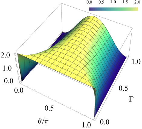
Figure 1: (Color online) Qubit MA: the quantum tradeoff ${\rm Tr}[{\bm{Q}}{\bm{H}}^{-1}]$ as a function of $\theta$ and $\Gamma$ is shown at $\gamma=\pi/2$. The tradeoff can reach its maximum (= 2 in this case) for a suitable choice of $\theta$, i.e., $\theta=\pi/2,$ regardless of $\Gamma$.

For a suitable choice of MA state ($\theta=\pi/2$), the quantum tradeoff ${\rm Tr}[{\bm{Q}}{\bm{H}}^{-1}]$ can reach two regardless of $\Gamma$. This result implies that all the ratios ${\bm{Q}}_{\alpha\alpha}/{\bm{H}}_{\alpha\alpha},\ \alpha=\phi,\Gamma,$ simultaneously reach one, or ${\bm{Q}}$ approaches ${\bm{H}}$. Therefore, we should be possible to estimate both the phase and its fluctuation with the quantum-limit precision simultaneously.

We note, however, that it is not possible to construct a set of POVMs corresponding to $\hat{L}_{\phi}^{(\jmath)}$ and $\hat{L}_{\Gamma}^{(\jmath)}$ because the sensor is in mixed state. See, Sec. II.3. We believe that collective measurements, such as Refs. Vidrighin5 ; Rafal2020 ; Ragy94 , may provide the way to measure $\phi$ and $\Gamma$ with ultimate precision simultaneously.

IV Discussion and Conclusion

We analyze simultaneous multiple parameter estimations in postselection measurements in terms of tradeoff relations. We first derive classical and quantum Cramér-Rao lower bounds and discuss the tradeoffs in the postselection measurements in general. Then, we discuss simultaneous measurements of phase and its fluctuation with a discrete qubit MA. This example confirms our general results. We found that the tradeoffs can be saturated and thus all the parameters should, in principle, be possible to attain the ultimate precision simultaneously. We note, however, that it is not possible to construct a set of POVMs for such measurements because the sensor is in mixed state. We have not yet been successful to propose a concrete measurement procedure and this is our future work.

We conclude this work by pointing out that postselection measurements can provide another way to control a measurement through an extra freedom of postselected states and the MA state.

Appendix A Proof of Cramér-Rao bounds

We will prove Eq. (10) here.

A.1 Proof of $\bm{F}\leq\bm{Q}$

Let us recast $\bm{F}$ and $\bm{Q}$ as $\bm{F}=\sum_{\jmath}\bm{F}^{(\jmath)}$ and $\bm{Q}=\sum_{\jmath}\bm{Q}^{(\jmath)}$. Then, we can prove that $\bm{F}^{(\jmath)}\leq\bm{Q}^{(\jmath)}$, $\forall\jmath$.

$\bm{F}^{(\jmath)}\leq\bm{Q}^{(\jmath)}$ means $\bm{u}^{\intercal}[\bm{F}^{(\jmath)}]\bm{u}\leq\bm{u}^{\intercal}[\bm{Q}^{(\jmath)}]\bm{u}$ for arbitrary $d$-dimensional real vectors $\bm{u}$ Pezze119 . We first rewrite the elements of $\bm{F}^{(\jmath)}$ as ${\bm{F}}^{(\jmath)}_{\alpha\beta}=w^{(\jmath)}\sum_{\mu}[{\bm{F}}(\mu|\jmath)]_{\alpha\beta}$, where $[{\bm{F}}(\mu|\jmath)]_{\alpha\beta}$ is defined by

$$[{\bm{F}}(\mu|\jmath)]_{\alpha\beta} \equiv\dfrac{1}{P(\mu|\jmath)}\dfrac{\partial P(\mu|\jmath)}{\partial\phi_{\alpha}}\dfrac{\partial P(\mu|\jmath)}{\partial\phi_{\beta}}$$

$$=\dfrac{1}{{\rm Tr_{m}}[\rho^{(\jmath)}_{\rm m}\hat{\Pi}_{\mu}]}\dfrac{\partial{\rm Tr_{m}}[\rho^{(\jmath)}_{\rm m}\hat{\Pi}_{\mu}]}{\partial\phi_{\alpha}}\dfrac{\partial{\rm Tr_{m}}[\rho^{(\jmath)}_{\rm m}\hat{\Pi}_{\mu}]}{\partial\phi_{\beta}},$$ (A.1)

where we have used $P(\mu|\jmath)={\rm Tr_{m}}[\rho^{(\jmath)}_{\rm m}\hat{\Pi}_{\mu}]$. Using the SLD, $\partial_{k}\rho^{(\jmath)}_{\rm m}=(\hat{L}^{(\jmath)}_{k}\rho^{(\jmath)}_{\rm m}+\rho^{(\jmath)}_{\rm m}\hat{L}^{(\jmath)}_{k})/2$, where $\partial_{k}\equiv\partial/\partial\phi_{k}$ and $k=\alpha,\beta$, we have

$$\dfrac{\partial{\rm Tr_{m}}[\rho^{(\jmath)}_{\rm m}\hat{\Pi}_{\mu}]}{\partial\phi_{k}} ={\rm Tr_{m}}\Bigl{[}\dfrac{\partial\rho^{(\jmath)}_{\rm m}\hat{\Pi}_{\mu}}{\partial\phi_{k}}\Bigr{]}$$

$$=\dfrac{1}{2}\Bigl{\{}{\rm Tr_{m}}\bigl{[}\hat{L}^{(\jmath)}_{k}\rho^{(\jmath)}_{\rm m}\hat{\Pi}_{\mu}\bigr{]}+{\rm Tr_{m}}\bigl{[}\rho^{(\jmath)}_{\rm m}\hat{L}^{(\jmath)}_{k}\hat{\Pi}_{\mu}\bigr{]}\Bigr{\}}$$

$$={\rm Re}\Bigl{[}{\rm Tr_{m}}\bigl{[}\rho^{(\jmath)}_{\rm m}\hat{\Pi}_{\mu}\hat{L}^{(\jmath)}_{k}\bigr{]}\Bigr{]}.$$ (A.2)

The following equality is employed here.

$${\rm Tr_{m}}\bigl{[}\rho^{(\jmath)}_{\rm m}\hat{L}^{(\jmath)}_{k}\hat{\Pi}_{\mu}\bigr{]}={\rm Tr_{m}}\bigl{[}\hat{L}^{(\jmath)}_{k}\hat{\Pi}_{\mu}\rho^{(\jmath)}_{\rm m}\bigr{]}=\Bigl{[}{\rm Tr_{m}}\bigl{[}\rho^{(\jmath)}_{\rm m}\hat{\Pi}_{\mu}\hat{L}^{(\jmath)}_{k}\bigr{]}\Bigr{]}^{*}$$ (A.3)

We calculate as follows Yang2018 :

$$\sum_{\alpha\beta}u_{\alpha}[\bm{F}(\mu|\jmath)]_{\alpha\beta}\ u_{\beta} =\dfrac{\Bigl{[}{\rm ReTr_{m}}\bigl{[}\rho^{(\jmath)}_{\rm m}\hat{\Pi}_{\mu}\sum_{\alpha}u_{\alpha}\hat{L}^{(\jmath)}_{\alpha}\bigr{]}\Bigr{]}^{2}}{{\rm Tr_{m}}[\rho^{(\jmath)}_{\rm m}\hat{\Pi}_{\mu}]}$$

$$\overset{(a)}{\leq}\dfrac{\Bigl{|}{\rm Tr_{m}}\bigl{[}\rho^{(\jmath)}_{\rm m}\hat{\Pi}_{\mu}\sum_{\alpha}u_{\alpha}\hat{L}^{(\jmath)}_{\alpha}\bigr{]}\Bigr{|}^{2}}{{\rm Tr_{m}}[\rho^{(\jmath)}_{\rm m}\hat{\Pi}_{\mu}]}$$

$$\overset{(b)}{\leq}\sum_{\alpha\beta}u_{\alpha}u_{\beta}{\rm Tr_{m}}\bigl{[}\rho^{(\jmath)}_{\rm m}\hat{L}^{(\jmath)}_{\alpha}\hat{\Pi}_{\mu}\hat{L}^{(\jmath)}_{\beta}\bigr{]}$$

$$\overset{(c)}{=}\dfrac{1}{2}\sum_{\alpha\beta}u_{\alpha}{\rm Tr_{m}}\bigl{[}\rho^{(\jmath)}_{\rm m}(\hat{L}^{(\jmath)}_{\alpha}\hat{\Pi}_{\mu}\hat{L}^{(\jmath)}_{\beta}+\hat{L}^{(\jmath)}_{\beta}\hat{\Pi}_{\mu}\hat{L}^{(\jmath)}_{\alpha})\bigr{]}u_{\beta}$$

$$\overset{(d)}{=}\sum_{\alpha\beta}u_{\alpha}[\bm{Q}(\mu|\jmath)]_{\alpha\beta}\ u_{\beta}.$$ (A.4)

We employs the followings. (a) Using an inequality $[{\rm Re}(z)]^{2}\leq|z|^{2}$ for a complex number $z$. (b) Using the Cauchy-Schwartz inequality $|{\rm Tr}(\hat{A}^{\dagger}\hat{B})|^{2}\leq{\rm Tr}(\hat{A}^{\dagger}\hat{A}){\rm Tr}(\hat{B}^{\dagger}\hat{B})$, where $\hat{A}\equiv\sqrt{\hat{\Pi}_{\mu}}\sqrt{\rho_{\rm m}^{(\jmath)}}$ and $\hat{B}\equiv\sum_{\alpha}\sqrt{\hat{\Pi}_{\mu}}u_{\alpha}\hat{L}^{(\jmath)}_{\alpha}\sqrt{\rho_{\rm m}^{(\jmath)}}$. (c) Using the symmetry of the indices $\alpha$ and $\beta$. (d) Remembering the definition of $\bm{Q}^{(\jmath)}$ ($[\bm{Q}(\mu|\jmath)]_{\alpha\beta}\equiv{\rm Tr_{m}}\bigl{[}\rho^{(\jmath)}_{\rm m}\frac{\hat{L}^{(\jmath)}_{\alpha}\hat{\Pi}_{\mu}\hat{L}^{(\jmath)}_{\beta}+\hat{L}^{(\jmath)}_{\beta}\hat{\Pi}_{\mu}\hat{L}^{(\jmath)}_{\alpha}}{2}\bigr{]}$). By taking the sum over $\mu$, we obtain

$$\sum_{\alpha\beta}u_{\alpha}[\bm{F}^{(\jmath)}]_{\alpha\beta}\ u_{\beta}\leq\sum_{\alpha\beta}u_{\alpha}[\bm{Q}^{(\jmath)}]_{\alpha\beta}\ u_{\beta}.$$ (A.5)

Or, we obtain $\bm{F}^{(\jmath)}\leq\bm{Q}^{(\jmath)}$, $\forall\jmath$, and thus, we obtain $\bm{F}\leq\bm{Q}$. $\Box$

A.2 Proof of $\bm{Q}\leq\bm{H}$

We next prove the inequality $\bm{Q}\leq\bm{H}$. Let us denote $\bm{Q}_{\rm sm}$ the Fisher information matrix obtained from the joint measurements of the sensor-MA. We note that $\bm{Q}_{\rm sm}=\bm{H}$ since no information can be gained or lost after the sensor-MA interaction. We, therefore, will prove that $\bm{Q}\leq\bm{Q}_{\rm sm}$. Remind that $\bm{Q}=\sum_{\jmath}\bm{Q}^{(\jmath)}$. Assume that the existence of optimal measurement is a set of POVMs $\{\Pi^{(\jmath)}_{k}\}$ for $k$ outcomes in the MA and the corresponding probability is $P(k|\jmath)$, then we have

$$\bm{Q}^{(\jmath)}_{\alpha\beta}=w^{(\jmath)}\sum_{k}\dfrac{1}{P(k|\jmath)}\dfrac{\partial P(k|\jmath)}{\partial\phi_{\alpha}}\dfrac{\partial P(k|\jmath)}{\partial\phi_{\beta}}.$$ (A.6)

The corresponding optimal POVM measurement of the joint state is given by a set $\bigl{\{}\{\rho_{\rm s,f}^{(1)}\otimes\Pi^{(1)}_{k_{1}}\},\{(\rho_{\rm s,f}^{(2)})\otimes\Pi^{(2)}_{k_{2}}\},\{(\rho_{\rm s,f}^{(3)})\otimes\Pi^{(3)}_{k_{3}}\},...\bigr{\}}$. The probabilities are $w^{(\jmath)}P(k_{i}|\jmath)$, for $\jmath=1,2,...$. The Fisher information corresponds to the joint sensor-MA state is

$$\bm{Q}_{\rm sm} =\sum_{\jmath}\sum_{k_{\jmath}}\dfrac{1}{w^{(\jmath)}P(k_{\jmath}|{\jmath})}\dfrac{\partial[w^{(\jmath)}P(k_{\jmath}|{\jmath})]}{\partial\phi_{\alpha}}\dfrac{\partial[w^{(\jmath)}P(k_{\jmath}|{\jmath})]}{\partial\phi_{\beta}}$$

$$=\sum_{\jmath}\sum_{k_{\jmath}}\dfrac{1}{w^{(\jmath)}P(k_{\jmath}|{\jmath})}\Bigl{[}\dfrac{\partial w^{(\jmath)}}{\partial\phi_{\alpha}}P(k_{\jmath}|\jmath)+w^{(\jmath)}\dfrac{\partial P(k_{\jmath}|\jmath)}{\partial\phi_{\alpha}}\Bigr{]}\Bigl{[}\dfrac{\partial w^{(\jmath)}}{\partial\phi_{\beta}}P(k_{\jmath}|\jmath)+w^{(\jmath)}\dfrac{\partial P(k_{\jmath}|\jmath)}{\partial\phi_{\beta}}\Bigr{]}$$

$$=\sum_{\jmath}w^{(\jmath)}\sum_{k_{\jmath}}\dfrac{1}{P(k_{\jmath}|{\jmath})}\dfrac{\partial P(k_{\jmath}|{\jmath})}{\partial\phi_{\alpha}}\dfrac{\partial P(k_{\jmath}|{\jmath})}{\partial\phi_{\beta}}+\mathcal{F}$$

$$=\sum_{\jmath}\bm{Q}^{(\jmath)}+\mathcal{F}$$

$$\geq\bm{Q}\;,$$ (A.7)

where $\mathcal{F}$ is given by

$$\mathcal{F}=\sum_{\jmath}\Bigl{\{}\dfrac{1}{w^{(\jmath)}}\dfrac{\partial w^{(\jmath)}}{\partial\phi_{\alpha}}\dfrac{\partial w^{(\jmath)}}{\partial\phi_{\beta}}+\sum_{k_{\jmath}}\Bigl{(}\dfrac{\partial w^{(\jmath)}}{\partial\phi_{\alpha}}\dfrac{\partial P(k_{\jmath}|{\jmath})}{\partial\phi_{\beta}}+\dfrac{\partial w^{(\jmath)}}{\partial\phi_{\beta}}\dfrac{\partial P(k_{\jmath}|{\jmath})}{\partial\phi_{\alpha}}\Bigr{)}\Bigr{\}}.$$ (A.8)

Note that $\mathcal{F}$ is the classical Fisher information contributed by all the postselection probabilities, hence it is non-negative. As a result, we have $\bm{Q}\leq\bm{H}.\ \Box$

Appendix B Continuous Gaussian MA

In this Appendix, we provide another example for the simultaneous estimation of phase and phase fluctuation via a continuous measurement apparatus (MA). We consider the continuous Gaussian MA with a zero-mean in position $x$

$$|\xi\rangle=\int dx\dfrac{1}{(2\pi\sigma^{2})^{1/4}}\exp\Bigl{(}-\dfrac{x^{2}}{4\sigma^{2}}\Bigr{)}|x\rangle,$$

where we take the natural unit so that $\hbar=1$. This MA is widely used in weak measurement studies Aharonov60 ; Ritchie66 ; Hosten319 ; Dixon102 ; Brunner105 ; Zilberberg106 ; Gorodetski109 and is a prototype for discussing the postselection measurements. $|\xi\rangle$ is equivalently given by

$$|\xi\rangle=\int dp\Bigl{(}\dfrac{2\sigma^{2}}{\pi}\Bigr{)}^{1/4}\exp(-p^{2}\sigma^{2})|p\rangle,$$ (B.1)

where $p$ is momentum.

We consider the unitary evolution $\hat{U}_{\rm sm}=\exp(-ig\sigma_{z}\otimes\hat{p})$ as a sensor-MA interaction, where $\hat{p}$ is a momentum operator, $\hat{p}=-i\partial_{x}$. Throughout this paper, we fix $g=\pi/2$ for simplicity. The postselected states are chosen the same as in the case of the qubit MA. Note that in this case we also have two orthonormal postselected states, i.e., $\jmath=1,2$. The probability of postselection, $w^{(\jmath)}$, is calculated according to Eq. (3) where $I_{\rm m}$ is replaced with $\int_{-\infty}^{\infty}dp^{\prime}|p^{\prime}\rangle\langle p^{\prime}|$.

$$w^{(\jmath)} =\Bigl{(}\dfrac{2\sigma}{\pi}\Bigr{)}^{\nicefrac{{1}}{{2}}}\int dp\ e^{-2p^{2}\sigma^{2}}\ {\rm Tr}_{\rm s}\bigl{[}\rho_{\rm s,f}^{(\jmath)}\hat{U}_{\rm s}\rho^{\prime}_{\rm s,i}\hat{U}^{\dagger}_{\rm s}\bigr{]}$$

$$=\dfrac{1}{2}\Bigl{(}1+e^{-\Gamma^{2}-\frac{\pi^{2}}{8\sigma^{2}}}\cos\phi\sin\gamma\Bigr{)},$$ (B.2)

where $\hat{U}_{\rm s}=\exp(-i\frac{\pi}{2}p\sigma_{z})$. Note that $p$ in $\hat{U}_{\rm s}$ is not an operator.

We next decompose the sensor state as

$$\rho^{\prime}_{\rm s,i}=\sum_{k}\lambda_{k}|\psi_{k}\rangle\langle\psi_{k}|=\lambda_{1}|\psi_{1}\rangle\langle\psi_{1}|+\lambda_{2}|\psi_{2}\rangle\langle\psi_{2}|,$$ (B.3)

where $\lambda_{k}$ and $|\psi_{k}\rangle$ ($k=1,2$), are eigenvalues and eigenstates of $\rho^{\prime}_{\rm s,i}$, respectively. Substituting $\rho^{\prime}_{\rm s,i}$ into Eq. (4), we have

$$\rho^{(\jmath)}_{\rm m}=\sum_{k=1}^{2}\dfrac{\lambda_{k}\hat{B}_{k}^{(\jmath)}|\xi\rangle\langle\xi|[\hat{B}_{k}^{(\jmath)}]^{\dagger}}{w^{(\jmath)}}=\sum_{k=1}^{2}\lambda_{k}|\xi^{(\jmath)}_{k}\rangle\langle\xi^{(\jmath)}_{k}|,$$ (B.4)

where $\hat{B}_{k}^{(\jmath)}=\bigl{(}\langle\psi_{\rm s,f}^{(\jmath)}|\otimes\hat{I}_{\rm m}\bigr{)}\hat{U}_{\rm sm}\bigl{(}|\psi_{k}\rangle\otimes\hat{I}_{\rm m}\bigr{)}$. We also define $|\xi^{(\jmath)}_{k}\rangle\equiv\hat{B}_{k}^{(\jmath)}|\xi\rangle/\sqrt{w^{(\jmath)}}$. We emphasize that, in general, $\{|\xi^{(\jmath)}_{k}\rangle\}$ are not orthogonal. In the case of $\gamma=\pi/2$ and $\phi\rightarrow 0$, however, we have $\langle\xi^{(\jmath)}_{1}|\xi^{(\jmath)}_{2}\rangle=\langle\xi^{(\jmath)}_{2}|\xi^{(\jmath)}_{1}\rangle=0$ (see Appendix C). We define $N_{k}^{(\jmath)}\equiv\langle\xi^{(\jmath)}_{k}|\xi^{(\jmath)}_{k}\rangle,k=1,2$.

We first show that Tr${}_{\rm m}[\rho^{(\jmath)}_{\rm m}[\hat{L}^{(\jmath)}_{\phi},\hat{L}^{(\jmath)}_{\Gamma}]]$ is given as

$${\rm Tr}_{\rm m}\bigl{[}\rho^{(\jmath)}_{\rm m}[\hat{L}^{(\jmath)}_{\phi},\hat{L}^{(\jmath)}_{\Gamma}]\bigr{]}=4\sum_{k,l=1}^{2}\Bigl{(}\dfrac{\lambda_{k}}{N_{l}^{(\jmath)}}-\dfrac{\lambda_{l}}{N_{k}^{(\jmath)}}\Bigr{)}\dfrac{\langle\xi^{(\jmath)}_{k}|\partial_{\phi}\rho_{\rm m}^{(\jmath)}|\xi^{(\jmath)}_{l}\rangle\langle\xi^{(\jmath)}_{l}|\partial_{\Gamma}\rho_{\rm m}^{(\jmath)}|\xi^{(\jmath)}_{k}\rangle}{(\lambda_{k}N_{k}^{(\jmath)}+\lambda_{l}N_{l}^{(\jmath)})^{2}},$$ (B.5)

in the Gaussian MA case. Then ${\rm Tr}_{\rm m}\bigl{[}\rho^{(\jmath)}_{\rm m}[\hat{L}^{(\jmath)}_{\phi},\hat{L}^{(\jmath)}_{\Gamma}]\bigr{]}=0$ when $\gamma=\pi/2$ and $\phi\to 0$. (See the detailed calculation in Appendix C.) Using also collective measurements, for example, $\bm{Q}$ may be achieved or the pQCRB can satisfy.

We analytically obtain $\bm{Q}$ with the conditions that $\gamma=\pi/2$ and $\phi\to 0$, as follows.

$$\bm{Q}^{(\jmath)}_{\alpha\beta}=4w^{(\jmath)}\sum_{k,l=1}^{2}\dfrac{\lambda_{k}}{N_{l}^{(\jmath)}}\dfrac{\langle\xi^{(\jmath)}_{k}|\partial_{\alpha}\rho^{(\jmath)}_{\rm m}|\xi^{(\jmath)}_{l}\rangle\langle\xi^{(\jmath)}_{l}|\partial_{\beta}\rho^{(\jmath)}_{\rm m}|\xi^{(\jmath)}_{k}\rangle}{(\lambda_{k}N_{k}^{(\jmath)}+\lambda_{l}N_{l}^{(\jmath)})^{2}},$$ (B.6)

where we have defined $\bm{Q}^{(\jmath)}$, $\jmath=1,2$ are the pQFIMs for the two orthonormal postselected states, respectively. See Appendix C for detailed calculations. Finally, we have the total pQFIM, $\bm{Q}=\bm{Q}^{(1)}+\bm{Q}^{(2)}$. Straightforward calculations give $\bm{Q}$ as

$$\bm{Q}_{\phi\phi} =\dfrac{e^{-\Gamma^{2}}}{\cosh\Gamma^{2}+\coth\bigl{(}\frac{\pi^{2}}{8\sigma^{2}}\bigr{)}\sinh\Gamma^{2}},$$ (B.7)

$$\bm{Q}_{\Gamma\Gamma} =2\Gamma^{2}\ \text{csch}\Gamma^{2}\ \text{csch}\bigl{(}\Gamma^{2}+\frac{\pi^{2}}{8\sigma^{2}}\bigr{)}\sinh\bigr{(}\frac{\pi^{2}}{8\sigma^{2}}\bigr{)},$$ (B.8)

$$\bm{Q}_{\phi\Gamma} =\bm{Q}_{\Gamma\phi}=0.$$ (B.9)

where $\text{csch }x=2/(e^{x}-e^{-x})$.

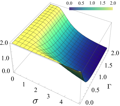
Figure 2: (Color online) Continuous Gaussian MA: the quantum tradeoff ${\rm Tr}[{\bm{Q}}{\bm{H}}^{-1}]$ as a function of $\sigma$ and $\Gamma$ is shown at $\gamma=\pi/2$. The tradeoff can reach its maximum (= 2 in this case) for a suitable choice of $\sigma$, i.e., $\sigma<1$ (weak measurement) regardless of $\Gamma$.

We now calculate the quantum tradeoff. By using Eqs. (B.7, B.8) and Eq. (16), the quantum tradeoff, ${\rm Tr}[{\bm{Q}}{\bm{H}}^{-1}]$, in the simultaneous estimation of $\phi$ and $\Gamma$ reads

$${\rm Tr}\bigl{[}{\bm{Q}}{\bm{H}}^{-1}\bigr{]} =\dfrac{{\bm{Q}}_{\phi\phi}}{{\bm{H}}_{\phi\phi}}+\dfrac{{\bm{Q}}_{\Gamma\Gamma}}{{\bm{H}}_{\Gamma\Gamma}}$$

$$=2e^{\Gamma^{2}}\text{csch}\bigl{(}\Gamma^{2}+\frac{\pi^{2}}{8\sigma^{2}}\bigr{)}\sinh\bigl{(}\frac{\pi^{2}}{8\sigma^{2}}\bigr{)}.$$ (B.10)

The result is summarized in Fig. 2. The quantum tradeoff can reach the maximum of two for small $\sigma$ regardless of $\Gamma$, which is consistent with ${\rm Tr}_{\rm m}\bigl{[}\rho^{(\jmath)}_{\rm m}[\hat{L}^{(\jmath)}_{\phi},\hat{L}^{(\jmath)}_{\Gamma}]\bigr{]}=0$. This result implies that all the ratios ${\bm{Q}}_{\alpha\alpha}/{\bm{H}}_{\alpha\alpha},\ \alpha=\phi,\Gamma,$ simultaneously reach one. It also means that it is not impossible to estimate both the phase and its fluctuation with the quantum-limit precision simultaneously. This is the benefit of the postselection measurement scheme in which an extra freedom of MA, $\sigma$ in this case, is introduced. We also observe that ${\bm{Q}}_{\phi\phi}/{\bm{H}}_{\phi\phi}={\bm{Q}}_{\Gamma\Gamma}/{\bm{H}}_{\Gamma\Gamma}$, or they can always attain the same precision: It is known as a Fisher-symmetric informationally complete (FSIC) Li116 .

Appendix C Detailed Calculation in the case of Continuous Gaussian MA

C.1 Calculation of ${\rm Tr}[\rho[L_{\alpha},L_{\beta}]]$ in general

Let us first calculate the SLD operator corresponding to an arbitrary $\rho$ with the following Lyapunov representation Paris7

$$\hat{L}_{\alpha}=2\int_{0}^{\infty}dte^{-t\rho}\bigl{(}\partial_{\alpha}\rho\bigr{)}e^{-t\rho},$$ (C.1)

with $\rho=\sum_{k}\lambda_{k}|\xi_{k}\rangle\langle\xi_{k}|$, where $\langle\xi_{k}|\xi_{l}\rangle=0$ for $k\neq l$, and $\langle\xi_{k}|\xi_{k}\rangle=N_{k}$. Evaluating the exponential $e^{-t\rho}$, we have

$$e^{-t\rho}=\sum_{k}\dfrac{e^{-t\lambda_{k}N_{k}}}{N_{k}}|\xi_{k}\rangle\langle\xi_{k}|.$$ (C.2)

Substituting Eq. (C.2) into Eq. (C.1), we obtain

$$\hat{L}_{\alpha}=2\sum_{kl}\dfrac{1}{N_{k}N_{l}}\ \dfrac{\langle\xi_{k}|\partial_{\alpha}\rho|\xi_{l}\rangle}{\lambda_{k}N_{k}+\lambda_{l}N_{l}}\ |\xi_{k}\rangle\langle\xi_{l}|.$$ (C.3)

We next evaluate the term $\hat{L}_{\alpha}\hat{L}_{\beta}$ as

$$\hat{L}_{\alpha}\hat{L}_{\beta}=4\sum_{kll^{\prime}}\dfrac{1}{N_{k}N_{l}N_{l^{\prime}}}\ \dfrac{\langle\xi_{k}|\partial_{\alpha}\rho|\xi_{l}\rangle}{\lambda_{k}N_{k}+\lambda_{l}N_{l}}\ \dfrac{\langle\xi_{l}|\partial_{\beta}\rho|\xi_{l^{\prime}}\rangle}{\lambda_{l}N_{l}+\lambda_{l^{\prime}}N_{l^{\prime}}}\ |\xi_{k}\rangle\langle\xi_{l^{\prime}}|.$$ (C.4)

Using $\rho=\sum_{n}\lambda_{n}|\xi_{n}\rangle\langle\xi_{n}|$, we have

$$\rho\hat{L}_{\alpha}\hat{L}_{\beta}=4\sum_{kll^{\prime}}\dfrac{\lambda_{k}}{N_{l}N_{l^{\prime}}}\ \dfrac{\langle\xi_{k}|\partial_{\alpha}\rho|\xi_{l}\rangle}{\lambda_{k}N_{k}+\lambda_{l}N_{l}}\ \dfrac{\langle\xi_{l}|\partial_{\beta}\rho|\xi_{l^{\prime}}\rangle}{\lambda_{l}N_{l}+\lambda_{l^{\prime}}N_{l^{\prime}}}\ |\xi_{k}\rangle\langle\xi_{l^{\prime}}|.$$ (C.5)

Taking the trace, we obtain

$${\rm Tr}[\rho\hat{L}_{\alpha}\hat{L}_{\beta}]=4\sum_{kl}\dfrac{\lambda_{k}}{N_{l}}\ \dfrac{\langle\xi_{k}|\partial_{\alpha}\rho|\xi_{l}\rangle\langle\xi_{l}|\partial_{\beta}\rho|\xi_{k}\rangle}{(\lambda_{k}N_{k}+\lambda_{l}N_{l})^{2}}.$$ (C.6)

Similarly, we have

$${\rm Tr}[\rho\hat{L}_{\beta}\hat{L}_{\alpha}]=4\sum_{kl}\dfrac{\lambda_{l}}{N_{k}}\ \dfrac{\langle\xi_{k}|\partial_{\alpha}\rho|\xi_{l}\rangle\langle\xi_{l}|\partial_{\beta}\rho|\xi_{k}\rangle}{(\lambda_{k}N_{k}+\lambda_{l}N_{l})^{2}}.$$ (C.7)

Finally, we obtain

$${\rm Tr}\bigl{[}\rho[\hat{L}_{\alpha},\hat{L}_{\beta}]\bigr{]}=4\sum_{kl}\Bigl{(}\dfrac{\lambda_{k}}{N_{l}}-\dfrac{\lambda_{l}}{N_{k}}\Bigr{)}\ \dfrac{\langle\xi_{k}|\partial_{\alpha}\rho|\xi_{l}\rangle\langle\xi_{l}|\partial_{\beta}\rho|\xi_{k}\rangle}{(\lambda_{k}N_{k}+\lambda_{l}N_{l})^{2}},$$ (C.8)

where

$$\partial_{\alpha}\rho=\sum_{n}\Bigl{(}\partial_{\alpha}\lambda_{n}|\xi_{n}\rangle\langle\xi_{n}|+\lambda_{n}|\partial_{\alpha}\xi_{n}\rangle\langle\xi_{n}|+\lambda_{n}|\xi_{n}\rangle\langle\partial_{\alpha}\xi_{n}|\Bigr{)}.$$ (C.9)

C.2 Calculation of ${\rm Tr}[\rho[L_{\alpha},L_{\beta}]]$ in our example

Let us now apply the above calculations to our case of the continuous Gaussian MA where ${\rm Tr}[\rho[L_{\alpha},L_{\beta}]]$ now becomes ${\rm Tr}_{\rm m}[\rho_{\rm m}^{(\jmath)}[L_{\phi}^{(\jmath)},L_{\Gamma}^{(\jmath)}]]$ for $\jmath=1,2$. We start from the sensor state given in Eq. (15) and decompose it into the sum of the eigenstates as in Eq. (B.3). We obtain

$$\lambda_{1}=\dfrac{1}{2}(1-e^{-\Gamma^{2}})\ \text{and }\lambda_{2}=\dfrac{1}{2}(e^{-\Gamma^{2}}+1),$$ (C.10)

$$|\psi_{1}\rangle=\dfrac{1}{\sqrt{2}}\begin{pmatrix}-e^{-i\phi}\\ 1\end{pmatrix}\ \text{and }|\psi_{2}\rangle=\dfrac{1}{\sqrt{2}}\begin{pmatrix}e^{-i\phi}\\ 1\end{pmatrix}.$$ (C.11)

We next calculate $|\xi_{k}^{(\jmath)}\rangle$ which is defined by:

$$|\xi_{k}^{(\jmath)}\rangle =\dfrac{\hat{B}_{k}^{(\jmath)}}{\sqrt{w^{(\jmath)}}}|\xi\rangle,$$ (C.12)

where $\hat{B}_{k}^{(\jmath)}=\bigl{(}\langle\psi_{\rm s,f}^{(\jmath)}|\otimes\hat{I}_{\rm m}\bigr{)}\hat{U}_{\rm sm}\bigl{(}|\psi_{k}\rangle\otimes\hat{I}_{\rm m}\bigr{)}$. We show explicitly

$$\hat{B}_{k}^{(\jmath)} =\Bigl{(}\langle\psi_{\rm s,f}^{(\jmath)}|\otimes\int dp|p\rangle\langle p|\Bigr{)}e^{-ig\sigma_{z}\otimes\hat{p}}\Bigl{(}|\psi_{k}\rangle\otimes\int dp^{\prime}|p^{\prime}\rangle\langle p^{\prime}\Bigr{)}$$

$$=\int dp\ \langle\psi_{\rm s,f}^{(\jmath)}|e^{-igp\sigma_{z}}|\psi_{k}\rangle|p\rangle\langle p|.$$ (C.13)

Then we have

$$\hat{B}_{1}^{(1)} =\int dp\ \Bigl{[}\dfrac{e^{-\frac{i(p\pi+2\phi)}{2}}\bigl{(}e^{i(p\pi+\phi)}\cos\frac{\gamma}{2}-\sin\frac{\gamma}{2}\bigr{)}}{\sqrt{2}}\Bigr{]}|p\rangle\langle p|,$$ (C.14)

$$\hat{B}_{2}^{(1)} =\int dp\ \Bigl{[}\dfrac{e^{-\frac{i(p\pi+2\phi)}{2}}\bigl{(}e^{i(p\pi+\phi)}\cos\frac{\gamma}{2}+\sin\frac{\gamma}{2}\bigr{)}}{\sqrt{2}}\Bigr{]}|p\rangle\langle p|,$$ (C.15)

$$\hat{B}_{1}^{(2)} =\int dp\ \Bigl{[}-\dfrac{e^{-\frac{i(p\pi+2\phi)}{2}}\bigl{(}\cos\frac{\gamma}{2}+e^{i(p\pi+\phi)}\sin\frac{\gamma}{2}\bigr{)}}{\sqrt{2}}\Bigr{]}|p\rangle\langle p|,$$ (C.16)

$$\hat{B}_{2}^{(2)} =\int dp\ \Bigl{[}\dfrac{e^{-\frac{i(p\pi+2\phi)}{2}}\bigl{(}\cos\frac{\gamma}{2}-e^{i(p\pi+\phi)}\sin\frac{\gamma}{2}\bigr{)}}{\sqrt{2}}\Bigr{]}|p\rangle\langle p|.$$ (C.17)

Substituting into Eq. (C.12) we obtain

$$|\xi_{k}^{(\jmath)}\rangle=\Bigl{(}\dfrac{2\sigma^{2}}{\pi}\Bigr{)}^{1/4}\dfrac{1}{\sqrt{w^{(\jmath)}}}\int dp\ e^{-p^{2}\sigma^{2}}\overline{B_{k}^{(\jmath)}}|p\rangle,$$ (C.18)

where we have used $\langle p|\xi\rangle=(2\sigma^{2}/\pi)^{1/4}\exp(-p^{2}\sigma^{2})$ and $\overline{B_{k}^{(\jmath)}}$ are given by $[*]$ in Eqs. (C.14-C.17) above.

We calculate $\langle\xi_{1}^{(\jmath)}|\xi_{2}^{(\jmath)}\rangle$. For $\phi\to 0$, we have

$$\langle\xi_{1}^{(1)}|\xi_{2}^{(1)}\rangle=\dfrac{e^{\Gamma^{2}+\frac{\pi^{2}}{8\sigma^{2}}}\cos\gamma}{e^{\Gamma^{2}+\frac{\pi^{2}}{8\sigma^{2}}}+\sin\gamma},\ \text{and }\langle\xi_{1}^{(2)}|\xi_{2}^{(2)}\rangle=-\dfrac{e^{\Gamma^{2}+\frac{\pi^{2}}{8\sigma^{2}}}\cos\gamma}{e^{\Gamma^{2}+\frac{\pi^{2}}{8\sigma^{2}}}-\sin\gamma}.$$ (C.19)

Then, $|\xi_{1}^{(\jmath)}\rangle$ and $|\xi_{2}^{(\jmath)}\rangle$ are orthonormal when $\gamma=\pi/2$. We select $\gamma=\pi/2$ hereafter. We next calculate the normalized constants $N_{k}^{(\jmath)}=\langle\xi_{k}^{(\jmath)}|\xi_{k}^{(\jmath)}\rangle$ which are given as

$$N_{1}^{(1)}=1-\dfrac{1+e^{\Gamma^{2}}}{1+e^{\Gamma^{2}+\frac{\pi^{2}}{8\sigma^{2}}}},\ \text{and }N_{2}^{(1)}=1+\dfrac{-1+e^{\Gamma^{2}}}{1+e^{\Gamma^{2}+\frac{\pi^{2}}{8\sigma^{2}}}},$$ (C.20)

and

$$N_{1}^{(2)}=1-\dfrac{1+e^{\Gamma^{2}}}{1-e^{\Gamma^{2}+\frac{\pi^{2}}{8\sigma^{2}}}},\ \text{and }N_{2}^{(2)}=1+\dfrac{-1+e^{\Gamma^{2}}}{1-e^{\Gamma^{2}+\frac{\pi^{2}}{8\sigma^{2}}}}.$$ (C.21)

Finally, we calculate Eq. (C.8) which is recast as

$${\rm Tr}_{\rm m}\bigl{[}\rho_{\rm m}^{(\jmath)}[\hat{L}_{\phi}^{(\jmath)},\hat{L}_{\Gamma}^{(\jmath)}]\bigr{]}=4\sum_{k,l=1}^{2}\Bigl{(}\dfrac{\lambda_{k}}{N_{l}^{(\jmath)}}-\dfrac{\lambda_{l}}{N_{k}^{(\jmath)}}\Bigr{)}\ \dfrac{\langle\xi_{k}^{(\jmath)}|\partial_{\phi}\rho_{\rm m}^{(\jmath)}|\xi_{l}^{(\jmath)}\rangle\langle\xi_{l}^{(\jmath)}|\partial_{\Gamma}\rho_{\rm m}^{(\jmath)}|\xi_{k}^{(\jmath)}\rangle}{(\lambda_{k}N_{k}^{(\jmath)}+\lambda_{l}N_{l}^{(\jmath)})^{2}}.$$ (C.22)

First we derive Eq. (C.9):

$$\partial_{\phi}\rho_{\rm m}^{(\jmath)}=\sum_{n=1}^{2}\Bigl{(}\partial_{\phi}\lambda_{n}|\xi_{n}^{(\jmath)}\rangle\langle\xi_{n}^{(\jmath)}|+\lambda_{n}|\partial_{\phi}\xi_{n}^{(\jmath)}\rangle\langle\xi_{n}^{(\jmath)}|+\lambda_{n}|\xi_{n}^{(\jmath)}\rangle\langle\partial_{\phi}\xi_{n}^{(\jmath)}|\Bigr{)}.$$ (C.23)

Next we calculate the term $\langle\xi_{k}^{(\jmath)}|\partial_{\phi}\rho_{\rm m}^{(\jmath)}|\xi_{l}^{(\jmath)}\rangle$ in Eq. (C.22):

$$\langle\xi_{k}^{(\jmath)}|\partial_{\phi}\rho_{\rm m}^{(\jmath)}|\xi_{l}^{(\jmath)}\rangle =\sum_{n=1}^{2}\Bigl{(}\langle\xi_{k}^{(\jmath)}|\partial_{\phi}\lambda_{n}|\xi_{n}^{(\jmath)}\rangle\langle\xi_{n}^{(\jmath)}|\xi_{l}^{(\jmath)}\rangle+\langle\xi_{k}^{(\jmath)}|\lambda_{n}|\partial_{\phi}\xi_{n}^{(\jmath)}\rangle\langle\xi_{n}^{(\jmath)}|\xi_{l}^{(\jmath)}\rangle+\langle\xi_{k}^{(\jmath)}|\lambda_{n}|\xi_{n}^{(\jmath)}\rangle\langle\partial_{\phi}\xi_{n}^{(\jmath)}|\xi_{l}^{(\jmath)}\rangle\Bigr{)}$$

$$=\sum_{n=1}^{2}\Bigl{(}\partial_{\phi}\lambda_{n}\langle\xi_{k}^{(\jmath)}|\xi_{n}^{(\jmath)}\rangle\langle\xi_{n}^{(\jmath)}|\xi_{l}^{(\jmath)}\rangle+\lambda_{n}\langle\xi_{k}^{(\jmath)}|\partial_{\phi}\xi_{n}^{(\jmath)}\rangle\langle\xi_{n}^{(\jmath)}|\xi_{l}^{(\jmath)}\rangle+\lambda_{n}\langle\xi_{k}^{(\jmath)}|\xi_{n}^{(\jmath)}\rangle\langle\partial_{\phi}\xi_{n}^{(\jmath)}|\xi_{l}^{(\jmath)}\rangle\Bigr{)}$$

$$=\sum_{n=1}^{2}\Bigl{(}\partial_{\phi}\lambda_{n}N_{k}^{(\jmath)}\delta_{k,n}N_{l}^{(\jmath)}\delta_{l,n}+\lambda_{n}\langle\xi_{k}^{(\jmath)}|\partial_{\phi}\xi_{n}^{(\jmath)}\rangle N_{l}^{(\jmath)}\delta_{l,n}+\lambda_{n}N_{k}^{(\jmath)}\delta_{k,n}\langle\partial_{\phi}\xi_{n}^{(\jmath)}|\xi_{l}^{(\jmath)}\rangle\Bigr{)}.$$

Equation (C.22) is explicitly given

$${\rm Tr}_{\rm m}\bigl{[}\rho_{\rm m}^{(\jmath)}[\hat{L}_{\phi}^{(\jmath)},\hat{L}_{\Gamma}^{(\jmath)}]\bigr{]}$$

$$=4\Bigl{(}\dfrac{\lambda_{1}}{N_{2}^{(\jmath)}}-\dfrac{\lambda_{2}}{N_{1}^{(\jmath)}}\Bigr{)}\times\dfrac{\bigl{(}\lambda_{1}N^{(\jmath)}_{1}\langle\partial_{\phi}\xi^{(\jmath)}_{1}|\xi^{(\jmath)}_{2}\rangle+\lambda_{2}N^{(\jmath)}_{2}\langle\xi^{(\jmath)}_{1}|\partial_{\phi}\xi^{(\jmath)}_{2}\rangle\bigr{)}\bigl{(}\lambda_{1}N^{(\jmath)}_{1}\langle\xi^{(\jmath)}_{2}|\partial_{\Gamma}\xi^{(\jmath)}_{1}\rangle+\lambda_{2}N^{(\jmath)}_{2}\langle\partial_{\Gamma}\xi_{2}^{(\jmath)}|\xi_{1}^{(\jmath)}\rangle\bigr{)}}{(\lambda_{1}N_{1}^{(\jmath)}+\lambda_{2}N_{2}^{(\jmath)})^{2}}$$

$$+4\Bigl{(}\dfrac{\lambda_{2}}{N_{1}^{(\jmath)}}-\dfrac{\lambda_{1}}{N_{2}^{(\jmath)}}\Bigr{)}\times\dfrac{\bigl{(}\lambda_{1}N^{(\jmath)}_{1}\langle\xi^{(\jmath)}_{2}|\partial_{\phi}\xi^{(\jmath)}_{1}\rangle+\lambda_{2}N^{(\jmath)}_{2}\langle\partial_{\phi}\xi^{(\jmath)}_{2}|\xi^{(\jmath)}_{1}\rangle\bigr{)}\bigl{(}\lambda_{1}N^{(\jmath)}_{1}\langle\partial_{\Gamma}\xi^{(\jmath)}_{1}|\xi^{(\jmath)}_{2}\rangle+\lambda_{2}N^{(\jmath)}_{2}\langle\xi_{1}^{(\jmath)}|\partial_{\Gamma}\xi_{2}^{(\jmath)}\rangle\bigr{)}}{(\lambda_{1}N_{1}^{(\jmath)}+\lambda_{2}N_{2}^{(\jmath)})^{2}}.\$$ (C.24)

Indeed, we also calculate all inner products $\langle\xi_{m}^{(\jmath)}|\partial_{\alpha}\xi_{n}^{(\jmath)}\rangle$ and their complex conjugations similar as we did in Eqs. (C.19 - C.21). We list them here:

$$\langle\xi_{1}^{(1)}|\partial_{\phi}\xi_{1}^{(1)}\rangle =\langle\partial_{\phi}\xi_{1}^{(1)}|\xi_{1}^{(1)}\rangle^{\dagger}=-\frac{i}{2}\Bigl{(}1-\dfrac{1+e^{\Gamma^{2}}}{1+e^{\Gamma^{2}+\frac{\pi^{2}}{8\sigma^{2}}}}\Bigr{)}$$ (C.25)

$$\langle\xi_{1}^{(1)}|\partial_{\phi}\xi_{2}^{(1)}\rangle =\langle\partial_{\phi}\xi_{2}^{(1)}|\xi_{1}^{(1)}\rangle^{\dagger}=\frac{i}{2}\Bigl{(}1-\dfrac{1+e^{\Gamma^{2}}}{1+e^{\Gamma^{2}+\frac{\pi^{2}}{8\sigma^{2}}}}\Bigr{)}$$ (C.26)

$$\langle\xi_{2}^{(1)}|\partial_{\phi}\xi_{1}^{(1)}\rangle =\langle\partial_{\phi}\xi_{1}^{(1)}|\xi_{2}^{(1)}\rangle^{\dagger}=\frac{i}{2}\Bigl{(}1+\dfrac{-1+e^{\Gamma^{2}}}{1+e^{\Gamma^{2}+\frac{\pi^{2}}{8\sigma^{2}}}}\Bigr{)}$$ (C.27)

$$\langle\xi_{2}^{(1)}|\partial_{\phi}\xi_{2}^{(1)}\rangle =\langle\partial_{\phi}\xi_{2}^{(1)}|\xi_{2}^{(1)}\rangle^{\dagger}=-\frac{i}{2}\Bigl{(}1+\dfrac{-1+e^{\Gamma^{2}}}{1+e^{\Gamma^{2}+\frac{\pi^{2}}{8\sigma^{2}}}}\Bigr{)}$$ (C.28)

$$\langle\xi_{1}^{(1)}|\partial_{\Gamma}\xi_{1}^{(1)}\rangle =\langle\partial_{\Gamma}\xi_{1}^{(1)}|\xi_{1}^{(1)}\rangle^{\dagger}=\dfrac{-1+e^{\frac{\pi^{2}}{8\sigma^{2}}}}{\bigl{(}1+e^{\Gamma^{2}+\frac{\pi^{2}}{8\sigma^{2}}}\bigr{)}^{2}}e^{\Gamma^{2}}\Gamma$$ (C.29)

$$\langle\xi_{1}^{(1)}|\partial_{\Gamma}\xi_{2}^{(1)}\rangle =\langle\partial_{\Gamma}\xi_{2}^{(1)}|\xi_{1}^{(1)}\rangle^{\dagger}=0$$ (C.30)

$$\langle\xi_{2}^{(1)}|\partial_{\Gamma}\xi_{1}^{(1)}\rangle =\langle\partial_{\Gamma}\xi_{1}^{(1)}|\xi_{2}^{(1)}\rangle^{\dagger}=0$$ (C.31)

$$\langle\xi_{2}^{(1)}|\partial_{\Gamma}\xi_{2}^{(1)}\rangle =\langle\partial_{\Gamma}\xi_{2}^{(1)}|\xi_{2}^{(1)}\rangle^{\dagger}=\dfrac{1+e^{\frac{\pi^{2}}{8\sigma^{2}}}}{\bigl{(}1+e^{\Gamma^{2}+\frac{\pi^{2}}{8\sigma^{2}}}\bigr{)}^{2}}e^{\Gamma^{2}}\Gamma$$ (C.32)

$$\langle\xi_{1}^{(2)}|\partial_{\phi}\xi_{1}^{(2)}\rangle =\langle\partial_{\phi}\xi_{1}^{(2)}|\xi_{1}^{(2)}\rangle^{\dagger}=-\frac{i}{2}\Bigl{(}1-\dfrac{1+e^{\Gamma^{2}}}{1-e^{\Gamma^{2}+\frac{\pi^{2}}{8\sigma^{2}}}}\Bigr{)}$$ (C.33)

$$\langle\xi_{1}^{(2)}|\partial_{\phi}\xi_{2}^{(2)}\rangle =\langle\partial_{\phi}\xi_{2}^{(2)}|\xi_{1}^{(2)}\rangle^{\dagger}=\frac{i}{2}\Bigl{(}1-\dfrac{1+e^{\Gamma^{2}}}{1-e^{\Gamma^{2}+\frac{\pi^{2}}{8\sigma^{2}}}}\Bigr{)}$$ (C.34)

$$\langle\xi_{2}^{(2)}|\partial_{\phi}\xi_{1}^{(2)}\rangle =\langle\partial_{\phi}\xi_{1}^{(2)}|\xi_{2}^{(2)}\rangle^{\dagger}=\frac{i}{2}\Bigl{(}1+\dfrac{-1+e^{\Gamma^{2}}}{1-e^{\Gamma^{2}+\frac{\pi^{2}}{8\sigma^{2}}}}\Bigr{)}$$ (C.35)

$$\langle\xi_{2}^{(2)}|\partial_{\phi}\xi_{2}^{(2)}\rangle =\langle\partial_{\phi}\xi_{2}^{(2)}|\xi_{2}^{(2)}\rangle^{\dagger}=-\frac{i}{2}\Bigl{(}1+\dfrac{-1+e^{\Gamma^{2}}}{1-e^{\Gamma^{2}+\frac{\pi^{2}}{8\sigma^{2}}}}\Bigr{)}$$ (C.36)

$$\langle\xi_{1}^{(2)}|\partial_{\Gamma}\xi_{1}^{(2)}\rangle =\langle\partial_{\Gamma}\xi_{1}^{(2)}|\xi_{1}^{(2)}\rangle^{\dagger}=-\dfrac{1+e^{\frac{\pi^{2}}{8\sigma^{2}}}}{\bigl{(}1-e^{\Gamma^{2}+\frac{\pi^{2}}{8\sigma^{2}}}\bigr{)}^{2}}e^{\Gamma^{2}}\Gamma$$ (C.37)

$$\langle\xi_{1}^{(2)}|\partial_{\Gamma}\xi_{2}^{(2)}\rangle =\langle\partial_{\Gamma}\xi_{2}^{(2)}|\xi_{1}^{(2)}\rangle^{\dagger}=0$$ (C.38)

$$\langle\xi_{2}^{(2)}|\partial_{\Gamma}\xi_{1}^{(2)}\rangle =\langle\partial_{\Gamma}\xi_{1}^{(2)}|\xi_{2}^{(2)}\rangle^{\dagger}=0$$ (C.39)

$$\langle\xi_{2}^{(2)}|\partial_{\Gamma}\xi_{2}^{(2)}\rangle =\langle\partial_{\Gamma}\xi_{2}^{(2)}|\xi_{2}^{(2)}\rangle^{\dagger}=\dfrac{1-e^{\frac{\pi^{2}}{8\sigma^{2}}}}{\bigl{(}1-e^{\Gamma^{2}+\frac{\pi^{2}}{8\sigma^{2}}}\bigr{)}^{2}}e^{\Gamma^{2}}\Gamma$$ (C.40)

Finally, by substituting all into Eq. (C.2) and doing some calculations, we obtain

$${\rm Tr}_{\rm m}\bigl{[}\rho_{\rm m}^{(\jmath)}[\hat{L}_{\phi}^{(\jmath)},\hat{L}_{\Gamma}^{(\jmath)}]\bigr{]}=0.$$ (C.41)

C.3 The pQFIM

Similarly as in Sec. C.2, we obtain

$$Q_{\alpha\beta}^{(\jmath)}=4w^{(\jmath)}\sum_{k,l=1}^{2}\frac{\lambda_{k}}{N_{l}^{(\jmath)}}\frac{\langle\xi_{k}^{(\jmath)}|\partial_{\alpha}\rho_{\rm m}^{(\jmath)}|\xi_{l}^{(\jmath)}\rangle\langle\xi_{l}^{(\jmath)}|\partial_{\beta}\rho_{\rm m}^{(\jmath)}|\xi_{k}^{(\jmath)}\rangle}{(\lambda_{k}N_{k}^{(\jmath)}+\lambda_{l}N_{l}^{(\jmath)})^{2}}.$$ (C.42)

By substituting $\langle\xi_{k}^{(\jmath)}|\partial_{\alpha}\rho_{\rm m}^{(\jmath)}|\xi_{l}^{(\jmath)}\rangle$’s calculated in Appendix C.2 into Eq. (C.42), we obtain $Q_{\alpha\beta}^{(\jmath)}$ and then Eqs. (B.7), (B.8) and (B.9).

AVAILABILITY OF DATA

The data that support the findings of this study are available from the corresponding author upon reasonable request.

References

- (1) C. L. Degen, F. Reinhard, and P. Cappellaro, Rev. Mod. Lett. 89, 035002 (2017).
- (2) L. Pezzè, A. Smerzi, M.K. Oberthaler, R. Schmied, P. Treutlein, Rev. Mod. Phys. 90, 035005 (2018).
- (3) C. Preza, D. L. Snyder, and J. A. Conchello, J. Opt. Soc. Am. A 16, 2185 (1999).
- (4) J. Aasi, J. Abadie, B. Abbott, R. Abbott, T. Abbott, M. Abernathy, C. Adams, T. Adams, P. Addesso, R. Adhikari et al., Nat. Photonics 7, 613 (2013).
- (5) D. Branford, H. Miao, and A. Datta, Phys. Rev. Lett. 121, 110505 (2018).
- (6) D. A. Quiñones, T. Oniga, B. T. H. Varcoe, C. H.-T. Wang, Phys. Rev. D 96, 044018 (2017).
- (7) H. Miao, N. D. Smith, and M. Evans, Phys. Rev. X 9, 011053 (2019).
- (8) L. Pezzé and A. Smerzi, Phys. Rev. Lett. 102, 100401 (2009).
- (9) S. F. Huelga, C. Macchiavello, T. Pellizzari, A. K. Ekert, M. B. Plenio, and J. I. Cirac, Phys. Rev. Lett. 79, 3865 (1997).
- (10) D. J. Wineland, J. J. Bollinger, W. M. Itano, F. L. Moore, and D. J. Heinzen, Phys. Rev. A 46, R6797 (1992).
- (11) D. J. Wineland, J. J. Bollinger, W. M. Itano, and D. J. Heinzen, Phys. Rev. A 50, 67 (1994).
- (12) V. Giovannetti, S. Lloyd, and L. Maccone, Science 306, 1330 (2004).
- (13) V. Giovannetti, S. Lloyd, and L. Maccone, Phys. Rev. Lett. 96, 010401 (2006).
- (14) J. A. Jones, S. D. Karlen, J. Fitzsimons, A. Ardavan, S. C. Benjamin, G. A. D. Briggs, and J. J. L. Morton, Science 324, 1166 (2009).
- (15) S. Simmons, J. A. Jones, S. D. Karlen, A. Ardavan, and J. J. L. Morton, Phys. Rev. A 82, 022330 (2010).
- (16) S. Zaiser, T. Rendler, I. Jakobi, T. Wolf, L. Sang-Yun, S. Wagner, V. Bergholm, T. Schulte-Herbbruggen, P. Neumann, and J. Wrachtrup, Nat. Comm. 7, 12279 (2016).
- (17) Y. Matsuzaki, S. Benjamin, S. Nakayama, S. Saito, and W. J. Munro, Phys. Rev. Lett. 120, 140501 (2018).
- (18) M. D. Vidrighin, G. Donati, M. G. Genoni, X-M. Jin, W.S Kolthammer, M. S. Kim, A. Datta, M. Barbieri, and I. A. Walmsley, Nat. Commun. 5, 3532 (2014).
- (19) M. Altorio, M. G. Genoni, M. D. Vidrighin, F. Somma, and M. Barbieri, Phys. Rev. A 92, 032114 (2015).
- (20) M. Szczykulska, T. Baumgratz, and Animesh Datta, Quant. Sci. Tech. 2, 044004 (2017).
- (21) P. J. D. Crowley, A. Datta, M. Barbieri, and I. A. Walmsley, Phys. Rev. A 89, 023845 (2014).
- (22) Sergey I. Knysh and Gabriel A. Durkin, arXiv:1307.0470v1 (2013).
- (23) O. Pinel, P. Jian, N. Treps, C. Fabre, and D. Braun, Phys. Rev. A 88, 040102(R) (2013).
- (24) C. N. Gagatsos, B. A. Bash, S. Guha, and A. Datta, Phys. Rev. A 96, 062306 (2017).
- (25) E. Roccia, V. Cimini, M. Sbroscia, I. Gianani, L. Ruggiero, L. Mancino, M. G. Genoni, M. A. Ricci, and M. Barbieri, Optical 5, 1171 (2018).
- (26) J. Abadie et al. (LIGO Scientific Collaboration), Nat. Phys. 7, 962 (2011).
- (27) A. Monras and F. Illuminati, Phys. Rev. A 83, 012315 (2011).
- (28) C. Vaneph, T. Tufarelli, M. G. Genoni, Quant. Esti. Quant. Metro. 1, 12 (2013).
- (29) D. W. Berry, M. Tsang, M. J.W. Hall, and H. M. Wiseman, Phys. Rev. X 5, 031018 (2015).
- (30) A. Fujiwara, Phys. Rev. A 65, 012316 (2001).
- (31) M. A. Ballester, Phys. Rev. A 69, 022303 (2004).
- (32) M. G. Genoni, M. G. A. Paris, G. Adesso, H. Nha, P. L. Knight, and M. S. Kim, Phys. Rev. A 87, 012107 (2013).
- (33) S. Steinlechner, J. Bauchrowitz, M. Meinders, K. Danzmann, and R. Schnabel, Nat. Photonics 7, 626 (2013).
- (34) P. C. Humphreys, M. Barbieri, A. Datta, and I. A.Walmsley, Phys. Rev. Lett. 111, 070403 (2013).
- (35) N. Liu and H. Cable, Quantum Sci. Technol. 2, 025008 (2017).
- (36) T. Baumgratz and A. Datta, Phys. Rev. Lett. 116, 030801 (2016).
- (37) L. B. Ho, H. Hakoshima, Y. Matsuzaki, M. Matsuzaki, and Y. Kondo, Phys. Rev. A in press (2020).
- (38) A. Holevo, Probabilistic and Statistical Aspects of Quantum Theory (Edizioni della Normale, Pisa, 2011).
- (39) M. G. A. Paris, Int. J. Quantum. Inform. 07, 125 (2009).
- (40) D. Šafránek, Phys. Rev. A 97, 042322 (2018).
- (41) M. Szczykulska, T. Baumgratz, and A. Datta, Advances in Physics: X 1, 621 (2016).
- (42) J. Yang, S. Pang, Y. Zhou, and A. N. Jordan, Phys. Rev. A 100, 032104 (2019).
- (43) L. Pezzè, M. A. Ciampini, N. Spagnolo, P. C. Humphreys, A. Datta, Ian A. Walmsley, M. Barbieri, F. Sciarrino, and A. Smerzi, Phys. Rev. Lett. 119, 130504 (2017).
- (44) R. Demkowicz-Dobrzanski, W. Gorecki, and M. Guta, arXiv:2001.11742v1 (2020).
- (45) G. C. Knee, G. A. D. Briggs, S. C. Benjamin, and E. M. Gauger, Phys. Rev. A 87, 012115 (2013).
- (46) S. Tanaka and N. Yamamoto, Phys. Rev. A 88, 042116 (2013).
- (47) G. C. Knee and E. M. Gauger, Phys. Rev. X 4, 011032 (2014).
- (48) J. Combes, C. Ferrie, Z. Jiang, and C. M. Caves, Phys. Rev. A 89, 052117 (2014).
- (49) C. Ferrie and J. Combes, Phys. Rev. Lett. 112, 040406 (2014).
- (50) L. Zhang, A. Datta, and I. A. Walmsley, Phys. Rev. Lett. 114, 210801 (2015).
- (51) G. Chen, L. Zhang, W.-H. Zhang, X.-X. Peng, L. Xu, Z.-D. Liu, X.-Y. Xu, J.-S. Tang, Y.-N. Sun, D.-Y. He, J.-S. Xu, Z.-Q. Zhou, C.-F. Li, and G.-C. Guo, Phys. Rev. Lett. 112, 060506 (2018).
- (52) S. Pang, J. Dressel, and T. A. Brun, Phys. Rev. Lett. 113, 030401 (2014).
- (53) S. Pang and T. A. Brun, Phys. Rev. A 92, 012120 (2015).
- (54) G. B. Alves, B. M. Escher, R. L. de Matos Filho, N. Zagury, and L. Davidovich, Phys. Rev. A, 91, 062107 (2015).
- (55) G. B. Alves, A. Pimentel, M. Hor-Meyll, S. P. Walborn, L. Davidovich, and R. L.deMatos Filho, Phys. Rev. A 95, 012104 (2017).
- (56) J. Dressel, K. Lyons, A. N. Jordan, T. M. Graham, and P. G. Kwiat, Phys. Rev. A 88, 023821 (2013).
- (57) K. Lyons, J.Dressel, A. N. Jordan, J. C.Howell, and P.G. Kwiat, Phys. Rev. Lett. 114, 170801 (2015).
- (58) Y.-T.Wang, J.-S. Tang, G. Hu, J.Wang, S. Yu, Z.-Q. Zhou, Z.-D. Cheng, J.-S. Xu, S.-Z. Fang, Q.-L.Wu, C.-F. Li, and G.-C. Guo, Phys. Rev. Lett. 117, 230801 (2016).
- (59) S. Pang and T. A. Brun, Phys. Rev. Lett. 115, 120401 (2015).
- (60) A. N. Jordan, J. Martínez-Rincón, and J. C. Howell, Phys. Rev. X 4, 011031 (2014).
- (61) A. N. Jordan, J. Tollaksen, J. E. Troupe, J. Dressel, and Y. Aharonov, Quant. Studi.: Math. and Found. 2, 5 (2015).
- (62) J. Harris, R. W. Boyd, and J. S. Lundeen, Phys. Rev. Lett. 118, 070802 (2017).
- (63) S. Pang, J. R. G. Alonso, T. A. Brun, and A. N. Jordan, Phys. Rev. A 94, 012329 (2016).
- (64) G. I. Viza, J. Martínez-Rincón, G. B. Alves, A. N. Jordan, and J. C. Howell, Phys. Rev. A 92, 032127 (2015).
- (65) J. Sinclair, M. Hallaji, A. M. Steinberg, J.Tollaksen, and A. N. Jordan, Phys. Rev. A 96, 052128 (2017).
- (66) L. B. Ho and Y. Kondo, Phys. Lett. A 383, 153 (2019).
- (67) A. Vella, S. T. Head, T. G. Brown, and M. A. Alonso, Phys. Rev. Lett. 122, 123603 (2019).
- (68) B. Xia, J. Huang, C. Fang, H. Li, and G. Zeng, Phys. Rev. Applied 13, 034023 (2020).
- (69) J. Dziewior, L. Knips, D. Farfurnik, K. Senkalla, N. Benshalom, J. Efroni, J. Meinecke, S. Bar-Ad, H. Weinfurter, and L. Vaidman, Proces. Nat. Acade. of Sci., 116, 2881 (2018).
- (70) M. G. Genoni, S. Olivares, and M. G. A. Paris, Phys. Rev. Lett. 106, 153603 (2011).
- (71) S. L. Braunstein and C. M. Caves, Phys. Rev. Lett. 72, 3439 (1994).
- (72) C. Helstrom, Quantum Detection and Estimation Theory, Mathematics in Science and Engineering (Academic Press, Massachusetts, 1976).
- (73) S. Braunstein, J. Phys. A 25, 3813 (1992).
- (74) R. D. Gill and S. Massar, Phys. Rev. A. 61, 042312 (2000).
- (75) K Matsumoto, Jour. Phys. A: Math. and Gen. 35, 3111 (2002).
- (76) S. Wu and K. Mølmer, Phys. Lett. A, 374, 34 (2009).
- (77) Y. Kedem and L. Vaidman, Phys. Rev. Lett. 105, 230401 (2010).
- (78) L. B. Ho and N. Imoto, Phys. Rev. A, 95, 032135 (2017).
- (79) L. B. Ho and N. Imoto, J. Math. Phys. 59, 042107 (2018).
- (80) L. B. Ho and N. Imoto, Phys. Lett. A, 380, 2129 (2016).
- (81) M. Cormann, M. Remy, B. Kolaric, and Y. Caudano, Phys. Rev. A 93, 042124 (2016).
- (82) S. Ragy, M. Jarzyna, and R. Demkowicz-Dobrzański, Phys. Rev. A 94, 052108 (2016).
- (83) Y. Aharonov, D. Z. Albert, and L. Vaidman, Phys. Rev. Lett. 60, 1351 (1988).
- (84) N.W. M. Ritchie, J. G. Story, and R. G. Hulet, Phys. Rev. Lett. 66, 1107 (1991).
- (85) O. Hosten and P. Kwiat, Science 319, 787 (2008).
- (86) P. B. Dixon, D. J. Starling, A. N. Jordan, and J. C. Howell, Phys. Rev. Lett. 102, 173601 (2009).
- (87) N. Brunner and C. Simon, Phys. Rev. Lett. 105, 010405 (2010).
- (88) O. Zilberberg, A. Romito, and Y. Gefen, Phys. Rev. Lett. 106, 080405 (2011).
- (89) Y. Gorodetski, K. Y. Bliokh, B. Stein, C. Genet, N. Shitrit, V. Kleiner, E. Hasman, and T. W. Ebbesen, Phys. Rev. Lett. 109, 013901 (2012).
- (90) N. Li, C. Ferrie, J. A. Gross, A. Kalev, and C. M. Caves, Phys. Rev. Lett. 116, 180402 (2016).