Role action embeddings: scalable representation of network positions

Abstract.

We consider the question of embedding nodes with similar local neighborhoods together in embedding space, commonly referred to as “role embeddings.” We propose RAE, an unsupervised framework that learns role embeddings. It combines a within-node loss function and a graph neural network (GNN) architecture to place nodes with similar local neighborhoods close in embedding space. We also propose a faster way of generating negative examples called neighbor shuffling, which quickly creates negative examples directly within batches. These techniques can be easily combined with existing GNN methods to create unsupervised role embeddings at scale. We then explore role action embeddings, which summarize the non-structural features in a node’s neighborhood, leading to better performance on node classification tasks. We find that the model architecture proposed here provides strong performance on both graph and node classification tasks, in some cases competitive with semi-supervised methods.

1. Introduction

Recently, work on (structural) role embeddings (Donnat et al., 2018; Ribeiro et al., 2017) has returned to fundamental questions about node positions in networks posed in the sociological networks literature (White et al., 1976; Burt, 1978). In contrast to community-based embeddings like DeepWalk/node2vec (Perozzi and Skiena, 2014; Grover and Leskovec, 2016) which represent network neighbors close in embedding space, role embeddings place nodes with similar local structures close in embedding space. For instance, when embedding a social network, a community-based embedding places two friends close in embedding space, while role embedding places two people with similar local networks close in space (regardless of whether they know one another).

Rapid progress on graph neural networks (GNNs) (Kipf and Welling, 2016; Hamilton et al., 2017b) offers the possibility of scaling role embeddings to large graphs (Ying et al., 2018). To learn role embeddings with GNNs, we propose an unsupervised within-node loss function which places nodes close in embedding space when their local neighborhood structures are similar. This allows GNNs to produce role embeddings similar to analytical methods (Donnat et al., 2018), while remaining inductive and more scalable than comparable role embedding techniques (Ribeiro et al., 2017; Henderson et al., 2012). By simply changing the loss function for an unsupervised GNN, we can improve its ability to learn role embeddings.

We also introduce the concept of role action embeddings, in contrast to the more familiar structural role embeddings. By “action”, we mean any non-structural features of nodes, such as the words used by a paper in a citation graph. Whereas structural role embeddings (Donnat et al., 2018; Ribeiro et al., 2017; Henderson et al., 2012) place nodes with similar network neighborhoods close in embedding space, role action embeddings propagate node actions along the graph, representing nodes as similar when their local neighborhoods contain similar action profiles filtered through similar structures. In addition to being a meaningful theoretical distinction, this choice has practical significance: it improves performance on node classification tasks. Table 1 lays out where this paper fits in with recent literature on node embeddings.

To implement role embeddings with the loss function proposed, we use a modeling framework which we call RAE (short for “role action embeddings”). RAE is based on GraphSAGE (Hamilton et al., 2017b) with several important distinctions. It overcomes the underfitting problem sometimes observed with unsupervised GNNs (Xu et al., 2018) while being simpler than the standard GraphSAGE model. RAE achieves strong results on node and graph classification tasks, competitive with semi-supervised methods for the former and outperforming more complex kernel methods for the latter.

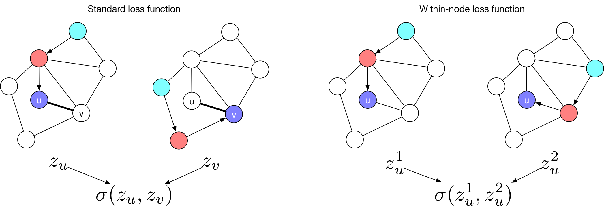
Figure 1. On the left an illustration of a standard unsupervised loss function, similar to (Hamilton et al., 2017b; Grover and Leskovec, 2016; Perozzi and Skiena, 2014). We term this $J_{neighbor}$ because it creates positive samples from neighbors in the graph: here, $u$ and $v$ are neighbors so $v$ is a positive example for $u$. On the right is the within-node loss function $J_{within}$ we propose in this paper. It uses as positive examples two samples from $u$’s own neighborhood. Nodes are colored by distance from a focal node, indicating that GNNs iteratively summarize further reaches of a focal node’s neighborhood.

Goal	Type	Features	Method
Role	Structural	$A,X_{s}$	GraphWAVE (Donnat et al., 2018), struc2vec (Ribeiro et al., 2017), role2vec (Ahmed et al., 2018), RolX (Henderson et al., 2012)
Role	Action	$A,X_{a}$	Role action embeddings (RAE, this paper)
Community	Structural	$A,X_{s}$	DeepWalk (Perozzi and Skiena, 2014), node2vec (Grover and Leskovec, 2016), unsupervised GraphSAGE (structural features) (Hamilton et al., 2017b)
Community	Action	$A,X_{a}$	unsupervised GraphSAGE (action features) (Hamilton et al., 2017b)

Table 1. Different node embedding types. Role embeddings place nodes with similar local neighborhoods close in embedding space. Community embeddings place nodes which tend to be linked close in embedding space.

2. Contributions

• We propose a within-node loss function which creates high-quality role embeddings, is compatible with scalable GNN architectures, and requires less graph information than an adjacency-based loss function

• We propose an unsupervised model architecture which learns quickly and is simpler than many alternatives

• We show that, for node classification tasks, focusing on action vectors of nodes leads to increased unsupervised performance over the common practice of concatenating action and structural features

• We introduce neighbor shuffling to quickly create training examples within batches

• We evaluate this framework (called RAE) in a variety of settings, finding good performance on both node and graph classification tasks

3. Setting and model

We have a graph $G=(V,E)$ which is treated as undirected. Each node in $G$ has a vector of attributes $X=(X_{s},X_{a})$, which can be divided into structural features $X_{s}$ and action features $X_{a}$. Structural features can include degree, clustering coefficient, and centrality measures. However, we assume only node degrees are readily available. Action features are characteristics of nodes, such as words in documents, chemical properties of molecules, or actions of people.

The goal is to find $d$-dimensional embeddings $z_{u}\in R^{d}$ for each node $u\in V$. Importantly, $z_{u}$ is required to be inductive, meaning embeddings of unseen nodes can be obtained.

We build on the GraphSAGE framework (Hamilton et al., 2017b) for this task. GraphSAGE takes a depth parameter $K$ and has two basic operations: combine and aggregate. At each depth $k\in\{1\dots K\}$, the representation from the previous layer $h_{u}^{k-1}$ is updated by sampling neighbors $\text{N}(u)$, and performing aggregate on neighbor features $\{h_{v}^{k-1}\;\forall v\in\text{N}(u)\}$. Then, this aggregated representation is combined with the existing representation to obtain

$$h_{u}^{k}=\textsc{combine}(h_{u}^{k-1},\textsc{aggregate}(\{h_{v}^{k-1}\;\forall v\in\text{N}(u)\}).$$

Note that usually $h_{u}^{0}=x_{u}$.

There are many possible choices for both combine and aggregate (Hamilton et al., 2017b; Xu et al., 2018; Chen et al., 2017). Common choices for combine are concatenation and mean, and common choices for aggregate are mean, max pool, summation, and LSTM. A fuller discussion of the strengths of different frameworks can be found in (Xu et al., 2018). The GraphSAGE framework is in some ways comparable to the Graph Convolutional Network (GCN) framework of (Kipf and Welling, 2016; Chen et al., 2018), although it is more scalable (Ying et al., 2018).

We propose a modification of GraphSAGE called RAE. There are several important differences from a standard GraphSAGE model. First, we ignore the combine operation entirely, and always include $u$ whenever the neighbor function $\text{N}(u)$ is used. For clarity, we write $\{u\}\cup\{x_{v}\>\forall\>v\in\text{N}(u)\}$. In combination with an elementwise mean aggregate function, this has the effect of blending together $u$’s embedding with its neighbors,.

Second, RAE uses a $\tanh$ activation function rather than the standard ReLU. Through experiments, we found dramatically increased unsupervised model performance. Algorithms 1 and 2 lay out the specifics of these choices.

Additionally, we make two practical decisions which improve performance. First, when generating two embeddings $z_{u}$ and $z_{v}$ which will be multiplied in a loss function, we generate $z_{u}$ and $z_{v}$ from two separate models, similarly to word2vec. Finally, GNNs have the powerful property of providing a distinct embedding at each aggregation level $\{1\dots K\}$. We specify $K=2$ below, and use both first and second step embeddings for prediction. This additional information improves model performance and is essentially free, since no additional model training is needed.

Algorithm 1 GNN architecture

Inputs: Graph $G=(V,E)$; action features $\{x_{u}^{a}\;\forall u\in V\}$; depth $K$; batch normalizers $B^{k}$; mean aggregators $\textsc{Agg}^{k}$; weight matrices $W^{k}$; dropout $D$; nonlinearity layer $\sigma^{k}=D(\text{tanh}(B^{k}(.)))$
Outputs: $d$-dimensional embeddings $z_{u}\;\forall u\in V$

1:procedure RAE

2:     $h_{u}^{0}\leftarrow x_{u}^{a}\>\forall\>u\in V$

3:     for $k\in\{1,\dots,K\}$ do

4:         for $u\in V$ do

5:              $h_{N(u)}^{k}\leftarrow\textsc{Agg}^{k}(u)$

6:              $h_{u}^{k}\leftarrow\sigma^{k}(W^{k}h_{N(u)}^{k})$               

7:     $z_{u}\leftarrow h_{u}^{K}\;\forall u\in V$

Algorithm 2 Mean aggregator

Inputs: Focal node $u$; graph $G=(V,E)$; arbitrary features $\{x_{u}\;\forall u\in V\}$; elementwise mean function $\textsc{Mean}(.)$; batch normalizer $B$; weight matrix $W$; neighborhood sampler $N(u)$; dropout $D$; nonlinearity layer $\sigma=D(\text{tanh}(B(.)))$
Outputs: $d$-dimensional neighbor summary for $u$, $h_{N(u)}\forall u\in V$

1:procedure MeanAggregator

2:     $h_{N(u)}\leftarrow\textsc{Mean}(\{u\}\cup\{x_{v}\>\forall\>v\in\textsc{N}(u)\})$

3:     $h_{N(u)}\leftarrow\sigma(W\cdot h_{u})$

4:     return $h_{N(u)}$

3.1. Within-node loss function for role embeddings

Consider two neighboring nodes, $(u,v)\in E$. The unsupervised loss function proposed by (Hamilton et al., 2017b) seeks to place $u$ and $v$ close in embedding space, by treating $z_{v}$ as a positive example for $z_{u}$,

(1) $$-J_{neighbor}=\sigma(z_{u}^{\text{T}}z_{v})+Q\,\mathbb{E}_{u_{n}\sim P(u)}[\sigma(-z_{u}^{\text{T}}z_{u_{n}})]$$

We refer to this as the “between node” or “neighbor” loss function. Here, $\sigma$ represents the logsigmoid transformation, $Q$ is the number of negative samples, and $P(u)$ samples a random node not adjacent to $u$. The intuition is close to that from word2vec (Mikolov et al., 2013) and associated methods applied to graphs such as DeepWalk (Perozzi and Skiena, 2014) and node2vec (Grover and Leskovec, 2016). Essentially, $J_{neighbor}$ treats $u$ as a collection of its neighbors $v$.

An alternate way to think about $u$’s position in embedding space is as a collection of substructures in its own local network neighborhood. Assume we take two samples from $u$’s local neighborhood $u_{1}$ and $u_{2}$ to create embeddings $z_{u_{1}}$ and $z_{u_{2}}$. We’d like these embeddings to be close in space, while the embedding of a walk from a random node random node $z_{w}$, $w\neq u$, should be more distant. The intuition here is closer to deep graph kernel techniques (Narayanan et al., 2017, 2016; Yanardag and Vishwanathan, 2015). Let $R(u)$ sample any $w\neq u$ at random. Then, we can create a within-node loss function

(2) $$-J_{within}=\sigma(z_{u_{1}}^{\text{T}}z_{u_{2}})+Q\,\mathbb{E}_{w\sim R(u)}[\sigma(-z_{u_{1}}^{\text{T}}z_{w})].$$

$J_{within}$ will place nodes close in embedding space when they themselves have similar local neighborhoods. For some graph structures, both $J_{neighbor}$ and $J_{within}$ will lead to similar embeddings, but this is not true in all cases. A simple example of divergence can be seen in Figure 2, where for depth $K=1$, $J_{neighbor}$ would consider $u$ and $v$ different since two-hop neighbors have different degrees. On the other hand, $J_{within}$ would consider $u$ and $v$ similar since the $K$-step neighborhoods are identical.

This highlights an important difference between $J_{neighbor}$ and $J_{within}$: $J_{within}$ requires relatively less graph information for each training pair since it relies on the $K$ step neighborhood of $u$ rather than the $K+1$ step neighborhood. This offers the possibility of faster training for large graphs, for instance by parallelizing individual neighborhoods. Below, we find that $J_{within}$ produces better role embeddings on ground-truth graphs when measured by silhouette score compared to $J_{neighbor}$.

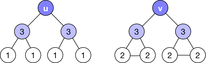
Figure 2. Local neighborhoods of nodes $u$ and $v$. Note that when considering node degree as a structural feature of nodes, the first order neighborhoods (light blue) are identical but the second order neighborhoods (white) are different. When choosing a depth of $K=1$, $J_{within}$ would consider $u$ and $v$ similar, while $J_{neighbor}$ would consider $u$ and $v$ different. This happens because $J_{neighbor}$ embeds nodes together when their neighbors (light blue) have similar $K$-hop neighborhoods. On the other hand, $J_{within}$ looks directly at the $K$-hop neighborhood of the focal nodes.

3.2. Neighbor shuffling

We expect embeddings based on two samples from $u$’s neighborhood to naturally be more similar than a sample from $u$ and from a random node $v$. If it is too easy for the model to distinguish samples from $u$ and negative samples from $v$, this could limit embedding quality.

To address this we introduce neighbor shuffling to create harder negative examples. This uses the the neighbors of some random node $v$ instead of $u$ to create negative examples. Practically, this means that we choose some $v\neq u$ in line 2 of Algorithm 2. Neighbor shuffling can be easily implemented within batches by permuting the within-batch adjacency list. This approach is similar to the idea of a corruption function in (Veličković et al., 2018) with an important distinction: we shuffle the neighbors rather than the features of $u$, which we found leads to better performance with RAE.

4. Role embedding performance on exemplar graphs

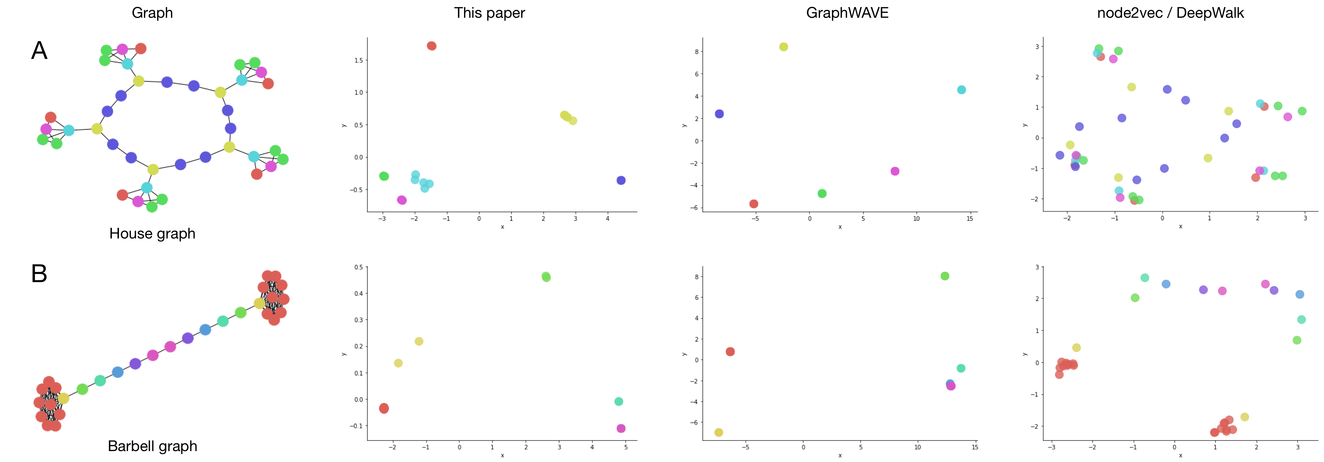
Figure 3. Performance of $J_{within}$ on two graphs with clear ground truth, the house and the barbell. Feature vectors used here are sorted degrees of neighbors. We take GraphWAVE (third column) as ground truth for this task. Note the intuitive difference between role embeddings (columns 2 and 3) and community-based embeddings (column 4).

Past work on structural role embeddings has studied the barbell and house graphs as visual tests of role embedding performance (Ribeiro et al., 2017; Donnat et al., 2018). Figure 3 displays our approach in comparison to two alternate methods. We use depth $K=2$, sorted vectors of neighbor degrees as node features, and train for 100 epochs. We sample 2 neighbors at depth $K=1$ and 4 neighbors at depth $K=2$.

We compare to GraphWAVE (Donnat et al., 2018) and node2vec/DeepWalk (Goyal and Ferrara, 2017; Perozzi and Skiena, 2014). GraphWAVE is a matrix factorization approach to structural role embeddings based on heat diffusion. Because of GraphWAVE’s strong performance for role embeddings, we consider it close to ground truth for this task. node2vec/DeepWalk provides a contrast between role embeddings and community-based embeddings. As expected, the structural role embeddings produced by our method display some variance when compared to GraphWAVE, but they reproduce the pattern of that strong baseline.

	$J_{within}$	$J_{neighbor}$
House graph	$91.2\pm 2.9\%$	$89.6\pm 4.2\%$
Barbell graph	$69.6\pm 8.1\%$	$69.5\pm 6.8\%$

Table 2. Silhouette scores and standard errors for ground-truth roles when using identical model setups with different loss functions, from 50 model runs. The differences are statistically significant for the house graph, using a two-sample two-sided t-test: $t=2.19,df=98,p<0.05$.

We compare the embeddings produced by $J_{within}$ and $J_{neighbor}$ in Table 2 on otherwise similar models using silhouette scores, finding that $J_{within}$ ranks higher, particularly for the house graph. This makes sense, since $J_{neighbor}$ represents nodes as combinations of their neighbors, leading to somewhat higher variance within roles. Both loss functions produce reasonable role embeddings in combination with structural features.

5. Experiments

We now turn to the performance of RAE on two types of tasks: node classification and graph classification.

Intuitively, good representations of a node’s neighborhood should allow classifying nodes well in an unsupervised setting. Further, the combination of embeddings for all nodes in a graph should provide distinct graph vectors suitable for graph classification. This treats a graph as a collection of roles. We note that these two tasks put RAE in comparison with two distinct lines of research: the first on node embeddings (Grover and Leskovec, 2016; Perozzi and Skiena, 2014; Hamilton et al., 2017b) and the second on graph kernels (Yanardag and Vishwanathan, 2015; Shervashidze and SHERVASHIDZE, 2011; Niepert et al., 2016; Verma and Zhang, 2018).

	Cora	Citeseer	Pubmed
Nodes	2,708	3,327	19,717
Edges	5,429	4,732	44,338
Features	1,433	3,703	500
Classes	7	6	3
Train/Val/Test	140/500/1,000	120/500/1,000	60/500/1,000

Table 3. Node classification datasets. The train/validation/test sets splits are set by (Kipf and Welling, 2016).

Method	MUTAG	IMDB-B	REDDIT-B	IMDB-M	REDDIT-M5K	REDDIT-M12K
Baselines
DGK (Yanardag and Vishwanathan, 2015)	87.4	67.0	78.0	44.6	41.3	32.2
Patchy-san (Niepert et al., 2016)	92.6	71.0	86.3	45.2	49.1	41.3
GIN (Xu et al., 2018)	90.0	75.1	92.4	52.3	57.5	-
RAE (this paper)
Untrained	$88.1\pm 0.9\%$	$72.7\pm 0.9\%$	$81.6\pm 1.4\%$	$50.6\pm 0.5\%$	$54.3\pm 1.4\%$	$43.5\pm 1.8\%$

Table 4. Results for graph classification tasks with standard deviations from 20 runs. Note that GIN (Xu et al., 2018) provides an upper bound for expressiveness with a GNN framework.

5.1. Model setup

Information	Method	d	K	Cora	Citeseer	Pubmed
Unsupervised baselines
$X_{a}$	L2 regression	$|X_{a}|$	0	58.9	60.4	72.9
$A$	DeepWalk (Kipf and Welling, 2016)	128	5	67.2	43.2	65.3
$A,X_{a}$	DeepWalk + $X_{a}$ (Hamilton et al., 2017b)	128 + $|X_{a}|$	5	70.7	51.4	74.3
$A,X_{a}$	DGI (Veličković et al., 2018)	512 (256 on Pubmed)	3	82.3	71.8	76.8
$A,X_{a}$	EP-B (Garcia Duran and Niepert, 2017)	128	1	78.1	71.0	80.0
RAE (this paper)
$A,X_{a}$	Untrained	256	2	$57.0\pm 2.7\%$	$46.0\pm 3.4\%$	$65.7\pm 2.3\%$
$A,X_{a}$	$J_{within}$ (only shuffling)	256	2	$77.5\pm 1.1\%$	$67.2\pm 1.0\%$	$76.9\pm 1.8\%$
$A,X_{a}$	$J_{within}$	256	2	$78.0\pm 0.9\%$	$67.6\pm 1.1\%$	$77.0\pm 1.8\%$
$A,X_{a}$	$J_{neighbor}$	256	2	$79.3\pm 1.2\%$	$68.1\pm 1.3\%$	$\underline{79.5}\pm 0.7\%$
$A,X_{a}$	concat($J_{within},J_{neighbor}$)	256 + 256	2	$\underline{80.2}\pm 0.9\%$	$68.0\pm 1.2\%$	$78.7\pm 0.9\%$
Semi-supervised models
$A,X_{a},Y$	Planetoid (Yang et al., 2016)	-	-	75.7	64.7	77.2
$A,X_{a},X_{s},Y$	GraphSAGE (Chen et al., 2017)	32	2	82.0	70.8	79.0
$A,X_{a},Y$	GCN (Kipf and Welling, 2016)	16	2	81.5	70.3	79.0
$A,X_{a},Y$	GAT (Velic?kovic et al., 2018)	64	3	83.0	72.5	79.0
$A,X_{a},Y$	FastGCN-transductive (Chen et al., 2018)	16	2	81.8	-	77.6

Table 5. Accuracy and mean standard errors of various methods on three standard node classification tasks. The left column indicates which information is available to the algorithm: $A$ the adjacency matrix, $X_{s}$ structural features, $X_{a}$ action features, $Y$ the outcome of interest. $d$ is either the embedding dimension in the unsupervised case, or the dimension of the last hidden layer in the supervised case. $K$ is the maximum depth in the network that the model has access to. The first block presents unsupervised baselines, the second block presents results from our modeling architecture, the third block presents semi-supervised models. The best unsupervised model is bolded, and the second best is underlined.

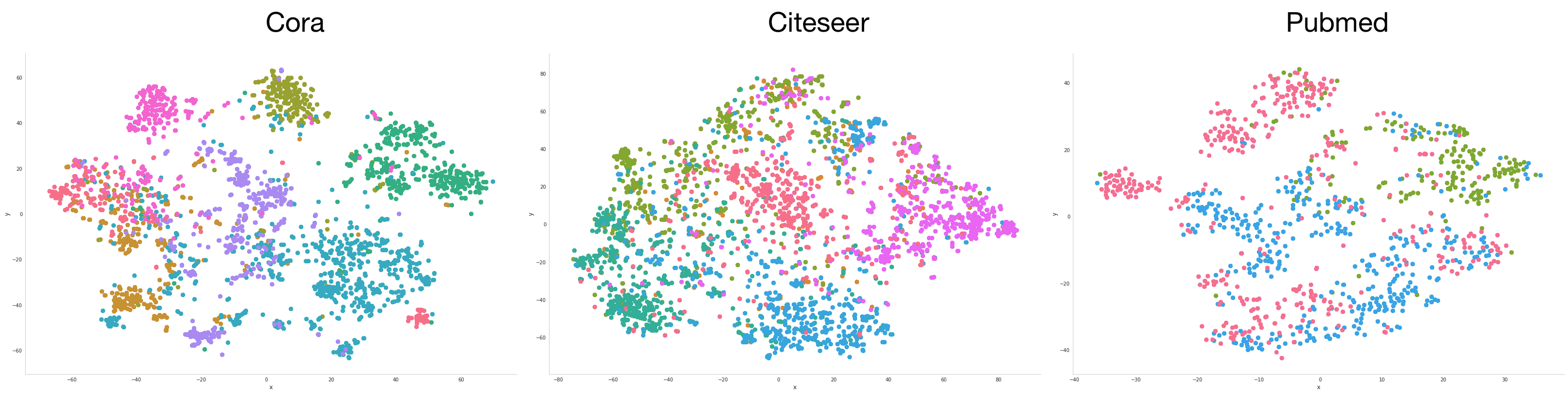
Figure 4. Visualization of embeddings on three citation graphs using RAE with $J_{within}$, reduced to two dimensions using TSNE. For Cora and Citeseer, we used the entire dataset, while we visualize the test set for Pubmed. Clusters are quite distinct in all cases. On Cora, this model achieves a silhouette score of 0.166.

We describe model architecture in Algorithms 1 and 2. We choose depth $K=2$, and sample sample 10 neighbors at depth $K=1$ and 25 neighbors at depth $K=2$, for a total receptive field of 261 nodes (ego + 10 at depth 1 + 250 at depth 2). We use a dropout rate of 0.6, a constant learning rate of 0.01, and a batch size of 256. Unless noted, models are trained for 200 epochs, where each epoch considers a single batch. This means that even though graph sizes vary, a constant 51,200 training examples are used in all cases. We choose an output layer dimension of $d_{K=1}=64$ and a hidden layer representation of $d_{K=2}=192$. The embedding dimension is therefore $d=256$, since it’s a concatenation of the representation from $K=1$ and $K=2$.

The model is trained with 5 positive examples and 20 negative examples, using $J_{within}$ or $J_{neighbor}$ directly with no margin. When using $J_{within}$, half of the negative examples are generated via neighbor shuffling and half are generated randomly from $R(u)$. For $J_{neighbor}$, all negative examples are generated from non-neighbors with $P(u)$. Models are trained with Adam (Kingma and Ba, 2014) and initialized with Xavier uniform weights (Glorot and Bengio, 2010).

In the case of sparse input vectors representing text in citation networks, no preprocessing is performed. This means directly inputting high-dimensional (500 to 3703) sparse vectors into the model. Following common practice, we use embeddings in an L2-penalized logistic regression model. In the multiclass case, a one-vs-rest classifier is used. To obtain an accurate picture of both performance and variance, we report results from 20 runs, providing mean performance and standard deviation of the mean.

Our choices of $d=256$, $K=2$ and a receptive field of 261 are equivalent or conservative compared to prior research on GNNs. For instance, (Veličković et al., 2018) use $d=512$ and $K=3$, and (Hamilton et al., 2017a) use $d=256$ and $K=2$. Since the output dimension for RAE is set to $d_{K=1}=64$, we use many fewer parameters than a GraphSAGE-style model which has both hidden and output dimensions of 256.

5.2. Graph classification results

We choose six standard datasets studied in the graph classification literature (full dataset descriptions can be found in (Yanardag and Vishwanathan, 2015)), with results presented in Table 4. Most of these datasets do not have features beyond those from the graph itself. In these cases, we label each node with the sorted degrees of its neighbors, capped at 30. When a node has more than 30 neighbors, we sample randomly; when it has fewer, we pad with zeros. For MUTAG, IMDB-B, and REDDIT-B only sample 4 neighbors are sampled at depth 1 and 4 at depth 2, for a total receptive field of 21. For the rest of the graphs we use the parameters described above. We observed that training did not substantially improve performance, so these models are untrained. They therefore indicate the raw expressive power of the model. A discussion of different GNN architectures and theoretical performance guarantees can be found in (Xu et al., 2018).

Since each node has a $d$-dimensional vector, we need to choose a “readout” function to produce graph vectors from node vectors. We choose a simple summation to represent the embedding for graph $G_{i}$: $z_{G_{i}}=\sum_{u\in G_{i}}z_{u}$. Graph vectors $z_{G_{i}}$ are then employed in a one-vs-rest classification problem using 10-fold cross validation. In the binary classification case, we use the test folds to select the probability cutoff which maximizes test fold accuracy.

RAE outperforms two strong baselines on many of the graph classification tasks: deep graph kernels (Yanardag and Vishwanathan, 2015) and Patchy-san (Niepert et al., 2016). We also include graph isomorphism networks (GIN) (Xu et al., 2018) to give an idea of the upper bound for model expressiveness if we were to use one-hot encodings for features, a summation aggregator, training, and a larger $K$. The simple mean framework we use performs quite well.

5.3. Node classification results

We choose three standard datasets which provide both graphs and rich features: Cora, Citeseer, and Pubmed. Dataset details can be found in Table 3. These are citation datasets where each node is a paper and each link is a citation. Each paper is annotated with a sparse vector representing the words used in the paper. We follow the procedure described in (Kipf and Welling, 2016) for these datasets: 20 nodes are selected as training examples from each class, with 1000 nodes selected as test nodes and 500 as validation. We use the same splits used by Kipf and Welling. We optimized hyperparameters on the validation set given by Kipf and Welling, but do not make use of validation set on the fly to determine early stopping. Hyperparameters were tuned on the Cora dataset and then applied these settings directly to Citeseer and Pubmed.

Table 5 presents results of RAE compared to a variety of other unsupervised and semi-supervised baselines. The most direct comparison is with other unsupervised methods. All versions of RAE outperform DeepWalk-based methods (including node features directly). Moving to two more difficult baselines, RAE outperforms Deep Graph Infomax (DGI) (Veličković et al., 2018) on Pubmed and EP-B (Garcia Duran and Niepert, 2017) on Cora. DGI has access to depth 3 rather than the depth 2 used in our model, making the performance of RAE impressive. EP-B is an efficient method which does a single aggregation step, but also comes with a margin hyperparameter which must be tuned, and samples all neighbors of a focal node as opposed to the fixed number used here.

Surprisingly, RAE with $J_{neighbor}$ outperforms the supervised models on Pubmed, and scores the second highest overall. These results indicate that the modeling framework proposed here provides strong performance on these standard tasks despite model simplicity. $J_{within}$ using only neighbor shuffling—the most scalable parameterization of RAE—performs comparably to DGI on Pubmed and only a shade below EP-B on Cora. The most puzzling part of these results is the weak performance on Citeseer, which could be related to the larger input dimension (3703). Regularization may help in this setting, but was not employed since it did not prove effective when developing the model on the Cora validation set.

The embeddings presented here do not incorporate structural features (e.g. degree, neighbor degrees, motif counts) in the input vector (Hamilton et al., 2017b; Henderson et al., 2012; Ahmed et al., 2018). We therefore refer to them as action embeddings. We consistently found that including even node degree in the feature vector reduced performance. This implies that unsupervised GNNs are not adept at preserving both structural and action features without additional modeling work. Structural features easily overwhelm sparse action features.

The combination of $J_{within}$ and $J_{between}$ provides the strongest performance on Cora, but not on the other two datasets. While this may seem surprising, it is potentially related to the small size of the training set (20 nodes per class). As a final note, we have considered only transductive embeddings here, but RAE can be applied inductively as well.

6. Conclusion

We have presented RAE, a scalable methodology for learning role embeddings, and introduced the concept of role action embeddings. This creates a useful distinction in the type of information which may be incorporated into node embeddings, in addition to providing strong performance on several standard tasks.

We note that the performance of action feature embeddings is related to the type of task under consideration: when classifying papers into topic categories, it makes sense that paper text is important. However, without knowledge of how embeddings will be used beforehand, this distinction creates a challenge for researchers. A simple response is to train separate models for structural and action features. A direction for future work is to combine these two types of features with novel model architectures. In addition to the intuitive usefulness of role action embeddings, the modeling choices we have made are likely to be useful in other settings as well.

7. Acknowledgements

Thanks to Nima Noorshams, Katerina Marazopoulou, Lada Adamic, Saurabh Verma, Alex Dow, Shaili Jain, and Alex Pesyakhovich for discussions and suggestions.

References

- (1)
- Ahmed et al. (2018) Nesreen K. Ahmed, Ryan Rossi, John Boaz Lee, Xiangnan Kong, Theodore L. Willke, Rong Zhou, and Hoda Eldardiry. 2018. Learning Role-based Graph Embeddings. arXiv:1802.02896 [cs, stat] (Feb. 2018). http://arxiv.org/abs/1802.02896 arXiv: 1802.02896.
- Burt (1978) Ronald S. Burt. 1978. Cohesion Versus Structural Equivalence as a Basis for Network Subgroups. Sociol. Methods Res. 7, 2 (1978), 189–212.
- Chen et al. (2018) Jie Chen, Tengfei Ma, and Cao Xiao. 2018. FastGCN: Fast Learning with Graph Convolutional Networks via Importance Sampling. arXiv:1801.10247 [cs] (Jan. 2018). http://arxiv.org/abs/1801.10247 arXiv: 1801.10247.
- Chen et al. (2017) Jianfei Chen, Jun Zhu, and Le Song. 2017. Stochastic Training of Graph Convolutional Networks with Variance Reduction. arXiv:1710.10568 [cs, stat] (Oct. 2017). http://arxiv.org/abs/1710.10568 arXiv: 1710.10568.
- Donnat et al. (2018) Claire Donnat, Marinka Zitnik, David Hallac, and Jure Leskovec. 2018. Learning Structural Node Embeddings via Diffusion Wavelets. (2018), 10.
- Garcia Duran and Niepert (2017) Alberto Garcia Duran and Mathias Niepert. 2017. Learning Graph Representations with Embedding Propagation. In Advances in Neural Information Processing Systems 30, I. Guyon, U. V. Luxburg, S. Bengio, H. Wallach, R. Fergus, S. Vishwanathan, and R. Garnett (Eds.). Curran Associates, Inc., 5119–5130. http://papers.nips.cc/paper/7097-learning-graph-representations-with-embedding-propagation.pdf
- Glorot and Bengio (2010) Xavier Glorot and Yoshua Bengio. 2010. Understanding the difficulty of training deep feedforward neural networks. (2010), 8.
- Goyal and Ferrara (2017) Palash Goyal and Emilio Ferrara. 2017. Graph Embedding Techniques, Applications, and Performance: A Survey. arXiv:1705.02801 [physics] (May 2017). http://arxiv.org/abs/1705.02801 arXiv: 1705.02801.
- Grover and Leskovec (2016) Aditya Grover and Jure Leskovec. 2016. node2vec: Scalable Feature Learning for Networks. ACM Press, 855–864. https://doi.org/10.1145/2939672.2939754
- Hamilton et al. (2017a) Will Hamilton, Zhitao Ying, and Jure Leskovec. 2017a. Inductive representation learning on large graphs. In Advances in Neural Information Processing Systems. 1025–1035.
- Hamilton et al. (2017b) William L. Hamilton, Rex Ying, and Jure Leskovec. 2017b. Representation Learning on Graphs: Methods and Applications. arXiv:1709.05584 [cs] (Sept. 2017). http://arxiv.org/abs/1709.05584 arXiv: 1709.05584.
- Henderson et al. (2012) Keith Henderson, Brian Gallagher, Tina Eliassi-Rad, Hanghang Tong, Sugato Basu, Leman Akoglu, Danai Koutra, Christos Faloutsos, and Lei Li. 2012. RolX: structural role extraction & mining in large graphs. ACM Press, 1231. https://doi.org/10.1145/2339530.2339723
- Kingma and Ba (2014) Diederik P. Kingma and Jimmy Ba. 2014. Adam: A Method for Stochastic Optimization. arXiv:1412.6980 [cs] (Dec. 2014). http://arxiv.org/abs/1412.6980 arXiv: 1412.6980.
- Kipf and Welling (2016) Thomas N. Kipf and Max Welling. 2016. Semi-Supervised Classification with Graph Convolutional Networks. arXiv:1609.02907 [cs, stat] (Sept. 2016). http://arxiv.org/abs/1609.02907 arXiv: 1609.02907.
- Mikolov et al. (2013) Tomas Mikolov, Kai Chen, Greg Corrado, and Jeffrey Dean. 2013. Efficient Estimation of Word Representations in Vector Space. arXiv:1301.3781 [cs] (Jan. 2013). http://arxiv.org/abs/1301.3781 arXiv: 1301.3781.
- Narayanan et al. (2016) Annamalai Narayanan, Mahinthan Chandramohan, Lihui Chen, Yang Liu, and Santhoshkumar Saminathan. 2016. subgraph2vec: Learning Distributed Representations of Rooted Sub-graphs from Large Graphs. arXiv:1606.08928 [cs] (June 2016). http://arxiv.org/abs/1606.08928 arXiv: 1606.08928.
- Narayanan et al. (2017) Annamalai Narayanan, Mahinthan Chandramohan, Rajasekar Venkatesan, Lihui Chen, Yang Liu, and Shantanu Jaiswal. 2017. graph2vec: Learning Distributed Representations of Graphs. arXiv:1707.05005 [cs] (July 2017). http://arxiv.org/abs/1707.05005 arXiv: 1707.05005.
- Niepert et al. (2016) Mathias Niepert, Mohamed Ahmed, and Konstantin Kutzkov. 2016. Learning Convolutional Neural Networks for Graphs. (2016), 10.
- Perozzi and Skiena (2014) Bryan Perozzi and Steven Skiena. 2014. DeepWalk : Online Learning of Social Representations. Sigkdd (2014), 701–710. https://doi.org/10.1145/2623330.2623732
- Ribeiro et al. (2017) Leonardo F. R. Ribeiro, Pedro H. P. Saverese, and Daniel R. Figueiredo. 2017. struc2vec: Learning Node Representations from Structural Identity. arXiv:1704.03165 [cs, stat] (2017), 385–394. https://doi.org/10.1145/3097983.3098061 arXiv: 1704.03165.
- Shervashidze and SHERVASHIDZE (2011) Nino Shervashidze and NINO SHERVASHIDZE. 2011. Weisfeiler-Lehman Graph Kernels. (2011), 23.
- Velic?kovic et al. (2018) Petar Velic?kovic, Guillem Cucurull, Arantxa Casanova, Adriana Romero, Pietro Lio, and Yoshua Bengio. 2018. GRAPH ATTENTION NETWORKS. (2018), 12.
- Veličković et al. (2018) Petar Veličković, William Fedus, William L. Hamilton, Pietro Liò, Yoshua Bengio, and R. Devon Hjelm. 2018. Deep Graph Infomax. arXiv:1809.10341 [cs, math, stat] (Sept. 2018). http://arxiv.org/abs/1809.10341 arXiv: 1809.10341.
- Verma and Zhang (2018) Saurabh Verma and Zhi-Li Zhang. 2018. Graph Capsule Convolutional Neural Networks. arXiv:1805.08090 [cs, stat] (May 2018). http://arxiv.org/abs/1805.08090 arXiv: 1805.08090.
- White et al. (1976) Harrison C. White, Scott A. Boorman, and Ronald L. Breiger. 1976. Social Structure from Multiple Networks. I. Blockmodels of Roles and Positions. Amer. J. Sociology 81, 4 (1976), 730–780. http://www.jstor.org/stable/2777596
- Xu et al. (2018) Keyulu Xu, Weihua Hu, Jure Leskovec, and Stefanie Jegelka. 2018. HOW POWERFUL ARE GRAPH NEURAL NETWORKS? (2018), 15.
- Yanardag and Vishwanathan (2015) Pinar Yanardag and S.V.N. Vishwanathan. 2015. Deep Graph Kernels. ACM Press, 1365–1374. https://doi.org/10.1145/2783258.2783417
- Yang et al. (2016) Zhilin Yang, William W Cohen, and Ruslan Salakhutdinov. 2016. Revisiting Semi-Supervised Learning with Graph Embeddings. (2016), 9.
- Ying et al. (2018) Rex Ying, Ruining He, Kaifeng Chen, Pong Eksombatchai, William L. Hamilton, and Jure Leskovec. 2018. Graph Convolutional Neural Networks for Web-Scale Recommender Systems. arXiv:1806.01973 [cs, stat] (June 2018). https://doi.org/10.1145/3219819.3219890 arXiv: 1806.01973.