Synthetic Lung Nodule 3D Image Generation Using Autoencoders

Abstract

One of the challenges of using machine learning techniques with medical data is the frequent dearth of source image data on which to train. A representative example is automated lung cancer diagnosis, where nodule images need to be classified as suspicious or benign. In this work we propose an automatic synthetic lung nodule image generator. Our 3D shape generator is designed to augment the variety of 3D images. Our proposed system takes root in autoencoder techniques, and we provide extensive experimental characterization that demonstrates its ability to produce quality synthetic images.

I Introduction

Year after year, lung cancer is consistently one of the leading causes of cancer deaths in the world [1]. Computer aided diagnosis, where a software tool proposes a diagnosis after analyzing the patient’s medical imaging results, is a promising direction: from an input low-resolution 3D CT scan, image analysis techniques can be used to classify nodules in the lung scan as benign or potentially cancerous. But such systems require large amounts of labeled 3D training images to ensure the classifiers are adequately trained with sufficient generality. Especially when new technologies are developed, cancerous lung nodule detection still suffers from a dearth of training images which hampers the ability to effectively improve and automate the analysis of CT scans for cancer risks [2]. In this work, we propose to address this problem by automatically generating synthetic 3D images of lung nodules, to augment the training dataset of such systems with meaningful (yet computer-generated) images [3].

Features of lung nodules computed from 3D images can be used as inputs to a nodule classification algorithm. Features such as volume, degree of compactness, surface area to volume ratio, etc. have been useful in classifying lung nodules [4]. 2D lung nodule images that are realistic enough to be classified by radiologists as actual CT scan images have been created using generative adversarial networks (GANs) [5]. In our work, we aim to generate 3D lung nodule images which match the feature statistics of actual nodules as determined by an analysis program. We propose a new system inspired from autoencoders, and extensively evaluate its generative capabilities. Precisely, we present in detail LuNG: a synthetic lung nodule generator, which is a neural network trained to generate new examples of 3D shapes that fit within a broad learned category [3].

To improve automatic classification in cases where input images are difficult to acquire, our work aims to create realistic synthetic images given a set of seed images. For example, the Adaptive Lung Nodule Screening Benchmark (ALNSB) from the NSF Center for Domain-Specific Computing [6] uses a flow that leverages compressive sensing to reconstruct images from low-dose CT scans. Compared to compressive sensing, filtered backprojection is a technique which has more samples readily available (such as LIDC/IDRI [7]), but filtered backprojection has slightly different images that are not appropriate for training ALNSB.

For evaluation, we integrated our work with ALNSB [8] that automatically processes a low-dose 3D CT scan, reconstructs a higher-resolution image, isolates all nodules in the 3D image, computes features on them and classifies each nodule as benign or suspicious. We train LuNG using original patient data, and use it to generate synthetic nodules ALNSB can process. We create a network which optimizes 4 metrics: (1) increase the percentage of generated images accepted by the nodule analyzer; (2) increase the variation of the generated output images relative to the limited seed images; (3) decrease the difference of the means for computed features of the output images relative to seed images; and (4) decrease the autoencoder reproduction error for the seed images.

We make the following contributions. First, we present LuNG, a new automated system for the generation of synthetic 3D images that span the feature space of the input training images. It uses novel metrics for the numerical evaluation of 3D image generation aligned with qualitative goals related to lung nodule generation. Second, we conduct an extensive evaluation of this system to generate 3D lung nodule images, and its use within an existing computer-aided diagnosis benchmark application including iterative training techniques to further refine the quality of the image generator.

The rest of the paper is organized as follows. Section II briefly motivates our work and design choices. Section III describes the LuNG system. Extensive experimental evaluation is presented in Section IV. Related work is discussed in Section V before concluding.

II Motivation

To improve early detection and reduce lung cancer mortality rates, the research community needs to improve lung nodule detection even given low resolution images and a small number of sample images for training. The images have low resolution because low radiation dosages allow for screening to be performed more frequently to aid in early detection, but the low radiation dosage limits the spatial resolution of the image. The number of training samples is small due in part to patient privacy concerns but is also related to the rate at which new medical technology is being created which generates a need for new training data on the new technology. Our primary goal is to create 3D voxel images that are within the broad class of legal nodule shapes that may be generated from a CT scan.

With the goal of creating improved images for training, we evaluate nodules generated from our trained network using the same software that analyzes the CT scans for lung nodules. Given the availability of ’accepted’ new nodules, we test augmenting the training set with these nodules to improve generality of the network. The feedback process we explore includes a nodule reconnection step (to insure final nodules are fully connected in 3D space) followed by a pass through the analyzer which will prune the generated set to keep 3D nodule feature means close to the original limited training set. The need to avoid overfitting the network for a small set of example images, as well as learning a 3D image category by examples, guided many of the network architecture decisions presented below.

While one goal of our work is to demonstrate the possibility to create a family of images which have computed characteristics (e.g., elongation, volume) that fit within a particular distribution range; another goal is to generate novel images that are similar to an observed input nodule image. Hence, in addition to creating a generator network, we shall create a feature network that can receive a seed image as input and produce as outputs values for the generator that reproduce the seed image. The goal of generating images related to a given input image motivates our inclusion of the reconnection algorithm. Other generative networks will prune illegal outputs as part of their use model [9], but we wanted to provide more guarantee of valid images when exploring the feature space near a given sample input. The goal of finding latent feature values for existing images leads naturally to an autoencoder architecture for our neural network.

Generative adversarial networks (GANs) [10] and variational autoencoders (VAEs) [11] are two sensible approaches to generate synthetic images from a training set and could intuitively be applied to our problem. However, traditional GANs do not provide a direct mapping from source images into the generator input feature space [12], which limits the ability to generate images similar to a specific input sample or require possibly heavy filtering of “invalid” images produced by the network. In contrast, using an autoencoder-based approach as we develop below allows to better explore the feature space near the seed images. A system that combines the training of an autoencoder with a discriminator network such as GRASS [10] would allow some of the benefits of GAN to be explored relative to our goals. However, our primary goal is not to create images that match the distribution of a training set as determined by a loss function. As we show in section III-D, our goal can be summarized as creating novel images that are within a category acceptable to an automated nodule analyzer. As such, we strive to generate images that are not identical to the source images but fit within a broad category learned by the network.

A similar line of reasoning can be applied to VAEs relative to our goals. Variational autoencoders map the distribution of the input to a generator network to allow for exploration of images within a distributional space. In our work, we tightly constrain our latent feature space so that our training images map into the space but the space itself may not match the seed distribution exactly to aid in the production of novel images. Like GANs, there are ways to incorporate VAEs into our framework, and to some extent our proposed approach is a form of variational autoencoder, although with clear differences in both the training and evaluation loop, as developed below. Our work demonstrates one sensible approach for a full end-to-end system to create synthetic 3D images that can effectively cover the feature space of 3D lung nodules reconstructed via compressive sensing.

III The LuNG System

The LuNG system is based on a neural network trained to produce realistic 3D lung nodules from a small set of seed examples to help improve automated cancer screening. To provide a broader range of legal images, guided training is used in which each nodule is modified to create 15 additional training samples. We call the initial nodule set, of which we were provided 51 samples, the ’seed’ nodules. The ’base’ nodules include 15 modified samples per seed nodule for a total of 816 samples. The base nodules are used to train an autoencoder neural network with 3 latent feature neurons in the bottleneck layer. The output of the autoencoder goes through a reconnection algorithm to increase the likelihood that viable fully connected nodules are being generated. A nodule analyzer program then extracts relevant 3D features from the nodules and prunes away nodules outside the range of interesting feature values. We use the ALNSB [8] nodule analyzer and classifier code for LuNG. The accepted nodules are the final output of LuNG for use in classifier training or medical evaluation. Given this set of generated images which have been accepted by the analyzer, we explore adding them to the autoencoder training set to improve the generality of the generator. We explore having a single generator network or 2 networks that exchange training samples.

III-A Input images

The input dataset comes from the Automatic Lung Screening Benchmark (ALNSB) [8], produced by the NSF Center for Domain-Specific Computing [6]. This pipeline, shown in figure 1, is targeting the automatic reconstruction of 3D CT scans obtained with reduced (low-dose) radiation, i.e., reducing the number of samples taken by the machine. Compressive sensing is used to reconstruct the initial 3D image of a lung, including all artifacts such as airways, etc. A series of image processing steps are performed to isolate all nodules that could lie along the tissue. Then, each of the 3D candidate nodules is analyzed to obtain a series of domain-specific metrics, such as elongation, volume, surface area, etc. An initial filtering is done based on static criteria (e.g., volume greater than $4\text{mm}^{3}$) to prune nodules that are not suspicious for potential cancerous origin. Eventually, the remaining nodules are fed to a trained SVM-based classifier, which classifies the nodules as potentially cancerous or not. The end goal of this process is to trigger a high-resolution scan for only the regions containing suspicious nodules, while the patient is still on the table.

This processing pipeline is extremely specific regarding both the method used to obtain and reconstruct the image, via compressive sensing, and the filtering imposed by radiologists regarding the nodule metrics and their values about potentially cancerous nodules. In this paper, we operate with a single-patient data as input, that is, a single 3D lung scan. About 2000 nodules are extracted from this single scan, out of which only 51 are true candidates for the classifier. Our objective is to create a family of nodules that are also acceptable inputs to the classifier (i.e., which have not been dismissed early on based on simple thresholds on the nodule metrics), starting from these 51 images. We believe this represents a worst-case scenario where the lack of input images is not even sufficient to adequately train a simple classifier and is therefore a sensible scenario to demonstrate our approach to generating images within a specific acceptable feature distribution.

These 51 seed images represent the general nodule shape that we wish to generate new nodules from. Based on the largest of these 51 images, we set our input image size to 25$\times$28$\times$28mm, which also aligns with other nodule studies [4]. The voxel size from the image processing pipeline is 1.25$\times$0.7$\times$0.7mm, so our input nodules are 20$\times$40$\times$40 voxels. This results in an input to the autoencoder with 32,000 voxel values which can range from 0 to 1.

Figure 1: Medical image processing pipeline [6]

Figure 2: Six of the 51 seed nodules showing the middle 8 out of 20 2D slices

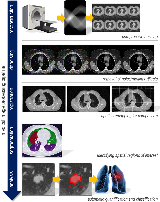
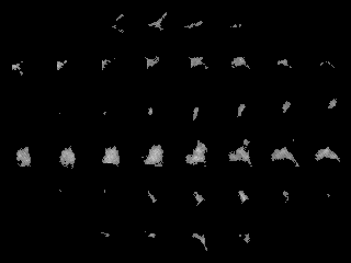
Figure 2 shows 6 of the 51 seed images from the CT scan. Each of the images is centered in the 20$\times$40$\times$40 training size. One of our nodules was slightly too wide and 21 out of 1290 total voxels were clipped; all other nodules fit within the training size. From an original set of 51 images, 816 are generated: 8 copies of each nodule are the 8 possible reflections in X,Y, and Z of the original; and 8 copies are the X,Y, and Z reflections of the original shifted by 0.5 pixels in X and Y. The reflections are still representative of legal nodule shapes to the analyzer, so it improves the generality of the autoencoder to have them included. The 0.5-pixel shift also aids generalization of the network by training it to tolerate fuzzy edges and less precise pixel values. We do not do any resizing of the images as we found through early testing that utilizing the full voxel data resulted in better generated images than resizing the input and output of the autoencoder.

Our initial 51 seed images include 2 that are classified as suspicious nodules. These 2 seed images become 32 images in our base training set, but still provide us with a limited example of potentially cancerous nodules. A primary goal of the LuNG system is to create a wider variety of images for use in classification based on learning a nodule feature space from the full set of 51 input images.

III-B Autoencoder network

Figure 3 shows the autoencoder structure as well as the feature and generator networks that are derived from it. All internal layers use tanh for non-linearity, which results in a range of -1 to 1 for our latent feature space. The final layer of the autoencoder uses a sigmoid function to keep the output within the 0 to 1 range that we are targeting for voxel values.

We experimented with various sizes for our network and various methods of providing image feedback from the analyzer with results shown in section IV. The network shown in figure 3 had the best overall $Score$.

Figure 3: Autoencoder and derived feature/generator networks for nodules

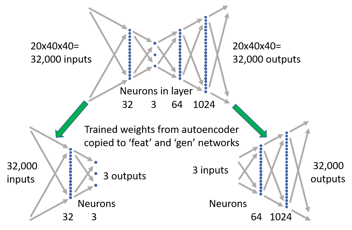
Our autoencoder is trained initially with the 816 images in our base set. We use Adam [13] for stochastic optimization to minimize the mean squared error of the generated 32,000 voxel 3D images. After creating a well-trained autoencoder, the network can be split into feature and generator networks. The feature network can be used to map actual nodules into a latent feature space so that novel images similar to the actual input nodule can be created using the generator network. If stepping is done between the latent feature values of nodule suspected as cancerous and another suspected to be non-cancerous, a skilled neurologist could identify the shape at which the original suspicious nodule would not be considered suspicious to help train and improve an automated classifier. The generator network can also be used to generate fully random images for improving a classifier. For our random generation experiments we use uniform values from -1 to 1 as inputs for the 3 latent feature dimensions. We explore the reasons and benefits of this random distribution in section IV-C.

The autoencoder structure which yielded the best results is not symmetric in that there are fewer layers before the bottleneck layer than after. Like the seminal work by Hinton and Salakhutdinov [14], we explored various autoencoder sizes for our problem, but we added in an exploration of non-symmetric autoencoders. We found during hyperparameter testing that a 2-layer feature network (encoder) performed better than a 1-layer or 3-layer network. We suspect that a single layer for the feature network was not optimal due to limiting the feature encoding of the input images to linear combinations of principle components [15]. We suspect that 3 layers for our feature network was less optimal than 2 layers due to overfitting the model to our limited training set. Given our goal of generating novel nodule shapes, overfitting is a particular concern and we address this using a network scoring metric discussed in section III-D.

III-C Reconnection algorithm

The autoencoder was trained on single component nodules in that all the ’on’ voxels for the nodule were connected in a single 3D shape. The variation produced by trained generator networks did not always result in a single component, and it is common for generative networks that have a technical constraint to discard output which fails to meet the requirements [9]. However, for the use case of exploring the feature space near a known image, we chose to add a reconnection algorithm to our output nodules to minimize illegal outputs. This algorithm insures that for any input to the generative network, a fully-connected nodule is generated.

When the generator network creates an image, a single fully-connected component is usually generated and the reconnection algorithm does not need to be invoked. In the case where multiple components are detected, the algorithm will search through all empty voxels and set a small number of them to connect the components into a single nodule.

III-D Metrics for nodule analyzer acceptance and results scoring

The nodule analyzer and classifier computes twelve 3D feature values for each nodule (features such as 3D volume, surface-to-volume ratio, and other data useful for classification). Our statistical approach to this data is related to Mahalanobis distances [16], hence we compute the mean and standard deviations on these 12 features for the 51 seed nodules. Random nodules from the generator are fed into the classifier code and accepted to produce similar feature values. This accepted set of images is the most useful image set for further analysis or use in classifier training.

Metrics for analyzer acceptance of the images

Using the mean and standard deviation values we create a distance metric $d$ based on concepts similar to the Mahalanobis distance. Given $S$ is the set of 51 seed nodules and $i$ is the index for one of 12 features, $\mu_{Si}$ is the mean value of feature $i$ and $\sigma_{Si}$ is the standard deviation. Given Y is the set of output nodules from LuNG, the running mean for feature $i$ of the nodules being analyzed is $\bar{Y_{i}}$. Given feature $i$ of a nodule $y$ is $y_{i}$ then if either (${y_{i}\geq\mu_{Si}}$ and $\bar{Y_{i}}\leq\mu_{Si}$) or ($y_{i}\leq\mu_{Si}$ and $\bar{Y_{i}}\geq\mu_{Si}$), then the nodule is accepted as it helps $\bar{Y_{i}}$ trend towards $\mu_{Si}$. In cases where the nodule’s $y_{i}$ moves $\bar{Y_{i}}$ away from $\mu_{Si}$, we compute a weighted distance $d$ from $\mu_{Si}$ in multiples of ${\sigma_{Si}}$ using:

$$d=|\frac{y_{i}+3*\bar{Y_{i}}-4*\mu_{Si}}{\sigma_{Si}}|$$

We compute the probability of keeping a nodule $y$ as $P_{keep}$ which drops as $d$ increases:

$$P_{keep}=\begin{cases}0.7+\frac{0.9}{d}&\text{if }y_{i}>\mu_{Si}\text{ and }\bar{Y_{i}}>\mu_{Si}\text{ and }d>3\\ 0.7+\frac{0.9}{d}&\text{if }y_{i}<\mu_{Si}\text{ and }\bar{Y_{i}}<\mu_{Si}\text{ and }d>3\\ 1&\text{otherwise}\\ \end{cases}$$

The specific numerical values used for computing $d$ and $P_{keep}$ were chosen to maximize the number of the original dataset which are accepted by this process while limiting the deviation from the seed features allowed by the generator. When using this process on a random sample from the 816 base nodules, 95% were accepted. Acceptance results for nodules generated by a trained network are provided in section IV.

Metrics for scoring the accepted image set

The composite score that we use to evaluate networks for LUNG is comprised of 4 metrics used to combine key goals for our work. We compute the percentage of nodule images randomly generated by the generator that are accepted by the analyzer. For assessing the variation of output images relative to the seed images, we compute a feature distance ${FtDist}$ based on the 12 3D image features used in the analyzer. To track how well the distribution of output images matches the seed image variation, we compute a ${FtM\!M\!S\!E}$ based on the image feature means. The ability of the network to reproduce a given seed image is tracked with the mean squared error of the image output voxels, as is typical for autoencoder image training.

Our metric of variation, ${FtDist}$, is the average distance over all accepted images to the closest seed image in the 12-dimensional analyzer feature space and is scaled in a way similar to Mahalanobis distances. As ${FtDist}$ increases, the network is generating images that are less similar to specific samples in the seed images, hence it is a metric we want to increase with LuNG. Given an accepted set of $n$ images $Y$ and a set of 51 seed images $S$, and given $y_{i}$ denotes the value of feature $i$ for an image and $\sigma_{Si}$ denotes the standard deviation of feature $i$ within $S$:

$$FtDist=1/n\sum_{y\in Y}\min_{s\in S}\sqrt{\sum_{i=1}^{12}(\frac{y_{i}-s_{i}}{\sigma_{Si}})^{2}}$$

$FtM\!M\!S\!E$ tracks how closely LuNG is generating images that are within the same analyzer feature distribution as the seed images. It is the difference between the means of the images in $Y$ and $S$ for the 12 3D features. As ${FtM\!M\!S\!E}$ increases, the network is generating images that are increasingly outside the seed image distribution, hence we want smaller values for LuNG. Given $\mu_{Si}$ is the mean of feature $i$ in the set of seed images and $\mu_{Yi}$ is the mean of feature $i$ in the final set of accepted images:

$$FtM\!M\!S\!E=1/12\sum_{i=1}^{12}(\frac{\mu_{Yi}-\mu_{Si}}{\sigma_{Si}})^{2}$$

$Score$ is our composite network scoring metric used to compare different networks, hyperparameters, feedback options, and reconnection options. In addition to $FtDist$ and $FtM\!M\!S\!E$, we use $AC$, which is the fraction of generated images which the analyzer accepted, and $M\!S\!E$ which is the mean squared error that results when the autoencoder is used to regenerate the 51 seed nodule images.

$$Score=\frac{FtDist-1}{(FtM\!M\!S\!E+0.1)*(M\!S\!E+0.1)*(1-AC)}$$

$Score$ increases with ${FtDist}$ and ${AC}$ and decreases with ${FtM\!M\!S\!E}$ and $M\!S\!E$. The constants in the equation are based on qualitative assessments of network results; for example, using ${M\!S\!E+0.1}$ means that $M\!S\!E$ values below 0.1 don’t override the contribution of other components and aligns with the qualitative statement that an $M\!S\!E$ of 0.1 yielded visually acceptable images in comparison with the seed images.

Results using $Score$ to evaluate networks and LuNG interface features are discussed further is section IV. Our use of $Score$ to evaluate the entire nodule generation process rates the quality of the random input distribution, the generator network, the reconnection algorithm, the analyzer acceptance, and the interaction of these components into a system. Our use of the analyzer acceptance rate is similar in some functional respects to the discriminator network in a GAN as both techniques are used to identify network outputs as being inside or outside an acceptable distribution.

III-E Updating the training set

Figure 4: Interaction between trained autoencoder and nodule analyzer. The images from figure 2 are always part of the training set to the autoencoder. The reconnected images after the network can be seen in figure 8. The analyzer accepted output of LuNG can be seen in figure 9.

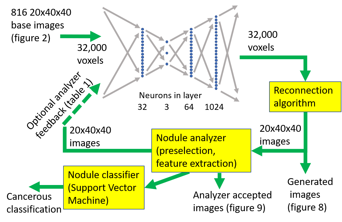
After a trained generator network produces images which are reconnected and validated by the nodule analyzer, a new training set may optionally be created for the next round of training iterations of the autoencoder. Figure 4 diagrams the data loop between the autoencoder and the nodule analyzer. We explored various approaches for augmenting the training set, but ultimately found that our best results came from proper autoencoder sizing and training with only the 816 base images created by adding guided training examples to the original 51 seed images. Although the image feedback into the training set did not improve the LuNG system, we include the description and results to illustrate the drawbacks of the approach.

We were motivated to explore augmentation approaches because we wanted to learn if adding accepted nodules to the training set could improve network $Score$ results by improving $FtDist$. One of the approaches used images from one trained network to augment a second trained network, similar to the multi-adversarial networks discussed in [17]. The intent of this approach is to improve the breadth of the feature space used to represent all legal nodules by importing images that were not generated by the network being trained.

We analyze the feedback approach we considered the best in detail in section IV. In this approach, we train the network for 50,000 iterations then generate 400 output images (less than half the size of the base set). We pass those images through the analyzer to insure they are considered legal and chose a single random reflection of each image to add to the training set. Because we are feeding in the image reflection, we did not find added value in having 2 networks trade generated images - the network itself was generating images whose reflections were novel to both its own feature network as input and its generator network as output. This training feedback is only done for 2 rounds of 25,000 training iterations and then a final 50,000 training iterations train only on the 816 base images.

The augmentation experiments explored whether having some training image variation helps fill the latent feature space with more variation on legal images. The intent of testing multiple approaches was to learn if an analyzer feedback behavior can be found that improves the criteria LuNG is trying to achieve: novel images accepted by the analyzer.

IV Experimental Results

Using the $Score$ metric and its components introduced in section  III-D, we evaluated various network sizes, the analyzer feedback approaches discussed in section III-E, and the reconnection algorithm discussed in section III-C. Our naming for networks is given with underscores separating neuron counts between the fully connected layers, so 32_3_64_1024 is a network with 4 hidden layers that have 32, 3, 64, and 1024 neurons respectively. As seen by referencing tables I and II, depending on the metric which is rated as most important, different architectures would be recommended.

IV-A Results for reconnection, feedback options, and depth

Table I shows training results for some of the feedback options discussed in section III-E. The networks in this table did not use the reconnection algorithm discussed in section III-C, so ’illegal’ inputs to the analyzer could occur, reducing the acceptance rate. The MSE column shows 1000 times the mean squared error per voxel for the autoencoder when given the 51 original seed nodules as inputs and targets. The ”AC%” column shows what percentage of 400 images randomly generated by the generator network were accepted by the analyzer. The ”FtDist” column shows the average minimum distance in analyzer feature space from any image to a seed image. The ”FtMMSE” column shows the average mean squared error of all 12 analyzer features between the images and the 51 seed images. ”No reflections” is one of our feedback options referring to using the accepted images from the analyzer directly in the training set. ”multiple” feedback refers to using 2 autoencoders and having each autoencoder use the accepted images that were output by the other. Using this table and other early results, we observed that the network with no analyzer feedback had overall good metrics, although the FtDist column indicating the novelty of images generated was lower than we would prefer, so we weighed ${FtDist}$ heavier in our final scoring of networks as we explored network sizing.

TABLE I: Key metrics for networks without reconnection

Network parameter testing (2 run average after 6 rounds)
Parameters	AC%	MSE	FtDist	FtMMSE
16_4_64_256_1024	54	0.03	1.75	0.07
No Feedback
16_4_64_256_1024	44	0.03	2.23	0.21
FB: no reflections
16_4_64_256_1024	36	0.05	2.43	0.26
FB: no reflections, multiple
16_4_64_256_1024	29	0.04	2.68	0.45
FB: 4 reflections, multiple

Table II shows experiments in which the reconnection algorithm was used. When using the reconnection algorithm, the analyzer always has a full set of 400 images to consider for acceptance, leading to higher acceptance rates. This table includes data on the number of raw generator output images which were clean when generated (one fully connected component) and the number that were inverted (white background with black nodule shape). The fact that deeper generation networks sometimes resulted in inverted output images is an indication that they have too many degrees of freedom and contributed to the decision to limit the depth of our autoencoder. The ”1 reflection” feedback label refers to having a single reflected copy of each accepted image used to train the autoencoder for 2 of the 6 rounds. This ”1 reflection” feedback was our most promising approach as described in section III-E.

TABLE II: Key metrics for networks using reconnection algorithm

Network parameter testing (2 run average after 6 rounds)
Parameters	AC%	MSE	FtDist	Clean	Invert
64_4_64_1024, No Feedback	85	0.08	1.78	109	0
64_4_64_1024, 1 reflection	64	0.06	3.13	63	0
64_4_64_256_1024, No Feedback	80	0.02	1.96	117	2
64_4_64_256_1024, 1 reflection	61	0.03	4.11	77	6.5

From the results in these 2 tables and other similar experiments, we concluded that the approach in section III-E, which used analyzer feedback for 2 of the 6 training rounds, had the best general results of the 4 feedback approaches considered. Also, the approach in section III-C, which will reconnect and repair generator network outputs, yielded 3D images preferable to the legal subset left when the algorithm was not applied. The results of these explorations informed the final constants that we used to create the $Score$ metric for rating networks as described in section III-D.

IV-B Results for tuning network sizes

We analyzed neuron counts as well as total number of network layers using $Score$. We tested multiple values for the neuron counts in each layer and figure 5 shows the results for testing the dimensions in the latent feature space. As can be seen, from the networks tested, the network which yielded the highest score of 176 was 32_3_64_1024, which is the network used to generate the nodule images shown in section IV-D.

Our final network can train on our data in an acceptable amount of time. Even though our experiments gathered significant intermediate data to allow for image feedback during training, the final 32_3_64_1024 network can be trained in approximately 2 hours. Our system for training has 6 Intel Xeon E5-1650 CPUs at 3.6GHz and an Nvidia GeForce GTX 1060 6GB GPU. Those 2 hours break down as: 10 minutes for creation of 816 base images from 51 seed images, 80 minutes to train for 150,000 epochs on the images, 20 minutes to generate and connect 400 nodules, and 10 minutes to run the analyzer on the nodules. Code tuning would be able to improve the image processing parts of that time, but the training was done using PyTorch [18] on the GPU and is already highly optimized. When generating images for practical use, we would recommend training multiple networks and using the results from the network that achieved the highest score.

Figure 5: $Score$ comparisons between networks that use 816 base images with no analyzer feedback for 150,000 training iterations versus networks that trained for 25,000 iterations on the base images, then added 302 generated nodules to train for 25,000 iterations, then added a different 199 generated nodules to train for 25,000 iterations, and then finished with 75,000 training iterations with no feedback.

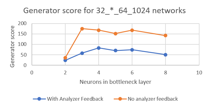
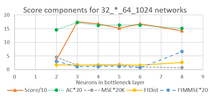
Figure 6 shows the components of $Score$ for the final parameter analysis we did on the network. Note that the MSE metric (mean squared error of the network on training set) continues to decrease with larger networks, but $Score$ is optimal with 3 bottleneck latent feature neurons. Our intuition is that limiting our network to 3 bottleneck neurons results in most of the available degrees of freedom being required for proper image encoding. As such, using a $-1$ to $1$ uniform random distribution as the prior distribution for our generative network creates a variety of acceptable images. The $Score$ metric helps us to tune the system such that we do not require VAE techniques to constrain our random image generation process, although such techniques may be a valuable path for future research.

Figure 6: There are 4 components used to compute the network score. The component values are scaled as shown so that they can all be plotted on the same scale.

IV-C Latent feature results

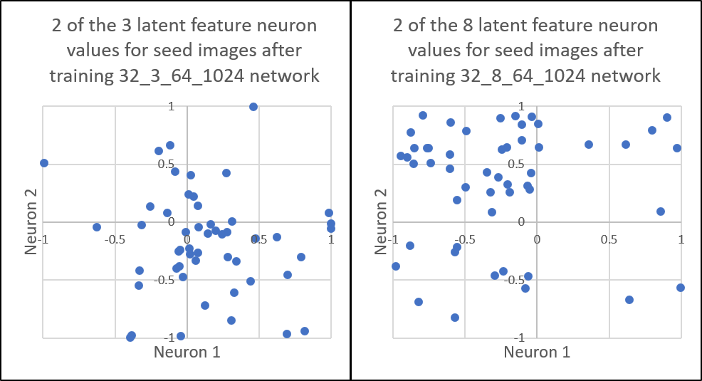
To visualize the weaknesses of too many bottleneck neurons in our autoencoder network, we plot the 51 seed nodule positions in the latent feature space in figure 7. To save space, we only present 2 of the 3 neurons for the final trained network, and we compare their positions to 2 of the 8 neurons from a trained network with 8 bottleneck neurons.

For the network with 3 bottleneck neurons, the plot shows that the 51 seed nodules are relatively well distributed in the 4 quadrants of the plot and the full range of both neurons is used to represent all the input images. For the network with 8 bottleneck neurons, most of the seed nodules map to the upper left quadrant in the plot and the full range of the 2 neurons is not used. This is a symptom of having a network with more degrees of freedom than needed to represent the nodule training space. Our intuition is that this contributes to the high ${FtM\!M\!S\!E}$ measurements shown in figure 6 for a network with 8 bottleneck neurons. The figures also show how a random -1 to 1 uniform range for our generator will likely result in a higher acceptance rate for images generated with 3 bottleneck neurons versus 8 bottleneck neurons.

Figure 7: Distribution of images in feature space after training with no feedback

IV-D Image results

The images shown in this section are from a network with 4 hidden layers with 32, 3, 64, and 1024 neurons. The network was trained without analyzer feedback and the output is processed to guarantee fully connected nodules.

Figure 8 shows the quality of 3D nodules our network can produce with 6 steps through the 3D bottleneck neuron latent feature space starting at the 2nd nodule from figure 2 and ending at the 4th nodule. First, note that the learned images for the start and end nodules are very similar to the 2nd and 4th input images, validating the MSE data that the network is correctly learning the seed nodules. The 4 internal step images have some relation to the start and end images but depending on the distance between the 2 nodules in latent feature space a variety of shapes may be involved in the steps.

Figure 8: 6 steps through 3D latent feature space between original nodules 2 and 4 from figure 2

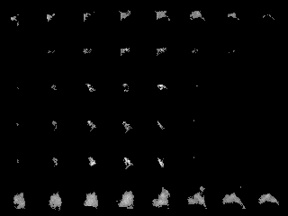
Figure 9 shows 6 images generated by randomly selecting 3 values between -1 and 1 for the latent feature inputs to the generator network and then being processed by the analyzer to determine acceptance. When using the network to randomly generate nodules (for classification by a trained specialist or training automated classifiers), this is an example of quality final results.

Figure 9: 6 images generated using uniform distribution from 3D feature space after passing nodule analyzer

IV-E Image quality for training

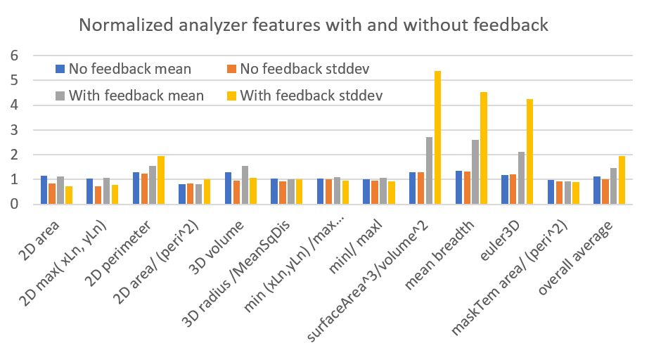
Figure 10 shows the 12 features that are used by the nodule analyzer and demonstrates another key success of our full approach. Characteristics like volume, surface area, and other values are used. We normalized the mean and standard deviation of each feature to 1.0 and the figure shows that the mean and standard deviation of the generated nodules for all 12 features stays relatively close to 1 for our proposed network with no analyzer image feedback. However, when feedback is used, one can see that the nodule features which have some deviation from the mean get amplified even though the analyzer tries to accept nodules in a way that maintains the same mean. For example, ”surface area³/volume²” is a measure of the compactness of a shape; the generated images from the network with no feedback tended to have higher surface area to volume than the seed images, and when these images were used for further training the generated images had a mean that was about 2.6 times higher than the seed images and a much higher standard deviation.

Figure 10: Computed 3D features from nodule analyzer. Our proposed method avoids the deviations shown by the grey and yellow bars.

Figure 11: Classifier distances to positive and negative centroids of SVM for 1000 analyzer accepted network generated samples. Nodules closer to positive than negative centroid after support vectors are applied are more likely cancerous.

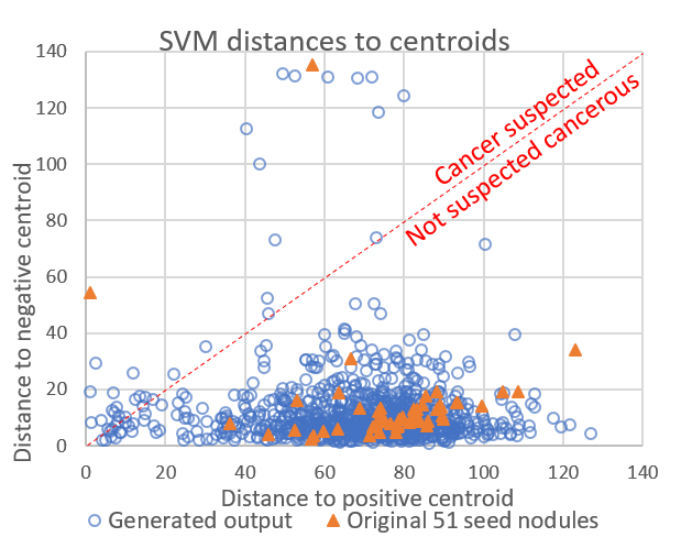
The ALNSB classifier we interact with uses a support vector machine to map images onto a 2D space representing distances to positive (suspicious) or negative (non-cancerous) centroids. Figure 11 shows the positive and negative centroid distances for the seed data and 1000 samples of analyzer accepted generated data. Nodules that have a smaller distance to the positive centroid than to the negative centroid are classified as likely cancerous. The general distribution of generated images fits the shape of the seed images rather well, and there is a collection of nodules being generated near the decision line between cancerous and non-cancerous, allowing for improved training based on operator classification of the nodules. Even though the original seed dataset only included 2 nodules eventually classified as potentially cancerous, our approach can use shape data from all 51 nodules to create novel images that can be useful for improving an automated screening system. Note that these centroid distances themselves are not part of the 12 features that are used to filter the nodules, so this figure validates our approach to create images usable for further automated classification work.

V Related Work

Improving automated CT lung nodule classification techniques and 3D image generation are areas that are receiving significant research attention.

Recently, Valente et al. provided a good overview of the requirements for Computer Aided Detection systems in medical radiology and they survey the status of recent approaches [2]. Our aim is to provide a tool which can be used to improve the results of such systems by both decreasing the false positive rate and increasing the true positive rate of classifiers through the use of an increase in nodules for training and analysis. Their survey paper discusses in detail preprocessing, segmentation, and nodule detection steps similar to those used in the ALNSB nodule analyzer/classifier which we used in LuNG.

Li et. al provide a thorough overview of recent approaches to 3D shape generation in their paper ”GRASS: Generative Recursive Autoencoders for Shape Structures” [10]. While we do not explore the design of an autoencoder with convolutional and deconvolutional layers, the same image generation quality metrics that we teach could be used to evaluate such designs. Tradeoffs between low reproduction error rates and overfitting would have to be considered when setting the network depth and feature map counts in the convolutional layers.

Durugkar et al. describe the challenges of training GANs well and discuss the advantages of multiple generative networks trained with multiple adversaries to improve the quality of images generated [17]. LuNG explored using multiple networks during image feedback experiments. Larsen et al. [19] teach a system which combines a GAN with an autoencoder which could be a basis for future work introducing GAN methodologies into the LuNG system by preserving our goal of generating shapes similar to existing seed shapes.

VI Conclusion

To produce quality image classifiers, machine learning requires a large set of training images. This poses a challenge for application areas where large training sets are rare, such as for new medical techniques using computer-aided diagnosis of cancerous lung nodules.

In this work we developed LuNG, a lung nodule image generator, allowing us to augment the training dataset of image classifiers with meaningful (yet computer-generated) lung nodule images. Specifically, we have developed an autoencoder-based system that learns to produce 3D images with features that resemble the original training set. LuNG was developed using PyTorch and is fully implemented and automated. We have shown that the 3D nodules generated by this process visually and numerically align well with the general image space presented by the limited set of seed images.

Acknowledgment

This work was supported in part by the U.S. National Science Foundation award CCF-1750399.

References

- [1] R. L. Siegel, K. D. Miller, and A. Jemal, “Cancer statistics, 2017,” CA: A Cancer Journal for Clinicians, vol. 67, no. 1, pp. 7–30, 2017. [Online]. Available: http://dx.doi.org/10.3322/caac.21387
- [2] I. R. S. Valente, P. C. Cortez, E. C. Neto, J. M. Soares, V. H. C. de Albuquerque, and J. a. M. R. Tavares, “Automatic 3D pulmonary nodule detection in CT images,” Comput. Methods Prog. Biomed., vol. 124, no. C, pp. 91–107, Feb. 2016. [Online]. Available: http://dx.doi.org/10.1016/j.cmpb.2015.10.006
- [3] S. Kommrusch and L.-N. Pouchet, “Synthetic lung nodule 3D image generation using autoencoders,” in Deep learning through sparse and low-rank modeling, Z. Wang, T. S. Huang, and Y. Raymond, Eds. Academic Press, 2019.
- [4] Q. Li, F. Li, and K. Doi, “Computerized detection of lung nodules in thin-section CT images by use of selective enhancement filters and an automated rule-based classifier,” Acad Radiol, vol. 15, no. 2, pp. 165–175, Feb 2008.
- [5] M. J. M. Chuquicusma, S. Hussein, J. Burt, and U. Bagci, “How to fool radiologists with generative adversarial networks? a visual turing test for lung cancer diagnosis,” ArXiv, Oct. 2017.
- [6] CDSC, “NSF Center for Domain-Specific Computing,” 2018, https://cdsc.ucla.edu.
- [7] J. Rong, P. Gao, W. Liu, Y. Zhang, T. Liu, and H. Lu, “Computer simulation of low-dose CT with clinical lung image database: a preliminary study,” in Society of Photo-Optical Instrumentation Engineers (SPIE) Conference Series, ser. Society of Photo-Optical Instrumentation Engineers (SPIE) Conference Series, vol. 10132, Mar. 2017, p. 101322U.
- [8] S. Shen, P. Rawat, L.-N. Pouchet, and W. Hsu, “Lung nodule detection C benchmark,” https://github.com/cdsc-github/Lung-Nodule-Detection-C-Benchmark, 2015.
- [9] C. Cummins, P. Petoumenos, Z. Wang, and H. Leather, “Synthesizing benchmarks for predictive modeling,” in Proc. of the 2017 International Symposium on Code Generation and Optimization, ser. CGO ’17. IEEE Press, 2017, pp. 86–99.
- [10] J. Li, K. Xu, S. Chaudhuri, E. Yumer, H. Zhang, and L. Guibas, “GRASS: Generative recursive autoencoders for shape structures,” ACM Transactions on Graphics (Proc. of SIGGRAPH 2017), vol. 36, no. 4, p. to appear, 2017.
- [11] C. Doersch, “Tutorial on variational autoencoders,” ArXiv, Jun. 2016.
- [12] Skymind, “GAN: A beginner’s guide to generative adversarial networks,” https://deeplearning4j.org/generative-adversarial-network, 2017.
- [13] D. P. Kingma and J. Ba, “Adam: A method for stochastic optimization,” ArXiv, Dec. 2014.
- [14] G. E. Hinton and R. R. Salakhutdinov, “Reducing the dimensionality of data with neural networks,” Science, vol. 313, no. 5786, pp. 504–507, 2006.
- [15] S. S. Haykin, Neural networks and learning machines, 3rd ed. Pearson Education, 2009.
- [16] P. C. Mahalanobis, “On the generalized distance in statistics,” in Proceedings of the National Institute of Sciences of India, ser. Proceedings of the National Institute of Sciences of India, vol. 2, 1936, pp. 49–55.
- [17] I. Durugkar, I. Gemp, and S. Mahadevan, “Generative multi-adversarial networks,” ArXiv, Nov. 2016.
- [18] A. Paszke, S. Gross, S. Chintala, and G. Chanan, “PyTorch,” https://github.com/pytorch/pytorch, 2017.
- [19] A. Boesen Lindbo Larsen, S. Kaae Sønderby, H. Larochelle, and O. Winther, “Autoencoding beyond pixels using a learned similarity metric,” ArXiv, Dec. 2015.