ShapeSearch: A Flexible and Efficient System for Shape-based Exploration of Trendlines

Abstract.

Identifying trendline visualizations with desired patterns is a common task during data exploration. Existing visual analytics tools offer limited flexibility, expressiveness, and scalability for such tasks, especially when the pattern of interest is under-specified and approximate. We propose ShapeSearch, an efficient and flexible pattern-searching tool, that enables the search for desired patterns via multiple mechanisms: sketch, natural-language, and visual regular expressions. We develop a novel shape querying algebra, with a minimal set of primitives and operators that can express a wide variety of ShapeSearch queries, and design a natural-language and regex-based parser to translate user queries to the algebraic representation. To execute these queries within interactive response times, ShapeSearch uses a fast shape algebra execution engine with query-aware optimizations, and perceptually-aware scoring methodologies. We present a thorough evaluation of the system, including a user study, a case study involving genomics data analysis, as well as performance experiments, comparing against state-of-the-art trendline shape matching approaches—that together demonstrate the usability and scalability of ShapeSearch.

1. Introduction

Identifying patterns in trendlines or line charts is an integral part of data exploration—routinely performed by domain experts to make sense of their datasets, gain new insights, and validate their hypotheses. For example, clinical data analysts examine trends of health indicators such as temperature and heart-rate for diagnosis of medical conditions (gotz2014methodology, ); astronomers study the variation in properties of galaxies over time to understand the history and makeup of the Universe (morganson2018dark, ); biologists analyze gene expression patterns over time to study biological processes (wagner2005genome, ; lee2019you, ); and financial analysts study trends in stock prices to predict future behavior (ge1998pattern, ). Due to the lack of extensive programming experience, these domain experts typically perform manual exploration, tediously examining trendlines one at a time until they find ones that match their desired shape or pattern, e.g., gene expressions that rise and then become stable.

Recent work has proposed tools that let users interactively search for desired patterns (zenvisagevldb, ; qetchchi, ; timesearcher, ; googlecorrelate, ). However, as we will discuss below, these tools expect users to search in highly constrained ways, and, in addition, are overly rigid in how they assess a match. Most tools expect users to specify a complete and exact trendline as input usually by sketching it on a canvas, followed by computing distances between this exact trendline and several candidate trendlines to identify matches. As a result, these tools are unable to support search when the desired shape is under-specified or approximate, e.g., finding stocks whose prices are decreasing for some time, followed by a sharp rise, with the position and intensity of movements being left unspecified, or when the desired shape is complex, e.g., finding gene expression profiles where there is an unspecified number of peaks and valleys followed by a flattening out. Some data mining tools provide the ability to search for patterns in time series, e.g., (psaila1995querying, ; garofalakis1999spirit, ), but require heavy precomputation, limiting ad-hoc exploration, in addition to suffering from the same limitations in flexibility as the visualization tools. Yet another alternative for domain experts with programming expertise is to write code to perform this flexible match, but writing code for each new use-case, followed by manual optimization is often as tedious as manual searching of visualizations to find patterns.

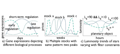
Figure 1. Shapes characterizing real world phenomena

We present ShapeSearch, a visual data exploration system that supports multiple novel mechanisms to express and effortlessly search for desired patterns in trendlines. Before describing ShapeSearch, we first characterize typical trendline pattern-based queries.

1.1. Characterizing Shape Queries

The design of ShapeSearch has been motivated by case studies and use-cases from domains such as genomics, astronomy, battery science, and finance, using a process similar to our earlier work (lee2019you, ). We also collected a corpus of about $250$ natural language queries via Mechanical Turk (mturk), where we asked crowd workers to describe patterns in trendline visualizations collected from real world datasets. We highlight the key characteristics of pattern matching tasks, based on our discussions with domain experts and analysis of mturk queries below.

Fuzzy Matching. Domain experts typically search for patterns (i) that are approximate, and are often not interested in the specific details or local fluctuations as much as the overall shape, and (ii) they often do not specify or even know the exact location of the occurrence of patterns. For example, biologists routinely look for structural changes in gene expression, e.g., rising and falling at different times (Figure 1a). Structural changes characterize internal biological processes such as the cell cycle or circadian rhythms, or external perturbation, such as the influence of a drug or presence of a disease. Similarly, many crowd workers tend to describe trendlines using high level patterns such as increasing and then decreasing, without being precise about locations and/or features of the changes.

Combination of Multiple Simple Patterns. We notice that both domain experts as well as crowd workers often describe complex patterns using a combination of multiple simple ones. Each individual pattern is typically described using words such as ”increasing”, ”stable”, or ”falling”, which are easy to state in natural language but hard to specify using existing query languages. Moreover, pattern matching tasks in many domains often go beyond finding a sequence of patterns, requiring arbitrary combinations, e.g., disjunction, conjunction, or quantification, with varying location or width constraints. Examples include finding stocks with at least $2$ peaks within a span of $6$ months, e.g., the so-called ”double/triple top” patterns that indicate future downtrends (investopedia, ), or finding cities where the temperature rises from November to January and falls during May to July, such as Sydney.

Ad hoc and Interactive. Pattern-based queries are often defined on-the-fly during analysis, based on other patterns observed. For instance, biologists often search for a pattern in a group of genes similar to a pattern recently discovered in another group (lee2019you, ). Similarly, astronomers monitor the shape of the luminosity trends of stars over time to search for and characterize new planetary objects (Figure 1c). For example, a dip in brightness often indicates a planetary object passing between the star and the telescope. In order to limit comparison of patterns over similar duration (i.e., the X axis) or over value ranges (i.e, the Y axis), it is common to apply constraints while pattern matching. Examples include searching for changes in buying and selling patterns of stock or house prices in a specific range or duration. As such, some tools, e.g., TimeSearcher (timesearcher, ), allow interactive specification of constraints, however the pattern matching is still precise or value-based.

1.2. Our Approach

To satisfy the aforementioned characteristics, ShapeSearch makes three contributions.

(a) ShapeSearch incorporates an expressive shape query algebra that abstracts key shape-based primitives and operators for expressing a variety of desired trendline patterns. The most powerful feature of this algebra is its capability for “fuzzy” matching, allowing approximate and inexact pattern specification, without compromising on the needs of occasional precise queries. We developed this algebra after discussions with domain experts, as well as studying mturk pattern queries, as mentioned earlier.

(b) Unfortunately, naïvely executing these fuzzy queries is extremely slow, requiring an expensive evaluation of all possible ways of matching each candidate trendline to the query to select the best one. We propose a dynamic programming-based optimal algorithm that reuses computation to provide substantial speed-ups, and show that even this algorithm can be prohibitively slow for interactive ad-hoc exploration. We then develop a novel perceptually-aware bottom-up algorithm that incrementally prunes the search space based on patterns specified in the query, providing a $\textbf{40}\times$ speedup with over 85% accuracy, compared to the optimal approach.

Table 1. Comparison between specification mechanisms

Mechanism	Intuitiveness	Control	Expressiveness
Natural language	high	low	high
Sketch	high	high	low
Regex	low	high	high

(c) Finally, to accommodate a range of needs without sacrificing the expressiveness of the algebra, ShapeSearch supports three query specification mechanisms (Table 1): sketching on a canvas, natural language, and regular expressions (regex for short). All specification mechanisms are translated to the same shape query algebra representation, and can be used interchangeably, as user needs evolve.

Next, we explain how a user interacts with ShapeSearch.

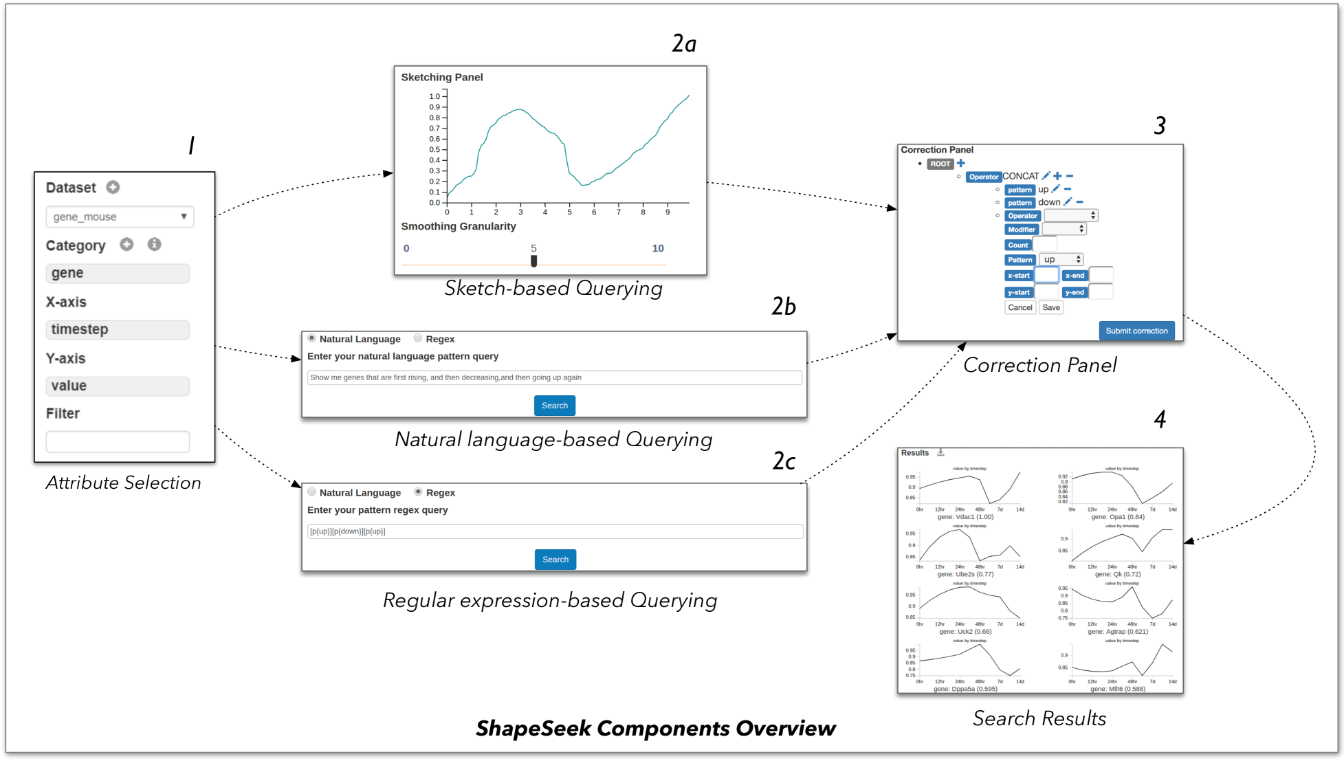
(a) ShapeSearch Interface

Symbol	Name	Type
x.s	START X VALUE	Location Sub-Primitive
y.s	START Y VALUE	Location Sub-Primitive
x.e	END X VALUE	Location Sub-Primitive
y.e	END Y VALUE	Location Sub-Primitive
v	SKETCH	Location Sub-Primitive
p	PATTERN	Primitive
$\color[rgb]{0,.5,.5}\otimes$	CONCAT	Operator
$\color[rgb]{.75,.5,.25}\odot$	AND	Operator
$\color[rgb]{1,.5,0}\oplus$	OR	Operator

(b) Algebra Primitives and Operations

(c) ShapeQuery AST

Figure 2. a) ShapeSearch Interface, consisting of six components. Box 1: Data upload, attributes selection, and applying filter constraints; Box 2: Query specification—Box 2a: Sketching canvas, Box 2b: Natural language query interface, and Box 2c: Regular expression interface; Box 3: Correction panel; and Box 4) Results panel. b) Primitives and Operators in ShapeQuery. c) Abstract tree representation of ShapeQuery [ p=up]$\color[rgb]{0,.5,.5}\otimes$[p=down]$\color[rgb]{0,.5,.5}\otimes$(([ p=up]$\color[rgb]{0,.5,.5}\otimes$[ p=down])$\color[rgb]{1,.5,0}\oplus$[ p=flat])

1.3. ShapeSearch System Overview

Figure 2(a) depicts the ShapeSearch interface, with an example query on genomics data. Here, a user wants to search for genes that get suppressed due to the influence of a drug, with a specific shape in their gene expression—first rising, then going down, and finally rising again—with three patterns: up, down, and up, in a sequence. To search for this shape, the user first loads the dataset (bult2008mouse, ), via a form (Figure 2(a) box 1), and then selects the space of trendline visualizations to explore by setting parameters: $x$ axis as time, $y$ axis as expression values, and category/$z$ axis as gene. ShapeSearch generates a trendline visualization for each unique value of the $z$ axis. Thus, the $z$ axis defines the space of visualizations over which we match the shape. Once the data is loaded, the user can leverage three mechanisms for shape query specification:

Sketching on Canvas. By drawing the desired shape as a sketch on the canvas (Figure 2(a) box 2a), the user can search for trendlines that precisely match this sketch, using a distance measure such as Euclidean distance or Dynamic Time Warping (dtw, ). ShapeSearch outputs visualizations similar to the drawn sketch in the results panel (Figure 2(a) box 4).

Natural Language (NL). For searching for approximate pattern matches, users can use natural language. For instance, in Figure 2(a) box 2b, the desired genomics shape can be expressed as “show me genes that are rising, then going down, and then increasing”. Similarly, scientists analyzing cosmological data can search for supernovae (bright stellar explosions) using “find me objects with a sharp peak in luminosity”.

Regular Expression (regex). For queries that involve complex combinations of patterns that are difficult to express using natural language or sketch, the user can issue a regular expression-like query that directly maps to the internal ShapeQuery algebraic representation, consisting of ShapeSearch primitives and operations. While sketch is typically used for precise matching, ShapeSearch also allows approximate matching via sketch by constructing a regex from a sketch (see Appendix A.2).

The ShapeSearch back-end parses and translates all queries into the ShapeQuery algebra before execution. For translating natural language queries, ShapeSearch supports a sophisticated parser that uses a mix of learning and rules for resolving syntactic and semantic ambiguities. After translation, the backend forwards the regex representation of the query to the user for validation or correction (Figure 2(a) Box 3). The validated query is finally optimized and executed, and the top visualizations that best match the ShapeQuery are presented in the results panel (Figure 2(a) Box 4).

Paper Outline. We explain the three key components of ShapeSearch in the following sections. In Section 2, we give an overview of the ShapeQuery algebra, along with its primitives and operators. In Section 3, we discuss the challenges in executing fuzzy shape queries and how we make ShapeSearch scale to large collections of trendlines. We briefly explain the natural language translation in Section 4. We describe our performance experiments evaluating the efficiency and accuracy of the ShapeSearch pattern execution engine in Section 5. We present a user study in Section 6 and a genomics case study in Section 7, evaluating the expressiveness, effectiveness, and usability of ShapeSearch. We presented an early version of ShapeSearch in a demo paper (shapesearchdemo, ).

2. ShapeQuery Algebra

We give an overview of ShapeQuery, a structured query algebra, motivated from use-cases in real domains as well as our analysis of the crowdsourced pattern queries.

Overview. The ShapeQuery algebra consists of a minimal set of primitives and operators for declaratively expressing a rich variety of patterns, while supporting the three characteristics of pattern-matching tasks described in the introduction. At a high level, a ShapeQuery represents a shape as a combination of multiple simple patterns. A simple pattern can either be precise with specific location constraints, e.g., matching $y=x$ between $x=2$ to $x=6$, or fuzzy, e.g., roughly increasing, where the notion of the pattern is approximate and its location unspecified. Each simple pattern along with its precise or imprecise constraints is called a ShapeSegment. Complex shapes, e.g., rising and then falling, are formed by combining multiple ShapeSegments using one or more operators. One can search for multiple patterns in a sequence (concat, $\color[rgb]{0,.5,.5}\otimes$) or matching the same sub-region of the trendline (and, $\color[rgb]{.75,.5,.25}\odot$), or one of many patterns matching a sub-region (or, $\color[rgb]{1,.5,0}\oplus$), described later.

As an example,“rising from $x$=$2$ to $x$=$5$ and then falling” can be translated into a ShapeQuery [x.s=2,x.e=5, p=up] $\color[rgb]{0,.5,.5}\otimes$[p=down] consisting of two ShapeSegments separated by a $\color[rgb]{0,.5,.5}\otimes$ operator. The first ShapeSegment captures “rising from $x=2$ to $x=5$”; the second expresses a “falling” pattern. Since the second must “follow” the first, the two ShapeSegments are combined using the CONCAT operator, denoted by $\color[rgb]{0,.5,.5}\otimes$. We now describe the shape primitives and operators that constitute ShapeQuery algebra. Table 2(b) lists these primitives and operators.

2.1. Shape Primitives and Operators

A ShapeSegment is described using two high level primitives: LOCATION and PATTERN. ShapeSearch allows users to skip one or more of these primitives in their query. The LOCATION values can be skipped in order to match the PATTERN anywhere in the trendline. Similarly, users can input the exact trendline to match, or the endpoints of the ShapeSegments to match without specifying the PATTERN. We describe each of these supported primitives.

Specifying LOCATION. LOCATION defines the endpoints of the sub-region of the trendline between which a pattern is matched: starting X/Y coordinate (x.s/y.s), ending X/Y coordinate (x.e/y.e). For example, [x.s=2,x.e=10, y.s=10,y.e=100] is a simple ShapeQuery to find trendlines whose trend between $x$=$2$ to $x$=$10$ is similar to the line segment from ($2,10$) to ($10,100$). Users can also draw a sketch to find trendlines similar to the sketch, a functionality supported in other tools alluded to in the introduction (zenvisagevldb, ; timesearcher, ; googlecorrelate, ). ShapeSearch translates the pixel values of the user-drawn sketch to the domain values of the X and Y attributes, and adds the transformed vector of $(x,y)$ values as a vector $v$ in the ShapeQuery. As an example, the ShapeQuery [v=(2:10,3:14,...,10:100)] finds trendlines that have precisely similar values to $v$ using a distance measure, e.g., Euclidean distance, or dynamic time warping (dtw, ).

Specifying PATTERN. PATTERN defines a trend or a semantic feature in a sub-region of the trendline. A number of basic semantic patterns, commonly used for characterizing trendlines, are supported, such as up, down, flat, or the slope ($\theta$) in degrees. For example [p=up] finds trendlines that are increasing, [p=45] finds trendlines that are increasing with a slope of about $45^{\circ}$, and [x.s=2,x.e=10, p=up] finds trendlines that are increasing from $x=2$ to $10$. Finally, one can use p=* to match any pattern and p=empty to ensure that there are no points over the sub-region.

Table 2. Examples of ShapeQueries

Pattern	ShapeQuery
Increasing from 2 to 5 and then decreasing	[ p=up, x.s=2, x.e=10]$\color[rgb]{0,.5,.5}\otimes$[ p=down]
Decreasing or increasing anywhere	[ p = *]$\color[rgb]{0,.5,.5}\otimes$( p=up$\color[rgb]{1,.5,0}\oplus$ p=down) $\color[rgb]{0,.5,.5}\otimes$[ p = *]
Increasing at 45, decreasing at 60 and then becomes flat	[ p = 45]$\color[rgb]{0,.5,.5}\otimes$[ p = -60]$\color[rgb]{0,.5,.5}\otimes$[ p = flat]
Decreasing over a width of 3 points:	[ x.s=., x.e=.+3, p=down]
Increasing at least once and at most 5	[ p=up, q=1,5]
W shaped pattern	[ p=-45]$\color[rgb]{0,.5,.5}\otimes$[ p = 60]$\color[rgb]{0,.5,.5}\otimes$[ p=-45]$\color[rgb]{0,.5,.5}\otimes$[ p = 60]
Specific sketch	[ v = (2:10,3:14,…,10:100)]
Shape whose trend is increasing relatives its own trend before some point in the past (e.g, inverted bell shaped)	[ p=down]$\color[rgb]{0,.5,.5}\otimes$[ p ¿ $$-$.p]

Table 3. Pattern Scores

P	Score
up	$\frac{2\cdot tan^{-1}(slope)}{\pi}$
down	$-\frac{2\cdot tan^{-1}(slope)}{\pi}$
flat	$(1.0-\lVert\tfrac{4\cdot tan^{-1}(slope)}{\pi}\rVert)$
$\theta=x$	$(1.0-\lVert\tfrac{2\cdot tan^{-1}(slope-x))}{(\pi-\rVert tan^{-1}(x\rVert)}\rVert)$
$*$	1
empty	-1
$v$	$L_{2}$ norm (configurable)

Table 4. Operator Scores

O	Score
$\color[rgb]{0,.5,.5}\otimes$	$\sum_{i=1}^{k}score_{i}/k$
$\color[rgb]{.75,.5,.25}\odot$	$min(score_{1},...,score_{k})$
$\color[rgb]{1,.5,0}\oplus$	$max(score_{1},...,score_{k})$

Combining PATTERNs. ShapeQuery supports three operators to combine ShapeSegments:

• CONCAT ($\color[rgb]{0,.5,.5}\otimes$) specifies a sequence of two or more ShapeSegments. For example, using [p=up]$\color[rgb]{0,.5,.5}\otimes$[p=down] one can search for genes that are first rising, and then falling. Note that $\color[rgb]{0,.5,.5}\otimes$ is one of the most frequently used operations, and we sometimes omit $\color[rgb]{0,.5,.5}\otimes$ between ShapeSegments, e.g, [p=up][p=down], to make it succinct to describe.

• AND ($\color[rgb]{.75,.5,.25}\odot$) simultaneously matches multiple patterns in the same sub-region of the trendline. Unlike CONCAT, all of the patterns must be present in the same sub-region. For example, one can look for genes whose expression values rise twice but do not fall more than once within the same sub-region.

• OR ($\color[rgb]{1,.5,0}\oplus$) searches for one among many patterns in the same sub-region of the trendline, picking the one that matches the sub-region best. For example, one can search for genes whose expressions are either up- or down-regulated.

Note that when the same operator is specified consecutively, ShapeSearch fuses them into one, hence all operators can take two or more operands. For example, [p=up] $\color[rgb]{0,.5,.5}\otimes$[p=down] $\color[rgb]{0,.5,.5}\otimes$[p=down] is parsed as a single $\color[rgb]{0,.5,.5}\otimes$ operation with three operands [p=up], [p=down], and [p=down].

Multiple operations are often used in a given ShapeQuery. ShapeSearch follows left to right precedence order for execution of the operations. However, sub-expressions can be nested using parentheses $()$ to specify precedence as in mathematical expressions. In Figure 2(c), we depict how ShapeSearch parses a complex ShapeQuery [ p=up]$\color[rgb]{0,.5,.5}\otimes$[ p=down] $\color[rgb]{0,.5,.5}\otimes$(([ p=up]$\color[rgb]{0,.5,.5}\otimes$[ p=down])$\color[rgb]{1,.5,0}\oplus$[p=flat]) into an Abstract Syntax Tree (AST) representation.

Comparing Patterns. In some cases, one may want to compare the pattern in a ShapeSegment with the preceding or succeeding ShapeSegments. To support such use cases, ShapeSearch (i) allows a ShapeSegment to refer to the previous or the next ShapeSegment using $\$+$ or $\$-$ respectively, and (ii) compare patterns between the current and referred ShapeSegment using operations $>$, $<$, or $=$. For example, astronomers can issue a ShapeQuery [p=up]$\color[rgb]{0,.5,.5}\otimes$[ p ¡ $$-$.p] with $x$=time and $y$=luminosity (brightness) to search for celestial objects that were initially moving rapidly towards earth, but after some point either slowed down or started moving away. The second ShapeSegment [ p ¡ $$-$.p] ensures that the slope of brightness over time is less than that in the previous sub-region [p=up].

Similarly, one can set p ¡$\frac{1}{2}$$$-$.p to ensure the slope of second sub-region is $\leq\frac{1}{2}$ of the first. To avoid ambiguity in position reference and for efficient execution, ShapeSearch restricts $-based references to a simple CONCAT operation, i.e., across a sequence of patterns at the same level of nesting.

Expressing complex patterns. The aforementioned basic primitives and operators are powerful enough to express more complex ShapeSearch use-cases. We discuss three such complex patterns below, along with shortcuts for their easy specification.

1. Searching shapes of specific width. In some cases, users want to find specific shapes irrespective of their start location. For example, one may want to search for cities with maximum rise in temperature over a width of $3$ months. To express such queries, ShapeSearch supports the ITERATOR (.), e.g., [x.s=.,x.e=x.s+3,p=up] that iterates over all points in the trendline, setting each point as the start $x$ position, with the $x$ end position set to 3 units ahead. Internally, for a trendline of length $n$, this query can be rewritten as an OR operation over $(n-3+1)$ ShapeSegments, where, for the $i$th ShapeSegment, x.s=i and x.e=i+3.

2. Quantifiers. One can search for trendlines where a pattern occurs a specific number of times using quantifiers, denoted by q. For example, [p=up,q={1,2}] can be used to search for trendlines where there is an increasing pattern at least once and at most twice. Quantifiers can be internally rewritten using an OR of one or more CONCAT operations. For example, the above query is rewritten as ([p=*] $\color[rgb]{0,.5,.5}\otimes$[p=up]$\color[rgb]{0,.5,.5}\otimes$[p=*])$\color[rgb]{1,.5,0}\oplus$([p=*]$\color[rgb]{0,.5,.5}\otimes$[p=up]$\color[rgb]{0,.5,.5}\otimes$[p=*] $\color[rgb]{0,.5,.5}\otimes$[p=up]$\color[rgb]{0,.5,.5}\otimes$[p=*]).

3. Nesting A combination of patterns can be constrained to be within a specific sub-region by specifying them as a value of the PATTERN primitive. For example, to search for stocks that increased anytime between February to October, we can use nesting as follows: [x.s=2,x.e=10, p=([p=*][p=up][p=*])]. This can be rewritten using CONCAT operations as follows: [x.s=2,p=*]$\color[rgb]{0,.5,.5}\otimes$[p=up]$\color[rgb]{0,.5,.5}\otimes$[p=*]$\color[rgb]{0,.5,.5}\otimes$[x.s=10,p=*].

4. Scale invariant matching. One can automatically search for shapes at varying granularity of x-scales and degree of smoothing. For example, for [p=*]$\color[rgb]{0,.5,.5}\otimes$[p=up] $\color[rgb]{0,.5,.5}\otimes$[p=down]$\color[rgb]{0,.5,.5}\otimes$[p=*], ShapeSearch searches for [p=up] and then [p=down] at all possible scales and selects the one that leads to the best match. To do so, ShapeSearch uses efficient algorithms that we describe in the subsequent sections.

As ShapeSearch evolves, it may support additional shortcuts to simplify the writing of frequently used complex patterns.However, all of the complex patterns as well as the shortcuts can be expressed using basic primitives and operations for their execution. Thus, we omit further discussion of complex patterns and limit ourselves to the semantics and efficient scoring of basic primitives and operators.

2.2. Formal semantics of ShapeQuery

We now formally define the semantics of ShapeQuery.

Given three dataset attributes $x$, $y$, and $z$,  ShapeSearch first generates a collection of trendlines $V$, one for each unique value of the $z$ attribute. Each trendline is a sequence of ($x$, $y$) values ordered by $x$. A ShapeQuery $Q$ operates on one trendline, $V_{i}$, at a time, and returns a real number, called score, between $-1$ to $+1$, i.e., $Q:V_{i}\rightarrow score$; $score\in[-1,1]$. The value of $score$ describes how closely $V_{i}$ matches $Q$, with $+1$ the best possible match, and $-1$ the worst.

The ShapeQuery Q operates on $V_{i}$ with the help of ShapeSegments ($S_{1},S_{2},\ldots,S_{n}$) and operators ($O_{1},O_{2},\ldots,O_{m}$). Each ShapeSegment, $S_{i}$ operates on $V_{i}^{p,q}$, a sub-region of $V_{i}$ starting at $p=x.s$ and ending at $q=x.e$ and returns a $score_{i}\in[-1,1]$ using scoring functions we describe subsequently. A common subclass of ShapeQueries are fuzzy ShapeQueries. A fuzzy ShapeQuery is a sequence of ShapeSegments where there is at least one ShapeSegment with missing or multiple possible values for $x.s$ or $x.e$. Thus, for fuzzy ShapeQueries, we try all possible values of $p$ and $q$, selecting the sub-region that leads to the best score. One or more ShapeSegments are combined using operators such as $\color[rgb]{0,.5,.5}\otimes$, $\color[rgb]{.75,.5,.25}\odot$, $\color[rgb]{1,.5,0}\oplus$. Formally, an operator $O_{i}$ takes as input the scores $score_{1},score_{2},\ldots,score_{n}$ from its $n$ input ShapeSegments and outputs another $score_{i}$ using scoring functions that capture the behavior of the operators. When combined via AND or OR operators, ShapeSegments may operate on overlapping sub-regions $V_{i}^{p,q}$, however, for CONCAT, the sub-regions must not overlap since CONCAT specifies a sequence of patterns. Next, we describe our scoring methodology.

2.3. Scoring Methodology

For supporting interactive response times, ShapeSearch needs to efficiently and effectively compute the match between a ShapeQuery $Q$ and a trendline $V_{i}$.

To satisfy both efficiency and effectiveness, ShapeSearch approximates each sub-region with a line, using the slope to quantify how closely it captures any given ShapeSegment. The line-based quantification is robust to noise or minor fluctuations, as is often intended in ShapeQueries. At the same time, lines are extremely fast to compute, requiring only a single pass on the data. As we explain shortly, lines over larger sub-regions can be quickly inferred from lines over over smaller ones, without additional passes. As the complexity of a pattern increases, the number of lines required to approximate it also increases. However, even for complex shapes, a small number of line segments is sufficient. Our study of patterns (e.g., double-bottom, triple-top) in finance (ge1998pattern, ) as well as mturk queries reveal that the maximum number of lines is usually small (typically less than $6$).

As depicted in Table 4, ShapeSearch uses different scoring functions for each pattern primitive that transforms the slope to a value in $[-1,1]$ using a $tan^{-1}$ function. For example, for an up pattern, the function returns a score between $[0,1]$ for all trendlines with slope from $0^{\circ}$ to $90^{\circ}$, a score of $[-1,0]$ for slopes $<0^{\circ}$ (opposite of up). Moreover, a change in trend from $10^{\circ}$ to $30^{\circ}$ is visually more noticeable than from $60^{\circ}$ to $80^{\circ}$, thus we capture this behavior using $tan^{-1}$ where the rate of increase in output decreases as the value of slope increases. Finally, we apply normalization, such as multiplying by $2/\pi$, to re-scale the output of $tan^{-1}$ between $-1$ and $1$. Thus, depending on the specified pattern primitive, ShapeSearch uses the corresponding scoring function to compute the score for that ShapeSegment. For a given ShapeSegment, if the location constraints are not met, we assign a score of -1, and ignore the rest of the primitives.

We state the following observation regarding the scoring of a single ShapeSegment.

Observation 2.1. The scoring of a ShapeSegment, as part of a ShapeQuery $Q$ without comparisons, on a sub-region $L$ can be done using the slope of the corresponding single line segment and the $x.s$, $x.e$, $y.s$, and $y.e$ values of the sub-region, independent of other sub-regions.

For a shape input as a sketch, users sometimes intend to perform precise matching. For such ShapeSegments we compute the score using L2 norm (Euclidean distance) between the drawn sketch and the trendline without fitting a line segment. The L2 norm can vary from 0 to $\infty$; therefore, we normalize the distance within [1, -1] using using Max-Min normalization (minmax, ). In addition, ShapeSearch allows users to use sketch for fuzzy matching where ShapeSearch fits a minimum number of lines to the sketch given an error threshold (adjustable via a slider), and automatically constructs a CONCAT operation of ShapeSegments, with one ShapeSegment for each line with the pattern corresponding the slope of the line. We provide more details on fuzzy matching using sketch in Appendix A.2.

For two contiguous ShapeSegments compared using $-references, ShapeSearch returns a single score as if they were one single ShapeSegment evaluated over their combined sub-region. Internally, ShapeSearch evaluates each of ShapeSegments over their corresponding sub-region independently and combines scores across the CONCAT appropriately. The score of the ShapeSegment that uses that $ reference is set to $+1$ if the constraint is satisfied, otherwise it is set to $-1$. For ease of explanation, we refer them as a single ShapeSegment for the rest of the paper.

The scores across ShapeSegments are combined using the scoring functions for the operations. Note that, in general, as depicted in Figure 2(c), the operands of an operator can be sub-expressions involving other operators. Nevertheless, as depicted in Table 4, the scoring functions for operators are more straightforward as they directly capture the semantic behavior of the operators. For instance, CONCAT matches a sequence of patterns, therefore, the scoring function takes average of the scores of its operands to give equal weightage to each operand. AND matches multiple patterns over the same sub-region, so to avoid any ShapeSegment not having a good match, we take the minimum of all scores across its operands. On the other hand, OR picks the best among all matches, so it takes the maximum across all scores. From these definitions, we state the following observations:

Observation 2.2. The scoring of AND or OR operations with $k$ operands on a sub-region $L$ can be done by scoring each of the $k$ operands independently on the sub-region $L$.

Observation 2.3. The scoring of CONCAT with $k$ operands on sub-region $L$ can be done by dividing sub-region $L$ into all possible sequences of $k$ sub-regions, followed by scoring operand $i$ on sub-region $i$.

Note that the scoring of an operand can be done independent of others. We used the term segmentation to refer to a division of a sub-region into $L$ sub-regions.

Ensuring goodness of fit. It is possible that a line poorly approximates a given segment of the trendline. Therefore, we use a configurable (via a slider) threshold parameter to suggest how much error can be tolerated. For measuring the goodness of fit, we compute the standard $R^{2}$ error (r2wiki, ), also called coefficient of determination, of the line, between $0$ to $1$, with higher values indicating lower errors and better fit. ShapeSearch gives a score of $-1$ to a ShapeSegment for a given sub-region if $R^{2}$ is less than the threshold.

Overall algorithm. Algorithm 1 outlines the steps for scoring a ShapeQuery. At the start, the algorithm takes the entire trendline $V_{i}$ as $L$, the Abstract Tree Representation (AST) of ShapeQuery as $Q$, and the list of scoring functions $ScrFunc$ as in Tables 4 and  4 as inputs. If the root node of the ShapeQuery tree is a ShapeSegment, ShapeSearch directly computes the score of the ShapeSegment on the sub-region using scoring functions after checking the location and goodness of fit constraints (lines $2$-$9$). If the root node is $\color[rgb]{.75,.5,.25}\odot$ or $\color[rgb]{1,.5,0}\oplus$, ShapeSearch invokes each of the operands (i.e., child sub-trees) to compute their scores on the sub-region independently, combining the scores as per their scoring functions (lines $14$-$18$). However, if the root node is a CONCAT with $k$ operands, i.e., child sub-trees, ShapeSearch segments $L$ into all possible $k$ sub-regions: $L_{1},L_{2},...,L_{k}$, and then for each segmentation, invokes the ith operand on ith segment (lines $20$-$30$). Finally, the maximum score across all segmentations is output.

Algorithm 1 ShapeQuery Scoring

Input: $L$: a sub-region of trendline, $Q$: a ShapeQuery sub-expression, $ScrFunc$: scoring functions from Tables 4 and  4

Output: score

1:procedure ExecShapeQuery($L$, $Q$, $ScrFunc$)

2:    if $Q.root$ is a ShapeSegment then

3:         $hasValidLoc$ ¡- CheckLocationConstraints($L$, $Q$)

4:         $hasValidLineFit$ ¡- CheckGoodnessofFit($L$)

5:         if ($hasValidLoc$ && $hasValidLineFit$) is False then

6:             return -1;

7:         end if

8:         return $ScrFunc(L,operator,Q.root)$

9:    end if

10:    $operator$ $\leftarrow$ $Q.root.operator$

11:    $operands$ $\leftarrow$ $operator.children$

12:    $k=operands$.size

13:    $operandscores$ $\leftarrow$ []

14:    if $operator$ $\in$ $\{$$\color[rgb]{.75,.5,.25}\odot$,$\color[rgb]{1,.5,0}\oplus$$\}$ then

15:         for each $child$ in $operands$ do

16:             $operandscores$.append(ExecShapeQuery($L$,$child$))

17:         end for

18:         return $ScrFunc(operator,operandscores)$

19:    end if

20:    if $operator$ $\in$ $\{$$\color[rgb]{0,.5,.5}\otimes$$\}$ then

21:         $candscores$ = []

22:         for each segmentation $\{L_{1},L_{2},...,L_{k}\}$ of $L$ do

23:             $sgtscores$ $\leftarrow$ []

24:             for each $child$ in $operands$ do

25:                 $sgtscores$.append(ExecShapeQuery($L_{i}$,$child$))

26:             end for

27:             $sgtscores$$\leftarrow$ ScoreComparators($sgtscores$,$Q.root$)

28:             $candscores$.append($ScrFunc$($operator$,$sgtscores$))

29:         end for

30:         return $max(candscores)$

31:    end if

32:end procedure

3. Executing Fuzzy ShapeQueries

The most interesting and powerful feature of ShapeSearch is its capability for “fuzzy” matching, allowing users to search for patterns without specifying exact locations, e.g., increasing followed by decreasing. Recall that a a fuzzy ShapeQuery is one with atleast one ShapeSegment with multiple possible values for $x.s$ or $x.e$.

In the absence of exact location values for a CONCAT, ShapeSearch has to exhaustively score all possible segmentations to find the one with the best $score$ (line 22-29 in Algorithm 1). This becomes prohibitively expensive as the number of points in the trendline increases. For example, a fuzzy ShapeQuery [p=up]$\color[rgb]{0,.5,.5}\otimes$[p=down]$\color[rgb]{0,.5,.5}\otimes$[p=up] on a trendline with $100$ points can result in $10^{4}$ possible segmentations for finding three segments that lead to the best score. More generally, for a CONCAT with $k$ operands, the exhaustive approach creates $n^{(k-1)}$ segmentations, where $n$ is the number of points in the trendline.

We state this problem formally:

Problem 1 (Fuzzy CONCAT Scoring).

Given a CONCAT operation with $k$ operands and a sub-region $L$ of the trendline with $n$ points, find the segmentation with $k$ subregions where the score of CONCAT is maximum.

3.1. The Dynamic Programming Algorithm

We first show that we can substantially reduce the number of segmentations for a CONCAT operation on a sequence of ShapeSegments by reusing the scores from CONCAT operations over sub-sequences of ShapeSegments. We, then, show that this extends to the case when one or more operands of CONCAT are AND or OR expressions, but none of the operands internally involve nested CONCATs. Finally, we show how we can reuse computations when an AND or OR operand internally has a nested CONCAT or when an operand is a nested CONCAT. We start with the simplest case of a CONCAT on a sequence of ShapeSegments.

From Observation 2.3, it can be seen that for the CONCAT operation itself, the scoring of the $jth$ operand on $jth$ sub-region does not depend on the scoring of the first $j-1$ operands on the first $j-1$ sub-regions. Thus, we can find the optimal segmentation of the first $j-1$ operands over all smaller sub-regions and combine them with the scores of $jth$ operand on the remaining part of the sub-region to find the optimal segmentation.

Suppose the optimal segmentation of [p=up]$\color[rgb]{0,.5,.5}\otimes$[p=down] $\color[rgb]{0,.5,.5}\otimes$[p=flat] over sub-region x=1 to x.e=100 is when [p=up] is scored over the sub-region x.s=1 to x.e=45, [p=down] over x.s=46 to x.e=60, and [p=flat] over x.s=61 to x.e=100. Then, for another CONCAT operation involving a sub-sequence [p=up]$\color[rgb]{0,.5,.5}\otimes$[p=down] over the sub-region x.s=1 to x.e=60, the optimal segmentation should have the same sub-regions for [p=up] and [p=down] as in the previous CONCAT. This is because the scoring of [p=flat] from x.s=61 to x.e=100 does not affect the scoring of [p=up]$\color[rgb]{0,.5,.5}\otimes$[p=down] over x.s=1 to x.e=60.

We use this idea to develop a faster dynamic programming algorithm (DP) for scoring CONCAT operations over ShapeSegments. Formally, let $OPT(1,t,(1:j-1))$ be the best score corresponding to the optimal segmentation over the sub-region between $x=1$ to $x=t$ for first $j-1$ operands, and $SC(t+1,i,j)$ be the score of $jth$ operand over the sub-region between $x=t+1$ and $x=i$. Then, the optimal segmentation $OPT(1,i,(1:j))$ for first $j$ operands over $x=1$ and $x=i$ can be computed using the following recursion:

$OPT(1,i,(1,j))$ $=\underset{t}{MAX}\{\frac{(j-1)\times OPT(1,t,(1:j-1))+SC(t+1,i,j))}{j}\}$

As base cases, we set $OPT(m,m+1,(j:j))=SC(m,m+1,j)$.

Using the above recurrence, we develop a DP algorithm that reuses intermediate results by memoizing $OPT(1,i,(1,j))$ in a $2D$ array of size $n\times k$ and $SC(t+1,i,j)$ in $3D$ array of size $n\times n\times k$. The DP algorithm considers $O(n^{2}k)$ segmentations to find the optimal score.

Theorem 3.1.

Finding the best segmentation for a CONCAT operation on ShapeSegments arguments can be done in $O(n^{2}k)$ using Dynamic Programming.

AND/OR operands with no nested CONCAT. Let the $i$th operand of the CONCAT at the root be an AND/OR expression with no nested CONCAT. From Observation 3.2, and lines 17-22 in Algorithm 1, we can score operand $i$ on sub-region $i$ without any segmentation. Thus, the above theorem is also valid when an operand in the CONCAT operation is an AND/OR expression with no CONCAT operations internally.

AND/OR operand with a nested CONCAT or directly nested CONCATs. If the $i$th operand of the CONCAT at the root consists of a nested CONCAT (either under an AND or OR expression or directly), the $i$th sub-region needs to undergo further segmentation to find the optimal score for the nested CONCAT. For example, for scoring the ShapeQuery in Figure 2(c), the DP algorithm is first invoked for the CONCAT at the root node. The third operand for the root CONCAT is an OR which consists of another CONCAT and [p=flat] as its operands. Therefore, for every candidate sub-region for the third operand, another DP algorithm is invoked for the nested CONCAT. However, this is not a problem since we can reuse the score of ShapeSegments across invocations. For example, in Figure 2(c), CONCAT operations essentially involve scoring of ShapeSegments [p=down], [p=up] over all possible sub-regions. We, thus, score each ShapeSegment only once for a given sub-region, and reuse it across multiple invocations of the DP algorithm for each CONCAT. Moreover, the DP recursion involves $SC(t+1,i,j)$ for computing the cost of the operand (i.e., sub-expression) $j$ from sub-region $t+1$ to $i$, which again can be shared across repeated invocations of the same $t,i,j$.

Unfortunately, even though the DP algorithm is orders of magnitude faster than the exhaustive approach, we note that for trendlines with large number of points, even a ShapeQuery with a single CONCAT operation can be slow, because of its quadratic runtime. As we will see in Section 5, the DP algorithm takes 10s of seconds even for ShapeQueries with 3 or 4 ShapeSegments over trendlines with a few hundreds of points. We, next, discuss optimizations to further decrease the runtime of CONCAT operation on ShapeSegments.

3.2. A Pattern-Aware Bottom-up Approach

The DP-based optimal approach scores all possible sub-regions for each operand in the CONCAT operation. For instance, consider a fuzzy ShapeQuery [p=up]$\color[rgb]{0,.5,.5}\otimes$[p=down]$\color[rgb]{0,.5,.5}\otimes$[p=flat] and a trendline $L$ of $120$ points. Here, for operand [p=up], the DP approach scores sub-regions of all possible sizes, starting from the smallest possible sub-region (x.s=1 to x.e=2) to (x.s=1 to x.e=116). Note that a sub-region requires at least $2$ points to fit a line.

Greedy approach. Two sub-regions that differ only in a few points tend to have similar scores. For instance, the scores of [p=up] over sub-regions (x.s=1 to x.e=15) and (x.s=1 to x.e=16) are likely to be similar. Therefore, an optimization over DP is to consider only those sub-regions for each ShapeSegment that differ substantially in their sizes. For example, a greedy approach could be to start with sub-regions of equal size for each of the three ShapeSegments (i.e., 40 points each), and then greedily vary their sizes until we reach the maximum. One way of varying their sizes is to greedily extend one sub-region at a time, and proportionally shrink the others. For example, the next three configurations after starting with equal sizes could be: (60,30,30), (30,60,30), (30,30,60). We pick the best of these and then repeat the process. Clearly, this approach scores much fewer segmentations ($O(log(n^{k}))$), compared to $O(n^{2})$ segmentations explored by the DP approach. However, as we show in our experiments (Section 5), such an approach leads to extremely poor accuracy.

Pattern-aware segmentation. The problem with the greedy approach is that it treats all points equally, and as possible candidates for endpoints of ShapeSegments. A better approach could be to select end points to be those where the slope (or pattern) changes drastically. We first illustrate our intuition, and then describe an algorithm that performs segmentation in a pattern-aware manner.

Intuition. As depicted in Figure 3, consider two sub-regions $A$ on the left and $B$ on the right for the trendline $L$. Say the trendline in sub-region $A$ is inverted V-shaped, i.e., increasing until a point $P$ and then decreasing. Now, for all possible segmentations where [p=up]’s sub-region lies completely in $A$, there are following possibilities for x.e of [p=up]: 1) [p=up]’s x.e point is before $P$. 2) [p=up]’s x.e point is after $P$. 3) [p=up]’s x.e point is at $P$.

Figure 3. Pattern-aware selection of LOPs

Since [p=down] follows [p=up], we can see that option 1 that sets [p=up]’s x.e $<$ $P$ is less likely to be optimal as that will lead to scoring of a part of [p=down] on an increasing trend. Similarly, x.e $>$ $P$ is less optimal as that will lead to scoring of a part of [p=up] on a decreasing trend. Thus, if we have to (greedily) select one point in sub-region $A$ for [p=up]’s x.e, $P$ is likely a better choice. We call such a point as locally optimal point (LOP).

A Bottom-up algorithm. Based on the above intuition, we develop a much faster algorithm that uses the following assumption to reduce the number of segmentations.

Assumption 3.1 (Closure).

If a point is not locally optimal for any of the sub-expressions in the CONCAT operation (i.e., a CONCAT on a sub-sequence of the operands), it cannot be x.s or x.e of a ShapeSegment in the optimal segmentation.

That is, local optimality leads to global optimality. Due to this assumption, our proposed algorithm is approximate. However, our empirical results (Section 5) show that despite this assumption, the accuracy of the algorithm is very close to that of DP, while taking orders of magnitude less time.

Algorithm 2 outlines the steps for scoring a fuzzy ShapeQuery. At a high level, the algorithm starts by dividing the trendline into smaller contiguous sub-regions (line 2). Next, it selects locally optimal points (LOPs), defined next, over small sub-regions (line 12), followed by a bottom-up merging step that uses LOPs over small sub-regions to find LOPs over larger sub-regions.

Selection of LOPs. We define a point P to be a LOP in a sub-region $A$ for the sub-expression $S_{i}$ if it is either the x.e of the first ShapeSegment or the x.s of the last ShapeSegment of $S_{i}$. For instance, in the above example, it is easy to see that a LOP $P$ in sub-region $A$ is the x.e value of [ p=up] in the optimal segmentation of [ p=up]$\color[rgb]{0,.5,.5}\otimes$[ p=down] in A. Since a CONCAT operation with $k$ operands can have $(k^{2})$ sub-sequences, there can be a maximum of $2.k^{2}$ LOPs in A. The SelectLOPs function (line 9) is used for selecting LOPs. It is a variant of Algorithm 1 that returns both the final score as well as the end points of lines that form the optimal segmentation.

Merging. Next, the algorithm incrementally merges nodes in a bottom-up fashion to select LOPs over larger sub-regions (lines 6 to 17). More specifically, the Merge function (line 23) merges a sub-sequence $t1:s_{i}$$\color[rgb]{0,.5,.5}\otimes$$s_{i+1}$ …$\color[rgb]{0,.5,.5}\otimes$$s_{i+m-1}$ in the left child with a sub-sequence $t2:s_{j}$$\color[rgb]{0,.5,.5}\otimes$$s_{j+1}$ …$\color[rgb]{0,.5,.5}\otimes$$s_{j+n-1}$ in the right child if (i) $s_{i+1}$…$\color[rgb]{0,.5,.5}\otimes$$s_{i+m-1}$$\color[rgb]{0,.5,.5}\otimes$$s_{j}$…$\color[rgb]{0,.5,.5}\otimes$$s_{j+n-1}$ is a subsequence of query $Q$, or (ii) $s_{i+1}$…$\color[rgb]{0,.5,.5}\otimes$$s_{i+m-1}$$\color[rgb]{0,.5,.5}\otimes$$s_{j+1}$…$\color[rgb]{0,.5,.5}\otimes$$s_{j+n-1}$ is a subsequence of query $Q$ when $s_{i}=s_{j}$ (i.e., we consider the common boundary ShapeSegment only once). While the score of the merged subsequence for case (i) can be easily computed using the average of the scores of left and right subsequence weighted by their number of ShapeSegments, i.e, $\frac{m\times score(t1)+n\times score(t2)}{m+n}$ , for case (ii) we rescore the common ShapeSegment by estimating the slope of a line from the x.s of the last ShapeSegment of $t1$ to x.e of the first ShapeSegment of $t2$. If the $s_{c}$ is the score of common ShapeSegment, $t1^{*}$ and $t2^{*}$ are the scores of left and right subsequence without the common ShapeSegment, then the score of the merged sub-sequence is: $\frac{(m-1)\times score(t1^{*})+s_{c}+(n-1)\times score(t2^{*})}{m+n-1}$. When multiple sub-sequences in the children nodes generate the same sub-sequence in the parent node, we select the sub-sequences that result in maximum score after merging, i.e., the one with the best optimal segmentation (line 24–25), thereby pruning out LOPs corresponding to non-selected sub-sequences. This merging process is repeated at each intermediate node. Finally, at the root node, we select the points that result in the maximum score for the entire sequence of operands.

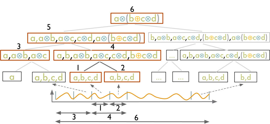
Figure 4. Bottom-up scoring of ShapeQuery

Figure 4 depicts the logical order for scoring ShapeQuery a$\color[rgb]{0,.5,.5}\otimes$(b$\color[rgb]{1,.5,0}\oplus$(c$\color[rgb]{0,.5,.5}\otimes$d)) over the sub-sub-regions. Here, a, b, c, and d represent a ShapeSegment. The SegmentTree algorithm starts by scoring individual ShapeSegments (e.g., a,b,c and d in a$\color[rgb]{0,.5,.5}\otimes$(b$\color[rgb]{1,.5,0}\oplus$(c$\color[rgb]{0,.5,.5}\otimes$d))) independently over each of leaf nodes as depicted in Figure 4. Next, it computes the scores of sub-sequences in the intermediate nodes using the merging process described below. For example, in Figure 4, node 4 depicts the sub-sequences formed by combining sub-sequences from nodes $1$ and $2$, and node 5 depicts the sub-sequences formed by combining sub-sequences from nodes $3$ and $4$. When multiple sub-sequences in the children nodes generate the same sub-sequence in the parent node, we select the sub-sequences that result in maximum score after concatenation (i.e., the one with the best optimal segmentation), thereby pruning out LOPs corresponding to non-selected sub-sequences. For example, at node 5, a$\color[rgb]{0,.5,.5}\otimes$b can be computed from 1) a from node $3$ and b from node $4$, 2) a$\color[rgb]{0,.5,.5}\otimes$b from node $3$ and b from node $4$, and 3) a from node $3$ and a$\color[rgb]{0,.5,.5}\otimes$b from node $4$. Among the 3 concatenations, we pick the one that gives the maximum score.

Algorithm 2 Fuzzy Matching Algorithm

Input: $L$: a sub-region of trendline, $Q$: a CONCAT operation, $ScrFunc$: scoring functions from Tables 4 and  4

Output: score

1:procedure ExecFuzzyQuery($L$, $Q$, $ScrFunc$)

2:    $subRegions$ $\leftarrow$ $ComputeSubRegions(L)$ // leaf nodes

3:    $T$ $\leftarrow$ $ComputeSubSequences(Q)$

4:    $nodes$ $\leftarrow$ Queue()

5:    // scoring of leaf segments

6:    for each $s$ in $subRegions$ do

7:         $lops$ $\leftarrow$ []

8:         for each $t$ in $T$ do

9:             $lops$[$t$] $\leftarrow$ SelectLOPs($s$,$t$)

10:         end for

11:         $node$ $\leftarrow$ [$s$.start, $s$.end, lops[$t$]]

12:         $nodes$.add(node)

13:    end for

14:    // bottom-up processing

15:    while $nodes$.size() ¿ 1 do

16:         $s$ $\leftarrow$ $nodes$.Size()

17:         // pairwise merging of nodes at the same level

18:         while $s$ ¿ 0 do

19:             $s1$ $\leftarrow$ $nodes$.deque(), $s2$ $\leftarrow$ $nodes$.deque()

20:             $mlops$ $\leftarrow$ []

21:             for each $t1$,$t2$ in $s1$.$lops$.keys(),$s2$.$lops$.keys() do

22:                 $score$, $lops$ $\leftarrow$ Merge($L$, $s1$[$t1$],$s2$[$t2$])

23:                 if $score$ $>$ $mlops$[$t1$$\color[rgb]{0,.5,.5}\otimes$$t2$].score then

24:                     $mlops$[$t1$$\color[rgb]{0,.5,.5}\otimes$$t2$ ] = {$lops$, $score$}

25:                 end if

26:             end for

27:             $node$ $\leftarrow$ [$s1$.start, $s2$.end, $mlops$]

28:             $nodes$.add(node)

29:             $s$ = $s$ $-$ $1$;

30:         end while

31:    end whilenode $\leftarrow$ $nodes$.deque()

32:    return $node$.$lops$[$Q$].$score$

33:end procedure

Theorem 3.2.

Given the closure assumption, the bottom-up algorithm with $k$ CONCAT operands is optimal with a time complexity of $O(nk^{4})$, i.e., linear in the number of points in the trendlines.

Proof: We prove the above theorem via induction.

Base case. For a single node SegmentTree, there is no difference between the SegmentTree algorithm and DP, since the SegmentTree algorithm uses DP to select the LOPs for a single node.

Induction step. Let $L$ and $R$ be two sibling nodes in the SegmentTree consisting of optimal scores for each possible subsequence of operands in the CONCAT operations, and let $P$ be their parent node. Let $S^{L}_{i(k-1)}$ be the score of sub-expression from operand $i$ until $k$ in $L$ for the optimal segmentation of $(i-1)$th to $k$th operands in L and $S^{R}_{(k+1)j}$ be the score of the sub-expression from operand $k+1$ until $j$ for the optimal segmentation of $k$th to $j+1$th operands in $R$. Let $S^{P}_{ij}$ be the score of sub-expression of operand $i$ until $j$ in $P$, formed by concatenation of operands $i-1$ until $k$ in $L$ and $k$ until $j+1$ in $R$. As per the Closure assumption, the optimal segmentation corresponding to $S^{P}_{ij}$ must include the optimal segmentation $i-1$ until $k$ in $L$ and $k$ until $j+1$ in $R$. Since $kth$ operand is common between $L$ and $R$, we need to re-compute its score over the sub-region from x.e of $(k-1)$th operand in $L$ and x.s of $(k+1)$th operand in $R$ during concatenation. Let $sc^{P}_{k}$ be the re-computed score of the $k$th ShapeSegment. Then, $S_{ij}$ can thus be computed as:

$S_{ij}$ $=\underset{k}{MAX}\{\frac{(k-i)\times S^{L}_{i(k-1)})+sc^{P}_{k}+(j-k)\times S^{R}_{(k+1,j)})}{(j-i+1)}\}$

Since, for computing $S_{ij}$, we consider all possible combinations of optimal segmentations in $L$ and $R$ and pick the one that gives the maximum score, it must be optimal.

Conclusion. Thus, by the principle of induction, the SegmentTree algorithm must also be optimal over the entire SegmentTree.

Time Complexity. For a sub-region of $n$ points, the maximum number of leaf nodes is $n/2$ (since we need at least 2 points per sub-region) and therefore the total number of nodes in the tree is $n$. At each of the leaf node, we estimate the scores of each ShapeSegment independently, taking $O(n\times k)$ operations across all leaf nodes. Each intermediate node involves a merge step, involving concatenation of subsequences from left node with the right node. For $k$ operands in CONCAT, there can be a maximum of $k^{2}$ subsequences per node, requiring a total of $k^{4}$ concatenations. Moreover, each concatenation involves the computation of score $sc^{P}_{k}$ of the $k$th ShapeSegment that intersects left and right child. The computation of $sc^{P}_{k}$ involves the estimation of the slope of line from x.e of $(k-1)$th ShapeSegment in $L$ to x.s of $k+1$th ShapeSegment in $R$, which can be done in constant time from the statistics of $k$th ShapeSegment’s sub-region in $L$ and $R$ (see Theorem 3.3). Thus, each merging step involves $O(k^{4})$ operations. Overall, the SegmentTree algorithm takes $O(n/2\times k^{4}+nk)$ $\approx$ $O(nk^{4})$ time, i.e., linear in the number of points in the sub-region. In practice, $k^{4}$ is not a problem, since not all combinations of sub-sequences lead to a valid sub-sequence in the CONCAT operands, therefore the actual number of merges are much fewer. Moreover, $k$ is typically small ($\leq 5$). $\square$.

3.3. Pruning Optimization

A large number of ShapeQueries are sequential pattern matching queries, consisting of only a single CONCAT operation on a sequence of simple patterns such as up, down, $\color[rgb]{0.5,0.5,0}\theta=x$. For such CONCAT operations, we can bound the final scores of trendlines and filter low-scoring trendlines without scoring them until the root node of the SegmentTree. We first describe our key observations.

Observation 3.1 Given a sub-region $L$ comprising of sub-sub-regions: $L_{1},L_{2},...,L_{n}$, the score of a ShapeSegment consisting of patterns up or down over L, $score_{up/down,L}$ is bounded between the maximum and minimum scores over any of the smaller sub-regions, i.e., $\underset{i}{MIN}(score_{up/down,L_{i}})$ $\leq$
$score_{up/down,L}$ $\leq$ $\underset{i}{MAX}(score_{up/down,L_{i}})$.

This observation holds because the scores of up or down vary monotonically with the slope of the line, and the slope of the line over the large sub-region is always bounded between the maximum and minimum slopes of the lines over any smaller regions, $\underset{i}{MIN}(slope_{L_{i}})$ $\leq$
$slope_{L}$ $\leq$ $\underset{i}{MAX}(slope_{L_{i}})$

However, when a slope (e.g., $\color[rgb]{0.5,0.5,0}\theta=x$) is specified as pattern, the above observation does not hold for $\underset{i}{MIN}(slope_{L_{i}})$ $\leq$ $x$ $\leq$ $\underset{i}{MAX}(slope_{L_{i}})$, because the $score_{x,L}$ can be more than $\underset{i}{MAX}(score_{x,L_{i}})$ when $|x-slope_{L}|\leq\underset{i}{MIN}(x-slope_{L_{i}})$. For such cases, we set the upper bound to $1$, the maximum possible score.

Observation 3.2 The score of an operator is bounded between the minimum and maximum scores of input ShapeSegments.

This observation is clear from the scoring functions of operators as defined in Table 4.

Based on the above observations, we can derive the bounds on the final score of a ShapeSegment at the root node using the maximum and minimum scores of the ShapeSegment at a given level $i$ in the SegmentTree. We summarize the bounds for each of the patterns in Table  5.

Thus, instead of processing each trendline completely in one go, we process trendlines in rounds. In each round, we process one level of SegmentTree for all of the trendlines simultaneously, and incrementally refine the upper and lower bounds on their scores. Before moving on to the upper levels, we prune the trendlines that have their upper bound score lower than the current top-$k$ lower bound scores. Overall, the pruning optimization helps avoid processing to completion for a large number of trendlines in the collection, and is particularly effective when the user is looking for trendlines with rare patterns.

Table 5. Bounds on scores for different patterns based on scores at a given level $i$ in the SegmentTree

Pattern	Max possible Score	Min possible Score
up	max across all level $i$ nodes	min across all level $i$ nodes
down	max across all level $i$ nodes	min across all level $i$ nodes
flat	3cmmax across all level $i$ nodes if all $\theta$ ¿ 0 or all $\theta$ ¡ 0; otherwise 1	min across all level $i$ nodes
$\theta=x$	3cmmax across all level $i$ nodes if all $\theta$ ¿ $x$ or $\theta$ ¡ $x$ ; otherwise 1	min across all level $i$ nodes

Table 6. NL Features. d(x) denotes the number of words between current word and x, x+ and x- denote next and previous x

Type	Features
POS Tags	pos-tag, pos-tag-, pos-tag+
Words	word-, word+, word–, word++
synonym	synonym, synonym+, synonym-, d(synonym+), d(synonym-)
Space and time prepositions	time-preposition+, time-preposition-, space-preposition+, space-preposition-, d(time-preposition+), d(time-preposition-), d(space-preposition+), d(space-preposition-)
Punctuation	d(,+), d(,-) ,d(;+), d(;-), d(.+), d(.-)
Conjunctions	d(and+), d(or-), d(and then+)
Miscellaneous	d($x$), d($y$), d(next), ends(ing), ends(ly), length(query)

Table 7. Common Ambiguities and their Resolution

Ambiguity (example queries with predicted entities)	Rules for Resolution
A1: Conflicting LOCATION and PATTERN in a ShapeSegment (e.g., [decreasing ($p$) from $4$ ($x.s$) to $8$ ($x.e$)])	R1: Change the sub-primitive of LOCATION from $x$ to $y$ or $y$ to $x$. R2: Swap the start and end positions of LOCATION.
A2: Multiple $p$ in the same ShapeSegment (e.g., [increasing ($p$) from $2$ ($x.s$) to $5$ ($x.e$) with decreasing ($p$)] next ($\color[rgb]{0,.5,.5}\otimes$))	R1: Move one of the $p$s to the adjacent ShapeSegment with missing $p$. R2: split the ShapeSegment into two new ShapeSegments with an OR operator between them
A3: Overlapping ShapeSegments with $\color[rgb]{0,.5,.5}\otimes$(e.g., increasing ($p$) from $4$ ($x.s$) to $8$ ($x.e$) and then ($\color[rgb]{0,.5,.5}\otimes$) decreasing ($p$) from $8$ ($x.s$) to $0$ ($x.e$)	R1: Change $x$ to $y$, if $y$ values missing. If $y$ values already present, replace $\color[rgb]{0,.5,.5}\otimes$ with $\color[rgb]{.75,.5,.25}\odot$ operator.

3.4. Additional Optimizations

ShapeSearch supports a couple of additional optimizations that result in faster scoring of trendlines.

Generating lines via Summary Statistics. For scoring a sub-region, ShapeSearch fits a line to approximate it. This is costly for fuzzy ShapeQueries where ShapeSearch needs to score sub-regions of varying sizes, fitting one line for every sub-region. We note that a summary of five statistics namely, $\sum x_{i}$, $y_{i}$, $\sum x_{i}.y_{i}$, $\sum x_{i}^{2}$, and $n$ for a sub-region, is sufficient to compute the slope of the line over the sub-region as follows: $\theta$=$\frac{(n\times\sum x_{i}.y_{i}-\sum x_{i}\sum y_{i})}{(n\times\sum x_{i}^{2}-(\sum x_{i})^{2})}$, $\delta$=$\sum y_{i}-\theta\times\sum x_{i}$.
Moreover, it is easy to see that the individual summaries over two sub-regions ($A$ and $B$) are sufficient to compute the slope of the line over the combined region $AB$, without making additional passes over the data.

$\theta_{AB}$= $\frac{(n_{A}+n_{B})*(\sum x_{Ai}.y_{Ai}+\sum x_{Bi}.y_{Bi})-(\sum x_{Ai}+\sum x_{Bi})*(\sum y_{Ai}+\sum y_{Bi})}{(n_{A}+n_{B})\times\sum((x_{Ai})^{2}+(x_{Bi})^{2})-\sum(x_{Ai}+x_{Bi})^{2}}$

Thus, the summary statistics help reduce data movement as well as the amount of data processed during segmentation. We summarize our finding using the following theorem.

Theorem 3.3 (Additivity).

Given two adjacent segments A and B, a line segment over the combined segment AB can be estimated using linear regression on the summarized statistics over the individual segments A and B.

Push-Down Optimizations. ShapeSearch applies a number of push-down optimizations when a ShapeQuery involves location constraints. Consider a ShapeQuery: [ p= up,x.s=50, x.e=100][ p=down][ p=up] that searches for shapes which are $increasing$ from $50$ to $100$ followed by a decreasing, and then an $increasing$ pattern. ShapeSearch employs three push-down optimizations for such queries: (1) LOCATION primitives in ShapeQuery are pushed down to the trendline generation component to prune trendlines that do not have any value in the specified $x$ ranges (e.g., $50$ to $100$ in the above query), (2) When a ShapeQuery contains a ShapeSegment with an p=up or p=down pattern along with both start and end locations (e.g., [ p=up, x.s=50,x.e=100] in the above query), ShapeSearch prioritizes the segmentation of ShapeSegments over such location primitives first, since the trendlines with negative scores over such sub-regions tend to have substantially lower scores. This helps the pruning of low scoring trendlines much earlier in the SegmentTree, and (3) Finally, ShapeSearch avoids computing summary statistics over $x$ ranges that are not used in the ShapeQuery (e.g., $0$ to $50$ in the above query), since the values over such ranges are ignored for segmentation and scoring. Overall, as we will see in Section 5, these push-down optimizations significantly help in improving the overall response time of the ShapeSearch.

4. Natural Language Translation

So far, we haven’t described how natural language queries are parsed into ShapeQueries.

We now provide a brief overview of the key steps involved in parsing. We use the following natural language query collected from MTurk for illustration: “show me the trendlines that are increasing from $2$ to $5$ and then decreasing”

Step 1. Primitives and Operators Recognition. Given a natural language query, the first step is to map words to their corresponding shape primitives and operators. We follow a two-step process. First, using the Part-of-Speech (POS) tags and word-level features, we classify each word in the query as either noise or non-noise. For example, words $\in$ {determiner, preposition  stop-words} are more likely to be noise, while words $\in$ {noun, adjective, adverb, number, transition words, conjunction} may refer to a primitive or operators. Next, given a sequence of non-noise words, we use a linear-chain conditional-random field model (CRF) (lafferty2001conditional, ) (a probabilistic graphical model used for modeling sequential data, e.g., POS tagging) to predict their corresponding primitives and operator. For example, the above query is tagged as “show (noise) me (noise) the (noise) trendlines (noise) that (noise) are (noise) increasing ( p) from (noise) $2$ ( x.s) to (noise) $5$ ( x.e) and then ($\color[rgb]{0,.5,.5}\otimes$) decreasing ( p)”..

We train the CRF model (lafferty2001conditional, ) on the same $250$ natural language queries that we used for characterizing trendline patterns (Section 1). We provide more details on how we collected the queries in Appendix A.1. We extract a set of features (listed in Table 7) for each non-noise word in the sequence. In addition, ShapeSearch stores “synonyms” for each primitve and operator (e.g., “increasing” for up, “next” for CONCAT), and if a non-noise words closely matches with them (e.g., with edit distance $<=2$), we add the matched primitive or operator as a feature called predicted-entity. This idea is inspired from the concept of “boostrapping” in weakly-supervised learning approaches (kozareva2011class, ; siddiqui2016facetgist, ), and helps improve the overall accuracy. We implemented the model using the Python CRF-Suite library  (pythoncrfsuite, ) with parameter settings: L1 penalty:1.0, L2 penalty:0.001, max iterations: 50, feature.possible-transitions: True. On $5$-fold cross-validation over the crowd-sourced queries, the model had an $F1$ score of $81\%$ ($precison=73\%$, $recall=90\%$).

Step 2. Identifying Pattern Value. For each of the words predicted of type p, e.g., increasing and decreasing in the above query, we additionally map them to the corresponding semantic pattern supported in ShapeSearch, e.g., “increasing” is mapped to p=up. For this mapping, ShapeSearch computes the similarity between the specified word and synonyms of the supported patterns, first using edit distance and then using wordnet (roetter2005integration, ). The semantic pattern with the highest similarity between any of its synonyms and the specified word is selected.

Step 3. ShapeQuery Generation and Ambiguity Resolution. Next, we group primitives and operators into a ShapeQuery. ShapeSearch first groups all the primitives between two operators into a single ShapeSegment. For instance, for the above query, the primitives are grouped as follows: [increasing ( p=up), $2$ ( x.s), $5$ ( x.e) ] and then ($\color[rgb]{0,.5,.5}\otimes$) [ decreasing ( p=down)]. In some cases, this may lead to incorrect grouping of primitives, e.g., two patterns in the same ShapeSegment. Moreover, there could be semantic ambiguity because of incorrect entity tagging, e.g., decreasing ( p=up) from $5$ ( y.s) to $10$ ( y.e) where x.s and x.e values are wrongly tagged as y.s and y.e respectively. ShapeSearch uses rule-based transformations that try to reorder and change the types of entities to get a correct and meaningful ShapeQuery. In Table 7, we list three common ambiguities (A1, A2, A3) and a sequence of rules (e.g., R1, R2) that are applied in order to resolve these.

The parsed ShapeQuery is sent to the front-end, and displayed as part of the correction panel (Box 4 in Figure 2(a)) for users to edit or further refine the parsed representation if needed. The validated query is then executed to generate the matching trendlines.

					Runtime (sec)						Accuracy (%)
	Dataset	—V—	$|V_{i}|$	Query	Exhuastive	DP	DTW	Segment Tree	Segment Tree+Prune	Greedy	Segment Tree	Greedy
1	Weather	144	366	( ${\theta}{=}45^{\circ}$$\color[rgb]{0,.5,.5}\otimes$ d$\color[rgb]{0,.5,.5}\otimes$ u$\color[rgb]{0,.5,.5}\otimes$ d)	290	52	11	5	2.8	0.9	85	25
2	Weather	144	366	(( u$\color[rgb]{1,.5,0}\oplus$ d)$\color[rgb]{0,.5,.5}\otimes$ f$\color[rgb]{0,.5,.5}\otimes$ u$\color[rgb]{0,.5,.5}\otimes$ d)	211	55	9	4	3.2	1.1	90	30
3	Weather	144	366	( f$\color[rgb]{0,.5,.5}\otimes$ u$\color[rgb]{0,.5,.5}\otimes$ d$\color[rgb]{0,.5,.5}\otimes$ f )	244	47	9	5	3.3	1.4	100	25
4	Worms	258	900	( d$\color[rgb]{0,.5,.5}\otimes$( ${\theta}{=}45^{\circ}$ $\color[rgb]{1,.5,0}\oplus$ ${\theta}{=}{-}20^{\circ}$ )$\color[rgb]{0,.5,.5}\otimes$ f)	4737	76	53	10	7	2.2	90	35
5	Worms	258	900	( d$\color[rgb]{0,.5,.5}\otimes$ ${\theta}{=}45^{\circ}$$\color[rgb]{0,.5,.5}\otimes$ d)	4320	63	44	12	9	3.4	90	35
6	Worms	258	900	( u$\color[rgb]{0,.5,.5}\otimes$ d$\color[rgb]{0,.5,.5}\otimes$ u)	3953	68	42	9	6	2.5	90	20
7	50Words	905	270	( d$\color[rgb]{0,.5,.5}\otimes$( u$\color[rgb]{1,.5,0}\oplus$( f$\color[rgb]{0,.5,.5}\otimes$ d)))	1046	105	28	7	5	1.1	90	25
8	50Words	905	270	( d$\color[rgb]{0,.5,.5}\otimes$ ${\theta}{=}45^{\circ}$$\color[rgb]{0,.5,.5}\otimes$ d)	954	122	32	7	5	1.9	100	40
9	50Words	905	270	(( u$\color[rgb]{1,.5,0}\oplus$ d)$\color[rgb]{0,.5,.5}\otimes$( u$\color[rgb]{1,.5,0}\oplus$ d)$\color[rgb]{0,.5,.5}\otimes$ f)	979	131	29	9	7	1.2	85	40
10	Housing	1777	138	( f$\color[rgb]{0,.5,.5}\otimes$ d$\color[rgb]{0,.5,.5}\otimes$ u$\color[rgb]{0,.5,.5}\otimes$ f)	165	58	40	14	12	1.5	80	15
11	Housing	1777	138	( u$\color[rgb]{0,.5,.5}\otimes$ d$\color[rgb]{0,.5,.5}\otimes$ u$\color[rgb]{0,.5,.5}\otimes$ f)	152	63	41	17	13	1.9	85	20
12	Housing	1777	138	( u$\color[rgb]{0,.5,.5}\otimes$ f$\color[rgb]{0,.5,.5}\otimes$(( ${\theta}{=}45^{\circ}$$\color[rgb]{0,.5,.5}\otimes$ ${\theta}{=}60^{\circ}$)$\color[rgb]{1,.5,0}\oplus$( u$\color[rgb]{0,.5,.5}\otimes$ d)))	157	52	35	18	14	1.2	75	15
13	Haptics	463	1092	( u$\color[rgb]{0,.5,.5}\otimes$ d$\color[rgb]{0,.5,.5}\otimes$ f$\color[rgb]{0,.5,.5}\otimes$ u)	6869	890	62	16	12	3.1	90	40
14	Haptics	463	1092	( d$\color[rgb]{0,.5,.5}\otimes$ u$\color[rgb]{0,.5,.5}\otimes$ d$\color[rgb]{0,.5,.5}\otimes$ f)	7189	924	58	20	15	2.6	95	25

Figure 5. Runtime and accuracy results

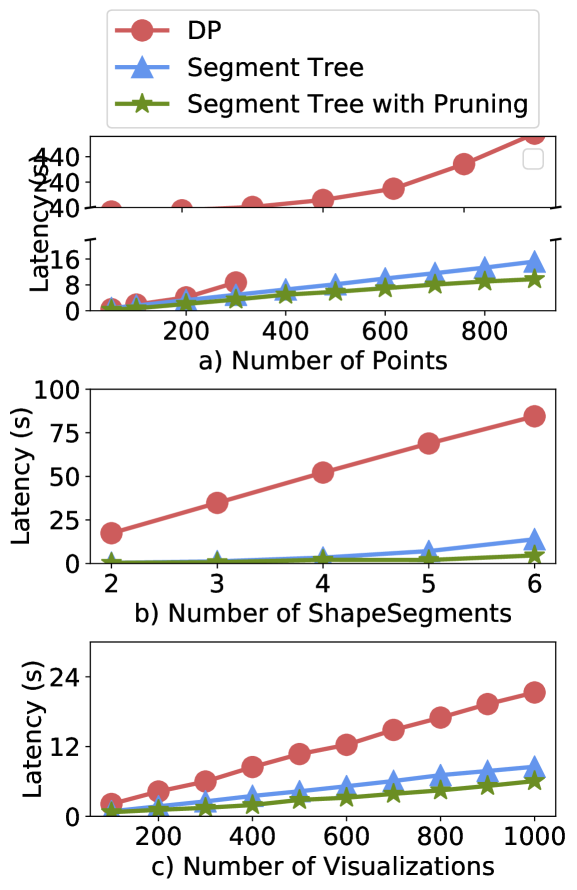
Figure 6. Impact on varying characteristics of ShapeQueries

5. Performance Evaluation

In this section, we evaluate the runtime and accuracy of ShapeSearch pattern matching algorithms. We first compare the runtime of the exhaustive pattern matching algorithm (Section 2.3) with four algorithms proposed in Section 3: (i) the dynamic programming-based (DP) algorithm, (ii) the Greedy algorithm, (iii) the SegmentTree algorithm, and (iv) the SegmentTree algorithm with pruning. We also compare with Dynamic Time Warping (DTW) (dtw, ), another dynamic-programming algorithm that is typically used for matching shapes in trendlines in systems like Zenvisage (zenvisagevldb, ), to show the efficiency of ShapeSearch relative to existing systems. Next, we compare the accuracy of SegmentTree and Greedy with respect to the results of DP. Note that SegmentTree and Greedy are approximate while DP is an optimal algorithm and gives the same results as that of the exhaustive algorithm. Finally, we vary the characteristics of ShapeQueries to assess the impact of different factors on performance.

Datasets and Setup. Figure 6 depicts the five real-world datasets drawn from the UCI repository (ucirepo, ), and the list of queries we used for our experiments. Each dataset consists of trendlines with a mix of shapes, and the datasets differ from each other in terms of number of trendlines ($|V|$) as well as their length ($|V_{i}|$). The queries were selected to have at least $20$ trendlines with scores $>0$ to ensure that the issued ShapeQueries were relevant to the dataset. All experiments were conducted on a 64-bit Linux server with 16 2.40GHz Intel Xeon E5-2630 v3 8-core processors and 128GB of 1600 MHz DDR3 main memory. Datasets were stored in memory, and we ran six trials for each query on each dataset.

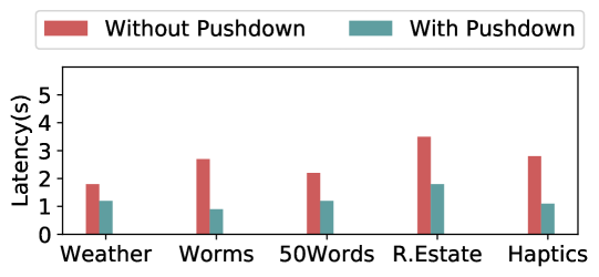
Figure 7. Average running time before and after push-down optimizations on non-fuzzy queries.

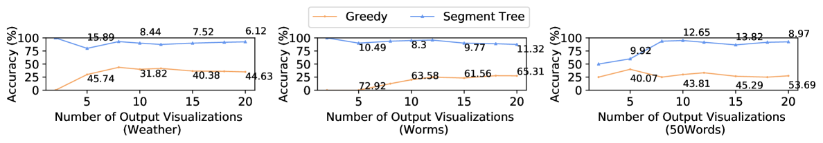
Figure 8. Accuracy with respect to DP over $3$ real datasets with varying number of output trendlines. Annotations denote the average deviation (in %) of the score of $kth$ trendline chosen by algorithms with respect to the $kth$ optimal trendline.

5.1. Overall Run-time and Accuracy

Runtime Comparison. Figure 6 (Runtime) depicts the runtime for each of the queries across all datasets. We see the time taken by the exhaustive algorithm is prohibitively large, rendering it no longer interactive. DP provides an order of magnitude speed-up over the exhaustive approach; however even DP can take $100$s of seconds over trendlines with only a few hundred points. Both Greedy and SegmentTree provide a $2\times$ to $40\times$ improvement in runtime compared to DP, taking only a few seconds in the worst case. These algorithms explore a much fewer number of segmentations compared to the DP approach. We also see that these algorithms are about $10\times$ faster than the DTW algorithm, whose runtime, like DP, varies quadratically with the number of points in the trendline. Finally, SegmentTree with Pruning further provides a speed-up of 10-30% by pruning low utility trendlines. Since the improvement in performance of SegmentTree and Greedy comes at the cost of accuracy, we next compare the accuracies.

Acccuracy Comparison. Figure 6 (Accuracy) depicts the accuracy of SegmentTree and Greedy relative to DP. We do not compare the accuracy of DTW with ShapeSearch algorithms since their scoring functions differ; instead we perform an user study in the next section to compare the effectiveness of ShapeSearch scoring functions with DTW and other similar metrics. We define accuracy here to be the number of trendlines picked by the algorithm that are also present in the top $20$ trendlines selected by DP. We see that Greedy has a low accuracy ($<30\%$), since it gets stuck at local optima. The accuracy of SegmentTree is closer to that of DP and is never off by more than $2$ trendlines when we look at top 10 visualizations. Unlike Greedy, SegmentTree compares the local patterns in the trendlines and those specified in the ShapeQuery to select the segmentations that could result in high score.

Figure 8 depicts the accuracy results over top-$k$ visualizations (with $k$ varying from $2$ to $20$) for 3 of the the datasets. Annotations in each of the figures depict the average deviation in % of the score of $kth$ visualization that an algorithm selects with respect to the score of the $kth$ optimal visualization, indicating how off the shapes of selected visualizations are from optimal ones. We note that the accuracy of SegmentTree improves as the number of output visualizations increases, and is never off by more than $2$ visualizations or have more than $>12\%$ deviation in scores when we look at top $20$ visualizations.

Overall, the runtime and accuracy results demonstrate that the SegmentTree achieves comparable accuracy to that of DP in much less time.

Next, we explore the impact of push-down optimizations, discussed in Section 3.4, on the overall performance of queries.

Impact of Push-Down Optimizations. We issue non-fuzzy queries, one query for each of the datasets, as depicted in Table 8. Figure 7 depicts the runtimes for ShapeSearch (note that all ShapeSearch algorithms behave similarly for non-fuzzy queries) with and without push-down optimizations. We observe that non-fuzzy queries execute very quickly ($<4s$ for over $1000$ trendlines with more than $1000$ points each), but pushdown optimizations help in further reduction of runtime in proportion to the selectivity of the LOCATION primitives in the query. For example, for ShapeQuery [ p=up, x.s=60,x.e=80] on the Haptics dataset, pushdown optimizations help reduce the runtime from $3s$ to $<1.2s$.

Table 8. Non-Fuzzy Queries

Name	Non-Fuzzy Queries
Weather	[p=down,x.s=1,x.e=4]$\color[rgb]{0,.5,.5}\otimes$[p=up,x.s=4,x.e=10]$\color[rgb]{0,.5,.5}\otimes$[ p=down, x.s=10,x.e=12]
Worms	[ p=down, x.s=50,x.e=100]
50 Words	[ p=down, x.s=200,x.e=400]$\color[rgb]{0,.5,.5}\otimes$[ p=up, x.s=800,x.e=850]
Real Estate	[ p=down, x.s=1,x.e=20]$\color[rgb]{0,.5,.5}\otimes$[ p=up, x.s=20,x.e=60] $\color[rgb]{0,.5,.5}\otimes$[ p=down, x.s=60,x.e=138]
Haptics	[ p=up, x.s=60,x.e=80]

5.2. Varying ShapeQuery Characteristics

We evaluated the efficacy of our SegmentTree-based optimizations with respect to three different characteristics of ShapeQueries, as discussed below.

Impact of number of data points. Figure 6 shows the performance of algorithms as we increase the number of data points in trendlines for a fuzzy ShapeQuery (u$\color[rgb]{0,.5,.5}\otimes$d$\color[rgb]{0,.5,.5}\otimes$u $\color[rgb]{0,.5,.5}\otimes$d). With the increase in data points, the overall runtimes increases for all algorithms because of the increase in the number of segmentations. Nevertheless, SegmentTree shows better performance than DP after 100 data points since the SegmentTree approach is less sensitive (linear time) to the number of data points than that of DP (quadratic).

Impact of number of patterns. Figure 6 depicts the performance of fuzzy ShapeQueries with varying the number of ShapeSegments (alternating $up$ and $down$ patterns) and issued over the weather dataset. As the number of ShapeSegments in the ShapeQuery grows, the overall runtimes of the algorithms also increases, with the runtimes for SegmentTree and SegmentTree with pruning growing much faster ($k^{4}$) than DP ($k$). However, the overall time for DP is still larger because the number of data points ($366$ in the weather dataset) plays a more dominant ($n^{2}$) role.

Impact of number of trendlines. We increased the number of trendlines from $100$ to $1000$ in the real-estate dataset with a step size of 100 and issued a fuzzy ShapeQuery ($u$$\color[rgb]{0,.5,.5}\otimes$$d$ $\color[rgb]{0,.5,.5}\otimes$$u$$\color[rgb]{0,.5,.5}\otimes$$d$); the results are depicted in Figure 6. While the overall runtime for all approaches grows linearly with the number of trendlines, the gap between SegmentTree and SegmentTree with pruning grows wider. This is because more trendlines get pruned as the size of the collection grows larger.

6. User Study

We conducted a user study to perform a qualitative and quantitative comparison of ShapeSearch with two baseline tools: our prior work Zenvisage (zenvisagevldb, ) and Qetch (qetchchi, ), two recent sketch-based systems for trendline pattern search (depicted in Figure 9). These systems allow users to sketch a pattern on a canvas, zoom in and out of the trendline to focus on a specific sub-region, and apply filtering and smoothing to match trendlines at varying granularities. While Qetch supports its own custom shape matching algorithm, Zenvisage allows users to choose between the Euclidean or DTW distance measures depending on the task. Qetch additionally supports a simple regex (via a repeat operator) to search for repeated occurrences of a sketched pattern. We disabled the sketching capability in ShapeSearch to isolate the benefits of the novel NL and regex query mechanisms over sketch. ShapeSearch^∗ denotes ShapeSearch with only NL- and regex-based querying mechanisms. We recruited 24 (14M/10F) participants with varying degrees of expertise in data analytics via flyers and mass-emails. We employed within-subjects study design between ShapeSearch^∗ and each of the baseline tools, using two groups of 12 participants each. Note that by design, each participant encountered sketch capabilities only once—either in Zenvisage or Qetch. Participants were free to employ either NL or Regex for ShapeSearch^∗.

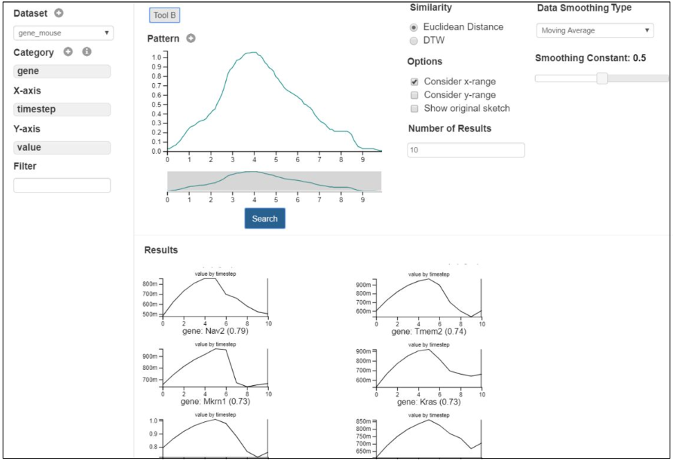
(a) Zenvisage

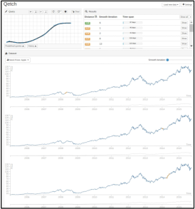
(b) Qetch

Figure 9. Baseline interfaces for user study

Dataset and Tasks. Based on the domain case studies from Section 1, as well as prior work in time series data mining (ralanamahatana2005mining, ; ye2009time, ; fu2011review, ; olszewski2001generalized, ; han2011data, ) and visualization (2017-regression-by-eye, ; correll2016semantics, ; zenvisagevldb, ; timesearcher, ; googlecorrelate, ), we identified seven categories of pattern matching tasks, as depicted in Table 9. We designed these tasks on two real-world datasets: the Weather and the Dow Jones stock datasets from the UCI repository (ucirepo, ) that participants could easily understand and relate with. Together, the seven tasks spanned both exploratory search as well as targeted pattern-based data exploration, which helped us test the effectiveness of individual interfaces in various settings.

Ground Truth.

For selecting the ground truth, three of the authors independently assigned a score in a range of $5$ (best match) to $0$ (worst match) for each of the trendlines, and filtered out trendlines with average score $<$ 3.0. Next, we leveraged $20$ mturk workers per task to rate each selected trendline in a range of 0-3 (later scaled to $3-5$). Each mturk worker was presented with the task description in Table 9, along with a collection of trendlines, each of which they had to rate based on how closely the trendline matched the task description. Filtering out noisy trendlines in the first step helped minimize the number of ratings per task, thereby improving the effectiveness of workers. Finally, we take the average of the scores given by three authors and workers as the ground truth score for a trendline. For a given task, we measure the task-accuracy as (sum of the ground truth scores of the top-K trendlines selected by the participant) $\times$ 100 / (sum of the top-K ground-truth scores for the task). $K$ varied between $2$ to $5$ per task.

6.1. Key Findings

Table 9. Pattern Matching Tasks

Tasks	Description
Exact Trend Match (ET)	Find shapes similar to a specific shape, e.g., cities with weather patterns similar to that of NY, stock trends similar to Google’s.
Sequence Match (SQ)	Find shapes with similar trend changes over time, e.g., cities with the following temperature trends over time: rise, flat, and fall, stocks with decreasing and then rising trends.
Common Trends ( TC)	Summarizing common trends e.g., find cities with typical weather patterns, stock with typical price patterns.
Sub-pattern Match (SP)	Find frequently occurring sub-pattern, e.g., stocks that depicted a common sub-pattern found in stocks of Google and Microsoft, cities with $2$ peaks in temperature over the year.
Width specific Match (WS)	Find shapes occurring over a specific window, e.g., cities with steepest rise or fall in temperature over $3$ months, peaks with a width of $4$ months.
Multiple X or Y constraints (MXY)	Find shapes with patterns over multiple disjoint regions of the trendline, e.g., stocks with prices rising in a range of 30 to 60 in march, then falling in the same range over the next month.
Complex Shape Matching (CS)	Find shapes involving trends along specific directions, and occurring over varying duration, e.g., stocks with head and shoulder pattern, cup-shaped patterns, W-shaped patterns.

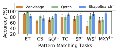
(a) Task Accuracy

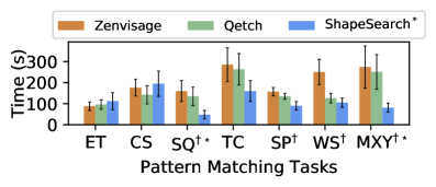
(b) Task Completion Time

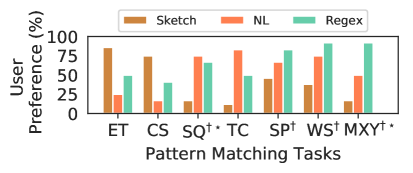
(c) User Preferences

Figure 10. User study results ($\dagger$ and $\ast$ denote that ShapeSearch^∗ had statistically significant improvements ($\alpha$ = 5%) relative to Zenvisage and Qetch respectively

We describe our key findings below.

Overall Task Accuracy and Completion Times. As depicted in Figure 10(a) and Figure 10(b), ShapeSearch^∗ helped participants achieve higher accuracy and less time overall than Qetch and Zenvisage, and in particular for, $5$ out of $7$ tasks; however, for precise and complex shape matching tasks, ShapeSearch^∗ performed worse than baselines due to the lack of sketch capabilities. On average across all tasks, ShapeSearch^∗ helped participants achieve an accuracy of 87%—8% more than Qetch and 17% more than Zenvisage—in about 30-40% less time, a significant improvement. While Zenvisage and Qetch involve less reasoning during query synthesis, they often lead to significantly more queries issued and manual browsing of trendlines for identifying the desired ones. ShapeSearch^∗, on the other hand, can accept more fine-grained user queries to rank relevant trendlines effectively, enabling participants to retrieve more accurate answers with less effort. In order to better understand the differences between the tools, we separately analyze tasks where ShapeSearch^∗ did better and worse than the baselines.

Settings Where ShapeSearch^∗ Wins. Since sketch systems are based on precise matching, for sequence and sub-pattern matching tasks (SQ and SP), users drew multiple sketches for a given sequence or subsequence to find all possible instances. ShapeSearch^∗, however, is effective at automatically considering a variety of shapes that satisfy the same sequence or subsequence of patterns. Similarly, for tasks involving multiple constraints along the X and Y axes, or the width of patterns (TC, WS, MXY), a large majority of the participants gave more accurate results in less time with ShapeSearch^∗. ShapeSearch^∗ supports a rich set of primitives for users to add multiple constraints to the patterns, including searching for patterns over multiple disjoint regions. While the users could zoom into a specific region of the trendline and sketch their desired patterns in the sketch systems, these capabilities were not sufficient to precisely specify all of the constraints at the same time. We believe that supporting visual widgets in the baseline tools that internally leverages the ShapeSearch primitives could remedy this issue.

Settings Where ShapeSearch^∗ Loses. The opposite effect was observed (more time, less accurate with ShapeSearch^∗) when finding trendlines exactly similar to a given trendline (ET). This is understandable given that ShapeSearch^∗ does not possess sketching capabilities, which is a perfect fit for this task, and that ShapeSearch^∗ regex scoring functions are targeted more towards approximate and fuzzy pattern matching. For complex shapes (CS), Qetch performed the best, followed by ShapeSearch^∗, and then Zenvisage. Zenvisage performs the worst because the Euclidean and DTW measures used for matching shapes are sensitive to distortions in the sketch drawn by users for such complex shapes. Qetch, on the hand, applies corrections to distortions in shapes for better matching. For ShapeSearch^∗ the results were mixed. We noted that the few participants who over-simplified the shape with fewer patterns (e.g., [ p=down][ p=up] for “cup-shaped” instead of [ p=up][ p=flat][ p=up]) had poorer accuracy compared to those who used regex appropriately with correct sequence and width constraints. Overall, we find that complex patterns that involve fuzzy patterns and location constraints are easier to describe using NL and regex than to sketch. In contrast, complex shapes (e.g., cup shaped) are easier to draw and harder to describe. We believe ShapeSearch with its sketching interface can address the challenges with the latter, and thus support both types of patterns.

User Preferences and Limitations. In the end, we asked participants to complete a survey to gauge their preferences for the three mechanisms, sketch, NL, and Regex for each task. (Recall that each participant encounters a given specification mechanism in only one tool.) We asked participants to select one or more of the three mechanisms they thought were most suited for each of the tasks they performed. They were allowed to select more than one if they felt multiple mechanisms were helpful. Figure 10(c) depicts the % of participants who selected the mechanism for each of the tasks. As depicted in the figure, user preferences are correlated with their accuracy and completion times: most participants preferred the sketch-based interface for precise and complex shape-tasks, and natural language and regex for other tasks. When asked about their preferences in general, about $62$% of the participants believed that the three interfaces integrated together would be most effective, $29$% felt NL and regex together without sketch would be sufficient for all pattern matching tasks, and only $8$% considered a sketch-based tool as sufficient, validating our design of a tool that goes beyond sketch capabilities. Participant P2 said “Almost always, I will go with Tool B [ShapeSearch^∗ ​​]. I know exactly what I am searching [for] and what the tool is going to do, it is much more concise, I feel more confident in expressing my query pattern”. About $2/3rd$ of the participants said they would opt for regex over natural language or sketch, if they had to choose one. When asked how effective ShapeSearch was in understanding and parsing their natural language queries, the participants gave an average rating of $3.9$ and when asked how easy it was to learn and apply regular expressions, they gave a rating of $4.4$. Participant P8 said “the concept for visual regex by itself is very powerful and could be helpful for most cases in general”.

Other findings. When asked about the effectiveness of using lines for matching trendlines, the average response was positive with a rating of $4.1$ on a scale of $5$. Participant P4 said “Green lines are good, they make me more confident, help me understand trendlines especially [the] noisy ones without me having to spend too much time parsing signals. I can also see how my [query] pattern was fitted over the trendline …”.

Finally, participants suggested several improvements to make ShapeSearch^∗ more useful, such as supporting more mathematical patterns; automatic regex validation and auto-correction; query and trendline recommendations, and using different colors for lines that correspond to different patterns (ShapeSegments) in the ShapeQuery.

7. Case Study : Genomics

To understand the use of ShapeSearch in a real-world setting, we conducted an open-ended evaluation of ShapeSearch via a case study with two bioinformatics researchers ($R1$ and $R2$). Both researchers are graduate students at a major university and perform pattern analysis on genomic data on a daily basis using a combination of spreadsheets and scripting languages such as R. Each session lasted for about $75$ minutes, where the researchers explored a popular mouse gene dataset (bult2008mouse, ) that they often analyze as part of their work.

7.1. Findings and Takeaways

I. Both participants were able to grasp the functionalities of ShapeSearch after a 15 minute introduction and demo session without much difficulty. During this session, the participants appreciated the ease of pattern search, saying “($R1$) oh, this feature [searching using combinations of patterns such as up and down] is cool, … something that we frequently do”, “($R2$) I like that you can change your patterns [queries] that easily, and see the results in no time…”. Both participants concurred that ShapeSearch could be a valuable tool in a biologist’s workflow, and can help perform faster pattern-based data exploration, compared to current R language scripting or spreadsheet approaches.

II. Using succinct queries, participants could interactively explore a large number of gene groups, depicting a variety of gene expression patterns. Both $R1$ and $R2$ were able to query for genes with differential expressions over time. $R1$ initially issued natural language queries to search for genes that suddenly start expressing themselves at some point, and then gradually stop expressing, i.e., flat, followed by increase, and then gradual decrease, a pattern signifying an effect of external stimulus such as a drug or a treatment. Thereafter, $R1$ was interested in understanding the variations in expression rates, e.g., identifying groups of genes that rise and fall much faster, or where changes are gradual within the same range of values. To search for these patterns, she interactively adjusted the width of patterns, as well as the Y range in her queries via regex. Finally, $R1$ also searched for groups of genes that show similar changes in expression over specific time duration, for finding those that regulated similar cell mechanisms.

III. ShapeSearch helped participants validate their hypotheses, and make new discoveries. $R2$ used regex to explore a group of genes that increase with a slope of 45^∘ until a certain point, and then remain high and stable (flat), as well as those with the inverse behavior (ones that start high and then gradually reduce their expression and remain low and flat). Such patterns are typically symbolic of permanent changes (e.g., due to aging) in cell mechanisms, often seen among genes in stem cells. While exploring these patterns, $R2$ discovered two genes, gbx2 and klf5, in the results panel, that had similar expression patterns within the same range of values, and mentioned that the two genes indeed have similar functionality and are actively being investigated. Next to these two genes, he saw another gene spry4 with almost similar expression, and hypothesized that the similarity in shape indicates that spry4 possibly had similar functionalities to gbx2 and klf5, something that is not well-known, and could lead to interesting discoveries if true. Overall, as can be seen in queries issued by participants, most of the patterns can be expressed using $4$ or fewer number of lines, indicating that it is rare to search for patterns with a large number of ShapeSegments.

IV. ShapeSearch helped participants find genes with unexpected or outlier behaviors. During the end of her study, $R1$ mentioned that it is rare to see a gene with two peaks in their expressions within a short window. However, on searching for this pattern via natural language, she found a gene named “pvt1” having two peaks within a short time duration of $10$ time points. She found this surprising, and said there could either be some preprocessing error, or some rare activity happening in the cell. She then searched for other unexpected patterns (e.g., three peaks, always increasing).

V. Both NL and Regex were equally preferred. When asked to compare between NL and regex, $R1$ said she could express most of her queries using natural language, and would use regex only when the pattern is too long, and involves multiple constraints. $R2$, on the other hand, said he would use regex in all scenarios. He believed regex was not significantly difficult to learn, and helped him feel more in control and confident about what he was expressing, and whether the system was correctly inferring and executing his issued queries.

VI. Participants faced a few challenges during exploration. They wanted to switch back and forth between queries, so that they do not have to remember and reissue their previous queries. In addition to better presentation of the the fitted lines (e.g., coloring), they wanted to understand in more detail how the scores were computed, and if they could tweak the scoring according to their needs using visual widgets.

8. Related Work

Our work draws on prior work in visual querying, symbolic pattern mining, as well as natural language interfaces for data analytics. In Table 10, we compare ShapeSearch capabilities and expressiveness with three representative systems from these areas: (1)our prior work Zenvisage, a general purpose visual querying tool (zenvisagevldb, ), (2) Qetch (qetchchi, ), a recent sketch-based system, and (3) Shape Definition Language (SDL), a symbolic pattern searching language for trendlines. At a high-level, ShapeSearch builds on the system capabilities of visual querying systems as well as expressiveness of symbolic pattern languages, while extending both to suit the needs of real domain users. Our user study in Section 6 compared ShapeSearch with (1) and (2) in terms of usability and effectiveness. We summarize key differences with these systems and others below.

Visual querying tools (wattenberg2001sketching, ; zenvisagevldb, ; googlecorrelate, ; ryall2005querylines, ; muthumanickam2016shape, ) help search for visualizations with a desired shape by taking as input a sketch of that shape. Most of these tools perform precise point-wise matching using measures such as Euclidean distance or DTW. A few tools such as TimeSearcher (timesearcher, ) let users apply soft or hard constraints on the $x$ and $y$ range values via boxes or query envelopes, but do not support mechanisms for specifying shape primitives beyond location constraints. Qetch improves upon these systems by supporting a custom similarity metric that is robust to distortions in the user sketch, in addition to supporting a “repeat” operator for finding recurring patterns. However, as depicted in Table 10, and discussed in Section 6, Qetch and other visual querying tools have limited expressiveness when it comes to fuzzy pattern match needs. Furthermore, ShapeSearch introduces a novel algebra that improves extensibility by acting as a common “substrate” for various input mechanisms, along with an optimization engine that efficiently matches patterns against a large collection of trendlines.

Symbolic sequence matching papers approach the problem of pattern matching by employing offline computation to chunk trendlines into fixed length blocks, encoding each block with a symbol that describes the pattern in that block (psaila1995querying, ; faloutsos1994fast, ; lin1995fast, ; shatkay1996approximate, ; garofalakis1999spirit, ). The most relevant one of these papers is on the Shape Definition Language (SDL) (psaila1995querying, ), which encodes each block using “up”, “down”, and “flat” patterns, much like ShapeSearch, and supports a language for searching for patterns based on their sequence or the number of occurrences. Since SDL operates on pre-chunked-and-labeled trendlines, the problem is one of matching regular expressions against string sequences (one per pre-labeled trendline). Therefore, SDL cannot rank these trendlines, instead only returning a boolean score for whether the pattern matches the string sequence. This limits the expressiveness of SDL (Table 10), especially when the patterns are more complex, as well as when they don’t align perfectly well with the boundaries of the blocks used for chunking. Moreover, since the trendlines are pre-labeled and indexed, SDL does not support on-the-fly pattern matching where the same trendline can change shapes based on filters or aggregation constraints. ShapeSearch, on the other hand, adopts a more online query-aware ranking of trendlines without requiring precomputation, and is thus more suited for ad-hoc data exploration scenarios.

There are a few visual time series exploration tools such as Metro-Viz (eichmann2019visual, ) and ONEX (neamtu2017interactive, ) that support other analytics tasks such as anomaly detection and clustering. There is also a large body of work on keyword- and natural language-based interfaces for querying databases (li2014constructing, ) and generating visualizations (gao2015datatone, ; eviza, ). However, since the underlying shape query algebra in ShapeSearch is different from SQL, parsing and translation strategies from existing work cannot be easily adapted.

Table 10. ShapeSearch vs. related systems capabilities

Aspect	Zenvisage	Qetch	SDL	ShapeSearch
System Capabilities
Precise Pattern	✓✓	✓✓	✗	✓✓
Fuzzy Pattern	✗	✓	✓✓	✓✓
2cmSpecification	sketch	sketch	regex	sketch, NL, Regex
Auto Smoothing	✗	✓✓	✓	✓
Algorithm	ED, DTW	Custom	Custom	Custom
Ad hoc Patterns	✓	✓	✗	✓✓
Normalization	✓	✓✓	✗	✓(z-score)
Indexing Needed	✓	✓	✗	✓
Scalability	✓✓	✓	✓	✓✓
Extensibility	✗	✗	✗	✓✓
Query Expressivity
3.5cmRange Constraints	✓	✓	✗	✓✓
3.5cmSub-Pattern Matching	✓	✓	✓	✓✓
3.5cmSequence Matching	✗	✗	✓✓	✓✓
3.5cmWidth Selection	✗	✗	✗	✓✓
3.5cmMulti- X or Y Constraints	✗	✗	✗	✓
3.5cmQuantifiers	✗	✓(repeat)	✓✓	✓✓
3.5cmIteration	✗	✗	✗	✓
3.5cmNesting	✗	✗	✗	✓
3.5cmBack/Forward Reference	✗	✗	✗	✓

9. Conclusion

We presented ShapeSearch, an end-to-end pattern search system, providing flexible mechanisms for domain experts to effortlessly and efficiently search for trendlines with desired shapes. We introduced ShapeQuery, which forms the core of ShapeSearch, and helps express a large variety of patterns with a minimal set of primitives and operators, as well as an execution engine that enables interactive pattern matching on a large collection of visualizations. Our user study, case study with genomics researchers, along with performance experiments demonstrate the efficiency, effectiveness, and usability of ShapeSearch. ShapeSearch is a promising step towards accelerating the search for insights in data, while catering to the needs of expert and novice programmers alike.

Acknowledgments. We thank the anonymous SIGMOD 2020 reviewers for their valuable feedback. We acknowledge support from grants IIS-1652750 and IIS-1733878 awarded by the National Science Foundation, grant W911NF-18-1-0335 awarded by the Army, and funds from Facebook, Adobe, Toyota Research Institute, Google, and the Siebel Energy Institute. The content is solely the responsibility of the authors and does not necessarily represent the official views of the funding agencies and organizations.

Appendix A Appendix

Here, we explain our methodology for crowdsourcing natural language-based pattern queries in trendlines. We use crowd-sourced queries for two purposes. First, we analyze them for characterizing trendline patterns, that we explain in Section 1. Second, we use it for training a parser for automatically translating natural language queries to ShapeQueries. We explain the features and translation steps in Section 4.

A.1. Crowd Study Methodology

We conducted the crowd study using Amazon Mechanical Turk, where we asked workers to describe patterns in trendlines using English language sentences. We describe the steps below.

We first manually collected a total of 50 trendlines (called anchor trendlines) with varying patterns from $4$ datasets: Worms, 50 words, Haptics, Weather from the UCI Machine repository (ucirepo, ). We mixed each of the anchor trendlines with $19$ other trendlines from the same dataset, to create 50 collections of $20$ trendlines each.

Using these collections, we conducted a Mechanical Turk study with a total of about $265$ workers. In order to ensure good quality, each worker was selected through a pre-screening HIT that tested their basic English language fluency and the ability to write reasonably meaningful English sentences.

Each worker was presented with an interface depicting $20$ trendlines corresponding to one of the $50$ collections. We highlighted the anchor trendline by bordering it with a green-colored box. Moreover, all trendlines had X and Y axis values labeled. We asked workers to describe the pattern in the anchor trendline using an English sentence. In addition, we suggested that their description should be helpful in locating the anchor trendline if it was not highlighted. Workers had to write the English description in a textbox at the top of the interface.

After filtering out responses that did not address the task, there were a total of $250$ English sentences, with about $5$ English sentences on average for each of the anchor trendlines.

Analysis. In addition to manual inspection, we performed text-analysis on collected sentences to understand some of the frequent words as well as sentence structure used by workers for describing patterns. We noticed that a large majority ($>$ $80$%) of the sentences included either “increasing”,“ decreasing”, “flat” or their synonyms. Moreover, whenever there were multiple occurrences of these words in the same sentence, they were frequently separated by “and”, “and then”, “next”, “,”. Many of the sentences also included ordering words such as first, second, or third. While a large majority of the workers did not provide details on the X and Y range values of individual patterns in the query, those who did mostly mentioned the start and end locations of the individual patterns. Overall, more than $98$% of the sentences included less than $20$ words, and $<5$ patterns per sentence. We summarize the key characteristics of collected queries in Section 1.

Labeling for NL to ShapeQuery translation . We also used the collected sentences for training a conditional random field (CRF) model for translating natural language queries to ShapeQueries. In order to do so, we manually annotated the words in the collected queries with primitives and operators supported in the ShapeQuery algebra. We used the annotated queries for training a conditional random field (CRF) model for translating natural language queries to ShapeQueries. We explained the features and translation steps in Section 4. On $5$-fold cross-validation over these queries, the model had an $F1$ score of $81\%$ ($precison=73\%$, $recall=90\%$), showing that the structure and key constructs (e.g., primitives and operators in ShapeQuery algeabra) in natural language-based pattern queries have high degree of predictability.

A.2. Approximate Matching using Sketch

In this section, we provide more details on how a sketch is translated to regex for approximate matching. This process consists of two steps: 1) converting a sketch to a sequence of minimal number of line segments, and 2) constructing a regex query using the slopes of the line segments. We describe each of these steps below.

1. Converting sketch to a sequence of lines. Given an user-drawn sketch, ShapeSearch approximates it using as fewer number of lines as possible. However, too few lines can often lead to a poor approximation of the sketch, e.g., approximating a bell-shaped sketch with a single line segment. In order to avoid this, we minimize the number of lines with a constraint that the approximation error is within a specific threshold $e$. For doing so, we take as input a smoothing granularity, $s$, between $0$ and $1$, that users can vary via a slider (Figure 2(a)-2a). Higher the smoothing granularity, the fewer the number of lines needed to approximate the sketch, and vice-versa. Internally, smoothing is translated to a $R^{2}$ error (r2wiki, ) threshold, $e$, as $e=1-s.$ We note that the problem of finding the minimum number of lines within an error threshold $e$ is a well-studied problem in time series.

Problem 2.

Given a time series T, find the minimal line approximation of T such that the combined $R^{2}$ error for all lines does not exceed $e$.

If we knew the minimal number of lines in advance, the problem can be optimally solved using a dynamic programming algorithm (terzi2006efficient, ). However, it is difficult to know the minimum number of lines in advance, and thus we use another top-down segmentation algorithm (keogh2004segmenting, ) that has been well-studied in time series. The algorithm starts with a single line approximation, and recursively segments lines into more lines until the $R^{2}$ error is below $e$. For choosing the point for segmentation, e.g., from a single line to two lines, the top-down algorithm considers every point for segmentation and chooses the one that leads to the maximum reduction in $R^{2}$ error after segmentation. The time complexity of the algorithm for a trendline with $n$ points and $K$ number of lines is $O(n^{2}\times K)$.

2. Constructing a regex query. After approximating the sketch with lines, ShapeSearch constructs a regex query using the slopes of the lines. Formally, given $K$ lines with slopes $\theta_{1},\theta_{3},\theta_{3},...,\theta_{k}$, ShapeSearch constructs the following regex: [ p= $\theta_{1}$]$\color[rgb]{0,.5,.5}\otimes$[ p= $\theta_{2}$] … $\color[rgb]{0,.5,.5}\otimes$[ p= $\theta_{k}$]. After translation, the regex representation of the sketch is shown to the user for validation in the correction panel (Figure 2(a) Box 3) The validated query is finally optimized and executed, and the top visualizations that best match the ShapeQuery are presented in the results panel (Figure 2(a) Box 4).

References

- [1] Coefficient of determination. https://bit.ly/2mRSB9A.
- [2] Details omitted for anonymity.
- [3] Investopedia. https://www.investopedia.com/terms/t/tripletop.asp.
- [4] Min-max normalization. https://bit.ly/31au15y.
- [5] Python crf-suite library (https://github.com/albertauyeung/python-crf-named-entity-recognition). [Online; accessed 1-Oct-2018].
- [6] Uci repository. https://archive.ics.uci.edu/ml/datasets/.
- [7] R. Agrawal, G. Psaila, E. Wimmers, and M. Zait. Querying shapes of histories. Very Large Data Bases. Zurich, Switzerland: IEEE, 1995.
- [8] C. J. Bult, J. T. Eppig, J. A. Kadin, J. E. Richardson, J. A. Blake, and M. G. D. Group. The mouse genome database (mgd): mouse biology and model systems. Nucleic acids research, 36(suppl_1):D724–D728, 2008.
- [9] P. Buono, A. Aris, C. Plaisant, A. Khella, and B. Shneiderman. Interactive pattern search in time series. In Visualization and Data Analysis 2005, volume 5669, pages 175–187. International Society for Optics and Photonics, 2005.
- [10] M. Correll and M. Gleicher. The semantics of sketch: Flexibility in visual query systems for time series data. In Visual Analytics Science and Technology (VAST), 2016 IEEE Conference on, pages 131–140. IEEE, 2016.
- [11] M. Correll and J. Heer. Regression by eye: Estimating trends in bivariate visualizations. In ACM Human Factors in Computing Systems (CHI), 2017.
- [12] P. Eichmann, F. Solleza, N. Tatbul, and S. Zdonik. Visual exploration of time series anomalies with metro-viz. In Proceedings of the 2019 International Conference on Management of Data, pages 1901–1904. ACM, 2019.
- [13] C. Faloutsos, M. Ranganathan, and Y. Manolopoulos. Fast subsequence matching in time-series databases, volume 23. ACM, 1994.
- [14] T.-c. Fu. A review on time series data mining. Engineering Applications of Artificial Intelligence, 24(1):164–181, 2011.
- [15] T. Gao, M. Dontcheva, E. Adar, Z. Liu, and K. G. Karahalios. Datatone: Managing ambiguity in natural language interfaces for data visualization. In Proceedings of the 28th Annual ACM Symposium on User Interface Software & Technology, pages 489–500. ACM, 2015.
- [16] M. N. Garofalakis, R. Rastogi, and K. Shim. Spirit: Sequential pattern mining with regular expression constraints. In VLDB, volume 99, pages 7–10, 1999.
- [17] X. Ge. Pattern matching in financial time series data. final project report for ICS, 278, 1998.
- [18] D. Gotz, F. Wang, and A. Perer. A methodology for interactive mining and visual analysis of clinical event patterns using electronic health record data. Journal of biomedical informatics, 48:148–159, 2014.
- [19] J. Han, J. Pei, and M. Kamber. Data mining: concepts and techniques. Elsevier, 2011.
- [20] E. Keogh, S. Chu, D. Hart, and M. Pazzani. Segmenting time series: A survey and novel approach. In Data mining in time series databases, pages 1–21. World Scientific, 2004.
- [21] Z. Kozareva, K. Voevodski, and S.-H. Teng. Class label enhancement via related instances. In Proceedings of the conference on empirical methods in natural language processing, pages 118–128. Association for Computational Linguistics, 2011.
- [22] J. Lafferty, A. McCallum, and F. C. Pereira. Conditional random fields: Probabilistic models for segmenting and labeling sequence data. 2001.
- [23] D. J.-L. Lee, J. Lee, T. Siddiqui, J. Kim, K. Karahalios, and A. Parameswaran. You can’t always sketch what you want: Understanding sensemaking in visual query systems. IEEE transactions on visualization and computer graphics, 2019.
- [24] F. Li and H. Jagadish. Constructing an interactive natural language interface for relational databases. Proceedings of the VLDB Endowment, 8(1):73–84, 2014.
- [25] R. A. K.-l. Lin and H. S. S. K. Shim. Fast similarity search in the presence of noise, scaling, and translation in time-series databases. In Proceeding of the 21th International Conference on Very Large Data Bases, pages 490–501. Citeseer, 1995.
- [26] M. Mannino and A. Abouzied. Expressive time series querying with hand-drawn scale-free sketches. In Proceedings of the 2018 CHI Conference on Human Factors in Computing Systems, page 388. ACM, 2018.
- [27] M. Mohebbi, D. Vanderkam, J. Kodysh, R. Schonberger, H. Choi, and S. Kumar. Google correlate whitepaper. 2011.
- [28] E. Morganson, R. Gruendl, F. Menanteau, M. C. Kind, Y.-C. Chen, G. Daues, A. Drlica-Wagner, D. Friedel, M. Gower, M. Johnson, et al. The dark energy survey image processing pipeline. Publications of the Astronomical Society of the Pacific, 130(989):074501, 2018.
- [29] P. Muthumanickam et al. Shape grammar extraction for efficient query-by-sketch pattern matching in long time series. In Visual Analytics Science and Technology (VAST), 2016 IEEE Conference on, pages 121–130. IEEE, 2016.
- [30] R. Neamtu, R. Ahsan, C. Lovering, C. Nguyen, E. Rundensteiner, and G. Sarkozy. Interactive time series analytics powered by onex. In Proceedings of the 2017 ACM International Conference on Management of Data, pages 1595–1598. ACM, 2017.
- [31] R. T. Olszewski. Generalized feature extraction for structural pattern recognition in time-series data. Technical report, CARNEGIE-MELLON UNIV PITTSBURGH PA SCHOOL OF COMPUTER SCIENCE, 2001.
- [32] L. Rabiner, A. Rosenberg, and S. Levinson. Considerations in dynamic time warping algorithms for discrete word recognition. IEEE Transactions on Acoustics, Speech, and Signal Processing, 26(6):575–582, 1978.
- [33] C. A. Ralanamahatana, J. Lin, D. Gunopulos, E. Keogh, M. Vlachos, and G. Das. Mining time series data. In Data mining and knowledge discovery handbook, pages 1069–1103. Springer, 2005.
- [34] R. P. Roetter, C. T. Hoanh, A. G. Laborte, H. Van Keulen, M. K. Van Ittersum, C. Dreiser, C. A. Van Diepen, N. De Ridder, and H. Van Laar. Integration of systems network (sysnet) tools for regional land use scenario analysis in asia. Environmental Modelling & Software, 20(3):291–307, 2005.
- [35] K. Ryall, N. Lesh, T. Lanning, D. Leigh, H. Miyashita, and S. Makino. Querylines: approximate query for visual browsing. In CHI’05 Extended Abstracts on Human Factors in Computing Systems, pages 1765–1768. ACM, 2005.
- [36] V. Setlur, S. E. Battersby, M. Tory, R. Gossweiler, and A. X. Chang. Eviza: A natural language interface for visual analysis. In Proceedings of the 29th Annual Symposium on User Interface Software and Technology, pages 365–377. ACM, 2016.
- [37] H. Shatkay and S. B. Zdonik. Approximate queries and representations for large data sequences. In Data Engineering, 1996. Proceedings of the Twelfth International Conference on, pages 536–545. IEEE, 1996.
- [38] T. Siddiqui, A. Kim, J. Lee, K. Karahalios, and A. Parameswaran. Effortless data exploration with zenvisage: an expressive and interactive visual analytics system. Proceedings of the VLDB Endowment, 10(4):457–468, 2016.
- [39] T. Siddiqui, X. Ren, A. Parameswaran, and J. Han. Facetgist: Collective extraction of document facets in large technical corpora. In Proceedings of the 25th ACM International on Conference on Information and Knowledge Management, pages 871–880. ACM, 2016.
- [40] E. Terzi and P. Tsaparas. Efficient algorithms for sequence segmentation. In Proceedings of the 2006 SIAM International Conference on Data Mining, pages 316–327. SIAM, 2006.
- [41] R. A. Wagner, R. Tabibiazar, A. Liao, and T. Quertermous. Genome-wide expression dynamics during mouse embryonic development reveal similarities to drosophila development. Developmental biology, 288(2):595–611, 2005.
- [42] M. Wattenberg. Sketching a graph to query a time-series database. In CHI’01 Extended Abstracts on Human factors in Computing Systems, pages 381–382. ACM, 2001.
- [43] L. Ye and E. Keogh. Time series shapelets: a new primitive for data mining. In Proceedings of the 15th ACM SIGKDD international conference on Knowledge discovery and data mining, pages 947–956. ACM, 2009.