Learning to synthesize: splitting and recombining low and high spatial frequencies for image recovery
Abstract
Deep Neural Network (DNN)-based image reconstruction, despite many successes, often exhibits uneven fidelity between high and low spatial frequency bands. In this paper we propose the Learning Synthesis by DNN (LS-DNN) approach where two DNNs process the low and high spatial frequencies, respectively, and, improving over [30], the two DNNs are trained separately and a third DNN combines them into an image with high fidelity at all bands. We demonstrate LS-DNN in two canonical inverse problems: super-resolution (SR) in diffraction-limited imaging (DLI), and quantitative phase retrieval (QPR). Our results also show comparable or improved performance over perceptual-loss based SR [21], and can be generalized to a wider range of image recovery problems.
1 Introduction
The noiseless forward model of a computational imaging system is
| (1) |
where is the unknown object, is the forward operator and is the raw intensity image captured by the camera. The standard method of solving this inverse problem for linear ill-posed forward operators is
| (2) |
where expresses prior knowledge about the class of objects of interest, and is known as the regularizer. Compressive imaging techniques[4, 5, 6, 9], in particular, have been very effective at improving the condition of the inverse problem by enforcing sparsity constraints, as long as the basis where the objects are sparse is known. Alternatively, in dictionary-based methods [11, 2, 34] the basis set is learnt from examples. If more general priors are applicable to the problem, then machine learning techniques, especially Deep Neural Networks [23] (DNNs) become attractive.
Several forms of machine learning architectures have been used for solving problems of the form (2). One approach inspired by the Learning Iterative Shrinkage and Thresholding Algorithm (LISTA) [18], is a cascade of DNNs with the conjugate forward operator acting as residual [28]. Two simpler alternatives are the end-to-end approach, where the input to the DNN is directly the raw intensity image and the output is the estimate [38, 31]; and the preprocessor approach, where is fed into an approximant before going into the DNN [31, 17]. The quality of the inverse estimate depends on our knowledge of the prior if (2) is used; and on the content of the training example database if a machine learning approach is used.
One feature of the examples that we have found to strongly influence training is the examples’ spatial frequency content relative to the spatial frequency behavior of the forward operator . Let us consider the case when suppresses high frequencies, which is often encountered in practice due to undersampling or the finite aperture of optical systems; and that we train using a database such as ImageNet, which is well-known to have an inverse-square law (spatial) power spectral density (PSD) [40]. In that case, does the DNN learn the inverse square law? Li et al have found [25] that this is not necessarily the case. Because high frequencies are sparser in the database, and the training process is highly nonlinear, low frequencies may end up dominating the prior by more than their fair share; low-pass filtering of the inverse and loss of fine detail ensues. The same work [25] proposed a spectral pre-modulation approach to compensate for the scarcity of high spatial frequencies in the database and showed that indeed fine details are recovered; however, at the same time, high-frequency artifacts appeared in the reconstructions, evidently because the spectral pre-modulation also taught the DNN to edge enhance.
In this paper, we propose a novel Learning Synthesis by DNN (LS-DNN) method to effectively manage and synthesize different spectral bands according to their relative behavior in the forward operator and prevalence in the training database. Our approach, similar to [30], processes the signal separately into two DNNs, assigned to low- and high-frequency bands, respectively. However, unlike [30] we learn how to synthesize the two bands adaptively; we have also modified the training procedure. More specifically, our main contributions are:
-
•
We train the two DNNs as follows: the low-band DNN (DNN-L) is trained so that its output match the unfiltered examples; whereas the high-band DNN (DNN-H) is trained such that its output match a filtered version of the examples where high spatial frequencies have been amplified. This choice for the DNN-L is for databases such as ImageNet, where high frequencies are naturally under-represented, as pointed out earlier.
-
•
We use a third DNN (DNN-S) to synthesize the reconstructions and from DNN-L and DNN-H, respectively, into a final estimate . This ensures that the low and high spatial frequencies are rebalanced correctly in the final reconstruction, according to the relative behavior of the two bands in the forward operator and the prior expressed by the examples.
-
•
We demonstrate the effectiveness of the LS-DNN method in two canonical ill-posed problems. The first problem is super-resolution (SR) in diffraction-limited imaging (DLI); i.e., achieving a resolving ability beyond the diffraction-limited resolution, which is effectively deblurring in the particularly severe case where the spatial spectrum of the forward operator has a hard cut-off. Since spatial frequencies are entirely eliminated from the raw measurement in this case, the only way to recover them is through the learned prior. The second problem is lensless quantitative phase retrieval (QPR); i.e., the recovery of the phase of a coherent electromagnetic field from intensity measurements. This problem is subject to both high-frequency cut-off due to the system aperture and scrambling of the phases of the remaining spatial frequency components due to Fresnel propagation.
- •
- •
2 Related Works
-
•
Image Super-resolution (SR) The term super-resolution (SR) can have different interpretations in different research communities: it can mean upsampling [8], i.e. starting from the raw image captured on a limited number of pixels and arriving at an estimate , with a larger number of pixels within the same spatial support; it can also be interpreted as deblurring, where the blur kernel is a low-pass filter with transfer function equal to zero for spatial frequencies above cutoff [15].
An extensive review on non-machine learning based methods of single-image SR (under the upsampling interpretation), is given in [43]. To our knowledge, [8] is the first effort to use DNN in this context. [21, 24] are among the important follow-ups, where visually more appealing reconstructions are made possible with the use of perceptual loss[21] and Generative Adversarial Networks(GAN)[14].
To our knowledge, the only prior work using DNNs on deblurring with a hard-cutoff in frequency imposed by the kernel was [31], where the low-resolution image and high-resolution image within a training pair were captured using two lenses with different numerical apertures (NAs).
-
•
Quantitative phase retrieval (QPR) The phase change induced when light is transmitted through an object carries crucial information about the sample. However, conventional cameras are only sensitive to the intensity rather than the phase of the light. Therefore, the task of QPR is to recover the phase information of the object from the raw intensity measurements. Traditional approaches for QPR include the Gerchberg-Saxton (GS) algorithm [13], digital holography (DH) [16], phase shifting interferometry [7], and Transport of Intensity Equation (TIE) [39].
Deep learning was introduced for QPR by Sinha et al [38] using an end-to-end residual convolutional neural network[20]. Subsequently, Rivenson et al [32] proposed a QPR in a DH implementation with a DNN including an approximant: first an approximate phase reconstruction was obtained using an optical back-propagation method; that reconstruction was then fed into the neural network for further improvement. Goy et al [17] further showed that the GS algorithm is a good approximant for the DNN to perform QPR under conditions of low photon flux.
-
•
Perceptual Quality Enhancement Prior to [25], it was realized that low-level pixel-wise losses generally encourage finding pixel-wise averages of plausible solutions which tend to be over-smooth[19, 41, 42, 3, 29, 10]. Instead, perceptual loss, based on high-level image feature representations extracted from pre-trained CNNs, can be used as the loss function, generating good quality images. This strategy was applied to feature inversion by Mahendran et al[27], to feature visualization by Simonyan et al[36] and Yosinski et al[44], and to texture synthesis and style transfer by Gatys et al[12]. These approaches generally require solving an optimization problem, which can be slow. Johnson et al[21] is the first work that combines the benefits of the fast rendering of output by a CNN and perceptual loss to train feed-forward convolutional neural networks for style transfer and SR. Subsequently, Ledig et al[24] proposed a SR generative adversarial neural network[14](SRGAN), where the perceptual loss based on high-level feature maps of the VGG-networks[37] and a discriminator, jointly encourage reconstructions to be perceptually indistinguishable from the high resolution images.
-
•
Dual frequency band reconstruction In 2008, HiLo microscopy [26] was proposed by Lim et al to enhance the resolution of optical imaging system. Their idea was to capture one low frequency band image and one high frequency band image by applying different illumination patterns. Then, a fusion of these two images will lead to a full resolution image.
In 2018, Pan et al proposed a dual convolutional neural network (DualCNN)[30] structure consisting of two branches to solve low-level vision problems. They also used separate processing by two DNNs in two spatial frequency bands, low and high. However, two key differences from our approach are: first, that the two DNNs were trained together, empirically assigning the training loss function as a linear combination of the pixel-wise loss on the respective outputs; whereas in our approach the DNNs for low and high bands are trained separately, and the examples are pre-filtered before presentation to the DNN operating in the high band. The second difference is that in Pan the outputs of the low and high band DNNs are combined in ad hoc fashion, whereas we use a third DNN for the combination. Our addition of the third DNN is important, because the combination is learnt and, therefore, does a better job at reconstructing all frequency bands evenly and without artifacts, as our results show. Also, in our approach, no prior knowledge on the forward model is needed.
3 Physical Models
3.1 Super-resolution (SR) in diffraction-limited imaging (DLI) under incoherent illumination
Due to diffraction, the spatial resolution of an imaging system is limited. Assuming the nominal resolving ability of an imaging system is pixels, then for a given object , the diffraction-limited measurement using this system under incoherent illumination will be
| (3) | ||||
Here, is the forward operator for DLI, denotes convolution and .
3.2 Quantitative Phase Retrieval (QPR)
In QPR problem, assume an unknown phase object is at the origin of the optical axis. The raw intensity image measured at a distance of to the object will be,
| (4) | ||||
Here, is the non-linear forward operator for quantitative phase imaging, denotes convolution, is the imaginary unit and is the illumination wavelength.
3.3 Frequency Spectrum of Measurements
Next, we analyze the two imaging models in the spatial frequency domain. Recall that the forward kernel in DLI is effectively a low-pass filter with finite cutoff in the frequency domain. From 3 we have
| (5) |
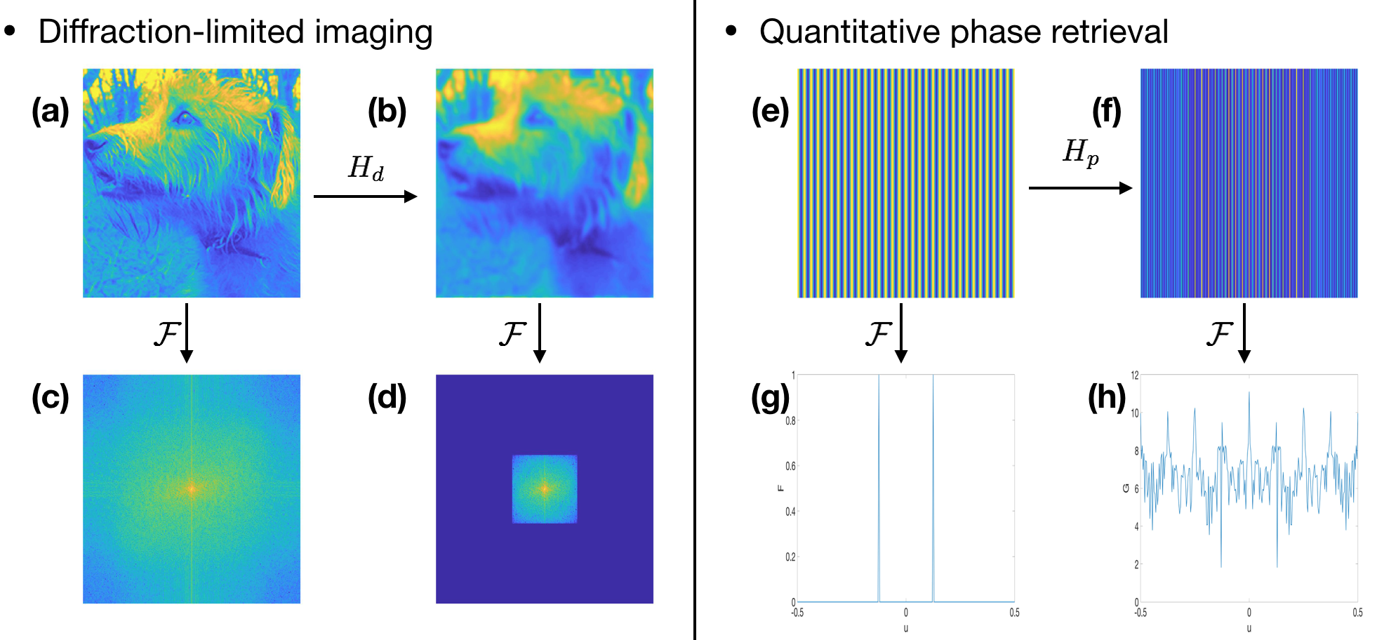
Here, and are the Fourier transforms of and , respectively; and denote the 2D spatial frequencies; and denotes the two dimensional triangular function. As shown in Fig.1, high frequency information beyond cutoff is lost, making the forward operator ill-posed. Here we considered DLI only; generally, the situation becomes worse due to aberrations and other imperfections in the optical system.
Because of the nonlinearity in QPR, it may be thought of as a self-convolution in the frequency domain. To demonstrate this, we show one example in Fig.1. We assume the phase object to be a sinusoidal grating, which contains only a single frequency. However, more than one frequency components exist in the measurement, as can be observed in Fig.1 (h). This frequency scrambling, together with the loss of spatial frequencies due to the finite numerical aperture make the forward operator ill-posed.
4 Proposed Method
4.1 Learning Synthesis by Deep Neural Networks (LS-DNN)
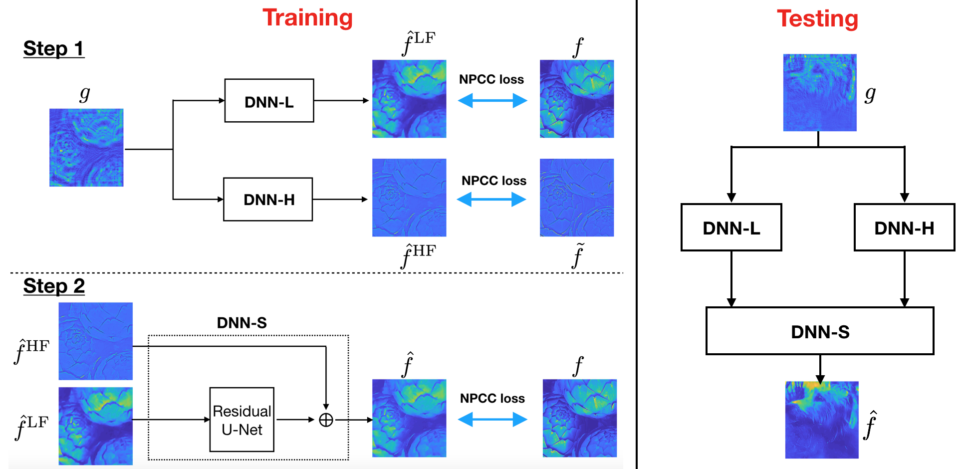
We propose a two-step approach (Fig.2) to tackle the difficulty in restoring high frequency components. First, we use two separate deep neural networks (DNNs) parallel,DNN-L and DNN-H. DNN-L is what typically exists in previous works – it learns to map from the measurements to the un-filtered ground truth images; while DNN-H takes in measurements and maps them to a frequency-modulated ground truth. The modulation in the frequency domain (see Section 4.2), amplifies the relative weights of the high spatial frequencies, thereby facilitating the extraction of high frequencies from the priors.
We expect the reconstruction by DNN-L to be reliable in the low frequency range but not in the high frequency range; whereas the one by DNN-H should be better in the high-frequency range but distorting the low frequency range and may be creating hallucination artifacts. The training of DNN-L and DNN-H can be done in parallel. We denote the reconstructions by DNN-L and DNN-H, during training, as and , respectively.
Moreover, we train a third DNN, denoted as DNN-S, which learns to synthesize the low frequency and high frequency reconstructions from the previous networks and , to generate the final reconstruction matching the un-modulated ground truth.
4.2 Spectral Pre-modulation
The 2D PSD of ImageNet database is well represented as . Therefore, we pre-modulate the ImageNet images with spatial filter , The modulated ground truth has Fourier transform , where denotes the Fourier transform of an un-modulated ground truth image and controls whether high or low frequencies should be enhanced. The optimal value of is determined empirically and we find that DNN-S is robust enough to the choice of without perceptible difference in the reconstructions. In the results shown below in Section 5, we use for SR in DLI and for QPR. Examples of an image in ImageNet and its pre-modulated versions with and are shown in Fig.3.

4.3 Architectures of Deep Neural Networks
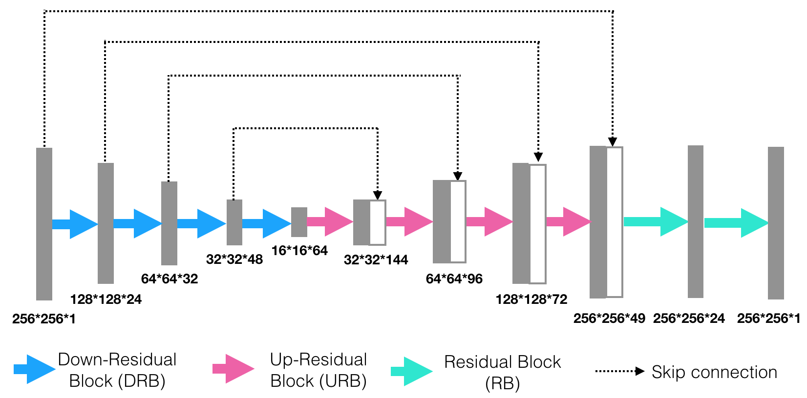
DNN-L and DNN-H follow the same U-Net architecture [33] and utilize residuals to facilitate information flow [20]. As shown in Fig.4, the input to both neural networks is the measurement with size 256x256x1, which is subsequently passed through four successive down-residual blocks (DRBs) for feature extraction. The extracted features pass through 4 up-residual blocks (URBs) and two residual blocks (RBs) for pixel-wise regression to size 256x256x1. Details of architectures of DRBs, URBs, and RBs can be found in the Supplement (Fig.A1). DNN-L is trained with the un-modulated ground truth while DNN-H is trained with the frequency pre-modulated version of the ground truth , as described in Section 4.2.
DNN-S takes in and as inputs. To best preserve the high frequency information contained in , we do not have it pass through most layers of DNN-S. Instead, it only adds to the final outcome of passing through the Residual U-Net (Fig.4) to form the final reconstruction . In other words, the DNN-S trains to map to a variant of itself that removes artifacts brought up by and (conceptually) synthesizes the low-frequency components contained in and the high-frequency components contained in . A potential variation of DNN-S is to make it structurally the same as DNN-L (and DNN-H), except for the input to be instead the concatenation of and (256x256x2) so that they both pass through all successive layers in the DNN. However, due to the low-frequency dominant nature of the DNN-S ground truth examples, exposure of to trainable convolutional filters may cause loss of high frequency information contained in , as in DNN-L. This is why we opted for the first variant.
5 Results

5.1 Implementation details
Training and Test Data
10,000 ImageNet[35] images are used for training (9,000 for training and 1,000 for validation) and 100 ImageNet images and separately designed images for resolution test are used for testing. Measurement is obtained either synthetically (SR in DLI) or experimentally (QPR). For SR in DLI, the nominal resolving ability is set to be pixels. To apply the blur kernel properly, the ground truth is upsampled to before the blur kernel is applied and the outcome is then downsampled to to be the measurement used in DNN-L and DNN-H. In the case of QPR, and . In each training pair, the ground truth is a phase calibrated ImageNet image and the corresponding measurement is obtained by first subtracting a background pattern (also obtained experimentally) and then normalization, before being fed into the LS-DNN architecture.
Negative Pearson Correlation Coefficient (NPCC) as the loss function
We use the Negative Pearson Correlation Coefficient (NPCC) as the loss function to train all the neural networks mentioned above. If denotes the index in the training batch, and denotes the pixel in a particular image, then the batch-wise NPCC loss is defined as:
| (6) | ||||
Here, denotes spatial averaging. Since NPCC only converges to the reconstruction within an affine transform, an additional histogram matching step [25] is performed.
Optimization
The simulation is conducted on a Nvidia GTX1080 GPU using TensorFlow[1]. Adam optimizer[22] is used in the optimization of each deep neural network. Each neural network is trained for 20 epochs and the batch size is 10.

5.2 Reconstruction Results – Spatial Domain
Figs.5 and 6 show test results for DLI and QPR, respectively. DNN-L, DNN-H and DNN-S label the outputs of the corresponding DNNs. In both scenarios, DNN-H succeeds in preserving high frequency components better than DNN-L, as expected, and the DNN-S removes the artifacts introduced by DNN-H through combining with the the low-frequency components captured well by DNN-L. More results are available in Supplement (Figs.A2,A3). Quantitative comparisons for the DNN-L and DNN-S outputs on the entire test images are shown in Table.1. DNN-L actually has better quantitative performance in the problem of SR in DLI. This results verifies the well-known fact that neither PSNR nor SSIM is a good performance metric for visual quality[19, 41, 42, 21, 24].
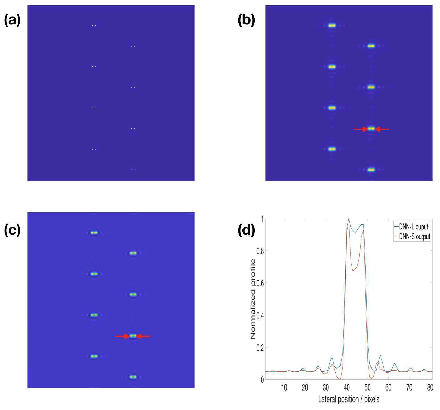
Dot patterns are also used to test the resolution achieved by LS-DNN. The resolution test result for DLI is shown in Fig.7. In the test pattern, the spacing between two nearby dots is pixels, which is beyond the resolving ability of the DLI system ( pixels). While the DNN-L reconstruction failed to distinguish the nearby dots, DNN-S output successfully resolves them. Even though the reconstructions in DNN-L already achieve super-resolution (Supplement Fig.A4), this result demonstrates that DNN-S improves the SR factor even further. The resolution test for phase retrieval is available in the Supplement (Fig.A5), and supports the same conclusion.
To demonstrate that performance improvement of DNN-S over DNN-L is a not a sole consequence of computational capacity increase, we design another ResNet, DNN-L-3, which has the same architecture but twice as many feature maps (except in the last residual block) on each convolutional layer as its counterpart in DNN-L. The resulting DNN-L-3 has more than three times as many trainable parameters as DNN-L(or DNN-H, DNN-S). Reconstructions by DNN-L-3 are compared to those by DNN-S (Supplement Figs.A6, A7.) The superiority of DNN-S results proves our claim.
|
|
|||||
|---|---|---|---|---|---|---|
|
22.9622/0.5545 | 19.9480/0.5210 | ||||
|
18.7531/0.3684 | 18.8525/0.3884 |
5.3 Reconstruction Results – Frequency Domain
Next we analyze LS-DNN performance in the frequency domain. Figs.A8, A9 in the Supplement show the 2D Fourier spectra of the images in Figs.5 and 6, respectively. We find in both DLI and QPR scenarios that, as expected, while DNN-L works well in the low frequency range but fails to recover the high frequency components, DNN-H is better at retrieving the high frequency components but loses some low frequency information. DNN-S serves as a learned synthesizer of the DNN-L and DNN-H outputs at all frequency bands, low and high.
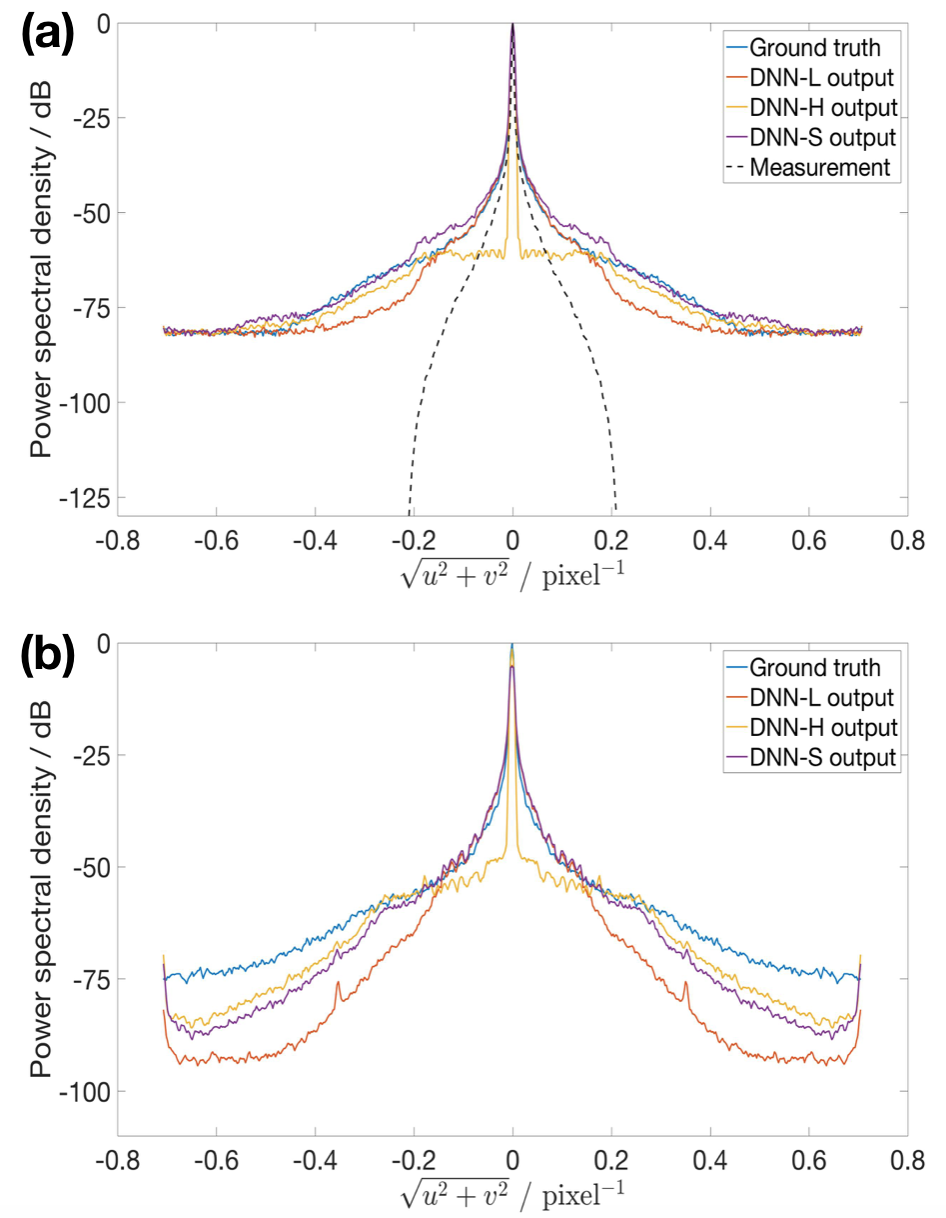
To investigate the performance of our approach on the entire test dataset, we compute the 2D power spectral density (PSD) for the reconstructions of the entire ensemble of the test images and show the 1D cross-sections (along the diagonal direction) in Fig.8. As expected, in both cases, the PSD for the DNN-L output matches well with the ground truth in the low frequency range but is much lower than the ground truth in the high frequency range. Notably, in the case of DLI, the point that the performance of DNN-L starts to drop almost coincides with the cutoff frequency in the measurement. The PSD for DNN-H output is getting closer to the ground truth in the high frequency range than the DNN-L output, benefiting from training data pre-modulation. However, it is much worse in the low frequency range. The DNN-S output, which takes the advantage of both DNN-L and DNN-H, has a PSD that is close to the ground truth within the entire frequency range.
5.4 Comparison with Perceptual Loss Strategy
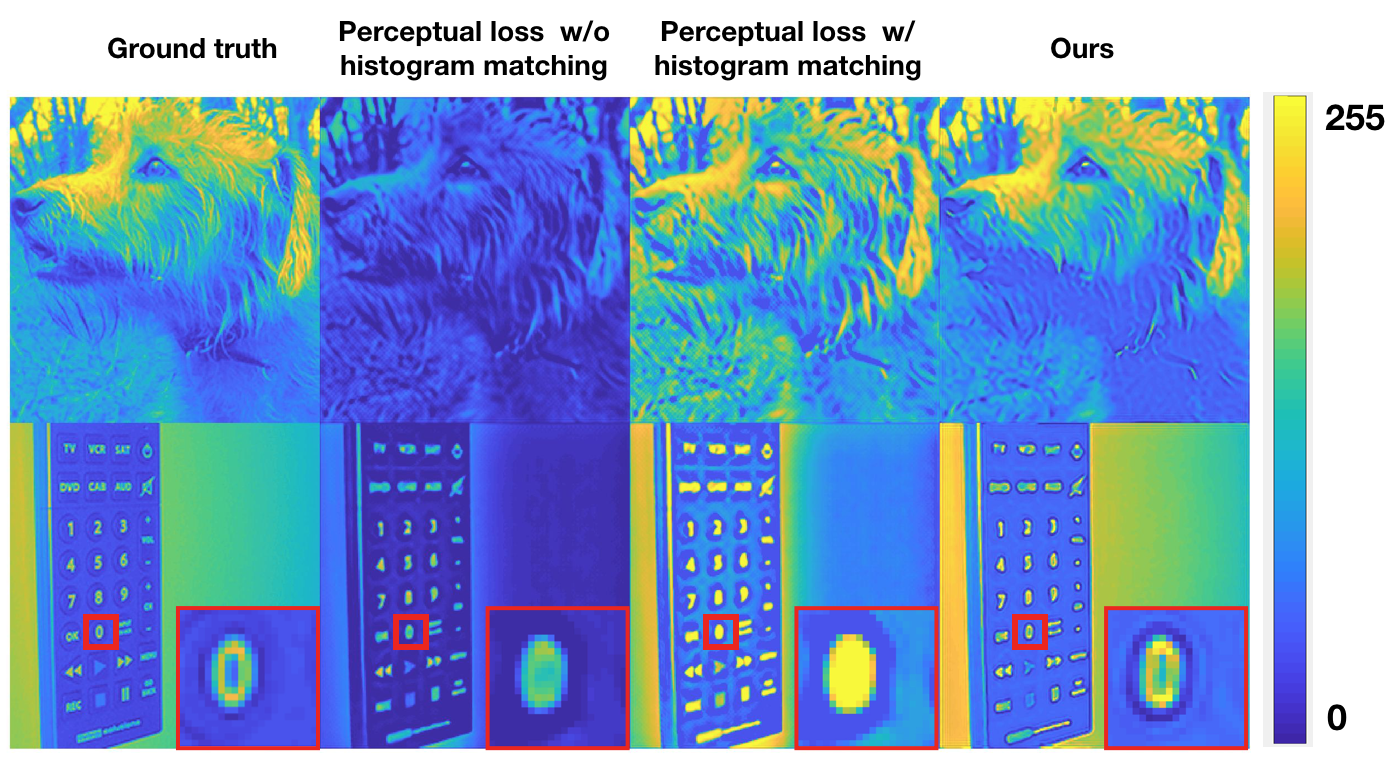
Methods with VGG [37]-based perceptual loss [21, 24], rather than pixel-wise (low-level), as the training loss function, have emerged as most promising approaches for fine detail enhancement in image reconstruction. We conduct a comparison of our DNN-S results with those obtained in [21], in the problem of SR in DLI. The DNN that we use for the perceptual loss strategy is DNN-L-3, so that the perceptual loss approach is not at a disadvantage in terms of computational capacity. Due to the unclear description of the histogram matching step in [21], we present the results by perceptual loss strategy before and after a histogram matching step according to the widely used polynomial-fit scheme (Supplement Section S7 and Fig.A10). From Fig.9, our results are visually better than those by [21], with and without histogram matching. More comparison results available in Supplement Fig.A11. We also compare our results with those by using DNN-L for perceptual loss (Supplement Fig.A12). Our reconstructions perform better in the reconstruction of fine details, without adding undesired high-frequency artifacts.
5.5 Comparison with DualCNN
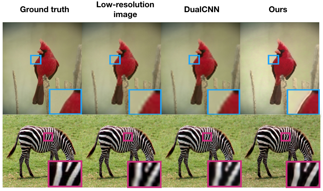
Lastly, we compare our approach with DualCNN [30] for SR interpreted as upsampling, as used in [30]. To ensure a fair comparison, we used the same dataset (BSDS500), upsampling ratio (), pre-processing of data and neural network architectures for DNN-L and DNN-H as in [30].
The comparison results are shown in Fig.10 and Table.2 (and more in Supplement Fig.A13), where visually better results are generated by our approach in Fig.10, though Table.2 demonstrates DualCNN achieves a better quantitative performance, which is not the main objective of this work. This again verifies the well-known fact that neither PSNR nor SSIM is a good performance metric for visual quality[19, 41, 42, 21, 24].
| Dual CNN | Ours | |
|---|---|---|
| PSNR/SSIM | 24.5657/0.7953 | 22.4155/0.7771 |
6 Conclusions
We have proposed a novel LS-DNN architecture that leverages the learning capability of a neural network to optimally synthesize parallel reconstructions that are reliable on low and high frequencies, respectively. The results verified our idea and showed reconstructions of better visual quality than the perceptual loss [21] approach, as well as the more conceptually similar to ours DualCNN approach[30].
The LS-DNN methodology is applicable to many other ill-posed image recovery problems, when there is imbalance between the spatial frequency region where the forward operator suppresses or loses content and the availability of content in the same frequency range in the training database to compensate. Generalizations may also be possible, for example to more than two frequency bands, similarly trained separately with pre-filtering and recombined in learned fashion; however, splitting the frequency bands too finely may be counterproductive if it results in too many parameters to learn. This is an interesting topic for future work.
References
- [1] M. Abadi, A. Agarwal, P. Barham, E. Brevdo, Z. Chen, C. Citro, G. S. Corrado, A. Davis, J. Dean, M. Devin, S. Ghemawat, I. Goodfellow, A. Harp, G. Irving, M. Isard, Y. Jia, R. Jozefowicz, L. Kaiser, M. Kudlur, J. Levenberg, D. Mané, R. Monga, S. Moore, D. Murray, C. Olah, M. Schuster, J. Shlens, B. Steiner, I. Sutskever, K. Talwar, P. Tucker, V. Vanhoucke, V. Vasudevan, F. Viégas, O. Vinyals, P. Warden, M. Wattenberg, M. Wicke, Y. Yu, and X. Zheng. TensorFlow: Large-scale machine learning on heterogeneous systems, 2015. Software available from tensorflow.org.
- [2] M. Aharon, M. Elad, and A. Bruckstein. K-svd: An algorithm for designing overcomplete dictionaries for sparse representation. IEEE Transactions on signal processing, 54(11):4311, 2006.
- [3] J. Bruna, P. Sprechmann, and Y. LeCun. Super-resolution with deep convolutional sufficient statistics. arXiv preprint arXiv:1511.05666, 2015.
- [4] E. Candès, J. Romberg, and T. Tao. Robust uncertainty principles: Exact signal reconstruction from highly incomplete fourier information. IEEE Trans. Inform. Theory, 52(2):489–509, 2006.
- [5] E. Candès, J. Romberg, and T. Tao. Stable signal recovery from incomplete and inaccurate measurements. Comm. Pure Appl. Math., 59(8):1207–1223, 2006.
- [6] E. Candès and T. Tao. Near optimal signal recovery from random projections: Universal encoding strategies? IEEE Trans. Inform. Theory, 52(12):5406–5425, 2006.
- [7] K. Creath. Phase-shifting speckle interferometry. Applied Optics, 24(18):3053–3058, 1985.
- [8] C. Dong, C. C. Loy, K. He, and X. Tang. Learning a deep convolutional network for image super-resolution. In European conference on computer vision, pages 184–199. Springer, 2014.
- [9] D. L. Donoho. Compressed sensing. IEEE Transactions on information theory, 52(4):1289–1306, 2006.
- [10] A. Dosovitskiy and T. Brox. Generating images with perceptual similarity metrics based on deep networks. In Advances in Neural Information Processing Systems, pages 658–666, 2016.
- [11] M. Elad and M. Aharon. Image denoising via learned dictionaries and sparse representation. In 2006 IEEE Computer Society Conference on Computer Vision and Pattern Recognition, volume 1, pages 895–900. IEEE, 2006.
- [12] L. Gatys, A. S. Ecker, and M. Bethge. Texture synthesis using convolutional neural networks. In Advances in Neural Information Processing Systems, pages 262–270, 2015.
- [13] R. W. Gerchberg. A practical algorithm for the determination of phase from image and diffraction plane pictures. Optik, 35:237–246, 1972.
- [14] I. Goodfellow, J. Pouget-Abadie, M. Mirza, B. Xu, D. Warde-Farley, S. Ozair, A. Courville, and Y. Bengio. Generative adversarial nets. In Advances in neural information processing systems, pages 2672–2680, 2014.
- [15] J. W. Goodman. Introduction to Fourier optics. Roberts and Company Publishers, 2005.
- [16] J. W. Goodman and R. Lawrence. Digital image formation from electronically detected holograms. Applied physics letters, 11(3):77–79, 1967.
- [17] A. Goy, K. Arthur, S. Li, and G. Barbastathis. Low photon count phase retrieval using deep learning. arXiv preprint arXiv:1806.10029, 2018.
- [18] K. Gregor and Y. LeCun. Learning fast approximations of sparse coding. In Proceedings of the 27th International Conference on International Conference on Machine Learning, pages 399–406. Omnipress, 2010.
- [19] P. Gupta, P. Srivastava, S. Bhardwaj, and V. Bhateja. A modified psnr metric based on hvs for quality assessment of color images. In Communication and Industrial Application (ICCIA), 2011 International Conference on, pages 1–4. IEEE, 2011.
- [20] K. He, X. Zhang, S. Ren, and J. Sun. Deep residual learning for image recognition. In Proceedings of the IEEE conference on computer vision and pattern recognition, pages 770–778, 2016.
- [21] J. Johnson, A. Alahi, and L. Fei-Fei. Perceptual losses for real-time style transfer and super-resolution. In European Conference on Computer Vision, pages 694–711. Springer, 2016.
- [22] D. P. Kingma and J. Ba. Adam: A method for stochastic optimization. arXiv preprint arXiv:1412.6980, 2014.
- [23] Y. LeCun, Y. Bengio, and G. Hinton. Deep learning. nature, 521(7553):436, 2015.
- [24] C. Ledig, L. Theis, F. Huszár, J. Caballero, A. Cunningham, A. Acosta, A. P. Aitken, A. Tejani, J. Totz, Z. Wang, et al. Photo-realistic single image super-resolution using a generative adversarial network. In CVPR, volume 2, page 4, 2017.
- [25] S. Li and G. Barbastathis. Spectral pre-modulation of training examples enhances the spatial resolution of the phase extraction neural network (phenn). Optics Express, 26(22):29340–29352, 2018.
- [26] D. Lim, K. K. Chu, and J. Mertz. Wide-field fluorescence sectioning with hybrid speckle and uniform-illumination microscopy. Optics letters, 33(16):1819–1821, 2008.
- [27] A. Mahendran and A. Vedaldi. Understanding deep image representations by inverting them. In Proceedings of the IEEE conference on computer vision and pattern recognition, pages 5188–5196, 2015.
- [28] M. Mardani, H. Monajemi, V. Papyan, S. Vasanawala, D. Donoho, and J. Pauly. Recurrent generative residual networks for proximal learning and automated compressive image recovery. arXiv:1711.10046, 11 2017.
- [29] M. Mathieu, C. Couprie, and Y. LeCun. Deep multi-scale video prediction beyond mean square error. arXiv preprint arXiv:1511.05440, 2015.
- [30] J. Pan, S. Liu, D. Sun, J. Zhang, Y. Liu, J. Ren, Z. Li, J. Tang, H. Lu, Y.-W. Tai, and M.-H. Yang. Learning dual convolutional neural networks for low-level vision. In The IEEE Conference on Computer Vision and Pattern Recognition (CVPR), June 2018.
- [31] Y. Rivenson, Z. Göröcs, H. Günaydin, Y. Zhang, H. Wang, and A. Ozcan. Deep learning microscopy. Optica, 4(11):1437–1443, 2017.
- [32] Y. Rivenson, Y. Zhang, H. Günaydın, D. Teng, and A. Ozcan. Phase recovery and holographic image reconstruction using deep learning in neural networks. Light: Science & Applications, 7(2):17141, 2018.
- [33] O. Ronneberger, P. Fischer, and T. Brox. U-net: Convolutional networks for biomedical image segmentation. In International Conference on Medical image computing and computer-assisted intervention, pages 234–241. Springer, 2015.
- [34] R. Rubinstein, A. M. Bruckstein, and M. Elad. Dictionaries for sparse representation modeling. Proceedings of the IEEE, 98(6):1045–1057, 2010.
- [35] O. Russakovsky, J. Deng, H. Su, J. Krause, S. Satheesh, S. Ma, Z. Huang, A. Karpathy, A. Khosla, M. Bernstein, et al. Imagenet large scale visual recognition challenge. International Journal of Computer Vision, 115(3):211–252, 2015.
- [36] K. Simonyan, A. Vedaldi, and A. Zisserman. Deep inside convolutional networks: Visualising image classification models and saliency maps. arXiv preprint arXiv:1312.6034, 2013.
- [37] K. Simonyan and A. Zisserman. Very deep convolutional networks for large-scale image recognition. arXiv preprint arXiv:1409.1556, 2014.
- [38] A. Sinha, J. Lee, S. Li, and G. Barbastathis. Lensless computational imaging through deep learning. Optica, 4(9):1117–1125, 2017.
- [39] M. R. Teague. Deterministic phase retrieval: a green’s function solution. JOSA, 73(11):1434–1441, 1983.
- [40] A. van der Schaaf and J. H. van Hateren. Modelling the power spectra of natural images: statistics and information. Vision research, 36(17):2759–2770, 1996.
- [41] Z. Wang, A. C. Bovik, H. R. Sheikh, and E. P. Simoncelli. Image quality assessment: from error visibility to structural similarity. IEEE transactions on image processing, 13(4):600–612, 2004.
- [42] Z. Wang, E. P. Simoncelli, and A. C. Bovik. Multiscale structural similarity for image quality assessment. In The Thrity-Seventh Asilomar Conference on Signals, Systems & Computers, 2003, volume 2, pages 1398–1402. Ieee, 2003.
- [43] C.-Y. Yang, C. Ma, and M.-H. Yang. Single-image super-resolution: A benchmark. In European Conference on Computer Vision, pages 372–386. Springer, 2014.
- [44] J. Yosinski, J. Clune, A. Nguyen, T. Fuchs, and H. Lipson. Understanding neural networks through deep visualization. arXiv preprint arXiv:1506.06579, 2015.