Non-perturbative probability distribution function for cosmological counts in cells

Abstract

We present a non-perturbative calculation of the 1-point probability distribution function (PDF) for the spherically-averaged matter density field. The PDF is represented as a path integral and is evaluated using the saddle-point method. It factorizes into an exponent given by a spherically symmetric saddle-point solution and a prefactor produced by fluctuations. The exponent encodes the leading sensitivity of the PDF to the dynamics of gravitational clustering and statistics of the initial conditions. In contrast, the prefactor has only a weak dependence on cosmology. It splits into a monopole contribution which is evaluated exactly, and a factor corresponding to aspherical fluctuations. The latter is crucial for the consistency of the calculation: neglecting it would make the PDF incompatible with translational invariance. We compute the aspherical prefactor using a combination of analytic and numerical techniques. We demonstrate the factorization of spurious enhanced contributions of large bulk flows and their cancellation due to the equivalence principle. We also identify the sensitivity to the short-scale physics and argue that it must be properly renormalized. The uncertainty associated with the renormalization procedure gives an estimate of the theoretical error. For zero redshift, the precision varies from sub percent for moderate density contrasts to tens of percent at the tails of the distribution. It improves at higher redshifts. We compare our results with N-body simulation data and find an excellent agreement.

1 Introduction

Current and planned cosmological surveys are going to map the large-scale structure (LSS) of the universe with unprecedented precision at a wide range of scales and redshifts. These data will potentially carry a wealth of information on cosmological parameters, the initial conditions of the universe, the properties of dark matter and dark energy. Extracting this information requires accurate quantitative understanding of matter clustering in the non-linear regime, both in the standard $\Lambda$CDM cosmology, as well as its extensions.

The direct approach relies on numerical N-body simulations that have made an impressive progress in the last decades. However, reaching the required level of accuracy still remains computationally expensive [1]. Moreover, while the N-body methods have been well adapted to the $\Lambda$CDM cosmology, their modification to include the effects of new physics is often extremely demanding. This calls for development of the analytic approaches to LSS. Being perhaps less powerful than N-body simulations in the description of the $\Lambda$CDM cosmology, the analytic approach provides more flexibility in going beyond it and a deeper insight in the relevance of different physical processes. Hence, analytic and N-body methods are complementary to each other.

The most developed analytic approach to LSS is the cosmological perturbation theory, where the evolution equations for the density and velocity fields are solved iteratively treating the density contrast as a small quantity. The correlation functions of cosmological observables are then evaluated by averaging over the initial conditions [2]. An intensive research in this direction in recent years has clarified various physical effects. The developments include understanding the role of the equivalence principle in the cancellation of the so-called ‘IR-divergences’ [3, 4, 5, 6, 7, 8, 9], accurate treatment of the effects of large bulk flows on baryon acoustic oscillations [10, 11, 12, 13] and systematic accounting for the contribution of non-linear density inhomogeneities at short scales along the lines of effective field theory (EFT) [14, 15, 16, 17, 18, 19]. As a result of this progress a sub-percent-level precision has been achieved in perturbative calculation of the matter power spectrum and bispectrum for comoving wavenumbers $k\lesssim 0.1h/\rm{Mpc}$.

In this paper we show that the analytic approach can be rigorously extended beyond perturbation theory. The non-perturbative observable that we are going to consider is counts-in-cells statistics (see e.g. [20]).

The counts-in-cells method amounts to splitting the cosmic density field into cells in position space and taking an aggregate of this field inside each cell. In the case of discrete tracers one counts the number of objects inside each cell. The distribution of cells over the relevant variable reveals statistical properties of the underlying field. In this paper we discuss the 1-point probability distribution function (PDF) of finding a certain average matter density in a sphere of a given fixed radius $r_{*}$. The deviation of this spherically-averaged density from the mean density of the universe does not need to be small, and thus the desired PDF cannot be calculated within perturbation theory.

Formally, the count-in-cells statistics include information from all n-point functions of the density field in a compressed way which facilitates measurements, but looses the information encoded in the shape dependence of the n-point correlators. Therefore, it is complementary to perturbative methods in the information content.

The counts-in-cells statistics are one of the classic observables in LSS. The distribution of galaxies in 2-dimensional angular cells on the sky was first measured by E. Hubble [21], who noticed that it is close to log-normal. For the total matter density this has been recently tested in [22, 23]. The log-normal distribution was also suggested as a model for the 1-point PDF in the case of three-dimensional cells [24] and has been quite successful in describing both N-body simulations [25, 26] and observational data [27, 28]. However, as pointed out in [29, 30], this success appears to be accidental and is due to the specific shape of the power spectrum at mildly non-linear scales. Recent high-accuracy N-body simulations performed in [31] revealed significant deviations of the measured PDF from the log-normal fit.

Pioneering calculations of the counts-in-cells PDF from first principles were performed in Refs. [32, 29] using insights from perturbation theory. This study was extended beyond perturbation theory in Refs. [33, 34, 35, 36], where it was argued that the most probable dynamics producing a given overdensity in a spherical cell respects the symmetry of the problem, i.e. it is given by a spherical collapse. Recently, these calculations were revisited in the context of the Large Deviation Principle (LDP) [37]. In particular, Ref. [38] introduced the logarithmic density transformation to avoid certain problems associated with the application of LDP directly to the density PDF [39]. This formalism has been applied to joint PDF of densities in two cells [40, 41, 42] and to biased tracers [43]. An alternative approach to the counts-in-cells statistics developed in [44, 45, 46] is based on the Lagrangian-space description of LSS. Ref. [47] recently derived 1-point PDF in a toy model of $(1+1)$ dimensional universe. Counts-in-cells statistics were suggested as promising probes of primordial non-Gaussianity [48, 49] and as a suitable tool to analyze the future 21 cm intensity mapping data [50].

In this paper we pursue the path-integral approach to counts-in-cells pioneered in [48, 35, 36]. In this approach the calculation of the 1-point PDF closely resembles a calculation of instanton effects in quantum field theory (QFT). Following Ref. [9] we introduce a formal parameter characterizing the overall amplitude of the matter power spectrum and argue that it plays a role of the coupling constant in the theory. When the coupling is small, the path integral defining the 1-point PDF can be evaluated in the saddle-point (‘semiclassical’) approximation. Thereby the PDF factorizes into the exponential part given by the leading saddle-point configuration and a prefactor coming from integration over small fluctuations around the saddle-point solution. We confirm the assertion [35, 36] that the saddle-point configuration corresponds to the spherically symmetric dynamics. In this way we recover the well-known result [35, 45, 46, 37, 38] for the leading exponential part of the PDF. Our key result is computation of the prefactor due to aspherical perturbations around the spherical collapse which has not been done in the previous works. We demonstrate that this ‘aspherical prefactor’ is crucial for the consistency of the saddle-point calculation. In particular, it is required to ensure that the mean value of the density contrast vanishes.

In the QFT analogy, evaluation of the aspherical prefactor amounts to a 1-loop computation in a non-trivial background. As such, it is instructive in several respects. First, it shows how the vanishing of the mean density contrast is related to the translational invariance of the theory, spontaneously broken by the position of the cell. Second, the sector of dipole perturbations exhibits ‘IR divergences’ at intermediate steps of the calculation associated to large bulk flows. We show that the equivalence principle ensures cancellation of these divergences. We devise a procedure to isolate the IR-enhanced contributions and cancel them analytically, prior to any numerical evaluation. Finally, the contributions of high multipoles are sensitive to short-distance dynamics and must be renormalized. Unfortunately, it is impossible to unambiguously fix the renormalization procedure from first principles. We isolate the ‘UV-divergent’ part of the prefactor and consider two models for its renormalization, differing by the dependence of the corresponding counterterm on the density contrast. Both models use as input the value of the counterterm for the 1-loop power spectrum, and thus do not introduce any new fitting parameters. We suggest to use the difference between the two models as an estimate of the theoretical uncertainty introduced by renormalization. This uncertainty is less than percent in the range of moderate cell densities, $\rho_{\rm cell}/\rho_{\rm univ}\in[0.5,2]$, where $\rho_{\rm univ}$ is the average density of the universe, and degrades to 30% for extreme values $\rho_{\rm cell}/\rho_{\rm univ}=0.1$ or $\rho_{\rm cell}/\rho_{\rm univ}=10$ at $z=0$.

To verify our approach we ran a suite of N-body simulations using the FastPM code [51]. The numerical studies are performed for the following cosmology: a flat $\Lambda$CDM with $\Omega_{m}=0.26$, $\Omega_{b}=0.044$, $h=0.72$, $n_{s}=0.96$, Gaussian initial conditions, $\sigma_{8}=0.794$. This is the same choice as in Ref. [42] which used the counts-in-cells distribution extracted from the Horizon run 4 simulation [52]; it facilitates a direct comparison between our results and those of [42]. Throughout the paper the linear power spectrum is computed with the Boltzmann code CLASS [53].

The predictions of our method are found to be in complete agreement with the results of N-body simulations. First, the 1-point PDF clearly exhibits the semiclassical scaling. The aspherical prefactor extracted from the N-body data shows a very weak dependence on redshift or the radius of the cell, as predicted by theory. Second, the data fall inside the range spanned by our theoretical uncertainty. Remarkably, one of the counterterm models matches the data within the accuracy of the simulations throughout the whole range of available densities, $\rho_{\rm cell}/\rho_{\rm univ}\in[0.1,10]$, at all redshifts and for different cell radii.

The paper is organized as follows. In Sec. 2 we introduce the path integral representation of the 1-point PDF, identify its saddle point and demonstrate the factorization of the PDF into the leading exponent and prefactor. We evaluate the leading exponential part. In Sec. 3 we evaluate explicitly the prefactor due to spherically symmetric perturbations and discuss the general properties of the aspherical prefactor. We compare the theoretical expectations with the prefactor extracted from the N-body data and provide simple fitting formulas for it. The rest of the paper is devoted to the calculation of the aspherical prefactor from first principles. In Sec. 4 we compute the aspherical prefactor at small values of the density contrast using perturbation theory. In Sec. 5 we derive the set of equations describing the prefactor in the non-perturbative regime of large density contrasts and present an algorithm for its numerical evaluation. In Sec. 6 we modify the algorithm for the sector of dipole perturbations in order to explicitly factor out and cancel the IR-enhanced contributions. In Sec. 7 we compute the contributions of high multipoles using the Wentzel–Kramers–Brillouin (WKB) approximation. In Sec. 8 we present our numerical results for the aspherical prefactor, discuss the contribution of short-distance physics and its renormalization. Section 9 contains a summary of our results and discussion.

Several appendices contain supplementary material. Appendix A summarizes our conventions. Appendix B is devoted to the details of our N-body simulations. In Appendix C we review the dynamics of spherical collapse in Einstein–de Sitter (EdS) and $\Lambda$CDM universes. In Appendix D we derive a useful formula for the determinant of matrices of a special form. Appendix E contains equations for the aspherical prefactor in $\Lambda$CDM cosmology. Some technical aspects of the WKB calculation of the high-multipole contributions are discussed in Appendix F. Appendix G contains details of our numerical procedure. In Appendix H we comment on the log-normal model for the counts-in-cells statistics.

2 Path integral for counts-in-cells PDF

2.1 Spherical collapse saddle point

Consider the density contrast averaged over a spherical cell of radius $r_{*}$,

$$\bar{\delta}_{W}=\int\frac{d^{3}x}{r_{*}^{3}}\,\tilde{W}(r/r_{*})\,\delta({\bf x})=\int_{\bf k}W(kr_{*})\delta({\bf k})\,,$$ (2.1)

where $\delta({\bf x})\equiv\frac{\delta\rho({\bf x})}{\rho_{\rm univ}}$, $\tilde{W}(r/r_{*})$ is a window function, $W(kr_{*})$ is its Fourier transform, and we have introduced the notation $\int_{\bf k}\equiv\int\frac{d^{3}k}{(2\pi)^{3}}$. We will soon specify the window function to be top-hat in the position space, which is the standard choice for counts-in-cells statistics. However, it is instructive to see how far one can proceed without making any specific assumptions about $\tilde{W}$, apart from it being spherically symmetric. The window function is normalized as

$$\int\frac{d^{3}x}{r_{*}^{3}}\,\tilde{W}(r/r_{*})=1\,.$$ (2.2)

We are interested in the 1-point PDF $\mathcal{P}(\delta_{*})$ describing the probability that the random variable $\bar{\delta}_{W}$ takes a given value $\delta_{*}$. Due to translational invariance, the 1-point statistics do not depend on the position of the cell. Thus, without loss of generality we center the cell at the origin, ${\bf x}=0$.

We assume that the initial conditions for the density perturbations at some large redshift $z_{i}$ are adiabatic and Gaussian, so that their statistical properties are fully determined by the 2-point cumulant,

$$\langle\delta_{i}({\bf k})\delta_{i}({\bf k}^{\prime})\rangle=(2\pi)^{3}\delta^{(3)}_{\rm D}({\bf k}+{\bf k}^{\prime})\,g^{2}(z_{i})\,P(k)\,,$$ (2.3)

where $\delta_{\rm D}^{(3)}$ is the 3-dimensional Dirac delta-function. Here $P(k)$ is the linear power spectrum at redshift zero and $g(z)$ is the linear growth factor. The latter is normalized to be 1 at $z=0$. Nevertheless, it is convenient to keep $g^{2}$ explicitly in the formulas and treat it as a small free parameter. The rationale behind this approach is to use $g^{2}$ as a book-keeping parameter that characterizes the overall amplitude of the power spectrum and thereby controls the saddle-point evaluation of the PDF, just like a coupling constant controls the semiclassical expansion in QFT (cf. [9]). The true physical expansion parameter in our case is the smoothed density variance at the scale $r_{*}$, as will become clear shortly.

Instead of working directly with the initial density field $\delta_{i}$, it is customary to rescale it to redshift $z$ using the linear growth factor,

$$\delta_{L}({\bf k},z)=\frac{g(z)}{g(z_{i})}\delta_{i}({\bf k})\,.$$ (2.4)

We will refer to $\delta_{L}$ as the ‘linear density field’ in what follows and will omit the explicit $z$-dependence to simplify notations.

The desired PDF is given by the following path integral [35, 48],

$$\mathcal{P}(\delta_{*})={\cal N}^{-1}\int\mathscr{D}\delta_{L}\exp\left\{-\int_{\bf k}\frac{|\delta_{L}({\bf k})|^{2}}{2g^{2}P(k)}\right\}\,\delta^{(1)}_{\rm D}\big{(}\delta_{*}-\bar{\delta}_{W}[\delta_{L}]\big{)}\,,$$ (2.5)

where different linear density perturbations are weighted with the appropriate Gaussian weight. The Dirac delta-function ensures that only the configurations that produce the average density contrast $\delta_{*}$ are retained in the integration. Note that we have written $\bar{\delta}_{W}$ as a functional of the linear density field, $\bar{\delta}_{W}[\delta_{L}]$. In general, this functional is complicated and its evaluation requires knowing non-linear dynamics that map initial linear perturbations onto the final non-linear density field $\delta({\bf x})$. The normalization factor in (2.5) is

$$\mathcal{N}=\int\mathscr{D}\delta_{L}\exp\bigg{\{}-\int_{\bf k}\frac{|\delta_{L}({\bf k})|^{2}}{2g^{2}P(k)}\bigg{\}}\,.$$ (2.6)

It is convenient to rewrite the delta-function constraint using the inverse Laplace transform,

$$\mathcal{P}(\delta_{*})={\cal N}^{-1}\int_{-i\infty}^{i\infty}\frac{d\lambda}{2\pi ig^{2}}\int\mathscr{D}\delta_{L}\exp\bigg{\{}-\frac{1}{g^{2}}\bigg{[}\int_{\bf k}\frac{|\delta_{L}({\bf k})|^{2}}{2P(k)}-\lambda\big{(}\delta_{*}-\bar{\delta}_{W}[\delta_{L}]\big{)}\bigg{]}\bigg{\}}\,.$$ (2.7)

where we introduced the Lagrange multiplier $\lambda$. Our goal is to compute the above integral by the steepest-decent method. We expect the result to take the form,

$$\mathcal{P}(\delta_{*})=\exp\left\{-\frac{1}{g^{2}}\left(\alpha_{0}+\alpha_{1}g^{2}+\alpha_{2}g^{4}+...\right)\right\}\,.$$ (2.8)

The leading term $\alpha_{0}$ corresponds to the exponent of the integrand in (2.7) evaluated on the saddle-point configuration. The first correction $\alpha_{1}g^{2}$ stems from the Gaussian integral around the saddle point. It gives rise to a $g$-independent prefactor in the PDF. As we discuss below, the evaluation of $\alpha_{1}$ corresponds to a one-loop calculation in the saddle-point background. Higher loops give further corrections $\alpha_{2}g^{4}$ etc., which can be rewritten as $O(g^{2})$ corrections to the prefactor. We will not consider them in this paper.

We are looking for a saddle point of the integral (2.7) in the limit $g^{2}\to 0$. Taking variations of the expression in the exponent w.r.t. $\delta_{L}$ and $\lambda$, we obtain the equations for the saddle-point configuration,

$$\frac{\delta_{L}({\bf k})}{P(k)}+\lambda\frac{\partial\bar{\delta}_{W}}{\partial\delta_{L}({\bf k})}=0\,,$$ (2.9a)

$$\bar{\delta}_{W}[\delta_{L}]=\delta_{*}\,.$$ (2.9b)

Now comes a crucial observation: a spherically symmetric Ansatz for $\delta_{L}({\bf k})$ goes through these equations. Let us prove this. The check is non-trivial only for Eq. (2.9a). Clearly, if the linear field is spherically symmetric, the first term in (2.9a) depends only on the absolute value $k$ of the momentum. We need to show that this is also the case for the second term. To this end, expand the variational derivative,

$$\frac{\partial\bar{\delta}_{W}}{\partial\delta_{L}({\bf k})}=\int\frac{d^{3}x}{r_{*}^{3}}\,\tilde{W}(r/r_{*})\,\frac{\partial\delta({\bf x})}{\partial\delta_{L}({\bf k})}\;.$$ (2.10)

Due to rotational invariance of dynamics, the derivative $\partial\delta({\bf x})/\partial\delta_{L}({\bf k})$, evaluated on a spherically symmetric linear density configuration, is a rotationally invariant function of the vectors ${\bf x}$ and ${\bf k}$. Thus, it depends only on the lengths $x$, $k$ and the scalar product $({\bf k}{\bf x})$. Upon integration with a spherically symmetric window function $\tilde{W}$, only the dependence on the absolute value of the momentum $k$ survives. This completes the proof.

The previous observation greatly simplifies the solution of the saddle-point equations (2.9). It implies that we can search for the saddle point among spherically symmetric configurations. For such configurations there exists a simple mapping between the linear and non-linear density fields prior to shell-crossing, see Appendix C. This mapping relates the non-linear density contrast averaged over a cell of radius $r$,

$$\bar{\delta}(r)\equiv\frac{3}{r^{3}}\int_{0}^{r}dr_{1}\,r_{1}^{2}\,\delta(r_{1})\;,$$ (2.11)

with the linear averaged density

$$\bar{\delta}_{L}(R)\equiv\frac{3}{R^{3}}\int_{0}^{R}dR_{1}\,R_{1}^{2}\,\delta_{L}(R_{1})$$ (2.12)

at the radius

$$R=r\big{(}1+\bar{\delta}(r)\big{)}^{1/3}\;.$$ (2.13)

In the last expression one recognizes the Lagrangian radius of the matter shell whose Eulerian radius is $r$. The mapping then gives $\bar{\delta}_{L}(R)$ as a function of $\bar{\delta}(r)$ and vice versa,

$$\bar{\delta}_{L}(R)=F\big{(}\bar{\delta}(r)\big{)}~{}~{}~{}~{}~{}\Longleftrightarrow~{}~{}~{}~{}~{}\bar{\delta}(r)=f\big{(}\bar{\delta}_{L}(R)\big{)}\;.$$ (2.14)

Evaluation of the functions $F$ or $f$ requires an inversion of an elementary analytic function (in EdS cosmology) or solution of a first-order ordinary differential equation (in $\Lambda$CDM). Both operations are easily performed using standard computer packages. Curiously, the mapping (2.14) is almost independent of cosmology (EdS vs. $\Lambda$CDM).

The existence of the mapping (2.14) allows us to compute the variational derivative in Eq. (2.9a) explicitly for spherically symmetric $\delta_{L}(k)$. Assuming that the non-linear density field $\delta(r)$ has not undergone shell-crossing, we transform the expression for $\bar{\delta}_{W}$ as follows,

$$\begin{split}\bar{\delta}_{W}=&\frac{4\pi}{r_{*}^{3}}\int dr\,r^{2}\,\tilde{W}(r/r_{*})\big{(}1+\delta(r)\big{)}-1\\ =&\frac{4\pi}{r_{*}^{3}}\int dR\,R^{2}\tilde{W}\Big{(}R\big{(}1+f\big{(}\bar{\delta}_{L}(R)\big{)}\big{)}^{-1/3}/r_{*}\Big{)}-1\,.\end{split}$$ (2.15)

Taking into account that

$$\bar{\delta}_{L}(R)=\int_{\bf k}\frac{3j_{1}(kR)}{kR}\,\delta_{L}(k)\;,$$ (2.16)

where $j_{1}$ is the spherical Bessel function (see Appendix A for conventions), we obtain,

$$\frac{\partial\bar{\delta}_{W}}{\partial\delta_{L}(k)}=-\frac{4\pi}{r_{*}^{4}k}\int dR\,R^{2}\,\tilde{W}^{\prime}\big{(}R(1+f)^{-1/3}/r_{*}\big{)}\,\frac{f^{\prime}}{(1+f)^{4/3}}\,j_{1}(kR)\;,$$ (2.17)

where primes denote differentiation of the functions w.r.t. their arguments. Here $f$ and $f^{\prime}$ are functions of $\bar{\delta}_{L}(R)$ and hence functionals of $\delta_{L}(k)$. Substituting this expression into (2.9a) we obtain,

$$\delta_{L}(k)=\lambda P(k)\frac{4\pi}{r_{*}^{4}k}\int dR\,R^{2}\frac{\tilde{W}^{\prime}\big{(}R(1+f)^{-1/3}/r_{*}\big{)}\,f^{\prime}\,j_{1}(kR)}{(1+f)^{4/3}}\,.$$ (2.18)

This is a non-linear integral equation for $\delta_{L}(k)$ which can, in principle, be solved numerically. Together with Eq. (2.9b) that fixes the value of the Lagrange multiplier $\lambda$ through the overall normalization of $\delta_{L}(k)$, they form a complete system of equations determining the saddle-point linear density. For a generic window function $\tilde{W}$ the solution of this system appears challenging. We are now going to see that Eq. (2.18) gets drastically simplified for top-hat $\tilde{W}$.

2.2 Leading exponent for top-hat window function

From now on we specify to the case of a top-hat window function in position space,

$$\tilde{W}_{\rm th}(r/r_{*})=\frac{3}{4\pi}\Theta_{\rm H}\left(1-\frac{r}{r_{*}}\right)~{}~{}~{}~{}~{}\Longleftrightarrow~{}~{}~{}~{}~{}W_{\rm th}(kr_{*})=\frac{3j_{1}(kr_{*})}{kr_{*}}\,,$$ (2.19)

where $\Theta_{\text{H}}$ stands for the Heaviside theta-function. As the derivative of $\tilde{W}_{\rm th}$ is proportional to the Dirac delta-function, the integral in (2.18) localizes to $R=R_{*}$, where

$$R_{*}=r_{*}(1+\delta_{*})^{1/3}\;.$$ (2.20)

After a straightforward calculation Eq. (2.18) simplifies to

$$\delta_{L}(k)=-\frac{\lambda}{C}P(k)\,W_{\rm th}(kR_{*})\,$$ (2.21)

with

$$C=F^{\prime}(\delta_{*})+\frac{\bar{\delta}_{L}(R_{*})-\delta_{L}(R_{*})}{1+\delta_{*}}\;.$$ (2.22)

Here $F$ is the spherical-collapse mapping function introduced in (2.14) and in deriving (2.21), (2.22) we have used the relation,

$$F^{\prime}(\delta_{*})=\frac{1}{f^{\prime}\big{(}\bar{\delta}_{L}(R_{*})\big{)}}\;.$$

One observes that (2.21) fixes the $k$-dependence of the saddle-point configuration. We now use Eq. (2.9b) where we act with the function $F$ on both sides. This yields,

$$\bar{\delta}_{L}(R_{*})=F(\delta_{*})\;.$$ (2.23)

Combining it with Eqs. (2.21), (2.16) gives an equation for the Lagrange multiplier,

$$\lambda=-\frac{F(\delta_{*})}{\sigma^{2}_{R_{*}}}C\,,$$ (2.24)

where

$$\sigma^{2}_{R_{*}}\equiv\int_{{\bf k}}\,P(k)\,|W_{\rm th}(kR_{*})|^{2}\,$$ (2.25)

is the linear density variance filtered at the scale $R_{*}$. Note that it depends on $\delta_{*}$ through the corresponding dependence of $R_{*}$, see Eq. (2.20).

Substituting (2.24) back into (2.21) we arrive at the final expression for the saddle-point linear density, which will be denoted with an overhat,

$$\hat{\delta}_{L}(k)=\frac{F(\delta_{*})}{\sigma^{2}_{R_{*}}}P(k)\,W_{\rm th}(kR_{*})\,.$$ (2.26)

In Lagrangian position space the linear density reads,

$$\hat{\delta}_{L}(R)=\frac{F(\delta_{*})}{\sigma^{2}_{R_{*}}}\hat{\xi}(R)\,.$$ (2.27)

where we introduced the profile function

$$\hat{\xi}(R)\equiv\frac{1}{2\pi^{2}}\int dk\,k^{2}\frac{\sin(kR)}{kR}W_{\rm th}(kR_{*})P(k)\,.$$ (2.28)

Note that it coincides with the 2-point correlation function smeared with the top-hat filter. In what follows we will also need the saddle-point value of the Lagrange multiplier. This is obtained by substituting (2.26) into (2.22), (2.24). The result is,

$$\hat{\lambda}=-\frac{F(\delta_{*})}{\sigma^{2}_{R_{*}}}\hat{C}~{},~{}~{}~{}~{}~{}~{}~{}\hat{C}(\delta_{*})=F^{\prime}(\delta_{*})+\frac{F(\delta_{*})}{1+\delta_{*}}\left(1-\frac{\xi_{R_{*}}}{\sigma^{2}_{R_{*}}}\right)\,,$$ (2.29)

where we have denoted $\xi_{R_{*}}\equiv\hat{\xi}(R_{*})$. Finally, substituting the saddle-point configuration into the expression (2.7) for the PDF we obtain the leading exponential behavior,

$$\mathcal{P}(\delta_{*})\propto\exp\left\{-\frac{F^{2}(\delta_{*})}{2g^{2}\sigma^{2}_{R_{*}}}\right\}\,.$$ (2.30)

We observe that the PDF exhibits a characteristic ‘semiclassical’ scaling in the limit $g^{2}\to 0$.

Figure 1: Left panel: the function $F$ mapping spherically-averaged non-linear density contrast into its linear counterpart within the spherical collapse dynamics. The results are shown for an EdS universe and $\Lambda$CDM cosmology at $z=0$. The two curves practically coincide. Right panel: the relative difference between $F_{\Lambda{\rm CDM}}$ and $F_{\rm EdS}$ at two values of the redshift.

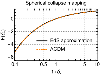
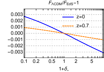
Let us take a closer look at the various ingredients that define the saddle-point configuration. We start with the function $F(\delta_{*})$. It is determined exclusively by the dynamics of spherical collapse and does not depend at all on the statistical properties of the perturbations. We have computed it using the procedure described in Appendix C for the cases of an EdS universe ($\Omega_{m}=1,\Omega_{\Lambda}=0$) and the reference $\Lambda$CDM cosmology ($\Omega_{m}=0.26,\Omega_{\Lambda}=0.74$). The results are shown in Fig. 1, left panel. The dependence on cosmology is very weak, so that the curves essentially overlay. In the EdS case the mapping is redshift-independent. Its behavior for small values of the argument is,

$$F_{\rm EdS}(\delta_{*})=\delta_{*}-\frac{17}{21}\delta_{*}^{2}+\frac{2815}{3969}\delta_{*}^{3}+{\cal O}(\delta_{*}^{4})\;,$$ (2.31a)

whereas its asymptotics at large over/underdensities are

$$F_{\rm EdS}\to 1.686 \text{at}\quad\delta_{*}\to\infty\,,$$ (2.31b)

$$F_{\rm EdS}\sim-(1+\delta_{*})^{-3/2} \text{at}\quad\delta_{*}\to-1\,.$$ (2.31c)

For $\Lambda$CDM this function has a very mild redshift dependence illustrated in the right panel of Fig. 1, which shows the relative difference between $F_{\Lambda{\rm CDM}}$ and $F_{\rm EdS}$. This difference is maximal for $z=0$, where it reaches a few per mil at the edges of the considered range of $\delta_{*}$. However, $F$ enters in the exponent of the PDF (see (2.30)) and a few per mil inaccuracy in it would generate a few percent relative error at the tails of the PDF. For these reasons we will use the exact $\Lambda$CDM mapping whenever the function $F$ appears in the leading exponent. In all other instances the EdS approximation provides sufficient accuracy.

Figure 2: Left panel: the saddle point linear density variance as a function of the final density in the cell at $z=0$ for comoving cell radii $10$ Mpc/$h$ and $15$ Mpc/$h$. Right panel: the dependence of the linear growth factor on redhsift in $\Lambda$CDM and EdS cosmologies. In the latter case, it is equal to $(1+z)^{-1}$.

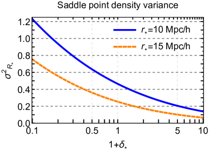
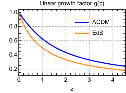
The second ingredient is the linear density variance at redshift zero $\sigma^{2}_{R_{*}}$. In contrast to $F$, it is determined only by the linear power spectrum and is independent of the non-linear dynamics. As already pointed out, it depends on the argument $\delta_{*}$ of the PDF through the Lagrangian radius $R_{*}$. This dependence is shown in the left panel of Fig. 2 for two different cell radii. By definition, $\sigma^{2}_{R_{*}}$ is independent of the redshift. The redshift dependence of the PDF comes through the linear growth factor $g$, shown as a function of $z$ in the right panel of Fig. 2. From the way $g^{2}$ and $\sigma^{2}_{R_{*}}$ enter the leading exponent (2.30) it is clear that the physical expansion parameter controlling the validity of the saddle-point approximation is the $z$-dependent linear variance $g^{2}(z)\sigma^{2}_{R_{*}}$. One expects the semiclassical expansion to work as long as $g^{2}\sigma^{2}_{R_{*}}\lesssim 1$. The numerical values of the linear density variance for $\delta_{*}=0$ are given in Table 1.

	$r_{*}=10$ Mpc$/h$	$r_{*}=15$ Mpc$/h$
z=0	0.464	0.254
z=0.7	0.238	0.130
z=4	0.0325	0.0177

Table 1: The filtered density variance $g^{2}\sigma^{2}_{r_{*}}$ for various redshifts and cell radii.

Figure 3: The saddle-point Lagrange multiplier, Eq. (2.29), as a function of $\delta_{*}$. The computation is performed in the EdS approximation.

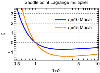
The Lagrange multiplier $\hat{\lambda}$ does not appear in the leading exponent of the PDF. However, we will see below that it enters the prefactor. So, it is instructive to plot its dependence on $\delta_{*}$, see Fig. 3. Note that it is positive (negative) for under- (over-) densities. It quickly grows at $\delta_{*}<0$.

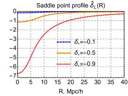
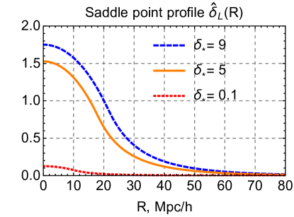
For completeness, we also present in Fig. 4 the saddle-point linear density profiles for several values of $\delta_{*}$. For $\delta_{*}\gtrsim 7$ the density profile in the central region exceeds the critical value $1.674$, and therefore the innermost part of the profile experiences shell-crossing. Conservatively, one would expect a breakdown of our saddle-point expansion for such large overdensities. However, we will see shortly that the available data are consistent with the semiclassical scaling even for $\delta_{*}\gtrsim 7$. This robustness of the semiclassical approach may be explained by the fact that the averaged density at $R_{*}$ is still less than the critical value even when the central regions undergo shell-crossing. Since the velocities of matter particles are rather low, it takes a significant amount of time for the information about shell-crossing to propagate to the boundary $R_{*}$. Until this happens, the dynamics of the boundary remain the same as if no shell-crossing occurred, so that the spherical collapse mapping used in the derivation of (2.30) still applies.

It should be stressed that having a spherical collapse saddle point does not mean that an exact spherical collapse happens inside each cell. Recall that in the case of tunneling in quantum mechanics the saddle-point solution, by itself, has measure zero in the space of all possible trajectories in the path integral, and thus is never realized precisely (see e.g. [54, 55]). What makes the tunneling amplitude finite are small perturbations around the saddle point solution that add up coherently and eventually contribute to the prefactor. From this argument it is clear that fluctuations around the saddle point are crucial for the consistency of our path integral calculation. If the saddle-point approximation works, the actual dynamics of the density field inside each cell is spherical collapse perturbed by aspherical fluctuations.

Figure 4: The saddle point linear density profiles in Lagrangian position space for several values of $\delta_{*}$ corresponding to underdensities (left panel) and overdensities (right panel). The results are shown for the cell radius $r_{*}=10$ Mpc$/h$.

2.3 Prefactor from fluctuations

We now consider small fluctuations around the spherical collapse saddle point found in the previous subsection. To leading order in $g^{2}$, the path integral over these fluctuations is Gaussian and produces the prefactor in front of the leading exponent (2.30), as was pointed out in Refs. [35, 36]. It is natural to expand the fluctuations of the linear density field in spherical harmonics. We write,

$$\delta_{L}({\bf k})=\hat{\delta}_{L}(k)+\delta_{L,0}^{(1)}(k)+\sum_{\ell>0}\sum_{m=-\ell}^{\ell}(-i)^{\ell}\,\delta_{L,\ell m}^{(1)}(k)\,Y_{\ell m}({\bf k}/k)\;,$$ (2.32a)

$$\lambda=\hat{\lambda}+\lambda^{(1)}\;,$$ (2.32b)

where we have singled out the monopole fluctuation $\delta_{L,0}^{(1)}$. Note that due to our convention for the spherical harmonics (see Appendix A), the reality condition $\big{(}\delta_{L}({\bf k})\big{)}^{*}=\delta_{L}(-{\bf k})$ translates into the conditions

$$\big{(}\delta_{L,0}^{(1)}(k)\big{)}^{*}=\delta_{L,0}^{(1)}(k)~{},~{}~{}~{}~{}\big{(}\delta_{L,\ell m}^{(1)}(k)\big{)}^{*}=\delta_{L,\ell,-m}^{(1)}(k)\;.$$ (2.33)

Fluctuations give rise to a perturbation of the averaged density contrast which up to second order can be written as,

$$\begin{split}\bar{\delta}_{W}=&\delta_{*}+\int[dk]\,4\pi S(k)\,\delta_{L,0}^{(1)}(k)+\int[dk]^{2}\,4\pi Q_{0}(k_{1},k_{2})\,\delta_{L,0}^{(1)}(k_{1})\delta_{L,0}^{(1)}(k_{2})\\ &+\sum_{\ell>0,m}\int[dk]^{2}\,Q_{\ell}(k_{1},k_{2})\,\delta_{L,\ell m}^{(1)}(k_{1})\delta^{(1)}_{L,\ell,-m}(k_{2})\;,\end{split}$$ (2.34)

where we introduced the notation,

$$[dk]^{n}\equiv\prod_{i=1}^{n}\frac{k^{2}_{i}dk_{i}}{(2\pi)^{3}}\;,$$ (2.35)

and $S$, $Q_{0}$, $Q_{\ell}$ are some kernels. Below we will refer to $Q_{0}$, $Q_{\ell}$ as response matrices. Note the factor $4\pi$ that we included in the definition of $S$ and $Q_{0}$; it reflects the difference in our normalization of spherical harmonics in the monopole and higher multipole sectors, see Eq. (A.8). In the expression (2.34) we have used the fact that non-monopole fluctuations can contribute only at quadratic order due to spherical symmetry. For the same reason, the kernels $Q_{\ell}$ do not depend on the azimuthal number $m$.

Substituting (2.32a) and (2.34) into the path integral (2.7), after a straightforward calculation, we find that the Gaussian integrals over fluctuations with different multipole numbers $\ell$ factorize. This leads to the following representation for the PDF,

$$\mathcal{P}(\delta_{*})={\cal A}_{0}\cdot\prod_{\ell>0}{\cal A}_{\ell}(\delta_{*})\cdot\exp\left\{-\frac{F^{2}(\delta_{*})}{2g^{2}\sigma^{2}_{R_{*}}}\right\}\,,$$ (2.36)

where

$${\cal A}_{0}= {\cal N}_{0}^{-1}\int_{-i\infty}^{i\infty}\frac{d\lambda^{(1)}}{2\pi ig^{2}}\int\mathscr{D}\delta_{L,0}^{(1)}\,\exp\bigg{\{}-\frac{4\pi}{g^{2}}\bigg{[}\int\frac{[dk]}{2P(k)}\big{(}\delta_{L,0}^{(1)}(k)\big{)}^{2}$$

$$\qquad+\lambda^{(1)}\int[dk]\,S(k)\,\delta_{L,0}^{(1)}(k)+\hat{\lambda}\int[dk]^{2}\,Q_{0}(k_{1},k_{2})\,\delta_{L,0}^{(1)}(k_{1})\delta_{L,0}^{(1)}(k_{2})\bigg{]}\bigg{\}}\;,$$ (2.37)

$${\cal A}_{\ell}= {\cal N}_{\ell}^{-1}\int[\mathscr{D}\delta_{L,lm}^{(1)}]\,\exp\bigg{\{}-\frac{1}{g^{2}}\sum_{m}\bigg{[}\int\frac{[dk]}{2P(k)}\delta_{L,\ell m}^{(1)}(k)\delta_{L,\ell,-m}^{(1)}(k)$$

$$\qquad\qquad\qquad\qquad\qquad+\hat{\lambda}\int[dk]^{2}\,Q_{\ell}(k_{1},k_{2})\,\delta_{L,\ell m}^{(1)}(k_{1})\delta^{(1)}_{L,\ell,-m}(k_{2})\bigg{]}\bigg{\}}\;.$$ (2.38)

The integration measure in the last expression is $[\mathscr{D}\delta_{L,lm}^{(1)}]=\prod_{m=-l}^{l}\mathscr{D}\delta_{L,lm}^{(1)}$, whereas the normalization factors are,

$${\cal N}_{0}=\int\mathscr{D}\delta_{L,0}\,\exp\bigg{\{}-\frac{4\pi}{g^{2}}\int\frac{[dk]}{2P(k)}\big{(}\delta_{L,0}(k)\big{)}^{2}\bigg{\}}\;,$$ (2.39)

$${\cal N}_{\ell}=\int[\mathscr{D}\delta_{L,lm}]\,\exp\bigg{\{}-\frac{1}{g^{2}}\sum_{m}\int\frac{[dk]}{2P(k)}\delta_{L,\ell m}(k)\delta_{L,\ell,-m}(k)\bigg{\}}\;.$$ (2.40)

Despite appearing more complicated, the monopole prefactor ${\cal A}_{0}$ can be evaluated analytically. This is not surprising, since the dynamics in the monopole sector is known exactly. We postpone this analysis to the next section and focus here on the prefactor stemming from higher multipoles.

The quadratic form in the exponent of Eq. (2.38) is a convolution of the vector $\delta_{L,\ell m}^{(1)}$ with the matrix

$$\frac{1}{g^{2}}\bigg{(}\mathbb{1}\cdot\frac{1}{P(k)}+2\hat{\lambda}Q_{\ell}\bigg{)}\,\delta_{m,-m}\;,$$

where $\mathbb{1}$ is the unit operator in $k$-space whose kernel with respect to the measure (2.35) is,

$$\mathbb{1}(k,k^{\prime})=(2\pi)^{3}k^{-2}\delta_{\rm D}^{(1)}(k-k^{\prime})\;,$$ (2.41)

and $\delta_{m,-m}$ is the Kronecker symbol. The Gaussian integral over $\delta_{L,\ell m}^{(1)}$ is inversely proportional to the square root of the determinant of this matrix. To get ${\cal A}_{\ell}$, this determinant must be divided by the determinant of the corresponding matrix in the normalization factor (2.40) which is simply

$$\frac{1}{g^{2}}\bigg{(}\mathbb{1}\cdot\frac{1}{P(k)}\bigg{)}\,\delta_{m,-m}\;.$$

In this way we obtain

$${\cal A}_{\ell}=\mathcal{D}_{\ell}^{-(\ell+1/2)}\,,$$ (2.42)

where

$$\mathcal{D}_{\ell}=\det\left(\mathbb{1}+2\hat{\lambda}\sqrt{P}Q_{\ell}\sqrt{P}\right)\,,$$ (2.43)

is the $\ell$th aspherical fluctuation determinant. The second term in $\mathcal{D}_{\ell}$ denotes an operator with the kernel $\sqrt{P(k)}Q_{\ell}(k,k^{\prime})\sqrt{P(k^{\prime})}$. It is convenient to introduce the aspherical prefactor that aggregates contributions of all multipoles with strictly positive $\ell$,

$$\mathcal{A}_{\text{ASP}}\equiv\prod_{\ell>0}\mathcal{A}_{\ell}=\prod_{\ell>0}\mathcal{D}_{\ell}^{-(\ell+1/2)}\,.$$ (2.44)

We see that its computation requires knowledge of the aspherical response matrices $Q_{\ell}$.

Let us make an important remark. The growth factor $g$ has dropped out of the expression for the fluctuation determinants (2.43). Also, it can be shown that the response matrices $Q_{\ell}$ do not depend on the redshift (see Sec. 5). This implies that the aspherical prefactor is redshift-independent. We are going to see in the next section that this theoretical expectation is confirmed by the N-body data.

The redshift-independence of ${\cal A}_{\rm ASP}$ may be somewhat puzzling. Indeed, being a non-trivial function of $\delta_{*}$, the aspherical prefactor affects the shape of PDF even at early times, when the distribution must be Gaussian. To resolve this apparent paradox, we notice that at high redshifts (in the limit $g^{2}\to 0$) the distribution (2.36) approaches the delta-function centered at $\delta_{*}=0$. On the other hand, recall that $\hat{\lambda}$ vanishes at $\delta_{*}$ (see Fig. 3) and hence $\mathcal{D}_{\ell}(\delta_{*}=0)=1$ for all $\ell$. This implies ${\cal A}_{\text{ASP}}(\delta_{*}=0)=1$ and in the limit $g^{2}\to 0$ the whole aspherical prefactor reduces to unity. One concludes that the role of the aspherical prefactor decreases as the distribution becomes sharper towards high redshifts.

3 Closer look at the prefactor

In this section we explicitly compute the monopole prefactor ${\cal A}_{0}$ from the spherical collapse dynamics. We then use N-body data to extract the aspherical prefactor ${\cal A}_{\rm ASP}$ and discuss its main properties.

3.1 Monopole

The factorization property (2.36) implies that in the computation of the monopole prefactor all aspherical perturbations can be set to zero. Thereby it is convenient to consider the path integral over the spherically symmetric sector as a whole, without splitting the density field into the saddle-point configuration and fluctuations. In this way we arrive at what can be called ‘spherical PDF’,

$$\mathcal{P}_{\text{SP}}(\delta_{*})=\mathcal{N}_{0}^{-1}\int\mathscr{D}\delta_{L,0}\exp\bigg{\{}-\frac{4\pi}{g^{2}}\int\frac{[dk]}{2P(k)}\big{(}\delta_{L,0}(k)\big{)}^{2}\bigg{\}}\,\delta_{D}^{(1)}\big{(}\delta_{*}-\bar{\delta}_{W}[\delta_{L,0}]\big{)}\,,$$ (3.1)

with the normalization factor given in Eq. (2.39). We stress that ${\cal P}_{\rm SP}$ is not equal to the true PDF, as it restricts the original path integral (2.5) to spherically symmetric configurations only, and thus misses the contribution of aspherical modes.

Due to the existence of the spherical collapse mapping (2.14), the condition $\delta_{*}=\bar{\delta}_{W}[\delta_{L,0}]$ is equivalent to the condition $F(\delta_{*})=\bar{\delta}_{L,0}(R_{*})$. Thus, the delta-function in (3.1) is proportional to the delta-function of the argument $F(\delta_{*})-\bar{\delta}_{L,0}(R_{*})$,

$$\delta^{(1)}_{D}\big{(}\delta_{*}-\bar{\delta}_{W}[\delta_{L,0}]\big{)}=C[\delta_{L,0}]\cdot\delta^{(1)}_{D}\big{(}F(\delta_{*})-\bar{\delta}_{L,0}(R_{*})\big{)}\,.$$ (3.2)

The proportionality coefficient $C$ is given in Eq. (2.22); it is fixed by the requirement that the integral of both sides of (3.2) over $\delta_{*}$ produces unity. Substituting this relation into Eq. (3.1) and using the integral representation for the delta-function we obtain,

$$\begin{split}\mathcal{P}_{\text{SP}}(\delta_{*})=&\mathcal{N}_{0}^{-1}\int_{-i\infty}^{i\infty}\frac{d\lambda}{2\pi ig^{2}}\,{\rm e}^{\lambda F/g^{2}}\int\mathscr{D}\delta_{L,0}\,C[\delta_{L,0}]\\ &\times\exp\bigg{\{}-\frac{4\pi}{g^{2}}\bigg{[}\int\frac{[dk]}{2P(k)}\big{(}\delta_{L,0}(k)\big{)}^{2}+\lambda\int[dk]W_{\rm th}(kR_{*})\delta_{L,0}(k)\bigg{]}\bigg{\}}\,.\end{split}$$ (3.3)

It is now straightforward to evaluate this integral by the saddle point method, which yields,

$$\mathcal{P}_{\text{SP}}(\delta_{*})=\frac{\hat{C}(\delta_{*})}{\sqrt{2\pi g^{2}\sigma^{2}_{R_{*}}}}\exp\left(-\frac{F^{2}(\delta_{*})}{2g^{2}\sigma^{2}_{R_{*}}}\right)\,,$$ (3.4)

where $\hat{C}$ is defined in (2.29). From this expression we infer the monopole prefactor,

$${\cal A}_{0}(\delta_{*})=\frac{\hat{C}(\delta_{*})}{\sqrt{2\pi g^{2}\sigma^{2}_{R_{*}}}}\;.$$ (3.5)

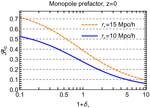
We plot its dependence on the density contrast in Fig. 5. It varies roughly by an order of magnitude in the range $\delta_{*}=[-0.9,9]$. Since it is inversely proportional to the r.m.s density contrast $g\sigma_{R_{*}}$, it significantly varies with the window function radius and redshift. For illustration purposes we show the results for $z=0$. The curves for other redshifts are qualitatively similar and can be obtained upon rescaling by an appropriate growth factor (shown in the right panel of Fig. 2).

Figure 5: The monopole prefactor at $z=0$.

By construction, the spherical PDF (3.1) is normalized to unity,

$$\int_{-1}^{\infty}d\delta_{*}\,\mathcal{P}_{\text{SP}}(\delta_{*})=1\,.$$ (3.6)

However, it does not reproduce the correct zero mean value of the density contrast,

$$\langle\delta_{*}\rangle_{\rm SP}\equiv\int_{-1}^{\infty}d\delta_{*}\,{\cal P}_{\rm SP}(\delta_{*})\,\delta_{*}\neq 0\;.$$ (3.7)

To see this, we define the variable $\nu=F/\sigma_{R_{*}}$ and rewrite (3.4) as

$${\cal P}_{\rm SP}=\frac{1}{\sqrt{2\pi g^{2}}}\,\frac{d\nu}{d\delta_{*}}\,{\rm e}^{-\frac{\nu^{2}}{2g^{2}}}\;.$$ (3.8)

The expectation value (3.7) becomes,

$$\langle\delta_{*}\rangle_{\rm SP}=\int_{-\infty}^{\infty}\frac{d\nu}{\sqrt{2\pi g^{2}}}\,\delta_{*}(\nu)\,{\rm e}^{-\frac{\nu^{2}}{2g^{2}}}=\frac{g^{2}}{2}\frac{d^{2}\delta_{*}}{d\nu^{2}}\bigg{|}_{\nu=0}\;,$$ (3.9)

where we have evaluated the integral at leading order in $g^{2}$. It is straightforward to compute the second derivative appearing in the above equation. One finds,

$$\frac{d^{2}\delta_{*}}{d\nu^{2}}\bigg{|}_{\nu=0}=-\sigma_{r_{*}}^{2}\bigg{[}F^{\prime\prime}(0)+2\bigg{(}1-\frac{\xi_{r_{*}}}{\sigma^{2}_{r_{*}}}\bigg{)}\bigg{]}\;.$$ (3.10)

Using also the Taylor expansion (2.31a) for the function $F$ one obtains,

$$\langle\delta_{*}\rangle_{\rm SP}=-g^{2}\sigma_{r_{*}}^{2}a_{1}\,,~{}~{}~{}~{}~{}~{}\text{where}~{}~{}a_{1}=\frac{4}{21}-\frac{\xi_{r_{*}}}{\sigma^{2}_{r_{*}}}\;.$$ (3.11)

The numerical values of $a_{1}$ for different cell radii are given in Table 2 in the next subsection.

At first sight, the fact that the spherical PDF fails to reproduce the zero mean value of $\delta_{*}$ may seem surprising. However, it becomes less so once we realize that vanishing of $\langle\delta_{*}\rangle$ is related to translational invariance. Indeed, it is implied by the vanishing of $\langle\delta({\bf x})\rangle$, the mean density contrast at each space point. The latter, in turn, involves two ingredients: (i) the constraint $\int d^{3}x\,\delta({\bf x})=0$ which follows trivially from the definition of the density contrast, and (ii) the fact that, due to translational invariance, $\langle\delta({\bf x})\rangle$ is the same at all points. But the translational invariance has been explicitly broken by the reduction of the path integral to the spherically symmetric sector that singles out the origin as a preferred point in space. The correct identity $\langle\delta_{*}\rangle=0$ will be restored once we take into account the aspherical prefactor generated by fluctuations beyond the monopole sector.

3.2 Aspherical prefactor from N-body data

Figure 6: 1-point PDF of the smoothed density field at redshift $z=0$ for $r_{*}=10$ Mpc/$h$ (left panel) and $r_{*}=15$ Mpc/$h$ (right panel): the spherical PDF given by Eq. (3.4) (blue line) against the N-body data (black dots). Error-bars on the data points show the statistical uncertainty.

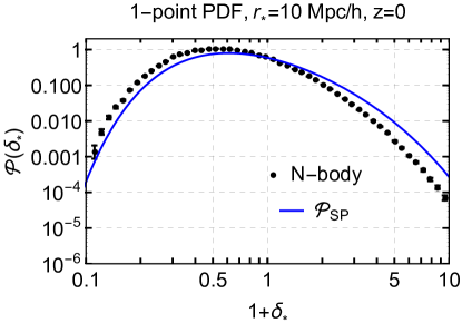
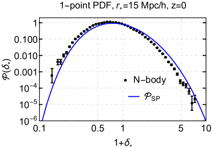
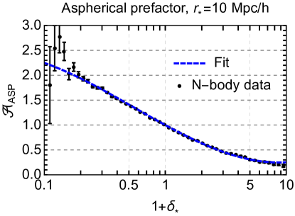
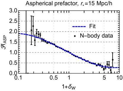
Before delving into the calculation of the aspherical prefactor, let us verify the semiclassical factorization formula (2.36) against the N-body data. To this end, we have run a suite of N-body simulations using the FastPM code [51] and obtained the counts-in-cells statistics for a total of $518400$ cells with radius $r_{*}=10$ Mpc$/h$ and $153600$ cells with $r_{*}=15$ Mpc$/h$. The details of our simulations are presented in Appendix B. Figure 6 shows the data points together with the spherical PDF ${\cal P}_{\rm SP}$. The results are shown for redshift $z=0$. The PDFs for other redshifts are qualitatively similar and will be discussed shortly. From Fig. 6 we see that although the spherical PDF correctly captures the exponential falloff of the data points at large over-/under-densities, it is clearly off-set from the data even at $\delta_{*}=0$. According to (2.36), this off-set should be compensated by the aspherical prefactor ${\cal A}_{\text{ASP}}$. Using the full PDF $\mathcal{P}_{\rm data}(\delta_{*})$ measured from the data, we can extract the aspherical prefactor as

$${\cal A}_{\rm ASP}(\delta_{*})=\frac{{\cal P}_{\rm data}(\delta_{*})}{{\cal P}_{\rm SP}(\delta_{*})}\;.$$ (3.12)

The result is shown in Fig. 7 for various redshifts and cell radii. At higher redshifts the distribution becomes sharper, which increases the measurement errors away from the origin. This is especially visible in the case $z=4$ where the available $\delta_{*}$-range in the data significantly shrinks compared to $z=0$. The errorbars shown in the plots represent the statistical uncertainty of our data. It is worth noting that the bins at the tails of the distribution are expected to contain also a systematic error comparable to the statistical one, see the discussion in Appendix B.

Figure 7: The aspherical prefactor ${\cal A}_{\text{ASP}}=\mathcal{P}_{\rm data}/\mathcal{P}_{\text{SP}}$ extracted from the simulations. The results are shown for the cell radii 10 Mpc/$h$ (left panel) and 15 Mpc/$h$ (right panel).

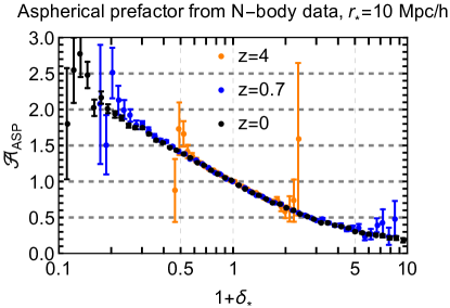
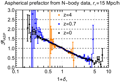
The spherical PDF has an exponential sensitivity to the density variance, which changes by an order of magnitude across the considered redshifts, see Tab. 1. Similarly, the measured PDF’s at different redshifts and cell radii are exponentially different. Nevertheless, we observe that the results of their division by the spherical PDF’s depend very weakly on the redshift and the size of the window function. This is a strong confirmation of the validity of the semiclassical scaling (2.36). In particular, we conclude that the spherical collapse saddle point indeed dominates the probability: if it were not the case, one would expect exponentially large difference between ${\cal P}_{\rm data}$ and ${\cal P}_{\rm SP}$. Moreover, the data are clearly consistent with the redshift-independence of ${\cal A}_{\rm ASP}$, as predicted by the theory (see Sec. 2.3). Note that the aspherical prefactor is a very smooth function that varies only by an order of magnitude within the density range where the whole PDF varies by six-seven orders of magnitude.

In complete agreement with the theoretical expectation (recall the discussion at the end of Sec. 2.3), we see that ${\cal A}_{\rm ASP}\big{|}_{\delta_{*}=0}=1$. Note that this ensures the correct normalization of the full PDF ${\cal P}={\cal A}_{\rm ASP}\mathcal{P}_{\rm SP}$ in the leading semiclassical approximation. Indeed, in this approximation the PDF is concentrated around $\delta_{*}=0$ and we have,

$$\int d\delta_{*}\,{\cal A}_{\rm ASP}(\delta_{*})\mathcal{P}_{\rm SP}(\delta_{*})={\cal A}_{\rm ASP}\big{|}_{\delta_{*}=0}\int d\delta_{*}\,\mathcal{P}_{\rm SP}(\delta_{*})={\cal A}_{\rm ASP}\big{|}_{\delta_{*}=0}\;.$$

Let us now see how inclusion of the aspherical prefactor restores the zero expectation value of the density contrast. To this end, we introduce the variable $\nu$ as in (3.8) and write,

$$\begin{split}\langle\delta_{*}\rangle&=\int_{-1}^{\infty}d\delta_{*}\,{\cal A}_{\rm ASP}(\delta_{*})\mathcal{P}_{\rm SP}(\delta_{*})\,\delta_{*}=\int_{-\infty}^{\infty}\frac{d\nu}{\sqrt{2\pi g^{2}}}\,{\cal A}_{\text{ASP}}(\nu)\,\delta_{*}(\nu)\,{\rm e}^{-\frac{\nu^{2}}{2g^{2}}}\\ &=g^{2}\bigg{(}\frac{d{\cal A}_{\rm ASP}}{d\nu}\cdot\frac{d\delta_{*}}{d\nu}+\frac{1}{2}\frac{d^{2}\delta_{*}}{d\nu^{2}}\bigg{)}\bigg{|}_{\nu=0}\;,\end{split}$$ (3.13)

where in the last equality we evaluated the integral at leading order in $g^{2}$. For $\langle\delta_{*}\rangle$ to vanish, the first derivative of ${\cal A}_{\rm ASP}$ at $\delta_{*}=0$ must satisfy,

$$\frac{d{\cal A}_{\rm ASP}}{d\delta_{*}}\bigg{|}_{\delta_{*}=0}=-\frac{1}{2}\bigg{(}\frac{d\delta_{*}}{d\nu}\bigg{)}^{-2}\frac{d^{2}\delta_{*}}{d\nu^{2}}\bigg{|}_{\nu=0}\;.$$

Comparing with Eq. (3.10) we obtain the condition

$$\frac{d{\cal A}_{\rm ASP}}{d\delta_{*}}\bigg{|}_{\delta_{*}=0}=a_{1}\;,$$ (3.14)

where $a_{1}$ has been defined in (3.11).

We have checked that the N-body data are fully consistent with this requirement. Namely, we fit the dependence ${\cal A}_{\rm ASP}(\delta_{*})$ extracted from the data with the formula

$$\begin{split}{\cal A}_{\text{ASP}}&=1+a_{1}\mathop{\rm ln}\nolimits(1+\delta_{*})+a_{2}\mathop{\rm ln}\nolimits^{2}(1+\delta_{*})+a_{3}\mathop{\rm ln}\nolimits^{3}(1+\delta_{*})\,,\end{split}$$ (3.15)

where we fix $a_{1}$ to the numerical values predicted by Eq. (3.11), whereas $a_{2}$ and $a_{3}$ are treated as free parameters of the fit. The results of the fit are shown in Fig. 8 and the parameters are summarized in Table 2. We observe that the expression (3.15) accurately describes the data throughout the whole available range of densities. In particular, there is a perfect match between the slopes of the fitting curve and the data at the origin. Note that the precise values of the coefficients $a_{2}$, $a_{3}$ listed in Table 2 should be taken with a grain of salt as they are determined by the tails of the measured distribution, which are subject to systematic errors.

Figure 8: The fitting formula for the aspherical prefactor (3.15) against the N-body data for $r_{*}=10$ Mpc$/h$ (left panel) and $r_{*}=15$ Mpc$/h$ (right panel). All results are shown for $z=0$.

	$a_{1}$	$a_{2}$	$a_{3}$
$r_{*}=10$ Mpc$/h$	$-0.575$	$~{}0.047~{}$	$~{}0.027~{}$
$r_{*}=15$ Mpc$/h$	$-0.546$	$~{}0.018~{}$	$~{}0.037~{}$

Table 2: Parameters of the fitting formula (3.15) for the aspherical prefactor for two different cell radii. The parameter $a_{1}$ is computed from Eq. (3.11), and is not fitted from the data.

We have seen that the aspherical prefactor is independent of the linear growth factor. We also observe that the prefactor depends rather weakly on the size of the window function. The leading response of the PDF to a change in the cosmological model (such as e.g. variation of the cosmological parameters or beyond-$\Lambda$CDM physics) will clearly enter through the exponent of the spherical part ${\cal P}_{\rm SP}$. The modification of the PDF due to the change of ${\cal A}_{\rm ASP}$ is expected to be subdominant. Hence, for practical applications of the 1-point PDF to constraining the cosmological parameters or exploring new physics one can, in principle, proceed with the simple fitting formula (3.15) with the parameters extracted from N-body simulations of a fiducial $\Lambda$CDM cosmology.

Nevertheless, from the theoretical perspective, it is highly instructive to perform the full first-principle calculation of the aspherical prefactor. The rest of the paper is devoted to this task. In the four subsequent sections we derive and analyze the relevant equations. A reader interested in the final results can jump directly to Sec. 8.

4 Perturbative calculation at small density contrast

In this section we compute the aspherical prefactor treating the saddle point configuration perturbatively. This approximation is valid at small contrasts $|\delta_{*}|\ll 1$. We will work at quadratic order in $\delta_{*}$ which, as we will see shortly, corresponds to the 1-loop order of standard perturbation theory. We first consider standard cosmological perturbation theory (SPT) [2] and then discuss its extension, the effective field theory (EFT) of large scale structure [14, 15]. Eventually, we are interested in large averaged density contrasts $|\delta_{*}|\sim 1$ where perturbation theory does not apply. Still, it will serve us to grasp important features of a fully non-linear calculation.

It is convenient to introduce an alternative representation of the aspherical prefactor. Let us multiply and divide the expression (2.44) by the square root of the monopole fluctuation determinant

$$\mathcal{D}_{0}=\text{det}\left[\mathbb{1}+2\hat{\lambda}\sqrt{P}Q_{0}\sqrt{P}\right]\,,$$ (4.1)

where $Q_{0}$ is the monopole response matrix introduced in (2.34). Next we observe that

$$\begin{split}\prod_{\ell=0}^{\infty}{\cal D}_{\ell}^{-(\ell+1/2)}={\cal N}^{-1}\int&\mathscr{D}\delta_{L}^{(1)}\exp\bigg{\{}-\frac{1}{g^{2}}\bigg{[}\int_{{\bf k}}\frac{\big{(}\delta_{L}^{(1)}({\bf k})\big{)}^{2}}{2P(k)}\\ &+\hat{\lambda}\int_{{\bf k}_{1}}\int_{{\bf k}_{2}}Q_{tot}({\bf k}_{1},{\bf k}_{2})\,\delta_{L}^{(1)}({\bf k}_{1})\,\delta_{L}^{(1)}({\bf k}_{2})\bigg{]}\bigg{\}}\,,\end{split}$$ (4.2)

where

$$Q_{tot}({\bf k}_{1},{\bf k}_{2})=\frac{1}{2}\frac{\partial^{2}\bar{\delta}_{W}}{\partial\delta_{L}({\bf k}_{1})\partial\delta_{L}({\bf k}_{2})}\,$$ (4.3)

is the total quadratic response operator. Note that it is defined in the space of functions depending on the full 3-dimensional wavevectors ${\bf k}$, unlike the partial multipole operators $Q_{\ell}$ defined in the space of functions of the radial wavenumber $k$. The expression on the r.h.s. of (4.2) is the inverse square root of the total fluctuation determinant,

$$\mathcal{D}_{tot}=\text{det}[\mathbb{1}+2\hat{\lambda}\sqrt{P}Q_{tot}\sqrt{P}]\,.$$ (4.4)

In this way we obtain the following formula for the aspherical prefactor,

$$\mathcal{A}_{\text{ASP}}=\sqrt{\frac{\mathcal{D}_{0}}{{\mathcal{D}_{tot}}}}\,.$$ (4.5)

The monopole determinant ${\cal D}_{0}$ can be computed analytically for any value of $\delta_{*}$, see Appendix C.3. Note that, by itself, it does not have any physical meaning as the quadratic monopole fluctuations are already taken into account in the monopole prefactor ${\cal A}_{0}$. The introduction of the monopole determinant is just a useful trick to simplify the calculation, ${\cal D}_{tot}$ being more convenient to treat in perturbation theory than the determinants in separate multipole sectors.

4.1 Fluctuation determinant in standard perturbation theory

In order to find the response matrix we use the SPT solution [2] for the mildly non-linear density field,

$$\delta({\bf k})=\delta_{L}({\bf k})+\sum_{n=2}^{\infty}\int_{{\bf k}_{1}}...\int_{{\bf k}_{n}}(2\pi)^{3}\delta^{(3)}_{D}\Big{(}{\bf k}-\sum_{i}{\bf k}_{i}\Big{)}F_{n}({\bf k}_{1},...,{\bf k}_{n})\prod_{i=1}^{n}\delta_{L}({\bf k}_{i})\,.$$ (4.6)

We work in the EdS approximation, where the SPT kernels $F_{n}$ are redshift-independent, e.g.

$$F_{2}({\bf k}_{1},{\bf k}_{2})=\frac{17}{21}+({\bf k}_{1}\cdot{\bf k}_{2})\left(\frac{1}{2k_{1}^{2}}+\frac{1}{2k_{2}^{2}}\right)+\frac{2}{7}\left(\frac{({\bf k}_{1}\cdot{\bf k}_{2})^{2}}{k_{1}^{2}k_{2}^{2}}-\frac{1}{3}\right)\,.$$ (4.7)

We will discuss the EFT corrections later on. Using (4.6) we obtain

$$\begin{split}Q_{tot}({\bf k}_{1},{\bf k}_{2})=\sum_{n=2}^{\infty}\frac{n(n-1)}{2}\int_{{\bf q}_{1}}...\int_{{\bf q}_{n-2}}&F_{n}({\bf k}_{1},{\bf k}_{2},{\bf q}_{1},...,{\bf q}_{n-2})\\ &\times W_{\rm th}(|{\bf k}_{12}+{\bf q}_{1...n-2}|r_{*})\prod_{i=1}^{n-2}\hat{\delta}_{L}({\bf q}_{i})\,,\end{split}$$ (4.8)

where ${\bf q}_{1...m}\equiv{\bf q}_{1}+...+{\bf q}_{m}$. We will keep only the first two terms in the expansion (4.8):

$$Q_{tot}({\bf k}_{1},{\bf k}_{2})=F_{2}({\bf k}_{1},{\bf k}_{2})\,W_{\rm th}(|{\bf k}_{12}|r_{*})+3\int_{{\bf q}}F_{3}({\bf k}_{1},{\bf k}_{2},{\bf q})\,W_{\rm th}(|{\bf k}_{12}+{\bf q}|r_{*})\,\hat{\delta}_{L}({\bf q})\,.$$ (4.9)

An important comment is in order. The SPT kernels $F_{n}({\bf k}_{1},...,{\bf k}_{n})$ are known to contain poles when one or several momenta vanish, see e.g. the second term in (4.7). These lead to the so-called ‘IR divergence’ in the individual SPT loop integrals that cancel in the final results for the correlation functions [3]. Equation (4.9) implies that the response matrix has IR poles when ${\bf k}_{1}$ or ${\bf k}_{2}$ (or both) tend to zero. Nevertheless, we are going to see that the IR divergences associated with these poles cancel in the determinant ${\cal D}_{tot}$. In other words, the aspherical prefactor, and hence the full 1-point PDF, is IR safe. In Sec. 6.1 this property will be related to the equivalence principle.

To compute the determinant ${\cal D}_{tot}$, we make use of the trace formula,

$$\begin{split}\mathcal{D}_{tot}&=\exp\left\{\text{Tr}\mathop{\rm ln}\nolimits\left(\mathbb{1}+2\hat{\lambda}\sqrt{P}Q_{tot}\sqrt{P}\right)\right\}\\ &\approx\exp\left\{\left[-2\frac{\delta_{*}}{\sigma^{2}_{r_{*}}}+6\frac{\delta_{*}^{2}}{\sigma^{2}_{r_{*}}}\left(-\frac{4}{21}+\frac{\xi_{r_{*}}}{\sigma^{2}_{r_{*}}}\right)\right]\text{Tr}(PQ_{tot})-2\frac{\delta_{*}^{2}}{\sigma_{r_{*}}^{4}}\text{Tr}(PQ_{tot}PQ_{tot})\right\}\,,\end{split}$$ (4.10)

where in the second line we perturbatively expanded the Lagrange multiplier $\hat{\lambda}$ and kept only the terms that can contribute at order $\delta_{*}^{2}$. Let us first compute the leading-order contribution $O(\delta_{*})$. From Eq. (4.9) it is proportional to

$$\begin{split}\text{Tr}(Q_{tot}P)_{\text{LO}}=W_{\rm th}(0)\int_{{\bf k}}\,F_{2}({\bf k},-{\bf k})P(k)\,.\end{split}$$ (4.11)

But this vanishes due to $F_{2}({\bf k},-{\bf k})=0$. Note that this property can be traced back to the translational invariance. Indeed, the latter implies conservation of momentum, so that at quadratic order of SPT around homogeneous background one has,

$$\delta({\bf k})=\delta_{L}({\bf k})+\int_{\bf q}F_{2}({\bf k}-{\bf q},{\bf q})\,\delta_{L}({\bf k}-{\bf q})\delta_{L}({\bf q})\;.$$

Averaging over the Gaussian initial conditions and recalling that $\langle\delta({\bf k})\rangle=\langle\delta_{L}({\bf k})\rangle=0$ by construction, one obtains that the integral entering (4.11) must vanish. As this should be true for any power spectrum, one further infers vanishing of $F_{2}({\bf k},-{\bf k})$.

At next-to-leading order one has,

$$\text{Tr}(Q_{tot}P)_{\text{NLO}}=3\frac{\delta_{*}}{\sigma^{2}_{r_{*}}}\int_{{\bf k}}\int_{{\bf q}}F_{3}({\bf q},-{\bf q},{\bf k})P(k)P(q)|W_{\rm th}(kr_{*})|^{2}\,.$$ (4.12)

This term is similar to the $P_{13}$-contribution to the filtered density variance in SPT. It is known to contain a spurious IR-enhancement, which cancels upon adding the $P_{22}$ contribution, whose counterpart in our calculation is the rightmost term in (4.10),

$$\text{Tr}(Q_{tot}PQ_{tot}P)=\int_{{\bf k}_{1}}\int_{{\bf k}_{2}}F_{2}^{2}({\bf k}_{1},{\bf k}_{2})P(k_{1})P(k_{2})\big{|}W_{\rm th}(|{\bf k}_{1}+{\bf k}_{2}|r_{*})\big{|}^{2}\,.$$ (4.13)

The net expression for the prefactor generated by total fluctuations reads:

$$\mathcal{A}_{tot}\equiv\mathcal{D}_{tot}^{-1/2}\approx\exp\left\{\frac{\delta_{*}^{2}}{2}\frac{\sigma^{2}_{\text{1-loop}}}{\sigma^{4}_{r_{*}}}\right\}\,,$$ (4.14)

where we defined the filtered 1-loop density variance:

$$\sigma^{2}_{\text{1-loop}}=\int_{\bf k}P_{\text{1-loop}}(k)|W_{\rm th}(kr_{*})|^{2}\;,$$ (4.15a)

$$P_{\text{1-loop}}(k)=\int_{\bf q}\Big{(}2F_{2}^{2}({\bf k}-{\bf q},{\bf q})P(q)P(|{\bf k}-{\bf q}|)+6F_{3}({\bf k},-{\bf q},{\bf q})P(q)P(k)\Big{)}\,.$$ (4.15b)

This result has an intuitive interpretation. One can get expression (4.14) by replacing the linear matter power spectrum in the density variance of the saddle-point exponent (2.30) by its 1-loop version,

$$\exp\left\{-\frac{\delta_{*}^{2}}{2g^{2}(\sigma^{2}_{r_{*}}+g^{2}\sigma^{2}_{\text{1-loop}})}\right\}\approx\exp\left\{-\frac{\delta_{*}^{2}}{2g^{2}\sigma^{2}_{r_{*}}}+\frac{\delta_{*}^{2}}{2}\frac{\sigma_{\text{1-loop}}^{2}}{\sigma^{4}_{r_{*}}}\right\}\,.$$ (4.16)

The replacement of the linear variance by the 1-loop expression in (4.16) is reminiscent of the coupling constant renormalization due to radiative corrections in instanton calculations in QFT (see e.g. [56]).

4.2 Effective field theory corrections

SPT does not capture correctly the effect of very short modes that become deeply non-linear by $z=0$. This problem is addressed in EFT of LSS. The latter augments the pressureless hydrodynamics equations solved in SPT by the effective stress tensor, which is treated within a gradient expansion [14, 15, 17]. At the leading (1-loop) order it produces the following correction (counterterm) to the density contrast,

$$\delta_{\text{ctr}}({\bf k})=-\gamma(z)k^{2}\delta_{L}({\bf k})\,,$$ (4.17)

which must be added to the SPT expression (4.6). Here $\gamma(z)$ is a $z$-dependent coefficient with the dimension of (length)² whose value and scaling with $g(z)$ will be discussed below. Note that this contribution is linear in $\delta_{L}$. However, it has the same order of magnitude as the one-loop correction because the combination $\gamma k^{2}$ is assumed to be small according to the rules of gradient expansion.

Addition of the term (4.17) to the relation between linear and non-linear density contrasts slightly modifies the saddle-point solution. To find this correction we observe that, at the order we are working, the final smoothed density contrast is related to the linear density field as,

$$\bar{\delta}_{W}=\int_{\bf k}W_{\rm th}(kr_{*})\,\delta_{L}({\bf k})\,(1-\gamma k^{2}).$$ (4.18)

Substituting this into the saddle-point equations (2.9) we obtain,

$$\hat{\delta}_{L}=\frac{\delta_{*}}{\sigma^{2}_{r_{*}}}\bigg{(}1+\frac{2\gamma\Sigma^{2}_{r_{*}}}{\sigma_{r_{*}}^{2}}\bigg{)}P(k)W_{\rm th}(kr_{*})(1-\gamma k^{2})\;,$$ (4.19)

where

$$\Sigma^{2}_{r_{*}}=\int_{\bf k}|W_{\rm th}(kr_{*})|^{2}\,P(k)\,k^{2}\;.$$ (4.20)

The modification of the saddle point produces a shift in the leading exponent of the PDF and results in the following counterterm prefactor:

$${\cal A}_{\text{ctr}}=\exp\left(-\delta_{*}^{2}\frac{\gamma(z)}{g^{2}(z)}\frac{\Sigma_{r_{*}}^{2}}{\sigma^{4}_{r_{*}}}\right)\,.$$ (4.21)

It is instructive to derive this result in an alternative way. One recalls that the 1-loop SPT correction to the power spectrum (4.15b) receives a large contribution from short modes that has the form (see e.g. [17]),

$$g^{2}P_{\text{1-loop, UV}}(k)=\bigg{(}-\frac{61}{630\pi^{2}}\int_{q\gg k}dqP(q)\bigg{)}g^{2}k^{2}P(k)\;.$$ (4.22)

This contributons would be divergent for a universe where the spectrum $P(q)$ falls slower than $q^{-1}$ at $q\to\infty$. In EFT of LSS it is renormalized by the counterterm $-2\gamma k^{2}P(k)$ coming from the correction (4.17). Performing the renormalization inside the filtered 1-loop density variance we obtain the expression,

$$\sigma_{\text{1-loop, ren}}^{2}=\sigma_{\text{1-loop}}^{2}-\frac{2\gamma}{g^{2}}\Sigma^{2}_{r_{*}}\;,$$ (4.23)

which translates into the multiplication of the 1-loop prefactor ${\cal A}_{tot}$ by the counterterm (4.21).

We obtain the value of the EFT coefficient $\gamma(z=0)$ by fitting the dark matter power spectrum of the simulations at $z=0$ to the 1-loop IR-resummed theoretical template of [12]. We follow Ref. [19] to include the theoretical error in our analysis, which yields the following result:

$$\gamma_{0}\equiv\gamma\big{|}_{z=0}=1.51\pm 0.07\quad(\text{Mpc}/h)^{2}\,.$$ (4.24)

In general, the redshift dependence of $\gamma$ should be also fitted from the power spectrum in different redshift bins. In our analysis we use a simplified model of a scaling universe [16]. In the range of wavenumbers $k\sim 0.1\,h/\text{Mpc}$ relevant for the EFT considerations the broad-band part of the power spectrum can be approximated as a power law [57, 58],

$$P(k)\sim\frac{2\pi^{2}}{k_{NL}^{3}}\left(\frac{k}{k_{NL}}\right)^{n}\,,$$ (4.25)

where $k_{NL}$ is the non-linear scale and the spectral index is estimated in the range $n\simeq-(1.5\div 1.7)$. In a universe with such spectrum, the EFT coefficient is expected to scale as $\gamma\propto k_{NL}^{-2}$, whereas $k_{NL}$ depends on the growth factor as $k_{NL}\propto\big{(}g(z)\big{)}^{\frac{n+3}{2}}$. This gives the dependence,

$$\gamma(z)=\gamma_{0}\big{(}g(z)\big{)}^{\frac{4}{n+3}}\;.$$ (4.26)

It has been found consistent with the results of N-body simulations [17, 59]. For numerical estimates we will adopt the value $n=-3/2$ and the corresponding scaling $\gamma(z)=\gamma_{0}\big{(}g(z)\big{)}^{8/3}$.

Figure 9: The prefactor ${\cal A}_{tot}$ due to quadratic fluctuations in perturbation theory computed at 1-loop order in SPT and EFT. The results are shown at $z=0$. Perturbation theory is strictly applicable in the neighborhood of $\delta_{*}=0$.

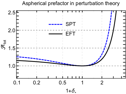
In Fig. 9 we compare the numerical results for $\mathcal{A}_{tot}$ at $z=0$ computed in SPT and upon inclusion of the EFT correction (we use the value $\gamma_{0}=1.5\,(\text{Mpc}/h)^{2}$). We see that the EFT correction has a sizable effect on the prefactor, and somewhat reduces its value.

4.3 Aspherical prefactor at second order in background density

In order to compute the full aspherical prefactor we have to combine the total determinant with the spherical one, see Eq. (C.34). Unlike the total determinant, the spherical determinant differs from unity at leading order in $\delta_{*}$ and yields

$$\begin{split}\mathcal{A}^{\text{LO}}_{\text{ASP}}=\mathcal{D}_{0}^{1/2}=\exp\Bigg{\{}\delta_{*}\left(\frac{4}{21}-\frac{\xi_{r_{*}}}{\sigma^{2}_{r_{*}}}\right)\Bigg{\}}\,.\end{split}$$ (4.27)

Remarkably, the aspherical prefactor at order $O(\delta_{*})$ is fully controlled by translational invariance which forces the corresponding terms in ${\cal A}_{tot}$ to vanish. Thus, the slope of the aspherical prefactor at the origin is encoded in the spherical collapse dynamics. Note that this slope has precisely the value necessary to restore the zero mean of the density contrast, Eqs. (3.14), (3.11). This is an important consistency check of our approach.

Figure 10: Left panel: the aspherical prefactor in perturbation theory at leading (LO) and next-to-leading (NLO) orders shown against the N-body data for cell radius $r_{*}=10$ Mpc$/h$ at $z=0$. Right panel: the corresponding residuals.

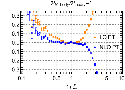
Expanding the monopole determinant, one finds at the next-to-leading order:

$$\begin{split}\mathcal{A}^{\text{NLO}}_{\text{ASP}}=\exp\Bigg{\{}&\delta_{*}\left(\frac{4}{21}-\frac{\xi_{r_{*}}}{\sigma^{2}_{r_{*}}}\right)+\frac{\delta_{*}^{2}}{2}\frac{\sigma^{2}_{\text{1-loop, ren}}}{\sigma^{4}_{r_{*}}}\\ &+\frac{\delta_{*}^{2}}{2}\Bigg{(}-\frac{1180}{1323}+\frac{40\xi_{r_{*}}}{21\sigma^{2}_{r_{*}}}+\frac{r_{*}^{2}\Sigma^{2}_{r_{*}}}{3\sigma^{2}_{r_{*}}}+\frac{\xi_{r_{*}}^{2}}{\sigma^{4}_{r_{*}}}-\frac{3\sigma_{1\,r_{*}}^{2}}{\sigma_{r_{*}}^{2}}\Bigg{)}\Bigg{\}}\,,\end{split}$$ (4.28)

where $\Sigma_{r_{*}}^{2}$ is defined in (4.20) and

$$\sigma^{2}_{1\,r_{*}}=\int_{\bf k}\left(\frac{\sin(kr_{*})}{kr_{*}}\right)^{2}P(k)\,.$$ (4.29)

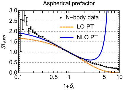
In the left panel of Fig. 10 we show the aspherical prefactor evaluated at leading and next-to-leading orders in perturbation theory. We observe that the LO result works surprisingly well and does not deviate from the data by more than $10\%$ in the range $\delta_{*}\approx[-0.5,1]$, while the NLO results extends the agreement up to $\delta_{*}\approx[-0.8,1.5]$. In the right panel of Fig. 10 we show the residuals for the perturbation theory PDF. One sees that the NLO corrections reduce the residuals close to the origin, but quickly blow up towards large overdensities.

One takes four main lessons from the perturbative calculation:

1. The response matrix contains spurious IR enhanced terms that cancel in the determinant.

2. Including the aspherical corrections amounts, in part, to replacing the linear density variance by its non-linear version.

3. The short-scale contributions should be renormalized by appropriate EFT counterterms.

4. The slope of the aspherical prefactor at the origin is dictated by translational invariance and is such that the mean value $\langle\delta_{*}\rangle$ vanishes.

5 Aspherical prefactor at large density contrasts: main equations

In Sec. 2.3 we expressed the aspherical prefactor as the product of fluctuation determinants in different multipole sectors. Calculation of these determinants requires knowledge of the aspherical response matrices $Q_{\ell}$. In this and the subsequent section we set up the equations for the determination of $Q_{\ell}$ that we will solve numerically afterwards. For simplicity, we work in the EdS approximation. The equations for $\Lambda$CDM cosmology are summarized in Appendix E. We have checked that the difference in the final answers for the prefactor in $\Lambda$CDM and in EdS does not exceed 1%. Thus, the EdS approximation is vastly sufficient for our purposes.

5.1 Linearized fluctuations with $\ell>0$

We first derive the evolution equations for linearized aspherical perturbations in the background of the saddle-point solution. We start from the standard pressureless Euler–Poisson equations for the density, peculiar velocity, and the Newtonian gravitational potential in an EdS universe,

$$\frac{\partial\delta}{\partial t}+\partial_{i}\big{(}(1+\delta)u_{i}\big{)}=0\;,$$ (5.1a)

$$\frac{\partial u_{i}}{\partial t}+{\cal H}u_{i}+(u_{j}\partial_{j})u_{i}=-\partial_{i}\Phi\;,$$ (5.1b)

$$\Delta\Phi=\frac{3{\cal H}^{2}}{2}\delta\;,$$ (5.1c)

where $t$ is conformal time, ${\cal H}=\partial_{t}a/a=2/t$ is the conformal Hubble parameter and $a$ is the scale factor. We expand all quantities into background and first-order perturbations, $\delta=\hat{\delta}+\delta^{(1)}$, etc. Next, we take the divergence of (5.1b) and introduce the velocity potential $\Psi$:

$$u_{i}^{(1)}=-{\cal H}\partial_{i}\Psi^{(1)}~{},~{}~{}~{}~{}\partial_{i}u_{i}^{(1)}=-{\cal H}\Theta^{(1)}\;.$$ (5.2)

From now on we also switch to a new time variable

$$\eta\equiv\mathop{\rm ln}\nolimits a(t)\,,$$ (5.3)

To linear order in perturbations, the system (5.1) takes the form,

$$\dot{\delta}^{(1)}-\Theta^{(1)}+{\cal H}^{-1}\hat{u}_{i}\,\partial_{i}\delta^{(1)}+{\cal H}^{-1}\partial_{i}\hat{u}_{i}\,\delta^{(1)}-\partial_{i}\hat{\delta}\,\partial_{i}\Psi^{(1)}-\hat{\delta}\,\Theta^{(1)}=0\;,$$ (5.4a)

$$\dot{\Theta}^{(1)}+\frac{1}{2}\Theta^{(1)}-\frac{3}{2}\delta^{(1)}+{\cal H}^{-1}\hat{u}_{i}\,\partial_{i}\Theta^{(1)}+{\cal H}^{-1}\partial_{i}\partial_{j}\hat{u}_{j}\,\partial_{i}\Psi^{(1)}+2{\cal H}^{-1}\partial_{i}\hat{u}_{j}\,\partial_{i}\partial_{j}\Psi^{(1)}=0\;,$$ (5.4b)

$$\Delta\Psi^{(1)}=\Theta^{(1)}\;,$$ (5.4c)

where dot denotes the derivative with respect to $\eta$. Note that the background quantities have only radial dependence and the velocity $\hat{u}_{i}$ has only the radial component, so that

$${\cal H}^{-1}\partial_{i}\hat{u}_{j}=-\partial_{i}\partial_{j}\hat{\Psi}=\frac{x_{i}x_{j}}{r^{2}}\partial_{r}^{2}\hat{\Psi}+\bigg{(}\delta_{ij}-\frac{x_{i}x_{j}}{r^{2}}\bigg{)}\frac{\partial_{r}\hat{\Psi}}{r}\;.$$ (5.5)

We now expand the perturbations in spherical harmonics,

$$\delta^{(1)}({\bf x})=\sum_{\ell>0}\sum_{m=-\ell}^{\ell}Y_{\ell m}({\bf x}/r)\,\delta_{\ell m}(r)\;,$$ (5.6)

and similarly for the other fields. To simplify notations, we have omitted the superscript ‘$(1)$’ on the multipole components of the fluctuations. In what follows we will also omit the azimuthal quantum number $m$ as it does not appear explicitly in the equations. Substituting the expansion into Eqs. (5.4) we obtain,

$$\dot{\delta}_{\ell}-\Theta_{\ell}-\partial_{r}\hat{\Psi}\,\partial_{r}\delta_{\ell}-\hat{\Theta}\,\delta_{\ell}-\partial_{r}\hat{\delta}\,\partial_{r}\Psi_{\ell}-\hat{\delta}\,\Theta_{\ell}=0\;,$$ (5.7a)

$$\dot{\Theta}_{\ell}+\frac{1}{2}\Theta_{\ell}-\frac{3}{2}\delta_{\ell}-\partial_{r}\hat{\Psi}\,\partial_{r}\Theta_{\ell}-\partial_{r}\hat{\Theta}\,\partial_{r}\Psi_{\ell}-2\partial_{r}^{2}\hat{\Psi}\,\Theta_{\ell}$$

$$\qquad\qquad\qquad+2\bigg{(}\partial_{r}^{2}\hat{\Psi}-\frac{\partial_{r}\hat{\Psi}}{r}\bigg{)}\,\bigg{(}\frac{2}{r}\partial_{r}\Psi_{\ell}-\frac{\ell(\ell+1)}{r^{2}}\Psi_{\ell}\bigg{)}=0\;,$$ (5.7b)

$$\partial_{r}^{2}\Psi_{\ell}+\frac{2}{r}\partial_{r}\Psi_{\ell}-\frac{\ell(\ell+1)}{r^{2}}\Psi_{\ell}=\Theta_{\ell}\;.$$ (5.7c)

This is a system of (1+1)-dimensional partial differential equations for the set of functions $(\delta_{\ell},\Theta_{\ell},\Psi_{\ell})$.

To determine the initial conditions, we reason as follows. At early times the saddle-point background vanishes and a solution to the previous system goes into

$$\delta_{\ell}(r)\to{\rm e}^{\eta}\,\delta_{L,\ell}(r)\;,$$

where $\delta_{L,\ell}$ is a linear density field. Just like one decomposes linear perturbations over plane waves in 3-dimensional space, we need to choose a basis of functions on the half-line which are properly normalized w.r.t. to the radial integration measure,

$$\int_{0}^{\infty}dr\,r^{2}\,\delta_{L,\ell,k}^{*}(r)\delta_{L,\ell,k^{\prime}}(r)=(2\pi)^{3}k^{-2}\delta_{D}^{(1)}(k-k^{\prime})\;.$$ (5.8)

The expression on the r.h.s. is the radial delta-function compatible with the momentum-space measure $\int[dk]$, Eq. (A.3). A convenient basis with these properties is provided by the spherical Bessel functions (see Appendix A),

$$\delta_{L,\ell,k}(r)=4\pi\,j_{\ell}(kr)\;.$$

We conclude that the relevant initial conditions are,

$$\delta_{\ell,k}(r)=\Theta_{\ell,k}(r)={\rm e}^{\eta}\cdot 4\pi j_{\ell}(kr)\;,$$ (5.9a)

$$\Psi_{\ell,k}=-{\rm e}^{\eta}\cdot\frac{4\pi}{k^{2}}\,j_{\ell}(kr)~{}~{}~{}~{}~{}~{}~{}~{}~{}~{}~{}~{}\text{ at}~{}~{}\eta\to-\infty\;.$$ (5.9b)

In setting up the initial conditions for $\Psi$ we have used that Bessel functions are eigenstates of the radial part of the Laplace operator, see Eq. (A.15).

5.2 Quadratic fluctuations in the monopole sector

To find the response matrix, we need the second-order monopole perturbation $\delta^{(2)}_{0}$ induced by a pair of first-order aspherical modes with a given $\ell$. For simplicity, we will take the latter in the form,

$$\delta^{(1)}_{k}(r)=Y_{\ell,m=0}({\bf x}/r)\,\delta_{\ell,k}(r)\;,$$ (5.10)

so that, according to (A.10), $\delta_{\ell,k}$ is real. Let us first focus on the diagonal elements of the response matrix, i.e. consider the case when the fluctuation $\delta^{(2)}_{0}$ is sourced by two linear modes with the same wavenumber $k$. Generalization to a pair with different wavenumbers will be discussed at the end of the subsection. For compactness we will omit this wavenumber in the subscript of $\delta_{\ell},\Theta_{\ell},\Psi_{\ell}$ in what follows.

Expanding the Euler–Poisson equations to the quadratic order and averaging over the angles we obtain,

$$\dot{\delta}_{0}^{(2)}-\Theta_{0}^{(2)}-\partial_{r}\hat{\Psi}\,\partial_{r}\delta_{0}^{(2)}-\hat{\Theta}\,\delta_{0}^{(2)}-\partial_{r}\hat{\delta}\,\partial_{r}\Psi_{0}^{(2)}-\hat{\delta}\,\Theta_{0}^{(2)}=\Xi_{\delta}\;,$$ (5.11a)

$$\dot{\Theta}_{0}^{(2)}+\frac{1}{2}\Theta_{0}^{(2)}-\frac{3}{2}\delta_{0}^{(2)}-\!\partial_{r}\hat{\Psi}\,\partial_{r}\Theta_{0}^{(2)}-\!\partial_{r}\hat{\Theta}\,\partial_{r}\Psi_{0}^{(2)}$$ (5.11b)

$$~{}~{}~{}~{}~{}~{}~{}~{}~{}~{}~{}~{}~{}~{}~{}~{}~{}~{}-2\partial_{r}^{2}\hat{\Psi}\,\Theta_{0}^{(2)}+\frac{4}{r}\bigg{(}\partial_{r}^{2}\hat{\Psi}-\frac{\partial_{r}\hat{\Psi}}{r}\bigg{)}\,\partial_{r}\Psi_{0}^{(2)}=\Xi_{\Theta}\,,$$

$$\partial_{r}^{2}\Psi_{0}^{(2)}+\frac{2}{r}\partial_{r}\Psi_{0}^{(2)}=\Theta_{0}^{(2)}\;,$$ (5.11c)

where the sources on the r.h.s. are,

$$\Xi_{\delta}=-\frac{1}{\cal H}\int\frac{d\Omega}{4\pi}\,\,\partial_{i}(\delta^{(1)}u_{i}^{(1)})~{},\qquad\Xi_{\Theta}=\frac{1}{{\cal H}^{2}}\int\frac{d\Omega}{4\pi}\,\,\partial_{i}(u_{j}^{(1)}\partial_{j}u_{i}^{(1)})\;.$$ (5.12)

Performing the angular integration and using the Poisson equation (5.7c) the sources can be cast in a suggestive form,

$$\Xi_{\delta}=\frac{1}{r^{2}}\partial_{r}(r^{2}\Upsilon_{\delta})~{},\qquad\Xi_{\Theta}=\frac{1}{r^{2}}\partial_{r}(r^{2}\Upsilon_{\Theta})\;,$$ (5.13)

where

$$\Upsilon_{\delta} =\frac{1}{4\pi}\,\delta_{\ell}\partial_{r}\Psi_{\ell}\;,$$ (5.14a)

$$\Upsilon_{\Theta} =\frac{1}{4\pi}\,\bigg{[}\Theta_{\ell}\partial_{r}\Psi_{\ell}-\frac{2}{r}(\partial_{r}\Psi_{\ell})^{2}+\frac{2\ell(\ell+1)}{r^{2}}\Psi_{\ell}\partial_{r}\Psi_{\ell}-\frac{\ell(\ell+1)}{r^{3}}\Psi_{\ell}^{2}\bigg{]}\;.$$ (5.14b)

Let us introduce a second-order overdensity integrated over a sphere of radius $r_{\eta}$,

$$\mu^{(2)}=\int_{0}^{r_{\eta}}dr\,r^{2}\,\delta_{0}^{(2)}(r)\;,$$ (5.15)

where we allow $r_{\eta}$ to be time dependent. We now show that if $r_{\eta}$ satisfies an appropriate evolution equation, the system (5.11) reduces to an ordinary differential equation for $\mu^{(2)}$. It is convenient to work with the total quantities (background plus second order perturbations), $\delta_{0}=\hat{\delta}+\delta_{0}^{(2)}$ etc. Then Eqs. (5.11) become,

$$\dot{\delta}_{0}-\partial_{r}\Psi_{0}\partial_{r}\delta_{0}-(1+\delta_{0})\Theta_{0}=\Xi_{\delta}\;,$$ (5.16a)

$$\dot{\Theta}_{0}+\frac{1}{2}\Theta_{0}-\frac{3}{2}\delta_{0}-\partial_{r}\Psi_{0}\partial_{r}\Theta_{0}-\Theta_{0}^{2}+\frac{2}{r^{2}}(\partial_{r}\Psi_{0})^{2}+\frac{4}{r}\partial_{r}^{2}\Psi_{0}\partial_{r}\Psi_{0}=\Xi_{\Theta}\;,$$ (5.16b)

$$\partial_{r}(r^{2}\partial_{r}\Psi_{0})=r^{2}\Theta_{0}\;.$$ (5.16c)

Let us multiply the first equation by $r^{2}$ and integrate from $0$ to $r_{\eta}$,

$$\int_{0}^{r_{\eta}}dr\;r^{2}\frac{\partial\delta_{0}}{\partial\eta}-\int_{0}^{r_{\eta}}dr\;r^{2}\partial_{r}\Psi_{0}\partial_{r}\delta_{0}-\int_{0}^{r_{\eta}}dr\;r^{2}(1+\delta_{0})\Theta_{0}=\int_{0}^{r_{\eta}}dr\;r^{2}\Xi_{\delta}\;.$$ (5.17)

The last two terms on the l.h.s. combine into a total derivative due to Eq. (5.16c). Also pulling the time derivative outside of the integral in the first term we obtain,

$$\frac{d}{d\eta}\int_{0}^{r_{\eta}}dr\;r^{2}\big{(}1+\delta_{0}(r)\big{)}-r_{\eta}^{2}\big{(}1+\delta_{0}(r_{\eta})\big{)}\big{(}\dot{r}_{\eta}+\partial_{r}\Psi_{0}(r_{\eta})\big{)}=r^{2}_{\eta}\Upsilon_{\delta}(r_{\eta})\;.$$ (5.18)

The boundary terms on the l.h.s. cancel if we choose the time-dependence of $r_{\eta}$ in such a way that

$$\dot{r}_{\eta}=-\partial_{r}\Psi_{0}(r_{\eta})\;.$$ (5.19)

In other words, we shall choose the boundary to be moving with the angular-averaged fluid velocity. Then Eq. (5.18) simplifies,

$$\dot{\mu}=r^{2}_{\eta}\Upsilon_{\delta}(r_{\eta})\;,$$ (5.20)

where we introduced

$$\mu=\int_{0}^{r_{\eta}}dr\;r^{2}\big{(}1+\delta_{0}(r)\big{)}.$$ (5.21)

This equation has a clear physical interpretation. It tells us that the mass inside a spherical region comoving with the average spherical fluid flow changes due to the inflow through the boundary generated by aspherical modes.

Equation (5.20) allows us to determine $\mu$ once the time dependence of $r_{\eta}$ is known. However, we still need an evolution equation for $r_{\eta}$ in terms of $r_{\eta}$ and $\mu$ to close the system. This is obtained from (5.16b) by multiplying it with $r^{2}$ and integrating from $0$ to $r_{\eta}$. Using (5.13) and (5.14b) we obtain,

$$r_{\eta}^{2}\bigg{(}\frac{\partial}{\partial\eta}\partial_{r}\Psi_{0}+\frac{1}{2}\partial_{r}\Psi_{0}-\partial_{r}\Psi_{0}\partial_{r}^{2}\Psi_{0}\bigg{)}\bigg{|}_{r_{\eta}}-\frac{3}{2}\bigg{(}\mu-\frac{r^{3}_{\eta}}{3}\bigg{)}=r_{\eta}^{2}\Upsilon_{\Theta}(r_{\eta})\;.$$ (5.22)

It follows from (5.19) that

$$\ddot{r}_{\eta}=\bigg{(}-\frac{\partial}{\partial\eta}\partial_{r}\Psi_{0}+\partial^{2}_{r}\Psi_{0}\partial_{r}\Psi_{0}\bigg{)}\bigg{|}_{r_{\eta}}\;.$$ (5.23)

Thus, we arrive at

$$\ddot{r}_{\eta}+\frac{\dot{r}_{\eta}}{2}-\frac{r_{\eta}}{2}+\frac{3\mu}{2r_{\eta}^{2}}=-\Upsilon_{\Theta}(r_{\eta})\;.$$ (5.24)

There is again a transparent physical interpretation: the aspherical perturbations exert an effective force on the spherical flow that modifies its acceleration.

As a final step, we decompose $\mu$ and $r_{\eta}$ into background values and second-order perturbations,

$$r_{\eta}=\hat{r}_{\eta}+r^{(2)}_{\eta}\;,$$ (5.25a)

$$\mu=\hat{\mu}+\mu^{(2)}+r_{\eta}^{(2)}\hat{r}_{\eta}^{2}\big{(}1+\hat{\delta}(\hat{r}_{\eta})\big{)}\;,$$ (5.25b)

where $\hat{r}_{\eta}$, $\hat{\mu}$ satisfy source-free Eqs. (5.20), (5.24). Subtracting the background contributions from the evolution equations we obtain,

$$\dot{\mu}^{(2)}+\dot{r}_{\eta}^{(2)}\hat{r}_{\eta}^{2}\big{(}1+\hat{\delta}(\hat{r}_{\eta})\big{)}+r_{\eta}^{(2)}\frac{d}{d\eta}\Big{(}\hat{r}_{\eta}^{2}\big{(}1+\hat{\delta}(\hat{r}_{\eta})\big{)}\Big{)}=\hat{r}_{\eta}^{2}\Upsilon_{\delta}(\hat{r}_{\eta})\;$$ (5.26a)

$$\ddot{r}^{(2)}_{\eta}+\frac{\dot{r}_{\eta}^{(2)}}{2}+\bigg{(}1+\frac{3}{2}\hat{\delta}(\hat{r}_{\eta})-\frac{R_{*}^{3}}{\hat{r}_{\eta}^{3}}\bigg{)}r^{(2)}_{\eta}+\frac{3}{2\hat{r}_{\eta}^{2}}\mu^{(2)}=-\Upsilon_{\Theta}(\hat{r}_{\eta})\;,$$ (5.26b)

where we have used the asymptotics $\hat{r}_{\eta}\to R_{*}$, $\hat{\mu}\to R^{3}_{*}/3$ at $\eta\to-\infty$. Equations (5.26) provide a closed system of linear ordinary differential equations for the variables $\mu_{*}^{(2)}$, $r^{(2)}_{\eta}$ once the sources $\Upsilon_{\delta,\Theta}$ are known.

We must supplement (5.26) by three boundary conditions. One of them is set at the final time and expresses the fact that we are interested in the overdensity within the fixed radius $r_{*}$, so that the final radius is not perturbed,

$$r^{(2)}_{\eta}\big{|}_{\eta=0}=0\;.$$ (5.27a)

The conditions at the initial time $$\eta\to-\infty \delta_{0} {\rm e}^{\eta} {\rm e}^{2\eta}$$ are more subtle. The source-free Eqs. (5.26) admit solutions corresponding to first order monopole fluctuations, that can also change the mass within the cell. We need to eliminate such solutions. For this purpose, we observe that for the spurious solutions the fields etc. behave as at early times, whereas the second-order perturbations that we are interested in are proportional to . We conclude that we must require,

$$\mu^{(2)}\propto{\rm e}^{2\eta}~{},\quad\text{at}~{}\eta\to-\infty\;.$$ (5.27b)

As for $$r_{\eta}^{(2)} \dot{\hat{\mu}} r_{\eta}^{(2)}\hat{r}_{\eta}^{2}\big{(}1+\hat{\delta}(\hat{r}_{\eta})\big{)} {\rm e}^{2\eta}$$, it need not vanish in the beginning. Rather, it should approach a constant value in a specific way. Indeed, from Eqs. (5.20), (5.25b) and the fact that vanishes we conclude that the derivative of the combination must fall off as . Thus, we obtain the third condition,

$$\dot{r}_{\eta}^{(2)}+r_{\eta}^{(2)}\frac{d}{d\eta}\mathop{\rm ln}\nolimits\big{[}\hat{r}^{2}_{\eta}\big{(}1+\hat{\delta}(\hat{r}_{\eta})\big{)}\big{]}\propto{\rm e}^{2\eta}~{},\quad\text{at}~{}\eta\to-\infty\;.$$ (5.27c)

It is straightforward to generalize the above analysis to the case when the second-order perturbation is sourced by a pair of aspherical modes with different radial wavenumbers $k$ and $k^{\prime}$ (but, of course, the same angular numbers $\ell$ and $m$). In that case the sources (5.14) are replaced by symmetric combinations constructed from the two modes,

$$\Upsilon_{\delta,kk^{\prime}} =\frac{1}{8\pi}\,\delta_{\ell,k}\partial_{r}\Psi_{\ell,k^{\prime}}+(k\longleftrightarrow k^{\prime})\;,$$ (5.28a)

$$\Upsilon_{\Theta,kk^{\prime}} =\frac{1}{8\pi}\,\bigg{[}\Theta_{\ell,k}\partial_{r}\Psi_{\ell,k^{\prime}}-\frac{2}{r}\partial_{r}\Psi_{\ell,k}\partial_{r}\Psi_{\ell,k^{\prime}}+\frac{2\ell(\ell+1)}{r^{2}}\Psi_{\ell,k}\partial_{r}\Psi_{\ell,k^{\prime}}$$

$$~{}~{}~{}~{}~{}~{}~{}~{}~{}~{}-\frac{\ell(\ell+1)}{r^{3}}\Psi_{\ell,k}\Psi_{\ell,k^{\prime}}\bigg{]}+(k\longleftrightarrow k^{\prime})\;.$$ (5.28b)

The rest of the derivation goes exactly the same as above, leading to Eqs. (5.26) with the new sources.

5.3 Summary of the algorithm

Summarizing the results of this section, one obtains the following algorithm to find the response matrix $Q_{\ell}(k,k^{\prime})$ and the fluctuation determinant ${\cal D}_{\ell}$:

1. One solves Eqs. (5.7) with the initial conditions (5.9) and finds the mode functions $\delta_{\ell},\Theta_{\ell},\Psi_{\ell}$ for each basis function from a set of $N+1$ momenta $\{k_{0},...,k_{N}\}$.

2. One uses these solutions to construct the sources (5.28) for a pair of wavevectors $k_{i}$ and $k_{j}$.

3. One solves (5.26) with the initial conditions (5.27) . The final variation in the averaged overdensity gives the element of $Q_{\ell}$,

   $$Q_{\ell}(k_{i},k_{j})=\frac{3}{r_{*}^{3}}\mu^{(2)}(\eta=0)\;.$$ (5.29)

4. One repeats the above procedure for all different pairs of wavenumbers $(k_{i},k_{j})$, construct the operator $\mathbb{1}+2\hat{\lambda}\sqrt{P}Q_{\ell}\sqrt{P}$ and evaluates its determinant.

The implementation of this algorithm on a discrete grid is described in Appendix G.

The algorithm requires a modification in the dipole sector ($\ell=1$) due to the IR sensitivity of the matrix $Q_{1}$. We now focus on this issue.

6 Removing IR divergences in the dipole contribution

A complication arises in the dipole sector ($\ell=1$). The initial conditions (5.9b) imply that the velocity potential $\Psi_{1,k}\propto{\rm e}^{\eta}\cdot r/k$ has an $1/k$ pole at $kr\sim kr_{*}\ll 1$. Substitution of this expressions into equations of motion (5.7a), (5.7) leads to further $1/k$ contributions in $\delta_{1,k}$ and $\Theta_{1,k}$ proportional to the derivatives of the background configuration $\partial_{r}\hat{\delta}$, $\partial_{r}\hat{\Theta}$. Thus, the linear solution $(\delta_{1},\Theta_{1},\Psi_{1})$ contains singular $1/k$ terms which translate into first- and second-order poles in the matrix $Q_{1}(k,k^{\prime})$ at $k,k^{\prime}\ll 1/r_{*}$. As we discuss below, these infrared (IR) enhanced contribution must cancel in the determinant ${\cal D}_{1}$ entering the prefactor (2.44), which is IR-safe. However, the presence of the ‘IR-divergent’ terms makes a straightforward numerical evaluation of the determinant unfeasible. The purpose of this section is to show that the IR-enhanced contributions can be isolated and the IR-divergences can be removed, whereby reducing the task to numerical evaluation of IR-safe quantities only.

6.1 IR safety of the prefactor

We start by showing that the aspherical prefactor (2.44) is IR safe. We first give a heuristic argument and then a more direct proof. Let us assume that the mapping from the linear to non-linear density fields is invertible. Then the counts-in-cells PDF can be written in the schematic form,

$${\cal P}(\delta_{*})={\cal N}^{-1}\int\mathscr{D}\delta\,\int\frac{d\lambda}{2\pi ig^{2}}\,\exp\left\{-\frac{\Gamma[\delta]}{g^{2}}+\frac{\lambda}{g^{2}}\left(\delta_{*}-\bar{\delta}(r_{*})\right)\right\}\;,$$ (6.1)

where the path integral runs over all density configurations at the final moment of time and $\Gamma[\delta]$ is a weighting functional obtained from the Gaussian weight using the map $\delta\mapsto\delta_{L}$. A perturbative expansion for the functional $\Gamma[\delta]$ was derived in [9] and it was shown that all coefficients in this expansion are IR-safe. Extrapolating this property to the non-perturbative level, one concludes that the matrix of second variational derivatives around the saddle-point solution

$$\frac{\partial^{2}\Gamma}{\partial\delta^{(1)}({\bf x})\,\partial\delta^{(1)}({\bf x}^{\prime})}\bigg{|}_{\delta=\hat{\delta}({\bf x})}\;$$ (6.2)

is also IR-safe. The prefactor of the PDF is given by the determinant of this matrix, hence it is IR-safe as well.

We now give a more rigorous argument that does not require invertibility of the density mapping. We split the integration variables in the path integral (2.7) into soft ($k\ll 1/r_{*}$) and hard ($k\gtrsim 1/r_{*}$) modes. Omitting for clarity the normalization factors we obtain,

$${\cal P}(\delta_{*})=\int\mathscr{D}\delta^{\rm soft}_{L}\exp\bigg{\{}-\int_{\bf k}\frac{|\delta_{L}^{\rm soft}({\bf k})|^{2}}{2g^{2}P(k)}\bigg{\}}\;{\cal P}[\delta_{*};\delta_{L}^{\rm soft}]\;,$$ (6.3)

where

$${\cal P}[\delta_{*};\delta_{L}^{\rm soft}]\equiv\int\mathscr{D}\delta_{L}^{\rm hard}\,d\lambda\,\exp\left\{-\frac{1}{g^{2}}\bigg{[}\int_{\bf k}\frac{|\delta_{L}^{\rm hard}({\bf k})|^{2}}{2P(k)}-\lambda\big{(}\delta_{*}-\bar{\delta}_{W}[\delta_{L}^{\rm hard}+\delta_{L}^{\rm soft}]\big{)}\bigg{]}\right\}\;,$$ (6.4)

has the physical meaning of the PDF for short-scale overdensities in the background of soft modes.

Now, the addition of a soft mode corresponds to immersion of the system into a large-scale flow. Due to the equivalence principle, the main effect of such flow is an overall translation of the hard modes by a distance proportional to the gradient of the Newtonian potential [4, 5, 6, 7, 8]. In other words,

$$\delta[\delta_{L}^{\rm hard}+\delta_{L}^{\rm soft}]({\bf x},\eta)=\delta[\delta_{L}^{\rm hard}]\Big{(}{\bf x}-\frac{\nabla}{\Delta}\delta_{L}^{\rm soft}(0,\eta),\eta\Big{)}+\ldots\;.$$ (6.5)

The shift is enhanced for long-wavelength perturbations leading to $1/k_{\rm soft}$ poles in the perturbative expansion of the expression (6.5) in $\delta_{L}^{\rm soft}$. On the other hand, the remaining terms represented by dots in (6.5) contain more derivatives acting on the Newtonian potential, and thus are regular in the limit when the soft momentum $k_{\rm soft}$ goes to zero.

The PDF (6.4) can be evaluated in the saddle-point approximation. The saddle-point solution is

$$\hat{\delta}_{L}[\delta_{L}^{\rm soft}]({\bf x})=\hat{\delta}_{L}\Big{(}{\bf x}+\frac{\nabla}{\Delta}\delta_{L}^{\rm soft}|_{{\bf x}=0}\Big{)}\;,$$ (6.6)

where $\hat{\delta}_{L}$ is the saddle-point configuration in the absence of soft modes. Likewise, the fluctuations around the solution (6.6) are obtained from those around $\hat{\delta}_{L}$ by the same translation, so that the integral over them does not contain any poles. We conclude that ${\cal P}[\delta_{*};\delta_{L}^{\rm soft}]$ is IR-safe which implies the IR safety of the original PDF ${\cal P}(\delta_{*})$.

6.2 Factorization of IR divergences

At $\ell=1$ the equations (5.7) admit an exact solution

$$\delta_{1}=\partial_{r}\hat{\delta}\cdot{\rm e}^{\eta}~{},~{}~{}~{}~{}\Theta_{1}=\partial_{r}\hat{\Theta}\cdot{\rm e}^{\eta}~{},~{}~{}~{}~{}\Psi_{1}=\partial_{r}\hat{\Psi}\cdot{\rm e}^{\eta}+r\cdot{\rm e}^{\eta}\;.$$ (6.7)

Notice that in the far past all contributions here vanish faster than ${\rm e}^{\eta}$ (actually, as $O({\rm e}^{2\eta})$), except for the last term in $\Psi_{1}$. The latter corresponds to a uniform motion of all fluid elements, i.e. to a large bulk flow. Existence of the solution (6.7) follows from the equivalence principle obeyed by the Euler-Poisson equations. Indeed, we can impose on any solution an infinitely large bulk flow that will sweep the original solution as a whole. The dipolar solution (6.7) precisely corresponds to imposing such a large bulk flow on the saddle-point configuration $(\hat{\delta},\hat{\Theta},\hat{\Psi})$.

The solution (6.7) can be added with an arbitrary coefficient to any other solution of eqs. (5.7). In particular, the perturbation with the initial conditions (5.9) for $\ell=1$ can be written as,

$$\delta_{1,k}=\breve{\delta}_{k}-\frac{4\pi}{3k}\partial_{r}\hat{\delta}\,{\rm e}^{\eta}\;,$$ (6.8a)

$$\Theta_{1,k}=\breve{\Theta}_{k}-\frac{4\pi}{3k}\partial_{r}\hat{\Theta}\,{\rm e}^{\eta}\;,$$ (6.8b)

$$\Psi_{1,k}=\breve{\Psi}_{k}-\frac{4\pi}{3k}\partial_{r}\hat{\Psi}\,{\rm e}^{\eta}-\frac{4\pi r}{3k}\,{\rm e}^{\eta}\;,$$ (6.8c)

where the triple $\big{(}\breve{\delta}_{k},\breve{\Theta}_{k},\breve{\Psi}_{k}\big{)}$ is also a solution of eqs. (5.7) satisfying the same initial conditions (5.9a) for $\breve{\delta}_{k}$, $\breve{\Theta}_{k}$, but with modified initial condition for $\breve{\Psi}_{k}$,

$$\breve{\Psi}_{k}=\bigg{[}-\frac{4\pi}{k^{2}}j_{1}(kr)+\frac{4\pi r}{3k}\bigg{]}\cdot{\rm e}^{\eta}\;.$$ (6.9)

Importantly, this modification eliminates the dangerous $1/k$ pole, so that the initial conditions for all functions $(\breve{\delta}_{k},\breve{\Theta}_{k},\breve{\Psi}_{k})$ are regular at $k\to 0$. In fact,

$$\breve{\delta}_{k},\breve{\Theta}_{k},\breve{\Psi}_{k}=O(k)\;.$$ (6.10)

Then, by linearity of eqs. (5.7), this property holds at all times.

The next step is to isolate the IR divergences in the sources $\Upsilon_{\delta}$, $\Upsilon_{\Theta}$. Substituting (6.8) into (5.28), we obtain

$$\Upsilon_{\delta,kk^{\prime}}=\frac{A_{\delta}}{kk^{\prime}}+\frac{B_{\delta,k^{\prime}}}{k}+\frac{B_{\delta,k}}{k^{\prime}}+\breve{\Upsilon}_{\delta,kk^{\prime}}\;,$$ (6.11a)

$$\Upsilon_{\Theta,kk^{\prime}}=\frac{A_{\Theta}}{kk^{\prime}}+\frac{B_{\Theta,k^{\prime}}}{k}+\frac{B_{\Theta,k}}{k^{\prime}}+\breve{\Upsilon}_{\Theta,kk^{\prime}}\;,$$ (6.11b)

where

$$A_{\delta}=\frac{4\pi}{9}\partial_{r}\hat{\delta}(\partial^{2}_{r}\hat{\Psi}+1)\,{\rm e}^{2\eta}\;,$$ (6.12a)

$$B_{\delta,k}=-\frac{1}{6}\big{[}(\partial_{r}^{2}\hat{\Psi}+1)\breve{\delta}_{k}+\partial_{r}\hat{\delta}\partial_{r}\breve{\Psi}_{k}\big{]}\,{\rm e}^{\eta}\;,$$ (6.12b)

$$A_{\Theta}=\frac{4\pi}{9}\bigg{[}\partial_{r}\hat{\Theta}(\partial^{2}_{r}\hat{\Psi}+1)-\frac{2}{r}(\partial_{r}^{2}\hat{\Psi})^{2}+\frac{4}{r^{2}}\partial_{r}\hat{\Psi}\partial_{r}^{2}\hat{\Psi}-\frac{2}{r^{3}}(\partial_{r}\hat{\Psi})^{2}\bigg{]}\,{\rm e}^{2\eta}\;,$$ (6.12c)

$$B_{\Theta,k}\!=\!-\frac{1}{6}\bigg{[}(\partial_{r}^{2}\hat{\Psi}\!+\!1)\breve{\Theta}_{k}\!+\!\bigg{(}\!\partial_{r}\hat{\Theta}\!-\!\frac{4}{r}\partial_{r}^{2}\hat{\Psi}\!+\!\frac{4}{r^{2}}\partial_{r}\hat{\Psi}\!\bigg{)}\partial_{r}\breve{\Psi}_{k}\!+\!\bigg{(}\frac{4}{r^{2}}\partial_{r}^{2}\hat{\Psi}\!-\!\frac{4}{r^{3}}\partial_{r}\hat{\Psi}\!\bigg{)}\breve{\Psi}_{k}\bigg{]}\,{\rm e}^{\eta}\,,$$ (6.12d)

and $\breve{\Upsilon}_{\delta,kk^{\prime}}$, $\breve{\Upsilon}_{\Theta,kk^{\prime}}$ are computed using the regular solutions $(\breve{\delta}_{k},\breve{\Theta}_{k},\breve{\Psi}_{k})$, $(\breve{\delta}_{k^{\prime}},\breve{\Theta}_{k^{\prime}},\breve{\Psi}_{k^{\prime}})$. Due to linearity of Eqs. (5.26), the pole structure of the sources (6.11) propagates into the pole structure of the matrix

$$Q_{1}(k,k^{\prime})=\frac{A}{kk^{\prime}}+\frac{B(k^{\prime})}{k}+\frac{B(k)}{k^{\prime}}+\breve{Q}(k,k^{\prime})\;,$$ (6.13)

where $A$, $B$, $\breve{Q}$ are found by solving Eqs. (5.26) with the sources $(A_{\delta},A_{\Theta})$, $(B_{\delta},B_{\Theta})$ and $(\breve{\Upsilon}_{\delta},\breve{\Upsilon}_{\Theta})$ respectively. Due to the property (6.10) we have

$$B(k)=O(k)~{},~{}~{}~{}~{}\breve{Q}(k,k^{\prime})=O(kk^{\prime})~{}~{}~{}\text{at}~{}k,k^{\prime}\to 0\;.$$ (6.14)

We now observe that the sought-for determinant has the form,

$$\mathcal{D}_{1}=\det\Big{(}\mathbb{1}+2\hat{\lambda}\sqrt{P}\breve{Q}\sqrt{P}+a(k)b(k^{\prime})+b(k)a(k^{\prime})\Big{)}\;,$$ (6.15)

with

$$a(k)=\hat{\lambda}\frac{\sqrt{P(k)}}{k}~{},~{}~{}~{}~{}~{}b(k)=\bigg{(}\frac{A}{k}+2B(k)\bigg{)}\sqrt{P(k)}\;.$$ (6.16)

Denoting

$$M(k,k^{\prime})=(2\pi)^{3}k^{-2}\delta_{\rm D}^{(1)}(k-k^{\prime})+2\hat{\lambda}\sqrt{P(k)}\breve{Q}(k,k^{\prime})\sqrt{P(k^{\prime})}$$ (6.17)

we write,

$$\mathcal{D}_{1}=\det M\cdot\mathcal{D}^{IR}\;,$$ (6.18)

where all IR-sensitive contributions have been collected into

$$\mathcal{D}^{IR}=\det\big{(}\mathbb{1}+\tilde{a}\otimes\tilde{b}+\tilde{b}\otimes\tilde{a}\big{)}\;.$$ (6.19)

We have introduced $\tilde{a}=M^{-1/2}a$, $\tilde{b}=M^{-1/2}b$ and used the fact that the matrix $M$ is symmetric.

The determinant (6.19) can be easily evaluated using Eq. (D.1) from Appendix D,

$$\mathcal{D}^{IR}=1+2(\tilde{a}\cdot\tilde{b})+(\tilde{a}\cdot\tilde{b})^{2}-\tilde{a}^{2}\,\tilde{b}^{2}\;.$$ (6.20)

Here dot denotes the scalar product,

$$\tilde{a}\cdot\tilde{b}=\int[dk]\,\tilde{a}(k)\tilde{b}(k)=\int[dk][dk^{\prime}]\,a(k)M^{-1}(k,k^{\prime})b(k^{\prime})\;,$$

and similarly for $\tilde{a}^{2}$ and $\tilde{b}^{2}$. The inverse matrix $M^{-1}$ has the form,

$$M^{-1}=\mathbb{1}-2\hat{\lambda}\sqrt{P}\mathring{Q}\sqrt{P}$$ (6.21)

with

$$\mathring{Q}(k,k^{\prime})=\breve{Q}(k,k^{\prime})+\ldots=O(kk^{\prime})~{}~{}~{}\text{at small}~{}k,k^{\prime}\;.$$ (6.22)

Using this property one isolates the ‘IR-divergences’ in the different terms in (6.20),

$$2(\tilde{a}\cdot\tilde{b}) \ni 2\hat{\lambda}\int[dk]\frac{P(k)}{k^{2}}A$$ (6.23a)

$$(\tilde{a}\cdot\tilde{b})^{2} -\tilde{a}^{2}\tilde{b}^{2}\ni-4\hat{\lambda}^{2}\int[dk]^{2}\frac{P(k_{1})}{k_{1}^{2}}P(k_{2})\big{(}B(k_{2})\big{)}^{2}$$

$$\qquad\qquad\;+8\hat{\lambda}^{3}\int[dk]^{3}\frac{P(k_{1})}{k_{1}^{2}}P(k_{2})P(k_{3})\mathring{Q}(k_{2},k_{3})B(k_{2})B(k_{3})\;.$$ (6.23b)

A necessary and sufficient condition for their cancellation in the determinant (6.20) is,

$$A=2\hat{\lambda}\int[dk]^{2}\sqrt{P(k_{1})P(k_{2})}B(k_{1})M^{-1}(k_{1},k_{2})B(k_{2})\;.$$ (6.24)

While we do not have a direct proof of this identity, the arguments of the previous subsection imply that it must be satisfied. We also checked it numerically and found that it is fulfilled in our computations within the accuracy of the numerical procedure.

Using (6.24) we can simplify the expression (6.20). A straightforward calculation yields,

$$\mathcal{D}^{IR}=\bigg{[}1+2\hat{\lambda}\int[dk]^{2}\sqrt{P(k_{1})P(k_{2})}\;\frac{1}{k_{1}}M^{-1}(k_{1},k_{2})B(k_{2})\bigg{]}^{2}\;.$$ (6.25)

This is the final expression to be used in numerical evaluation. The algorithm for the computation of ${\cal D}_{1}$ consists of the following steps:

1. Solve the linear equations (5.7) with initial conditions (5.9a), (6.9) to find the functions $\breve{\delta}_{k}$, $\breve{\Theta}_{k}$, $\breve{\Psi}_{k}$;

2. Find the matrix $\breve{Q}(k,k^{\prime})$ by solving Eqs. (5.26) with the sources $\breve{\Upsilon}_{\delta,kk^{\prime}}$, $\breve{\Upsilon}_{\Theta,kk^{\prime}}$;

3. Find the vector $B(k)$ by solving Eqs. (5.26) with the sources $B_{\delta,k}$, $B_{\Theta,k}$,
   Eqs. (6.12b), (6.12d);

4. Construct the matrix $M(k,k^{\prime})$, Eq. (6.17), compute its determinant and inverse;

5. Use the inverse matrix $M^{-1}(k,k^{\prime})$ and the vector $B(k)$ to compute the IR contribution (6.25);

6. Compute the full determinant in the dipole sector as a product of $\det M$ and $\mathcal{D}^{IR}$.

7 WKB approximation for high multipoles

In general the computation of the aspherical fluctuation determinant requires solving the system of linear partial differential equations (5.7) on a grid. However, in the sectors with large orbital numbers $\ell\gg 1$ one can use the Wentzel-Kramers-Brillouin (WKB) technique to simplify the problem and gain insights into the structure of the aspherical response matrix. Remarkably, in the WKB regime the system (5.7) reduces to a system of ordinary differential equations and can be easily solved, e.g. in Mathematica. The WKB analysis serves both to cross check the results of the full numerical integration of Eqs. (5.7) and to study the UV sensitivity of the aspherical prefactor in Sec. 8.2.

We start by noticing that the basis functions (5.9) are suppressed at $kr<\ell$ due to the centrifugal barrier. Indeed, at these values of $r$ we obtain using Eq. (10.19.3) from [60],

$$j_{\ell}\big{(}(\ell+1/2)\varkappa r\big{)}\sim\frac{e^{-(\ell+1/2)\big{(}{\rm arcch}\frac{1}{\varkappa r}-\sqrt{1-(\varkappa r)^{2}}\big{)}}}{(2\ell+1)\sqrt{\varkappa r}[1-(\varkappa r)^{2}]^{1/4}}\;,$$ (7.1)

where we have introduced the ratio

$$\varkappa\equiv\frac{k}{\ell+1/2}$$ (7.2)

which will be kept fixed in the limit $\ell\to\infty$. We see that $j_{\ell}(kr)$ is exponentially suppressed at $\varkappa r<1$. Thus, if $kr_{*}\ll\ell$ the perturbation has support outside of the window function and does not contribute into the variation of the overdensity: $Q_{\ell}(k,k^{\prime})\approx 0$ whenever $k$ or $k^{\prime}$ is much smaller than $\ell/r_{*}$. We conclude that the dominant contribution into the response matrix comes from the modes with

$$k\gtrsim\ell/r_{*}\gg 1/r_{*}\;.$$ (7.3)

These modes oscillate much faster than the background, so we can use the WKB technique to find their evolution.

We will see that we have to go up to the second order in the WKB expansion, hence we write the following Ansatz:

$$\begin{split}&\delta_{\ell}=(\delta_{\ell 1}+k^{-1}\delta_{\ell 2}){\rm e}^{ikS_{\ell}}+{\rm h.c.}~{},~{}~{}\\ &\Theta_{\ell}=(\Theta_{\ell 1}+k^{-1}\Theta_{\ell 2}){\rm e}^{ikS_{\ell}}+{\rm h.c.}~{},~{}~{}\\ &\Psi_{\ell}=\!(k^{-2}\Psi_{\ell 1}+k^{-3}\Psi_{\ell 2}){\rm e}^{ikS_{\ell}}+{\rm h.c.}\end{split}$$ (7.4)

where $\delta_{\ell 1},\delta_{\ell 2}$ etc. are slowly varying functions. Note that $\Psi_{\ell}$ is suppressed by two powers of $k$ compared to $\delta_{\ell}$ and $\Theta_{\ell}$. From the Poisson equation (5.7c) we find at leading order

$$\Psi_{\ell 1}=-\frac{\Theta_{\ell 1}}{(S_{\ell}^{\prime})^{2}+(\varkappa r)^{-2}}\;.$$ (7.5a)

The next-to-leading expansion yields,

$$\Psi_{\ell 2}=\frac{-\Theta_{\ell 2}+iS_{\ell}^{\prime\prime}\Psi_{\ell 1}+2iS_{\ell}^{\prime}\Psi_{\ell 1}^{\prime}+\frac{2iS_{\ell}^{\prime}}{r}\Psi_{\ell 1}}{(S_{\ell}^{\prime})^{2}+(\varkappa r)^{-2}}\;.$$ (7.5b)

Further, we susbstitute the form (7.4) into the dynamical Eqs. (5.7a), (5.7). At leading order $O(k)$ both equations reduce to

$$\dot{S}_{\ell}-\partial_{r}\hat{\Psi}S_{\ell}^{\prime}=0\;.$$ (7.6)

In the combination on the l.h.s. one recognizes the time-derivative along the background flow, so one concludes that $S_{\ell}$ is conserved along the flow,

$$\frac{dS_{\ell}}{d\eta}\bigg{|}_{\rm flow}=0\;.$$ (7.7)

In other words, $S_{\ell}(r,\eta)=S_{\ell}\big{(}R(r,\eta)\big{)}$, where $R$ is the Lagrangian coordinate of the spherical shell in the background solution. It is related to the Eulerian coordinate $r$ and $\eta$ by Eq. (2.13) where for the density contrast one takes the saddle-point profile $\hat{\delta}(r,\eta)$. At $\eta\to-\infty$ the Lagrangian and Eulerian coordinates coincide, $R=r$.

From the orders $O(1)$ and $O(1/k)$ of Eqs. (5.7a), (5.7) we obtain the equations for the coefficient functions in the WKB Ansatz:
Next-to Leading Order,

$$\frac{d\delta_{\ell 1}}{d\eta}\bigg{|}_{\rm flow}-\hat{\Theta}\delta_{\ell 1}-(1+\hat{\delta})\Theta_{\ell 1}=0\;,$$ (7.8a)

$$\frac{d\Theta_{\ell 1}}{d\eta}\bigg{|}_{\rm flow}-\frac{3}{2}\delta_{\ell 1}+\bigg{[}\frac{1}{2}-\frac{2(\varkappa rS_{\ell}^{\prime})^{2}\partial_{r}^{2}\hat{\Psi}}{1+(\varkappa rS_{\ell}^{\prime})^{2}}-\frac{2\partial_{r}\hat{\Psi}}{r(1+(\varkappa rS_{\ell}^{\prime})^{2})}\bigg{]}\Theta_{\ell 1}=0\;.$$ (7.8b)

Next-to-Next-to-Leading Order,

$$\frac{d\delta_{\ell 2}}{d\eta}\bigg{|}_{\rm flow}- \hat{\Theta}\delta_{\ell 2}-(1+\hat{\delta})\Theta_{\ell 2}=i\partial_{r}\hat{\delta}\,S_{\ell}^{\prime}\Psi_{\ell 1}\;,$$ (7.9a)

$$\frac{d\Theta_{\ell 2}}{d\eta}\bigg{|}_{\rm flow}- \frac{3}{2}\delta_{\ell 2}+\bigg{[}\frac{1}{2}-\frac{2(\varkappa rS_{\ell}^{\prime})^{2}\partial_{r}^{2}\hat{\Psi}}{1+(\varkappa rS_{\ell}^{\prime})^{2}}-\frac{2\partial_{r}\hat{\Psi}}{r(1+(\varkappa rS_{\ell}^{\prime})^{2})}\bigg{]}\Theta_{\ell 2}$$

$$= \frac{4iS_{\ell}^{\prime}}{1+(\varkappa rS_{\ell}^{\prime})^{2}}\bigg{(}\partial_{r}^{2}\hat{\Psi}-\frac{\partial_{r}\hat{\Psi}}{r}\bigg{)}\Psi_{\ell 1}^{\prime}$$

$$+\bigg{[}i\partial_{r}\hat{\Theta}S_{\ell}^{\prime}+\frac{2i}{1+(\varkappa rS_{\ell}^{\prime})^{2}}\bigg{(}S_{\ell}^{\prime\prime}-\frac{2S_{\ell}^{\prime}(\varkappa rS_{\ell}^{\prime})^{2}}{r}\bigg{)}\bigg{(}\partial_{r}^{2}\hat{\Psi}-\frac{\partial_{r}\hat{\Psi}}{r}\bigg{)}\bigg{]}\Psi_{\ell 1}\;.$$ (7.9b)

We notice that Eqs. (7.8) do not contain spatial derivatives of $\delta_{\ell 1},\Theta_{\ell 1}$, so that they form a system of ordinary differential equations for these functions. The same is true for Eqs. (7.9) with respect to the functions $\delta_{\ell 2},\Theta_{\ell 2}$.

To set up the initial conditions we use the asymptotic expansion for the Bessel function at large order (Eq. (10.19.6) from [60]),

$$j_{\ell}\bigg{(}\!\frac{\ell\!+\!1/2}{\cos\beta}\!\bigg{)}=\frac{\cos\beta}{(\ell\!+\!1/2)\sqrt{\sin\beta}}\bigg{(}\!\!\cos\xi+\frac{1}{8(\ell\!+\!1/2)}\bigg{(}\!\mathop{\rm ctg}\nolimits\beta+\frac{5}{3}(\mathop{\rm ctg}\nolimits\beta)^{3}\bigg{)}\sin\xi+O(\ell^{-2})\!\bigg{)}\;,$$ (7.10)

where

$$\xi=(\ell+1/2)(\mathop{\rm tg}\nolimits\beta-\beta)-\pi/4\;.$$ (7.11)

Substituting this into (5.9) and comparing with the WKB Ansatz (7.4) we find the initial conditions at $\eta\to-\infty$,

$$S_{\ell}=\frac{1}{\varkappa}\bigg{[}\sqrt{(\varkappa r)^{2}-1}-\arccos\frac{1}{\varkappa r}\bigg{]}\;,$$ (7.12a)

$$\delta_{\ell 1}=\Theta_{\ell 1}=-\Psi_{\ell 1}=\frac{{\rm e}^{\eta}}{\ell+1/2}\cdot\frac{2\pi}{\sqrt{\varkappa r}\,[(\varkappa r)^{2}-1]^{1/4}}\cdot e^{-i\pi/4}\;,$$ (7.12b)

$$\delta_{\ell 2}=\Theta_{\ell 2}=-\Psi_{\ell 2}=\frac{{\rm e}^{\eta}}{\ell+1/2}\cdot\frac{\pi\varkappa}{4\sqrt{\varkappa r}}\bigg{(}\frac{1}{[(\varkappa r)^{2}-1]^{3/4}}+\frac{5}{3[(\varkappa r)^{2}-1]^{7/4}}\bigg{)}\cdot e^{-i3\pi/4}\;.$$ (7.12c)

Equation (7.7) with the initial conditions (7.12a) is readily solved giving

$$S_{\ell}=\frac{1}{\varkappa}\bigg{[}\sqrt{(\varkappa R)^{2}-1}-\arccos\frac{1}{\varkappa R}\bigg{]}\;.$$ (7.13)

We observe that in the large-$\ell$ limit the function $S_{\ell}$ becomes universal ($\ell$-independent). The WKB approximation is valid as long as

$$S_{\ell}^{\prime\prime}/(S_{\ell}^{\prime})^{2}\ll k$$ (7.14)

which is equivalent to

$$|\varkappa R-1|\gg(\ell+1/2)^{-2/3}\;.$$ (7.15)

Next, Eqs. (7.8) for the first-order WKB coefficients can be integrated numerically along the flow lines (i.e. at fixed $R$) starting from the initial conditions (7.12b). We will see shortly that the functions $\delta_{\ell 1}$, $\Theta_{\ell 1}$ need to be evaluated only in the vicinity of the flow line $R=R_{*}$ corresponding to the boundary of the spherical region that collapses to the cell of radius $r_{*}$ at the final time. Knowing $\Theta_{\ell 1}$, one finds $\Psi_{\ell 1}$ by Eq. (7.5a) and inserts it in the r.h.s. of (7.9). Finally, Eqs. (7.9) are integrated at fixed $R$ starting from the initial configuration (7.12c). Again, we will need $\delta_{\ell 2}$, $\Theta_{\ell 2}$ only at $R_{*}$. Notice that the r.h.s. of (7.9) involves the radial derivative $\Psi_{\ell 1}^{\prime}$. Thus, evaluating the first-order functions precisely at $R_{*}$ would be insufficient: one needs to know them in a small vicinity of this point.

The factor $(\ell+1/2)^{-1}$ in the initial conditions (7.12b), (7.12c) implies that the WKB solution is suppressed in the limit $\ell\to\infty$. This leads to a suppression of the sources $\Upsilon_{\delta,\Theta}$ appearing on the r.h.s. of Eqs. (5.26) and hence a suppression of the response matrix $Q_{\ell}$. Then the fluctuation determinant can be approximated using the trace formula,

$${\cal D}_{\ell}\approx\exp\left(2\hat{\lambda}\,\text{Tr}PQ_{\ell}\right)\,,$$ (7.16)

and for its calculation it suffices to focus on the diagonal elements of the response matrix $Q_{\ell}(k,k)$. The sources for these elements are obtained by substituting the WKB solution with a single wavenumber $k$ into (5.14). For the first source this yields,

$$\begin{split}\Upsilon_{\delta}=&\frac{1}{4\pi}\bigg{[}\frac{iS_{\ell}^{\prime}}{k}\delta_{\ell 1}\Psi_{\ell 1}+\frac{1}{k^{2}}\Big{(}\delta_{\ell 1}\Psi_{\ell 1}^{\prime}+iS_{\ell}^{\prime}\delta_{\ell 1}\Psi_{\ell 2}+iS_{\ell}^{\prime}\delta_{\ell 2}\Psi_{\ell 1}\Big{)}\bigg{]}\,{\rm e}^{i2kS_{\ell}}\\ &+\frac{1}{4\pi k^{2}}\Big{(}\delta_{\ell 1}^{*}\Psi_{\ell 1}^{\prime}+iS_{\ell}^{\prime}\delta_{\ell 1}^{*}\Psi_{\ell 2}+iS_{\ell}^{\prime}\delta_{\ell 2}^{*}\Psi_{\ell 1}\Big{)}+{\rm h.c.}\end{split}$$ (7.17)

The term in the first line is quickly oscillating. In the eventual integral over $k$ that appears in the $Q_{\ell}$-trace it will average to zero. Neglecting it we get,

$$\overline{\Upsilon_{\delta}(\hat{r}_{\eta})}=\frac{1}{2\pi k^{2}}\bigg{[}\tilde{\delta}_{\ell 1}\frac{\partial\tilde{\Psi}_{\ell 1}}{\partial R}+\frac{\partial S_{\ell}}{\partial R}(\tilde{\delta}_{\ell 1}\tilde{\Psi}_{\ell 2}-\tilde{\delta}_{\ell 2}\tilde{\Psi}_{\ell 1})\bigg{]}\frac{\partial R}{\partial r}\bigg{|}_{R_{*}}\;,$$ (7.18a)

where the overline means averaging over the oscillations. Here we denoted by tildes the functions with the complex phases stripped off and switched from the Eulerian to the Lagrangian radial coordinate $$R \Upsilon_{\Theta}$$. Similarly, for the source we have,

$$\begin{split}\overline{\Upsilon_{\Theta}(\hat{r}_{\eta})}=\frac{1}{2\pi k^{2}}\bigg{\{}&\bigg{[}\tilde{\Theta}_{\ell 1}\frac{\partial\tilde{\Psi}_{\ell 1}}{\partial R}+\frac{\partial S_{\ell}}{\partial R}(\tilde{\Theta}_{\ell 1}\tilde{\Psi}_{\ell 2}-\tilde{\Theta}_{\ell 2}\tilde{\Psi}_{\ell 1})+\frac{2}{(\varkappa\hat{r}_{\eta})^{2}}\tilde{\Psi}_{\ell 1}\frac{\partial\tilde{\Psi}_{\ell 1}}{\partial R}\bigg{]}\frac{\partial R}{\partial r}\\ &-\frac{2}{\hat{r}_{\eta}}\bigg{(}\frac{\partial S_{\ell}}{\partial R}\bigg{)}^{2}\tilde{\Psi}_{\ell 1}^{2}\bigg{(}\frac{\partial R}{\partial r}\bigg{)}^{2}-\frac{1}{\varkappa^{2}\hat{r}_{\eta}^{3}}\tilde{\Psi}_{\ell 1}^{2}\bigg{\}}\bigg{|}_{R_{*}}\;.\end{split}$$ (7.18b)

These relations allow us to extract the asymptotic dependence of the response matrix on $\ell$ and $k$. We first observe that $k$ and $\ell$ appear in the dynamical equations (7.8), (7.9) only in the combination $\varkappa$. Together with the form (7.12) of the initial conditions this implies that the coefficient function $\delta_{\ell 1}$, $\delta_{\ell 2}$ etc. have a universal dependence on $\varkappa$, up to an overall factor $(\ell+1/2)^{-1}$. This, in turn, implies that the sources (7.18) are functions of $\varkappa$ times an overall factor $k^{-2}(\ell+1/2)^{-2}$. On general grounds, the matrix elements of $Q_{\ell}$ are linear functionals of the sources,

$$Q_{\ell}(k,k)=\int_{-\infty}^{0}d\eta\,\Big{(}K_{\delta}(\eta)\Upsilon_{\delta}(\hat{r}_{\eta},\eta;k,\ell)+K_{\Theta}(\eta)\Upsilon_{\Theta}(\hat{r}_{\eta},\eta;k,\ell)\Big{)}\;,$$ (7.19)

with some kernels $K_{1,2}$ that do not depend on $\ell$ and $k$. This leads to the expression,

$$\overline{Q_{\ell}(k,k)}=k^{-2}(\ell+1/2)^{-2}q(\varkappa)\,,$$ (7.20)

where the function $q$ depends only on the ratio (7.2).

We can now collect the contributions of all high-$\ell$ multipoles to the prefactor,

$$\begin{split}{\cal A}_{{\rm high}-\ell}&=\exp\Big{[}-2\hat{\lambda}\sum_{\ell}(\ell+1/2){\rm Tr}Q_{\ell}P\Big{]}\\ &=\exp\bigg{[}-2\hat{\lambda}\int d\varkappa\,q(\varkappa)\sum_{\ell}\,(2\pi)^{-3}P\big{(}\varkappa(\ell+1/2)\big{)}\bigg{]}\;.\end{split}$$ (7.21)

The sum over $\ell$ converges as long as the power spectrum falls down faster than $k^{-1}$ in the UV, which coincides with the condition for the convergence of the 1-loop corrections in the standard cosmological perturbation theory. One can show that $q(\varkappa)\propto\varkappa^{-2}$ at large values of $\varkappa$ (see below), so the integral over $\varkappa$ will converge as well. Still, the expression (7.21) receives large contributions from unphysical UV modes and must be renormalized just like the 1-loop correction to the power spectrum is renormalized in EFT of LSS. We will return to this issue in Sec. 8.2.

Let us discuss the lower limit of integration in (7.21). From the arguments of the beginning of this section we know that $q(\varkappa)=0$ for $\varkappa R_{*}<1$, so the integral in (7.21) should be taken from $\varkappa=R_{*}^{-1}$ to infinity. The WKB result for the function $q(\varkappa)$ and hence for the integral is valid at

$$\varkappa>(1+\epsilon)/R_{*}~{},~{}~{}~{}~{}\epsilon\gg\ell^{-2/3}\;.$$ (7.22)

One would like to extend the WKB expression for the integral down to $\varkappa=R_{*}^{-1}$ hoping that the error made in the region $1<\varkappa R_{*}<1+\epsilon$ is small. However, here we encounter a problem. The expressions (7.12b), (7.12c) imply that the functions $\delta_{\ell 1}$, $\delta_{\ell 2}$, etc. have a singular behavior at $\varkappa\to R_{*}^{-1}$. Due to the locality of Eqs. (7.8), (7.9) this singularity survives the time evolution and gives rise to singular terms in the sources (7.18) behaving as $[(\varkappa R_{*})^{2}-1]^{-3/2}$. Further, the representation (7.19) implies that the singularity is inherited by the function $q(\varkappa)$, so its integral actually diverges at the lower limit as $\epsilon^{-1/2}$. As shown in Appendix F.1, this is an artifact of the WKB approximation and the divergence is canceled by a boundary term produced by the integral over the interval $(1-\epsilon)/R_{*}<\varkappa<(1+\epsilon)/R_{*}$ which is not captured by the WKB method. The net result is that an integral of $q(\varkappa)$ with a smooth function $\varphi(\varkappa)$ should be understood as

$$\mathchoice{{\vbox{\hbox{$\textstyle-$}}\kern-4.86108pt}}{{\vbox{\hbox{$\scriptstyle-$}}\kern-3.25pt}}{{\vbox{\hbox{$\scriptscriptstyle-$}}\kern-2.29166pt}}{{\vbox{\hbox{$\scriptscriptstyle-$}}\kern-1.875pt}}\!\int d\varkappa\,q(\varkappa)\varphi(\varkappa)=\lim_{\epsilon\to 0}\bigg{(}\int_{(1+\epsilon)/R_{*}}^{\infty}d\varkappa\,q(\varkappa)\varphi(\varkappa)-\frac{2C}{\sqrt{\epsilon}}\bigg{)}\;,$$ (7.23)

with

$$C=R_{*}^{-1}\varphi(R_{*}^{-1})\lim_{\varkappa\to 1/R_{*}}[\varkappa R_{*}-1]^{3/2}\,q(\varkappa)\;.$$ (7.24)

A numerically efficient way to evaluate this integral is described in Appendix F.2. In the next section we will see that the WKB approximation becomes accurate for orbital numbers $\ell\geq 9$.

Before closing this section, let us discuss the limit $\varkappa\to\infty$, corresponding to $k\gg(\ell+1/2)/r_{*}$. In this limit all the above formulas greatly simplify. From Eq. (7.13) we get $S_{\ell}=R$. Also $\varkappa$ drops off the equations (7.8), (7.9) for the coefficient functions. In the initial conditions (7.12b), (7.12c) $\varkappa$ factors out, so that all coefficient functions become simply proportional to $1/\varkappa$. This translates into the following asymptotics of the function $q(\varkappa)$,

$$q(\varkappa)=\frac{q_{\infty}}{\varkappa^{2}}\;,\qquad\text{at}~{}~{}\varkappa\gg 1/R_{*}\;.$$ (7.25)

Alternatively, for the diagonal elements of the response matrix we obtain

$$\overline{Q_{\ell}(k,k)}=\frac{q_{\infty}}{k^{4}}~{},~{}~{}~{}~{}\text{at}~{}~{}k\gg(\ell+1/2)/R_{*}\;.$$ (7.26)

Note that this high-$k$ asymptotics is $\ell$-independent. Although it has been derived under the assumption of large $\ell$, one can show that in fact it holds for any $\ell$, including $\ell=0$. Thus, we can determine $q_{\infty}$ using the exact expression for the response matrix in the monopole sector. Comparing (7.26) to (C.33) we get,

$$q_{\infty}=\frac{6\pi}{R_{*}^{4}}\bigg{(}-\frac{3\hat{E}}{\hat{C}^{3}}+\frac{1}{\hat{C}^{2}(1+\delta_{*})}\bigg{)}\;,$$ (7.27)

where $\hat{C}$, $\hat{E}$ are defined in (2.29), (C.32) respectively. We have verified that the numerically computed function $q(\varkappa)$ satisfies the asymptotics (7.25) with $q_{\infty}$ from (7.27) with very high precision.

8 Aspherical prefactor: results

8.1 Evaluation of fluctuation determinants

In this section we present the results obtained by a fully-nonlinear numerical calculation of the aspherical prefactor. We follow the algorithm discussed in Sec. 5.3: compute the linear aspherical fluctuations on the grid, use them to build the sources $\Upsilon_{\Theta,\delta}$, solve the ODE’s governing the time evolution of the response matrix, and finally compute the fluctuation determinants. For the dipole sector we have implemented the IR safe algorithm discussed in Sec. 6.2. The details of our numerical procedure are presented in Appendix G. We have evaluated the aspherical prefactor both in the EdS approximation and for the exact $\Lambda$CDM cosmology and found that the results agree within one percent accuracy. This is consistent with the fact that the departures from EdS appear only at late times. However, at this stage the coupling of the fluctuations to the local spherical collapse background already dominates the effect of the cosmological expansion, so the effect of the cosmological constant is suppressed. In what follows we display the results obtained within the EdS approximation.

Figure 11: The prefactor of aspherical fluctuations in different orbital sectors. Upper left panel: the dipole ($\ell=1$) sector. Upper right panel: $\ell=2,3,4,5$ sectors. Lower left panel: $\ell=6,7,8,9$ sectors. Lower right panel: the cumulative prefactor for orbital numbers $\ell>9$ computed in the WKB approximation. All results are shown for $r_{*}=10$ Mpc/$h$.

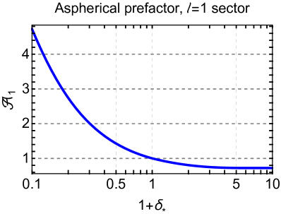
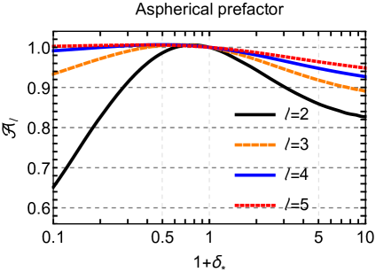
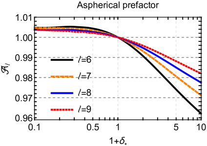
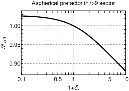
Figure 11 shows individual contributions of different multipoles to the aspherical prefactor. We fix the cell size to $r_{*}=10\,\text{Mpc}/h$; the results for $r_{*}=15\,\text{Mpc}/h$ are similar. The most significant contribution comes from the dipole sector and is shown in the upper left panel. We observe that it is a decreasing convex function that changes by a factor $\sim 0.2$ between $\delta_{*}=-0.9$ and $\delta_{*}=9$. At large $\delta_{*}$ the curve flattens out. The contributions of the multipoles with $2\leq\ell\leq 5$ and $6\leq\ell\leq 9$ are shown in the upper right and lower left panels respectively. These curves are quite different from the dipole: their deviation from unity in the explored $\delta_{*}$-range is only $\sim 40\%$ for the quadrupole and even less ($\lesssim 10\%$) for the higher multipoles. The variation of ${\cal A}_{\ell}$ decreases with the multipole number. Note that in the case of overdensities ($\delta_{*}>0$) all ${\cal A}_{\ell}$ are less than $1$ which is consistent with the expectation that any aspherical fluctuation makes collapse less efficient. On the other hand, at underdensities the partial contributions ${\cal A}_{\ell}$ can be both larger or smaller than unity, depending on the value of $\ell$.

The aggregate contribution of all sectors with $\ell>9$ is shown in the lower right panel of Fig. 11. It has been evaluated using the WKB formula (7.21). We test the validity of the WKB approximation by comparing it to the results of the full numerical routine in Fig. 12. The comparison is performed for $\ell=5$ (left panel) and $\ell=9$ (right panel). For $\ell=5$ there is a significant difference between the full calculation and the WKB approximation at strong underdensities. At overdensities the WKB approximation exhibits spurious wiggles that can be traced back to the baryon acoustic oscillations in the power spectrum. However, already for $\ell=9$ the WKB approximation is in perfect agreement with the full result. We have checked that the relative error introduced in the aggregate contribution of $\ell>9$ by the use of the WKB approximation does not exceed $10^{-3}$. Given that this contribution itself is small compared to that of lower multipoles, the error in the whole prefactor is negligible.

Figure 12: Comparison between the WKB approximation and the full numerical calculation for $\ell=5$ (left panel) and $\ell=9$ (right panel). The results are shown for $r_{*}=10$ Mpc/$h$.

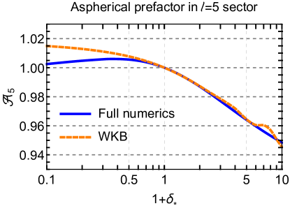
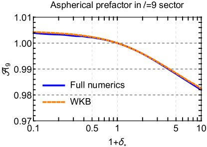
The total result for the aspherical prefactor obtained upon multiplying the contributions of all $\ell\geq 1$ is shown in Fig. 13, where it is compared with the prefactor extracted from the N-body data (see Sec. 3.2). One observes a good qualitative agreement between the theoretical curve and the data. However, there is a clear quantitative discrepancy which grows towards the edges of the $\delta_{*}$-interval. The discrepancy is somewhat bigger for $r_{*}=10\,\text{Mpc}/h$ than for $r_{*}=15\,\text{Mpc}/h$ and reaches $30\%$ ($100\%$) for underdense (overdense) tail. We interpret this discrepancy as the effect of short-scale physics that is not captured by the perfect-fluid hydrodynamics. In the next subsection we show how our results can be improved by renormalizing the contributions of short-scale modes.

Figure 13: The aspherical prefactor computed from fluctuation determinants (solid blue curve) against that extracted from the N-body simulations (black dots). The cell radii are $r_{*}=10\,\text{Mpc}/h$ (left panel) and $r_{*}=15\,\text{Mpc}/h$ (right panel).

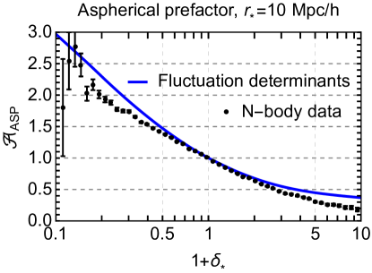
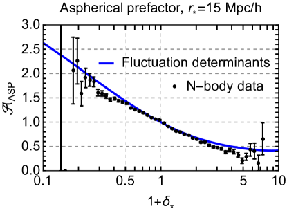
Let us make a comment. The fact that the fluctuation determinants found in our calculation are always positive provides a consistency check of the saddle-point approximation developed in Sec. 2. In particular, it shows that there are no other saddle points of the path integral (2.5) that would branch off the spherical collapse dynamics at any value of $\delta_{*}$ within the considered range. Indeed, if it were the case the spectrum of fluctuations around the spherical collapse at this value of $\delta_{*}$ would contain a zero mode, and hence at least one of the determinants ${\cal D}_{\ell}$ would vanish, which is not observed.

8.2 Renormalization of short-scale contributions

Up to this point we have worked within pressureless perfect fluid hydrodynamics, which is known to break down at short scales. This introduces an error in our calculation that must be corrected. A similar issue arises in the perturbative calculation of the density correlation functions in the homogeneous background where a systematic way to take into account the corrections due to UV modes is provided by introduction of counterterms in the hydrodynamics equations. These counterterms are constructed as a double expansion in the number of spatial derivatives acting on the fields and in the powers of the density contrast [18]. We have encountered this procedure in Sec. 4 where we made contact between the calculation of the prefactor at small density contrast and the calculation of 1-loop corrections to the power spectrum. At that level the sensitivity to the short-scale physics reduced to a single counterterm $\gamma(z)$, see Eq. (4.17).

The situation is more complicated at large density contrasts $\delta_{*}$ which we are interested in now. In this case, the evaluation of the aspherical prefactor can be viewed as a 1-loop calculation in the non-trivial background of the spherical collapse solution. Then the counterterm is, in general, a functional of the background, restricted by the symmetries of the problem, but otherwise arbitrary. It is impossible to rigorously fix its form without going beyond the EFT framework. In what follows we consider two schemes for renormalization of the aspherical prefactor that are based on reasonable physical assumptions. The difference between the two models should be treated as an intrinsic theoretical uncertainty of our current determination of ${\cal A}_{\rm ASP}$ due to the lack of control over the UV physics.

We start by analyzing the UV sensitivity of the aspherical prefactor. The contribution of modes with $k>k_{\rm UV}\gg 1/r_{*}$, $\ell\gg 1$ is described by the WKB expression (7.21). The sum over $\ell$ in the exponent can be rewritten as an integral,

$$\int_{k_{\rm UV}}^{\infty}\frac{dkP(k)}{(2\pi)^{3}}\sum_{\ell}\frac{1}{\ell+1/2}\;q\bigg{(}\frac{k}{\ell+1/2}\bigg{)} \simeq\int_{k_{\rm UV}}^{\infty}\frac{dkP(k)}{(2\pi)^{3}}\;\mathchoice{{\vbox{\hbox{$\textstyle-$}}\kern-4.86108pt}}{{\vbox{\hbox{$\scriptstyle-$}}\kern-3.25pt}}{{\vbox{\hbox{$\scriptscriptstyle-$}}\kern-2.29166pt}}{{\vbox{\hbox{$\scriptscriptstyle-$}}\kern-1.875pt}}\!\int\frac{d\ell}{\ell+1/2}\;q\bigg{(}\frac{k}{\ell+1/2}\bigg{)}$$

$$=\int_{k_{\rm UV}}^{\infty}\frac{dkP(k)}{(2\pi)^{3}}~{}\mathchoice{{\vbox{\hbox{$\textstyle-$}}\kern-4.86108pt}}{{\vbox{\hbox{$\scriptstyle-$}}\kern-3.25pt}}{{\vbox{\hbox{$\scriptscriptstyle-$}}\kern-2.29166pt}}{{\vbox{\hbox{$\scriptscriptstyle-$}}\kern-1.875pt}}\!\int\frac{d\varkappa}{\varkappa}\;q(\varkappa)\;.$$ (8.1)

We observe that the integral over momenta and the background dependence contained in the function $q$ factorize. In other words, all high-$k$ modes contribute into ${\cal A}_{\rm ASP}$ in a universal way. Of course, this is true only within the domain of validity of the formula (7.21) which neglects the interaction among the short modes and the departures from the hydrodynamic description. Precisely because of this inaccuracy, the integral over $k$ in (8.1) should be renormalized.

Figure 14: The counterterm prefactor for model 1 (left panel) and model 2 (right panel) evaluated for $\gamma_{0}=1.5$ (Mpc$/h$)², $z=0$ and cell radii $r_{*}=10$ Mpc$/h$ and $r_{*}=15$ Mpc$/h$.

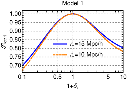
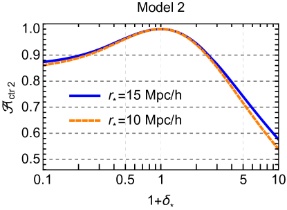
The integral in (8.1) is proportional to the high-$k$ contribution into the velocity dispersion

$$\sigma_{v}^{2}\equiv\frac{1}{6\pi^{2}}\int dk\,P(k)\;.$$ (8.2)

The same integral arises in the 1-loop correction to the power spectrum (see (4.22)) where it is renormalized by the substitution

$$\int\frac{dkP(k)}{(2\pi)^{3}}\mapsto\int\frac{dkP(k)}{(2\pi)^{3}}+\frac{315}{122\pi}\frac{\gamma(z)}{g^{2}(z)}\;.$$ (8.3)

We saw in Sec. 4.2 that this substitution also works for the aspherical prefactor at small $\delta_{*}$. Our first model for the renormalization of ${\cal A}_{\rm ASP}$ is obtained by extending the prescription (8.3) to finite values of $\delta_{*}$. It corresponds to an assumption that the main effect of renormalization in all quantities is the replacement of the tree-level velocity dispersion of high-$k$ modes with its renormalized value. For the redshift dependence of the counterterm we will use the scaling-universe approximation, as we did in Sec. 4.2. In this way we arrive at the following expression for the counterterm prefactor,

$$\mathcal{A}_{\text{ctr1}}=\exp\left(-\frac{315\gamma_{0}}{122\pi}\big{(}g(z)\big{)}^{-\frac{2(n+1)}{n+3}}\times 2\hat{\lambda}\int\frac{d\varkappa}{\varkappa}q(\varkappa)\right)\,,$$ (8.4)

where $\gamma_{0}$ is the 1-loop counterterm from the power spectrum and $n$ is the slope of the power spectrum at the mildly non-linear scales. For numerical estimates we will use $\gamma_{0}=1.5\,(\text{Mpc}/h)^{2}$, $n=-1.5$. The final answer for the aspherical prefactor is given by the product of (8.4) with the contribution obtained from the fluctuation determinants and described in the previous subsection. We will refer to the aspherical prefactor calculated using the counterterm (8.4) as “model 1”.

Figure 15: Upper panels: The aspherical prefactor in model 1 (dashed red curve) against the N-body data (black dots) for cell radii $r_{*}=10$ Mpc$/h$ (left panel) and $r_{*}=15$ Mpc$/h$ (right panel) at $z=0$. The aspherical prefactor without the counterterm is reproduced for comparison (solid blue curve). Lower panels: Residuals for the PDF extracted from the N-body data compared to our theoretical prediction at several redshifts for $r_{*}=10$ Mpc$/h$ (left panel) and $r_{*}=15$ Mpc$/h$ (right panel).

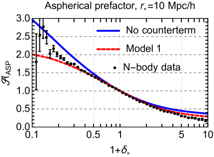
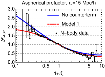
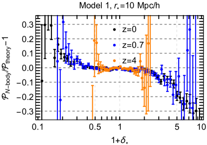
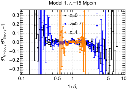
The counterterm prefactor (8.4) is plotted in the left panel of Fig. 14. We see that it captures the main qualitative features: it has a zero derivative at the origin where we expect the impact of shell-crossing to be negligible, and suppresses the probability for big under- and overdensities. In the upper panels of Fig. 15 we plot the aspherical prefactor in model 1 against the data. The aspherical prefactor without the counterterm is also shown for comparison. In the lower panels of Fig. 15 we show the residuals between the PDF measured from the N-body data and our theoretical template for several values of redshift. One observes a good agreement between the theory and the data. For $r_{*}=10\,\text{Mpc}/h$ the residuals are at sub-percent level in the range $-0.6<\delta_{*}<1$. They degrade to $10\%$ at $-0.8<\delta_{*}<-0.6$ and $1<\delta_{*}<3$. Eventually they increase to $\sim 30\%$ at the tails. Overall, the agreement is slightly better for the underdensities than for the overdensities. Similar trends are observed for $r_{*}=15\,\text{Mpc}/h$, though the precision of the N-body data is too low to see them unambiguously. It is worth noting that on general grounds one expects the effects of the UV physics to be weaker for larger cells.

As clear from Fig. 15, the model 1 systematically underestimates the aspherical prefactor for underdensities and overestimates for overdensities. This can be attributed to the following deficiency. We have taken the counterterm $\gamma$ to be independent of $\delta_{*}$. On the other hand, one expects the overdense regions to be more non-linear than the underdense ones, so that the effects of UV renormalization encapsulated by $\gamma$ should be larger (smaller) at $\delta_{*}>0$ ($\delta_{*}<0$) than at $\delta_{*}=0$. Comparing this with the formula (8.4) one sees that qualitatively such a dependence would act in the right direction to improve the agreement between the theory and the data.

Figure 16: Upper panels: The aspherical prefactor in model 2 (dashed red curve) against the N-body data (black dots) for cell radii $r_{*}=10$ Mpc$/h$ (left panel) and $r_{*}=15$ Mpc$/h$ (right panel) at $z=0$. The aspherical prefactor without the counterterm is reproduced for comparison (solid blue curve). Lower panels: Residuals for the PDF extracted from the N-body data compared to our theoretical prediction at several redshifts for $r_{*}=10$ Mpc$/h$ (left panel) and $r_{*}=15$ Mpc$/h$ (right panel).

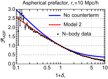
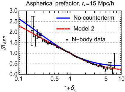
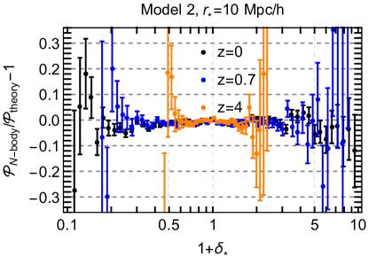
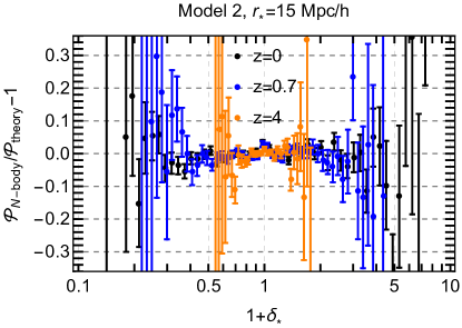
To estimate a possible effect of the $\delta_{*}$-dependence of $\gamma$, we use the following crude model. We approximate the spherical collapse solution by top-hat density profile with the final under-/over-density $\delta_{*}$. Treating such a profile as an open/closed separate universe, we replace the counterterm and the growth factor in Eq. (8.3) by $\gamma(\delta_{*},z)$ and $D(\delta_{*},z)$ — the counterterm and the growth factor in the separate universe. The latter is derived in Appendix C.4. To estimate $\gamma(\delta_{*},z)$ we again use the power-law approximation for the power spectrum and obtain $\gamma(\delta_{*},z)\propto\big{(}D(\delta_{*},z)\big{)}^{\frac{4}{n+3}}$. All in all, this leads to the replacement of $g(z)$ in the counterterm prefactor (8.4) by the density-dependent growth factor $D(\delta_{*},z)$. Using the explicit expression for the latter, Eq. (C.39), we obtain model 2 for the counterterm,

$$\mathcal{A}_{\text{ctr2}}=\exp\left(-\frac{315\gamma_{0}}{122\pi}\Big{(}\frac{g(z)}{F^{\prime}(\delta_{*})(1+\delta_{*})}\Big{)}^{-\frac{2(n+1)}{n+3}}\times 2\hat{\lambda}\int\frac{d\varkappa}{\varkappa}q(\varkappa)\right)\,,$$ (8.5)

This counterterm prefactor is shown in the right panel of Fig. 14. Compared to the model 1, it gives less suppression at underdensities and stronger suppresses overdensities. In the upper panels of Fig. 16 we compare the aspherical prefactor in model 2 with the N-body data and the prefactor without the counterterm. In the lower panels of Fig. 16 we show the residuals between the PDF measured from the N-body data and our theoretical template for $z=0$, $0.7$, $4$. One observes an excellent agreement between the theory and the data within the precision of the latter. This is striking given the crudeness of the model.

We leave a detailed investigation of the counterterms in the spherical collapse background for future and propose to treat the difference between the models 1 and 2 as a proxy for the theoretical uncertainty. Notice that this uncertainty estimate is internal to the theoretical approach and does not require any comparison with N-body simulations. We also emphasize that none of the two counterterm models proposed in this section introduces any additional fitting parameter, as the coefficient $\gamma_{0}$ entering in Eqs. (8.4), (8.5) must be the same as the one measured from the dark matter power spectrum.

9 Summary and Discussion

In this paper we computed the 1-point probability distribution function (PDF) of the cosmic matter density field in spherical cells. Our approach makes use of the path integral description of large-scale structure. We identified the saddle point of the path integral that corresponds to the spherical collapse dynamics and yields the leading exponent of the PDF. Then we computed the prefactor given by the determinant of the quadratic fluctuations around the saddle-point solution. This can be viewed as a 1-loop calculation in perturbation theory around a fully non-linear background.

We showed that the prefactor factorizes into the contributions of fluctuations in different multipole sectors and evaluated the monopole contribution exactly. Next we considered the contribution of fluctuations with $\ell>0$ which we called ‘the aspherical prefactor’ ${\cal A}_{\rm ASP}$. We demonstrated that it is crucial for the consistency of the PDF, in particular, for ensuring that the mean density contrast evaluated using the PDF vanishes. Our final formula for the 1-point PDF has the form,

$$\mathcal{P}(\delta_{*})={\cal A}_{\rm ASP}(\delta_{*})\frac{\hat{C}(\delta_{*})}{\sqrt{2\pi g^{2}\sigma^{2}_{R_{*}}}}{\rm e}^{-\frac{F^{2}(\delta_{*})}{2g^{2}\sigma^{2}_{R_{*}}}}\,,$$ (9.1)

where $g(z)$ is the linear growth factor, $\sigma_{R_{*}}$ is the linear density variance at $z=0$ filtered at the Lagrangian radius $R_{*}=r_{*}(1+\delta_{*})^{1/3}$, $F(\delta_{*})$ is the linear overdensity corresponding to $\delta_{*}$ through the spherical collapse mapping, and the function $\hat{C}(\delta_{*})$ is defined by the formula (2.29).

We computed the aspherical prefactor using several techniques. First, we treated the background perturbatively, which allowed us to capture the correct shape of the prefactor for small averaged densities. Second, we computed the partial contributions to the prefactor from sectors with high orbital numbers treating the background non-perturbatively. We showed that this limit allows one to use the WKB technique, which made possible a semi-analytic treatment of the problem. Finally, we developed a numerical procedure for a fully non-linear computation of the aspherical determinant on the grid. This procedure includes analytic factorization and cancellation of the so-called ‘IR-divergences’ — spurious enhanced contributions that appear in the dipole sector and are associated with large bulk flows. We implemented this procedure in an open-source Python code AsPy available at the following link [61].

Figure 17: 1-point probability distribution function computed in this work (blue band) against that extracted from our N-body data (black dots). The results are presented for redshift zero, $z=0$, and two cell radii, $r_{*}=10\,\text{Mpc}/h$ (left panel) and $r_{*}=15\,\text{Mpc}/h$ (right panel). The width of the theoretical band is set by the uncertainty in modelling the short-distance physics; it exceeds the line width only at the tails of the distribution.

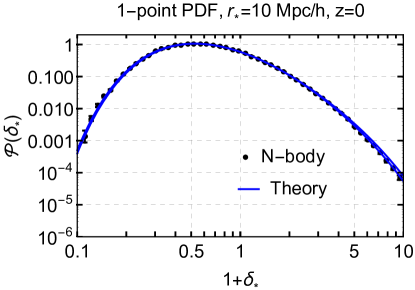
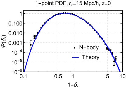
We compared the results of our computation to the N-body data. Despite a qualitative agreement, we observed a sizable quantitative discrepancy, which we attributed to the failure of the pressureless fluid approximation at short scales. We proposed two models for renormalization of the short-scale contributions in the spirit of the EFT of LSS. The two models agree at the percent level at moderate density contrasts and deviate by at most $30\%$ at the tails of the distribution. We have suggested to use the difference between the two models as an estimate of the theoretical uncertainty of our approach stemming from the lack of control over the short-distance physics.

The resulting theoretical PDFs for cells with radii $r_{*}=10\,\text{Mpc}/h$ and $15\,\text{Mpc}/h$ at $z=0$ are shown against N-body data in Fig. 17. The lines corresponding to the two counterterm models are almost indistinguishable. We see that the theory and the data are in excellent agreement. The theoretical uncertainty is smaller for the larger radius, which is consistent with the expectation that the UV effects should be suppressed at large distances.

The 1-point PDF has a very distinctive sensitivity to the dynamics and initial statistics of the matter density perturbations. One observes from Eq. (9.1) that the dependence of the PDF on the filtered linear density variance $g\sigma_{R_{*}}$ factorizes. By varying $\delta_{*}$ one effectively changes the filtering radius, and thus probes the variance of the density field at different scales. Going to the underdense tail allows one to test the linear power spectrum at very small Lagrangian radii, i.e. at the scales which are beyond the regime of validity of the standard cosmological perturbation theory.

We have shown that the prefactor in (9.1) has only a weak dependence on cosmology. Thus, any variation of the cosmological parameters or extension of $\Lambda$CDM is expected to affect the PDF primarily through the leading exponent. Even a small change in the growth factor or the linear variance can have a strong effect on the PDF. On the other hand, the sensitivity to the non-linear dynamics at leading order is encoded in the spherical collapse mapping $F(\delta_{*})$. It will be interesting to understand to which extent this property of the 1-point PDF can be used to constrain non-standard dark matter scenarios or modifications of gravity.

The expansion parameter in our approach is the linear density variance smoothed at the scale of the window function. Thus, corrections to our result for the aspherical prefactor are expected to scale as $(g\sigma_{r_{*}})^{2}$, c.f. Eq. (2.8). On the other hand, our comparison with the N-body data has not revealed any presence of such corrections for $(g\sigma_{r_{*}})^{2}$ as large as $\sim 0.5$ (for $z=0$, $r_{*}=10$Mpc$/h$, see Table 1). This indicates that the coefficient in front of the correction is suppressed. Nevertheless, as one decreases the cell radius, the corrections will grow and eventually the ‘semiclassical’ approximation is expected to break down. Another limitation of our method in its present form is its reliance on the existence of an analytic spherical collapse saddle-point solution. As discussed in Sec. 2.2, this assumption is actually violated for large overdensities $\delta_{*}\gtrsim 7$ where the saddle-point solution exhibits shell crossing. Remarkably, the N-body data still obey the ‘semiclassical’ scaling up to the maximal value $\delta_{*}=9$ that we were able to explore. We have interpreted it as a consequence of the slow signal propagation in dark matter which implies that the information about the shell crossing in the inner part of the density profile does not have enough time to reach the boundary of the cell. However, an extension to yet higher overdensities will likely require a modification of the semiclassical method to properly take the shell crossing into account, cf. [47]. It would be highly instructive to map the domain of validity of the ‘semiclassical’ formula (9.1) in the space of cell radii $r_{*}$ and densities $\delta_{*}$ using high-precision counts-in-cells statistics obtained from state of the art cosmological simulations.

Let us briefly comment on the relation between the PDF derived in this work and the log-normal distribution that has been widely used in the literature to model the counts-in-cells statistics. As discussed in Appendix H, the success of the log-normal model does not appear to have any physical meaning, but is a consequence of an accidental conspiracy between the spherical collapse dynamics and the shape of the power spectrum in our universe, that makes the combination $F(\delta_{*})/\sigma_{R_{*}}$ entering in the exponent of (9.1) look similar to $\mathop{\rm ln}\nolimits(1+\delta_{*})/\sigma_{\rm ln}$, where $\sigma_{\rm ln}$ is the log-density variance. A change of the slope of the power spectrum would destroy this conspiracy. Even for the standard $\Lambda$CDM the approximation of $F/\sigma_{R_{*}}$ by the logarithm does not work for large under- and over-densities. Moreover, the log-normal model does not incorporate the correct prefactor. As a result, it significantly deviates from the N-body data in the tails of the distribution (cf. Refs. [31, 42]).

Before concluding, we summarize several key features of our approach:

1. It clearly separates the leading exponent from the prefactor. This allows us to keep the saddle-point expansion under control and disentangle the cosmology-dependent effects from those of non-linear clustering.

2. We use the exact $\Lambda$CDM mapping for spherical collapse. This is crucial for the accuracy of our calculation, as the PDF is exponentially sensitive to the mapping.

3. It explicitly takes into account aspherical fluctuations along with the contributions beyond the single-stream pressureless perfect fluid approximation.

4. It is based on the first principles and does not introduce any fitting parameters.

5. It provides an intrinsic estimate of the theoretical uncertainty that does not require an input from the N-body data.

6. It increases the range of agreement between the analytic theory and N-body simulations compared to previous approaches.

In this paper we have studied the simplest case of non-perturbative cosmological statistics: 1-point PDF of dark matter in real space for Gaussian adiabatic initial conditions. Applications to realistic observations, such as galaxy surveys, Lyman-$\alpha$ forest or 21 cm intensity mapping will require extension of the method to the biased tracers in redshift space. Another line of research is the statistics of the 2-dimensional projected density field and weak lensing convergence. Last but not least, a generalization to the 2-point PDF will be very interesting as a way to probe the primordial non-Gaussianity. We believe that our study paves the way for a systematic investigation these non-perturbative statistics as potentially powerful cosmological probes.

Acknowledgments

We are indebted to Cora Uhlemann for stimulating discussions and comments on the draft. We thank D. Blas, S. Dubovsky, S. Foreman, M. Garny, J. Garcia-Bellido, M. Mirbabayi, L. Hui, F. Popov, F. Schmidt, M. Schmittfull, M. Simonović, A. Shkerin, P. Valageas, Z. Vlah and M. Zaldarriaga for fruitful conversations and ecouraging interest. The numerical part of this work was done on the Helios cluster at the Institute for Advanced Study. The work of M.I. and S.S. is supported by the Swiss National Science Foundation. A.K. is supported by the William D. Loughlin Membership Fund. M.I. also acknowledges a partial support by the RFBR grant No. 17-02-01008. S.S. is supported by the RFBR grant No. 17-02-00651.

Appendix A Conventions

In this Appendix we summarize our main notations and conventions. The Fourier transform is defined as,

$$\delta({\bf x})=\int_{\bf k}\delta({\bf k}){\rm e}^{i{\bf k}\cdot{\bf x}}\,,$$ (A.1)

where the integration measure in momentum space is

$$\int_{\bf k}=\int\frac{d^{3}k}{(2\pi)^{3}}\;.$$ (A.2)

We also use the shorthand notation for the radial integral in momentum space,

$$\int[dk]=\int_{0}^{\infty}\frac{k^{2}dk}{(2\pi)^{3}}\;,$$ (A.3)

and its generalization to several wavenumbers,

$$\int[dk]^{n}=\int\prod_{i=1}^{n}\frac{k^{2}_{i}dk_{i}}{(2\pi)^{3}}\;,$$ (A.4)

The power spectrum is defined as,

$$\langle\delta({\bf k})\delta({\bf k}^{\prime})\rangle=(2\pi)^{3}\delta_{\rm D}^{(3)}({\bf k}+{\bf k}^{\prime})P(k)\,,$$ (A.5)

where $\delta_{\rm D}^{(d)}({\bf k})$ is the Dirac delta-function in a $d$-dimensional space.

We use the following definition for the spherical harmonics:

$$Y_{0}(\theta,\phi)=1\;,$$ (A.6a)

$$Y_{\ell m}(\theta,\phi)=\frac{(-1)^{\ell+m}}{2^{\ell}\ell!}\bigg{[}\frac{2\ell+1}{4\pi}\frac{(\ell-|m|)!}{(\ell+|m|)!}\bigg{]}^{1/2}{\rm e}^{im\phi}(\sin\theta)^{|m|}\bigg{(}\frac{d}{d\cos\theta}\bigg{)}^{\ell+|m|}(\sin\theta)^{2\ell},$$

$$\qquad\qquad\qquad\ell>0\;,~{}~{}~{}~{}-\ell<m<\ell\;.$$ (A.6b)

They obey the relations,

$$\Delta_{\Omega}Y_{\ell m}=-\ell(\ell+1)Y_{\ell m}~{},~{}~{}~{}~{}Y_{\ell m}(-{\bf n})=(-1)^{\ell}Y_{\ell m}({\bf n})~{},~{}~{}~{}~{}Y_{\ell m}^{*}({\bf n})=Y_{\ell,-m}({\bf n})\;,$$ (A.7)

where $\Delta_{\Omega}$ is the Laplacian on a unit 2-dimensional sphere. All harmonics are orthogonal and normalized to 1 when integrated over a 2d sphere, except the monopole that has the norm $4\pi$,

$$\int d\Omega\,Y_{\ell m}\,Y^{*}_{\ell^{\prime}m^{\prime}}=(4\pi)^{\delta_{0\ell}}\delta_{\ell\ell^{\prime}}\delta_{mm^{\prime}}\,,$$ (A.8)

where $\delta_{ij}$ is the Kronecker delta symbol. Note that our definition (A.6b) differs by a factor $(-1)^{\frac{m-|m|}{2}}$ from the standard conventions [60].

We expand the fields over spherical harmonics in position and Fourier space as,

$$\delta({\bf x})=\delta_{0}(r)+\sum_{\ell>0}\sum_{m=-\ell}^{\ell}\delta_{\ell m}(r)\,Y_{\ell m}({\bf x}/r)\;,$$ (A.9a)

$$\delta({\bf k})=\delta_{0}(k)+\sum_{\ell>0}\sum_{m=-\ell}^{\ell}(-i)^{\ell}\,\delta_{\ell m}(k)\,Y_{\ell m}({\bf k}/k)\;.$$ (A.9b)

Due to the relations (A.7) we have,

$$\big{(}\delta_{\ell m}(r)\big{)}^{*}=\big{(}\delta_{\ell,-m}(r)\big{)}~{},~{}~{}~{}~{}~{}~{}\big{(}\delta_{\ell m}(k)\big{)}^{*}=\big{(}\delta_{\ell,-m}(k)\big{)}\;.$$ (A.10)

The coefficient functions in the above expansions are related by,

$$\delta_{\ell m}(r)=4\pi\int[dk]\;j_{\ell}(kr)\,\delta_{\ell m}(k)\,,$$ (A.11)

where $j_{\ell}(x)$ is the spherical Bessel function of order $\ell$. It is related to the Bessel function of the first kind via

$$j_{\ell}(x)=\sqrt{\frac{\pi}{2x}}J_{\ell+1/2}(x)\,.$$ (A.12)

The first few functions are,

$$j_{0}(x)=\frac{\sin x}{x}~{},~{}~{}~{}~{}j_{1}(x)=\frac{\sin x}{x^{2}}-\frac{\cos x}{x}~{},~{}~{}~{}~{}j_{2}(x)=\bigg{(}-\frac{1}{x}+\frac{3}{x^{3}}\bigg{)}\sin x-\frac{3}{x^{2}}\cos x\;.$$ (A.13)

Spherical Bessel functions $j_{\ell}(kr)$ with different arguments $k$ form an orthogonal basis on the half-line with the normalization

$$\int_{0}^{\infty}dr\,r^{2}j_{\ell}(k^{\prime}r)j_{\ell}(kr)=\frac{\pi}{2k^{2}}\delta_{\rm D}^{(1)}(k-k^{\prime})\,.$$ (A.14)

They are eigenmodes of the radial part of the Laplace operator,

$$\partial_{r}^{2}j_{\ell}(kr)+\frac{2}{r}\partial_{r}j_{\ell}(kr)-\frac{\ell(\ell+1)}{r^{2}}j_{\ell}(kr)=-k^{2}j_{\ell}(kr)\;.$$ (A.15)

Appendix B Description of N-body data

We use the data on the counts-in-cells 1-point PDF extracted from the N-body simulations run with the FastPM code [51]. To generate these data we simulated $300$ boxes with $L_{\text{box}}=256$ Mpc/$h$ on a side, totaling the volume of $5~{}(\text{Gpc}/h)^{3}$. The number of dark matter particles per box is $1024^{3}$, corresponding to mass resolution $1.1\cdot 10^{9}~{}M_{\odot}/h$. The adopted force resolution is half the mean of the dark matter particle separation $\sim 125$ kpc$/h$. The boxes are initialized at $z=99$ with second-order Lagrangian perturbation theory (2LPT), and then evolved to $z=0$ using the FastPM integration scheme and 40 linearly spaced in scale factor time steps. We assumed a flat $\Lambda$CDM with $\Omega_{m}=0.26$, $\Omega_{b}=0.044$, $h=0.72$, $n_{s}=0.96$, Gaussian initial conditions, $\sigma_{8}=0.794$. The input linear power spectrum was generated with the Boltzmann code CLASS [53].

For each box we saved snapshots taken at $z=0,~{}0.7,~{}4$ and extracted $12^{3}$ non-overlapping $r_{*}=10$ Mpc$/h$ (518400 in total) and $8^{3}$ $r_{*}=15$ Mpc$/h$ spheres (153600 in total) centered on a regular grid with $2r_{*}$ spacing. The data shown in this paper were binned in $\sim 50$ logarithmically-spaced intervals spanning the range $1+\delta_{*}=[0.1,10]$. When comparing the data against theory, we also integrate the theoretical predictions within corresponding bin intervals. The data errors shown correspond to the Poissonian standard deviation.

The counterterm $\gamma_{0}$ is measured from the non-linear dark matter power spectrum of the Horizon Run 2 simulation (HR2) [52], whose cosmology is identical to ours. The HR2 simulation box ($L_{\text{box}}=7.2$ Gpc/$h$) is significantly larger than the one of our simulations, and therefore allows for a very precise measurements of $\gamma_{0}$, which is important for the accuracy of our theoretical prediction. We also estimated the non-linear dark matter power spectrum of our simulations using the nbodykit toolkit [62], and found that it is consistent with HR2 within statistical errors within interesting range of $k$.

The simulations used in this paper compromise on accuracy in order to produce large statistics given limited computational resources available to us. Thus, they are much less accurate than the state-of-the-art simulations such as reported in Ref. [31]. In particular, our experiments show that numerical effects such as force resolution, super-sample variance and particle counts are not negligible. They have a noticeable effect on the tails of the counts-in-cells probability distribution. Our experiments suggest that the systematic numerical errors are comparable to the statistical ones for the most over(under)-dense bins, whose comparison with theory should be taken with a grain of salt. We plan to use more accurate N-body simulations for an exhaustive precision comparison in the future.

Appendix C Dynamics of spherical collapse

C.1 Spherical collapse in Einstein–de Sitter universe

Consider a spherically symmetric density perturbation in a spatially flat universe filled with non-relativistic matter. For concreteness, we focus on the case of an overdensity. We study the motion of a spherical shell of matter enclosing the total mass $M$. Before the onset of shell-crossing the mass within the shell is conserved. Due to Newton’s theorem (or Birkhoff’s theorem in general relativity) the mechanical energy of the shell is conserved, so we write,

$$\frac{1}{2}\left(\frac{dy}{d\tau}\right)^{2}-\frac{GM}{y}={\cal E}\,,$$ (C.1)

where $y$ is the physical radius of the shell and $\tau$ is the physical time. The conserved energy ${\cal E}$ is negative for the case of an overdensity. It is straightforward to obtain the solution to (C.1) in a parametric form,

$$y=-\frac{GM}{2{\cal E}}(1-\cos\theta)\;,$$ (C.2a)

$$\tau=\frac{GM}{(-2{\cal E})^{3/2}}(\theta-\sin\theta)\;.$$ (C.2b)

Next, we switch from the variables $y$, $\tau$ to the comoving radius of the shell $r=y/a$ and the scale factor $a$. We use,

$$a=\bigg{(}\frac{8\pi G}{3}\rho_{i}a_{i}^{3}\bigg{)}^{1/3}\bigg{(}\frac{3}{2}\tau\bigg{)}^{2/3}\;,$$ (C.3)

$$M=\frac{4\pi}{3}\rho_{i}a_{i}^{3}R^{3}\;,$$ (C.4)

where $\rho_{i}$, $a_{i}$ and $R$ are the matter density, the scale factor and the comoving radius of the shell at some early time when the universe was almost homogeneous. Note that $R$ has a finite limit at $a_{i}\to 0$ which coincides with the Lagrangian radius of the shell. Substitution of (C.3), (C.4) into Eqs. (C.2), gives,

$$r=R\bigg{(}\frac{2}{9}\bigg{)}^{1/3}\frac{1-\cos\theta}{(\theta-\sin\theta)^{2/3}}\;,$$ (C.5a)

$$a=\bigg{(}\frac{9}{2}\bigg{)}^{1/3}\frac{4\pi G}{3(-2{\cal E})}\rho_{i}a_{i}^{3}R^{2}(\theta-\sin\theta)^{2/3}\;,$$ (C.5b)

We now recall the definition of the spherically averaged density contrast (2.11). Expressing it through the enclosed mass $M$, the radius of the shell and the mean density of the universe $\rho_{\rm univ}$ we obtain,

$$1+\bar{\delta}(r)=\frac{3M}{4\pi y^{3}\rho_{\rm univ}}=\bigg{(}\frac{R}{r}\bigg{)}^{3}\;,$$ (C.6)

where in the second equality we used that $\rho_{\rm univ}=\rho_{i}a_{i}^{3}/a^{3}$. This gives the relation (2.13) between the Lagrangian and Eulerian radii of the shell. Besides, we have from (C.5a),

$$\bar{\delta}={\cal F}(\theta)~{},~{}~{}~{}~{}\text{where}~{}~{}{\cal F}(\theta)\equiv\frac{9}{2}\frac{(\theta-\sin\theta)^{2}}{(1-\cos\theta)^{3}}-1\,.$$ (C.7)

It remains to relate the constant ${\cal E}$ to the initial overdensity. To this end, we consider Eqs. (C.5b), (C.7) at the initial time. The parameter $\theta$ is initially small, so we can expand,

$$a_{i}=\frac{\theta_{i}^{2}}{2}\frac{4\pi G}{3(-2{\cal E})}\rho_{i}a_{i}^{3}R^{2}~{},~{}~{}~{}~{}~{}~{}~{}\bar{\delta}_{i}(R)=\frac{3}{20}\theta_{i}^{2}\;,$$ (C.8)

which gives

$${\cal E}=-\frac{5}{3}\,\frac{\bar{\delta}_{i}(R)}{a_{i}}\,\frac{4\pi G}{3}\rho_{i}a_{i}^{3}R^{2}\;.$$ (C.9)

Substituting ${\cal E}$ back into (C.5b) and introducing the rescaled linear density contrast $\bar{\delta}_{L}(R)\equiv a\bar{\delta}_{i}(R)/a_{i}$ we arrive at

$$\bar{\delta}_{L}(R)={\cal G}(\theta)\equiv\frac{3}{20}[6(\theta-\sin\theta)]^{2/3}\,.$$ (C.10)

Equations (C.7), (C.10) together provide a mapping between the linear and non-linear averaged density contrasts at a given moment of time expressed parametrically through the so-called development angle $\theta$. The functions $f$ and $F$ used in the main text (see Eq. (2.14)) are the superpositions

$$f={\cal F}\circ{\cal G}^{-1}~{},~{}~{}~{}~{}~{}F={\cal G}\circ{\cal F}^{-1}\;.$$ (C.11)

We now derive several useful expressions for the fields characterizing the spherical collapse that are required for the calculation of linear fluctuations around the spherical collapse saddle point in Sec. 5. It is convenient to choose the logarithm of the growth factor as a new time variable,

$$\eta=\mathop{\rm ln}\nolimits a\;.$$ (C.12)

The key object is the linear density profile which we rescale to zero redshift. This will be denoted by $\delta_{L|0}(R)$. All other quantities are sourced by it and should be understood as functions of $\eta$ and $R$. We first rewrite (C.10)

$$\theta-\sin\theta=\frac{{\rm e}^{3\eta/2}}{6}\bigg{(}\frac{20}{3}\,\bar{\delta}_{L|0}(R)\bigg{)}^{3/2}\;,$$ (C.13a)

which implicitly defines the function $$\theta(\eta,R)$$. Then we obtain the relations,

$$\frac{\partial\theta}{\partial R}=\frac{3(\theta-\sin\theta)}{2(1-\cos\theta)}\cdot\frac{\bar{\delta}^{\prime}_{L|0}(R)}{\bar{\delta}_{L|0}(R)}~{},~{}~{}~{}~{}~{}~{}~{}~{}~{}~{}~{}\frac{\partial\theta}{\partial\eta}=\frac{3(\theta-\sin\theta)}{2(1-\cos\theta)}~{},$$ (C.13b)

$$\frac{\partial r}{\partial R}=\bigg{(}\frac{2}{9}\bigg{)}^{1/3}\frac{1-\cos\theta}{(\theta-\sin\theta)^{2/3}}\bigg{[}1+R\frac{\bar{\delta}_{L|0}^{\prime}}{\bar{\delta}_{L|0}}\bigg{(}\frac{3(\theta-\sin\theta)\sin\theta}{2(1-\cos\theta)^{2}}-1\bigg{)}\bigg{]}\;,$$ (C.13c)

which yield the overdensity field,

$$\delta=\bigg{[}\frac{r^{2}}{R^{2}}\frac{\partial r}{\partial R}\bigg{]}^{-1}-1=\frac{9(\theta-\sin\theta)^{2}}{2(1-\cos\theta)^{3}}\bigg{[}1+R\frac{\bar{\delta}_{L|0}^{\prime}}{\bar{\delta}_{L|0}}\bigg{(}\frac{3(\theta-\sin\theta)\sin\theta}{2(1-\cos\theta)^{2}}-1\bigg{)}\bigg{]}^{-1}-1\,.$$ (C.13d)

We also need the velocity potential $$\Psi$$ defined as

$$\partial_{r}\Psi=-u_{r}/{\cal H}\;,$$

where $$u_{r} u_{r}=\frac{\partial r}{\partial t} {\cal H}=\frac{1}{a}\frac{da}{dt} t$$ is the radial velocity of collapsing matter, , and . Here is the conformal time. We obtain,

$$\partial_{r}\Psi=-\frac{\partial r}{\partial\eta}=-R\bigg{(}\frac{2}{9}\bigg{)}^{1/3}\frac{1-\cos\theta}{(\theta-\sin\theta)^{2/3}}\bigg{[}\frac{3(\theta-\sin\theta)\sin\theta}{2(1-\cos\theta)^{2}}-1\bigg{]}\;.$$ (C.13e)

Finally, the rescaled velocity divergence is

$$\Theta\equiv-\frac{\partial_{i}u_{i}}{\cal H}=\bigg{(}\frac{\partial r}{\partial R}\bigg{)}^{-1}\frac{\partial}{\partial R}\partial_{r}\Psi+\frac{2}{r}\partial_{r}\Psi\;.$$ (C.13f)

In the case of an underdensity, the spherically symmetric dynamics is similar with only minor modifications. Without repeating the analysis, we summarize the relevant expressions,

$${\cal G}(\theta)=\frac{3}{20}[6(\mathop{\rm sh}\nolimits\theta-\theta)]^{2/3}\,,\qquad{\cal F}(\theta)=\frac{9(\mathop{\rm sh}\nolimits\theta-\theta)^{2}}{2(\mathop{\rm ch}\nolimits\theta-1)^{3}}-1\,,$$ (C.14a)

$$\mathop{\rm sh}\nolimits\theta-\theta=\frac{{\rm e}^{3\eta/2}}{6}\bigg{(}-\frac{20}{3}\bar{\delta}_{L|0}(R)\bigg{)}^{3/2}\;,$$ (C.14b)

$$\frac{\partial\theta}{\partial R}=\frac{3(\mathop{\rm sh}\nolimits\theta-\theta)}{2(\mathop{\rm ch}\nolimits\theta-1)}\frac{\bar{\delta}_{L|0}^{\prime}}{\bar{\delta}_{L|0}}\;,\qquad\frac{\partial\theta}{\partial\eta}=\frac{3(\mathop{\rm sh}\nolimits\theta-\theta)}{2(\mathop{\rm ch}\nolimits\theta-1)}\;,$$ (C.14c)

$$r=R\bigg{(}\frac{2}{9}\bigg{)}^{1/3}\frac{\mathop{\rm ch}\nolimits\theta-1}{(\mathop{\rm sh}\nolimits\theta-\theta)^{2/3}}\;,$$ (C.14d)

$$\frac{\partial r}{\partial R}=\bigg{(}\frac{2}{9}\bigg{)}^{1/3}\frac{\mathop{\rm ch}\nolimits\theta-1}{(\mathop{\rm sh}\nolimits\theta-\theta)^{2/3}}\bigg{[}1+R\frac{\bar{\delta}_{L|0}^{\prime}}{\bar{\delta}_{L|0}}\bigg{(}\frac{3(\mathop{\rm sh}\nolimits\theta-\theta)\mathop{\rm sh}\nolimits\theta}{2(\mathop{\rm ch}\nolimits\theta-1)^{2}}-1\bigg{)}\bigg{]}\;,$$ (C.14e)

$$\delta=\frac{9(\mathop{\rm sh}\nolimits\theta-\theta)^{2}}{2(\mathop{\rm ch}\nolimits\theta-1)^{3}}\bigg{[}1+R\frac{\bar{\delta}_{L|0}^{\prime}}{\bar{\delta}_{L|0}}\bigg{(}\frac{3(\mathop{\rm sh}\nolimits\theta-\theta)\mathop{\rm sh}\nolimits\theta}{2(\mathop{\rm ch}\nolimits\theta-1)^{2}}-1\bigg{)}\bigg{]}^{-1}-1\;,$$ (C.14f)

$$\partial_{r}\hat{\Psi}=-R\bigg{(}\frac{2}{9}\bigg{)}^{1/3}\frac{\mathop{\rm ch}\nolimits\theta-1}{(\mathop{\rm sh}\nolimits\theta-\theta)^{2/3}}\bigg{[}\frac{3(\mathop{\rm sh}\nolimits\theta-\theta)\mathop{\rm sh}\nolimits\theta}{2(\mathop{\rm ch}\nolimits\theta-1)^{2}}-1\bigg{]}\;.$$ (C.14g)

C.2 Spherical collapse in $\Lambda$CDM

Here we discuss how the previous results are modified in $\Lambda$CDM. In the presence of a cosmological constant $\Lambda$ the equation (C.1) for the trajectory of a spherical shell is replaced by [63, 64],

$$\frac{1}{2}\left(\frac{dy}{d\tau}\right)^{2}-\frac{GM}{y}-\frac{\Lambda y^{2}}{6}={\cal E}\,.$$ (C.15)

Unlike Eq. (C.1), this cannot be solved analytically, so one has to resort to numerical integration. It is convenient to use the scale factor $a$ as the time variable and switch from $y$ to the variable

$$\zeta\equiv R/r\;,$$ (C.16)

where $r=y/a$ and $R=\lim_{a\to 0}r$. One uses the Hubble equation,

$$\frac{1}{a^{2}}\bigg{(}\frac{da}{d\tau}\bigg{)}^{2}=\frac{8\pi G}{3}\rho_{\rm univ}+\frac{\Lambda}{3}\;,$$ (C.17)

and the relations $\rho_{\rm univ}=\rho_{0}/a^{3}$, $\Lambda=8\pi G\rho_{0}\Omega_{\Lambda}/\Omega_{m}$, with $\rho_{0}$ the present-day average matter density and $\Omega_{\Lambda}=1-\Omega_{m}$. Then Eq. (C.15) takes the following form,

$$\bigg{(}1-\frac{d\mathop{\rm ln}\nolimits\zeta}{d\mathop{\rm ln}\nolimits a}\bigg{)}^{2}=\bigg{(}1+\frac{\Omega_{\Lambda}}{\Omega_{m}}a^{3}\bigg{)}^{-1}\bigg{(}\zeta^{3}+\frac{\Omega_{\Lambda}}{\Omega_{m}}a^{3}+\frac{3{\cal E}}{4\pi G\rho_{0}R^{2}}\,a\zeta^{2}\bigg{)}\;.$$ (C.18)

To fix the value of the energy ${\cal E}$, we observe that Eq. (C.6) still applies in $\Lambda$CDM, so we have,

$$1+\bar{\delta}(r)=\zeta^{3}\;,$$ (C.19)

which at early times gives $\zeta=1+\big{(}a\bar{\delta}_{i}(R)\big{)}/(3a_{i})$. Substituting this into (C.18) and matching terms linear in $a$ at $a\to 0$, we recover the same expression for ${\cal E}$, as in the EdS case,

$$\frac{3{\cal E}}{4\pi G\rho_{0}R^{2}}=-\frac{5}{3}\frac{\bar{\delta}_{i}(R)}{a_{i}}\;.$$ (C.20)

The next step is to express the initial overdensity in terms of the linear density contrast $\bar{\delta}_{L}(R)$ at the redshift $z$, at which we want to establish the spherical collapse mapping. To this end we write,

$$\frac{\bar{\delta}_{i}(R)}{a_{i}}=\frac{g(z)}{g(z_{i})}\bar{\delta}_{i}(R)\,\frac{g(z_{i})}{a_{i}}\,\frac{1}{g(z)}=\frac{g_{\Lambda}}{g(z)}\bar{\delta}_{L}(R)\;.$$ (C.21)

In the last equality we have used that at early times the growth factor is proportional to $a$,

$$g(z_{i})=g_{\Lambda}\cdot a_{i}\,$$ (C.22)

where $g_{\Lambda}$ is a constant. Collecting the relations (C.20), (C.21) and inserting them into Eq. (C.18) we cast the latter in the form,

$$\bigg{(}1-\frac{d\mathop{\rm ln}\nolimits\zeta}{d\mathop{\rm ln}\nolimits a}\bigg{)}^{2}=\bigg{(}1+\frac{\Omega_{\Lambda}}{\Omega_{m}}a^{3}\bigg{)}^{-1}\bigg{(}\zeta^{3}-\frac{5g_{\Lambda}}{3g(z)}\bar{\delta}_{L}(R)\,a\zeta^{2}+\frac{\Omega_{\Lambda}}{\Omega_{m}}a^{3}\bigg{)}\;.$$ (C.23)

With this in hand, the algorithm to construct the spherical collapse mapping goes as follows:

• Fix a value $\bar{\delta}_{L}(R)$ of the spherically averaged linear overdensity at redshift $z$;

• Solve Eq. (C.23) from $a=0$ to $a=(1+z)^{-1}$ with the initial condition
  $\zeta\big{|}_{a=0}=1$;

• Compute $f$ as $f\big{(}\bar{\delta}_{L}(R);z\big{)}=\zeta^{3}\big{(}(1+z)^{-1}\big{)}-1$.

The function $F$ is then found as the inverse of $f$.

As discussed in Sec. 2.2, the functions $f$ and $F$ computed in this way are very weakly depending on the redshift and, somewhat surprisingly, coincide with the corresponding functions in EdS cosmology at the level of a few per mil in the relevant range of density contrasts.

Before concluding this section, we note that the formulas derived above can be used to obtain a first order differential equation for the growth factor $g$ as a function of $a$ in the $\Lambda$CDM universe. To this end, we assume that the overdensity is small at all times, so that we can linearize Eq. (C.19),

$$\zeta=1+\frac{g(a)}{3g(a_{i})}\bar{\delta}_{i}(R)\;.$$

Substituting this into (C.23) and also linearizing it in $\bar{\delta}_{i}(R)$ we arrive at,

$$\frac{dg}{da}=\bigg{(}1+\frac{\Omega_{\Lambda}}{\Omega_{m}}a^{3}\bigg{)}^{-1}\bigg{(}-\frac{3g(a)}{2a}+\frac{5g_{\Lambda}}{2}\bigg{)}\;,$$ (C.24)

which is to be integrated with the boundary condition $g\big{|}_{a=1}=1$.

C.3 Monopole response matrix

In this section we derive analytic expressions for the monopole response matrix $Q_{0}(k_{1},k_{2})$ introduced in Eq. (2.34) and the monopole fluctuation determinant (4.1). These results are used in Sec. 4 for the perturbative calculation of the aspherical prefactor and for validating our numerical code (see Appendix G). The starting point of the derivation is the relation provided by the spherical collapse mapping,

$$F(\bar{\delta}_{W})=\bar{\delta}_{L}\big{(}r_{*}(1+\bar{\delta}_{W})^{1/3}\big{)}\;.$$ (C.25)

We consider a monopole fluctuation on top of the saddle-point configuration (2.26), (2.27), so we write

$$\delta_{L}(R)=\hat{\delta}_{L}(R)+\delta_{L,0}^{(1)}(R)~{},~{}~{}~{}~{}~{}~{}~{}\bar{\delta}_{W}=\delta_{*}+\bar{\delta}_{W}^{(1)}+\bar{\delta}_{W}^{(2)}\;,$$ (C.26)

where the terms $\bar{\delta}_{W}^{(1)}$ and $\bar{\delta}_{W}^{(2)}$ are linear and quadratic in $\delta_{L,0}^{(1)}$ respectively. Substituting these expressions into (C.25), Taylor expanding the two sides and grouping the terms of linear and quadratic order, we obtain two equations,

$$F^{\prime}(\delta_{*})\,\bar{\delta}_{W}^{(1)}=\frac{R_{*}\bar{\hat{\delta}}_{L}^{\prime}(R_{*})}{3(1+\delta_{*})}\,\bar{\delta}_{W}^{(1)}+\bar{\delta}_{L,0}^{(1)}(R_{*})\;,$$ (C.27a)

$$F^{\prime}(\delta_{*})\,\bar{\delta}_{W}^{(2)}+\frac{F^{\prime\prime}(\delta_{*})}{2}\big{(}\bar{\delta}_{W}^{(1)}\big{)}^{2}=\frac{R_{*}\bar{\hat{\delta}}_{L}^{\prime}(R_{*})}{3(1+\delta_{*})}\,\bar{\delta}_{W}^{(2)}+\frac{R_{*}^{2}}{18(1+\delta_{*})^{2}}\Big{(}\bar{\hat{\delta}}_{L}^{\prime\prime}(R_{*})-2\bar{\hat{\delta}}_{L}^{\prime}(R_{*})\Big{)}\big{(}\bar{\delta}_{W}^{(1)}\big{)}^{2}$$

$$\qquad\qquad\qquad\qquad\qquad\qquad~{}~{}+\frac{R_{*}}{2(1+\delta_{*})}\,\bar{\delta}_{W}^{(1)}\,\big{(}\bar{\delta}_{L,0}^{(1)}\big{)}^{\prime}(R_{*})\;,$$ (C.27b)

where $R_{*}$ is defined in (2.20). Next we use the expressions

$$\bar{\hat{\delta}}^{\prime}_{L}(R_{*})=-\frac{3F(\delta_{*})}{R_{*}}\bigg{(}1-\frac{\xi_{R_{*}}}{\sigma^{2}_{R_{*}}}\bigg{)}\;,$$ (C.28a)

$$\bar{\hat{\delta}}^{\prime\prime}_{L}(R_{*})=\frac{12F(\delta_{*})}{R_{*}^{2}}\bigg{(}1-\frac{\xi_{R_{*}}}{\sigma^{2}_{R_{*}}}\bigg{)}-F(\delta_{*})\frac{\Sigma^{2}_{R_{*}}}{\sigma^{2}_{R_{*}}}\;,$$ (C.28b)

where $\sigma_{R_{*}}^{2}$, $\xi_{R_{*}}$ are defined in Sec. 2.2 and

$$\Sigma^{2}_{R_{*}}=4\pi\int[dk]\,k^{2}|W_{\rm th}(kR_{*})|^{2}P(k)\,.$$ (C.29)

Substituting (C.28a) into (C.27a) we get,

$$\bar{\delta}_{W}^{(1)}=\frac{\bar{\delta}_{L,0}^{(1)}(R_{*})}{\hat{C}(\delta_{*})}\;,$$ (C.30)

where $\hat{C}(\delta_{*})$ is introduced in Eq. (2.29). We note in passing that this relation implies an expression for the linear monopole response kernel $S(k)$ (see Eq. (2.34)),

$$S(k)=\frac{W_{\rm th}(kR_{*})}{\hat{C}(\delta_{*})}$$

From (C.27b) we further obtain,

$$\bar{\delta}_{W}^{(2)}=-\frac{\hat{E}(\delta_{*})}{\hat{C}^{3}(\delta_{*})}\Big{(}\bar{\delta}_{L,0}^{(1)}(R_{*})\Big{)}^{2}+\frac{1}{(1+\delta_{*})\hat{C}^{2}(\delta_{*})}\,\delta_{L,0}^{(1)}(R_{*})\,\bar{\delta}_{L,0}^{(1)}(R_{*})\;,$$ (C.31)

where

$$\hat{E}(\delta_{*})=\frac{F^{\prime\prime}(\delta_{*})}{2}+\frac{F^{\prime}(\delta_{*})}{1+\delta_{*}}+\frac{F(\delta_{*})}{(1+\delta_{*})^{2}}\frac{R_{*}^{2}\Sigma^{2}_{R_{*}}}{18\sigma^{2}_{R_{*}}}\,,$$ (C.32)

and we have used the identity,

$$\big{(}\bar{\delta}_{L,0}^{(1)}\big{)}^{\prime}(R_{*})=\frac{3}{R_{*}}\Big{(}\bar{\delta}_{L,0}^{(1)}(R_{*})-\delta_{L,0}^{(1)}(R_{*})\Big{)}\;.$$

Finally, switching from position to momentum space,

$$\bar{\delta}_{L,0}^{(1)}(R_{*})=4\pi\!\!\int[dk]\,W_{\rm th}(kR_{*})\,\delta_{L,0}^{(1)}(k)~{},~{}~{}~{}~{}~{}~{}~{}\delta_{L,0}^{(1)}(R_{*})=4\pi\!\!\int[dk]\,\frac{\sin(kR_{*})}{kR_{*}}\,\delta_{L,0}^{(1)}(k)\;,$$

and comparing (C.31) to Eq. (2.34) we arrive at the following expression for the monopole response matrix,

$$\begin{split}Q_{0}(k_{1},k_{2})=&-\frac{4\pi\hat{E}}{\hat{C}^{3}}W_{\rm th}(k_{1}R_{*})W_{\rm th}(k_{2}R_{*})\\ &+\frac{2\pi}{(1+\delta_{*})\hat{C}^{2}}\left[W_{\rm th}(k_{1}\hat{R}_{*})\frac{\sin(k_{2}R_{*})}{k_{2}R_{*}}+\frac{\sin(k_{1}R_{*})}{k_{1}R_{*}}W_{\rm th}(k_{2}R_{*})\right]\,,\end{split}$$ (C.33)

To evaluate the monopole fluctuation determinant ${\cal D}_{0}$ defined in (4.1), we observe that the matrix $\mathbb{1}+2\hat{\lambda}\sqrt{P}Q_{0}\sqrt{P}$ can be written as

$$\mathbb{1}(k_{1},k_{2})+a(k_{1})b(k_{2})+b(k_{1})a(k_{2})\;$$

with

$$a(k)=2\hat{\lambda}\sqrt{P(k)}\,W_{\rm th}(kR_{*})\;,$$

$$b(k)=\bigg{[}-\frac{2\pi\hat{E}}{\hat{C}^{3}}W_{\rm th}(kR_{*})+\frac{2\pi}{(1+\delta_{*})\hat{C}^{2}}\frac{\sin kR_{*}}{kR_{*}}\bigg{]}\sqrt{P(k)}\;.$$

The general formula for the determinant of a matrix of this form is derived in Appendix D. Applying it to the case at hand and using the expression (2.29) for $\hat{\lambda}$ gives,

$$\begin{split}\mathcal{D}_{0}=1+\frac{2F}{\hat{C}^{2}}\left[\hat{E}-\frac{\hat{C}}{(1+\delta_{*})}\frac{\xi_{R_{*}}}{\sigma^{2}_{R_{*}}}\right]+\frac{F^{2}}{(1+\delta_{*})^{2}\hat{C}^{2}}\left[\left(\frac{\xi_{R_{*}}}{\sigma^{2}_{R_{*}}}\right)^{2}-\frac{\sigma^{2}_{1\,R_{*}}}{\sigma^{2}_{R_{*}}}\right]\,,\end{split}$$ (C.34)

where we have defined

$$\sigma_{1\,R_{*}}^{2}=4\pi\int[dk]\left(\frac{\sin(kR_{*})}{kR_{*}}\right)^{2}P(k)\,.$$ (C.35)

It is instructive to compare the full result (C.34) to a trace approximation which treats the matrix $2\hat{\lambda}\sqrt{P}Q_{0}\sqrt{P}$ as small, (C.34),

$$\begin{split}\mathcal{D}_{0}&=\exp\left\{\text{Tr}\mathop{\rm ln}\nolimits(\mathbb{1}+2\hat{\lambda}\sqrt{P}Q_{0}\sqrt{P})\right\}\\ &\approx 1+2\hat{\lambda}\text{Tr}(\sqrt{P}Q_{0}\sqrt{P})=1+\frac{2F}{\hat{C}^{2}}\left[\hat{E}-\frac{\hat{C}}{1+\delta_{*}}\frac{\xi_{R_{*}}}{\sigma^{2}_{R_{*}}}\right]\,.\end{split}$$ (C.36)

We see that it reproduces the first two terms in (C.34), but misses the third one. In Fig. 18 we display the trace approximation versus the full result (C.34) for our reference cosmology. We observe that, though the trace approximation is, strictly speaking, applicable only for $\delta_{*}\ll 1$, it works quite well in the range $\delta_{*}\in[-0.9,1]$. Still, at larger overdensities it deviates significantly from the true result.

Figure 18: Monopole fluctuation determinant ${\cal D}_{0}$ (blue, solid) and it trace approximation (orange, dashed). Note that the determinant crosses zero at $\delta_{*}\approx 1.75$.

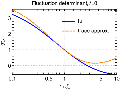
C.4 Growth factor in a spherically-symmetric separate universe

To estimate the dependence of the UV counterterm on the density in Sec. 8.2, we need the linear growth factor for perturbations in the background of a spherical top-hat overdensity. Due to the Birkhoff theorem, such an overdensity can be treated as a separate closed universe. Then the linear growth factor does not depend on the wavenumber of the mode and can be derived by considering spherically symmetric top-hat perturbations.

Consider a spherically symmetric lump of matter with a top-hat profile, whose final density contrast w.r.t. the unperturbed cosmology is equal to $\delta$. Let us additionally perturb this lump by a linear fluctuation $\delta_{L}^{(1)}$. According to the spherical collapse mapping, this fluctuation produces the following perturbation of the non-linear density $\delta^{(1)}$,

$$\delta^{(1)}=\frac{\delta_{L}^{(1)}}{F^{\prime}(\delta_{*})}\;.$$ (C.37)

The density contrast in the separate universe should be normalized to the background density of that universe,

$$\delta_{\rm su}^{(1)}=\frac{\delta^{(1)}}{1+\delta_{*}}\;.$$ (C.38)

This gives for the growth factor in the separate universe:

$$D(\delta_{*},z)=\frac{g(z)}{F^{\prime}(\delta_{*})(1+\delta_{*})}\;.$$ (C.39)

Note that the dependence of the growth factor on redshift and density factorize.

Appendix D Determinant of a matrix made of two vectors

In this Appendix we derive the following formula:

$$\det(\delta_{ij}+a_{i}b_{j}+b_{i}a_{j})=1+2(a\cdot b)+(a\cdot b)^{2}-a^{2}\,b^{2}\;,$$ (D.1)

where dot stands for the scalar product, $a\cdot b=\sum_{i}a_{i}b_{i}$, etc. We start with the trace representation of the determinant,

$$\begin{split}\det(\delta_{ij}+a_{i}b_{j}+b_{i}a_{j})&=\exp\big{[}{\rm Tr}\mathop{\rm ln}\nolimits(\delta_{ij}+a_{i}b_{j}+b_{i}a_{j})\big{]}\\ &=\exp\bigg{[}\sum_{n=1}^{\infty}\frac{(-1)^{n-1}}{n}{\rm Tr}\Big{(}(a_{i}b_{j}+b_{i}a_{j})^{n}\Big{)}\bigg{]}.\end{split}$$ (D.2)

Next, we write an Ansatz,

$$(a_{i}b_{j}+b_{i}a_{j})^{n}=U_{n}a_{i}a_{j}+V_{n}b_{i}b_{j}+W_{n}(a_{i}b_{j}+b_{i}a_{j})\;,$$ (D.3)

where the coefficients obey the recursion relations,

$$U_{n+1}=U_{n}(a\cdot b)+W_{n}b^{2}\;,$$ (D.4a)

$$V_{n+1}=V_{n}(a\cdot b)+W_{n}a^{2}\;,$$ (D.4b)

$$W_{n+1}=U_{n}a^{2}+W_{n}(a\cdot b)=V_{n}b^{2}+W_{n}(a\cdot b)\;.$$ (D.4c)

The last equality implies,

$$U_{n}=C_{n}a^{2}~{},~{}~{}~{}~{}V_{n}=C_{n}b^{2}$$ (D.5)

and the system (D.4) simplifies,

$$C_{n+1}=C_{n}(a\cdot b)+W_{n}\;,$$ (D.6a)

$$W_{n+1}=C_{n}a^{2}b^{2}+W_{n}(a\cdot b)\;.$$ (D.6b)

These are solved by the Ansatz,

$$\begin{pmatrix}C_{n}\\ W_{n}\end{pmatrix}=\begin{pmatrix}C_{0}\\ W_{0}\end{pmatrix}\;\alpha^{n}\;.$$ (D.7)

Substituting this into (D.6) one obtains two lineraly independent solutions; the general solution is their sum,

$$\begin{pmatrix}C_{n}\\ W_{n}\end{pmatrix}=C_{0}^{+}\begin{pmatrix}1\\ \sqrt{a^{2}b^{2}}\end{pmatrix}\alpha_{+}^{n-1}+C_{0}^{-}\begin{pmatrix}1\\ -\sqrt{a^{2}b^{2}}\end{pmatrix}\alpha_{-}^{n-1}\;,$$ (D.8)

where

$$\alpha_{\pm}=(a\cdot b)\pm\sqrt{a^{2}b^{2}}\;.$$ (D.9)

Imposing the initial conditions $C_{1}=0$, $W_{1}=1$ fixes

$$C_{n}=\frac{1}{2\sqrt{a^{2}b^{2}}}(\alpha_{+}^{n-1}-\alpha_{-}^{n-1})\;,~{}~{}~{}~{}W_{n}=\frac{1}{2}(\alpha_{+}^{n-1}+\alpha_{-}^{n-1})\;.$$ (D.10)

Substituting these expressions into (D.3) and taking the trace we find,

$${\rm Tr}\Big{(}(a_{i}b_{j}+b_{i}a_{j})^{n}\Big{)}=\alpha_{+}^{n}+\alpha_{-}^{n}\;.$$ (D.11)

Finally, inserting it into (D.2) we get,

$$\begin{split}\exp\bigg{[}\sum_{n}\frac{(-1)^{n-1}}{n}(\alpha_{+}^{n}+\alpha_{-}^{n})\bigg{]}&=\exp\big{[}\mathop{\rm ln}\nolimits(1+\alpha_{+})+\mathop{\rm ln}\nolimits(1+\alpha_{-})\big{]}\\ &=\exp\big{[}\mathop{\rm ln}\nolimits\big{(}(1+(a\cdot b))^{2}-a^{2}b^{2}\big{)}\big{]},\end{split}$$ (D.12)

which leads to (D.1).

Appendix E Perturbation equations in $\Lambda$CDM

In the real universe the linear growth factor deviates quite significantly from the scale factor, see the right panel of Fig. 2. Thus, it is desirable to compute the prefactor for the exact cosmological model. In this section we present the generalization of Eqs. (5.7), (5.26) to the case of the $\Lambda$CDM universe.

The departures from the EdS approximation are parametrized by the logarithmic growth factor

$$\tilde{f}(\eta)\equiv\frac{d\mathop{\rm ln}\nolimits g}{d\mathop{\rm ln}\nolimits a}\,,$$ (E.1)

where $g(\eta)$ is the linear growth factor in the $\Lambda$CDM cosmology, and $\eta$ now is defined as

$$\eta\equiv\mathop{\rm ln}\nolimits g\,.$$ (E.2)

Starting from the fluid equations for the $\Lambda$CDM universe and proceeding as in Sec. 5.1 one obtains the set of equations for linearized fluctuations with angular number $\ell$ on the spherical collapse solution:

$$\dot{\delta}_{\ell}-\Theta_{\ell}-\partial_{r}\hat{\Psi}\,\partial_{r}\delta_{\ell}-\hat{\Theta}\,\delta_{\ell}-\partial_{r}\hat{\delta}\,\partial_{r}\Psi_{\ell}-\hat{\delta}\,\Theta_{\ell}=0\;,$$ (E.3a)

$$\dot{\Theta}_{\ell}+\left(\frac{3\Omega_{m,\eta}}{2\tilde{f}^{2}}-1\right)\Theta_{\ell}-\frac{3\Omega_{m,\eta}}{2\tilde{f}^{2}}\delta_{\ell}-\partial_{r}\hat{\Psi}\,\partial_{r}\Theta_{\ell}-\partial_{r}\hat{\Theta}\,\partial_{r}\Psi_{\ell}-2\partial_{r}^{2}\hat{\Psi}\,\Theta_{\ell}$$

$$\qquad\qquad\qquad+2\bigg{(}\partial_{r}^{2}\hat{\Psi}-\frac{\partial_{r}\hat{\Psi}}{r}\bigg{)}\,\bigg{(}\frac{2}{r}\partial_{r}\Psi_{\ell}-\frac{\ell(\ell+1)}{r^{2}}\Psi_{\ell}\bigg{)}=0\;,$$ (E.3b)

$$\partial_{r}^{2}\Psi_{\ell}+\frac{2}{r}\partial_{r}\Psi_{\ell}-\frac{\ell(\ell+1)}{r^{2}}\Psi_{\ell}=\Theta_{\ell}\;,$$ (E.3c)

where

$$\Omega_{m,\eta}\equiv\frac{\Omega_{m}}{\Omega_{m}+\Omega_{\Lambda}a^{3}(\eta)}$$ (E.4)

is the time-dependent matter density fraction and the relations between $\Psi$, $\Theta$ and the fluid velocity is now modified,

$$\partial_{i}\Psi=-\frac{u_{i}}{\tilde{f}{\cal H}}\;,\qquad\Theta=-\frac{\partial_{i}u_{i}}{\tilde{f}{\cal H}}\;.$$ (E.5)

Equations (E.3) differ from the EdS case only in the second and third terms in (E.3). The departures are captured by the fraction $\Omega_{m,\eta}/\tilde{f}^{2}$, which is displayed in Fig. 19. One observes that this fraction is quite close to 1 (its value in the EdS universe) until a very recent epoch.

Figure 19: The ratio $\Omega_{m,\eta}/\tilde{f}^{2}$ as a function of $\eta=\mathop{\rm ln}\nolimits g$.

Proceeding along the lines of Sec. 5.2 it is straightforward to derive the equations that replace (5.26) in the $\Lambda$CDM case,

$$\dot{\mu}^{(2)}+\dot{r}_{\eta}^{(2)}\hat{r}_{\eta}^{2}\big{(}1+\hat{\delta}(\hat{r}_{\eta})\big{)}+r_{\eta}^{(2)}\frac{d}{d\eta}\Big{(}\hat{r}_{\eta}^{2}\big{(}1+\hat{\delta}(\hat{r}_{\eta})\big{)}\Big{)}=\hat{r}_{\eta}^{2}\Upsilon_{\delta}(\hat{r}_{\eta})\;,$$ (E.6a)

$$\ddot{r}^{(2)}_{\eta}+\left(\frac{3\Omega_{m,\eta}}{2\tilde{f}^{2}}-1\right)\dot{r}^{(2)}_{\eta}+\frac{\Omega_{m,\eta}}{\tilde{f}^{2}}\bigg{(}1+\frac{3}{2}\hat{\delta}(\hat{r}_{\eta})-\frac{\hat{R}_{*}^{3}}{\hat{r}_{\eta}^{3}}\bigg{)}r^{(2)}_{\eta}+\frac{3\Omega_{m,\eta}}{2\tilde{f}^{2}\hat{r}_{\eta}^{2}}\mu^{(2)}=-\Upsilon_{\Theta}(\hat{r}_{\eta})\;.$$ (E.6b)

Again, the only difference from the EdS equations is the presence of factors $\Omega_{m,\eta}/\tilde{f}^{2}$.

We have computed the aspherical prefactor for the exact reference cosmological model using Eqs. (E.3), (E.6) and found that its deviation from the EdS approximation remains at sub-per cent level.

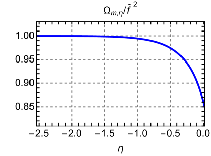
Appendix F Regularization of the WKB integral

F.1 Boundary term in the WKB integral

Here we derive Eq. (7.23). The linear relation (7.19) implies that it is sufficient to prove the corresponding formulae for the $\varkappa$-integrals of the sources $\Upsilon(\hat{r}_{\eta})$. To be concrete, let us focus on the source $\Upsilon_{\delta}$, the reasoning for $\Upsilon_{\Theta}$ is the same. We start with the asymptotic expression for the Bessel function in the vicinity of the turning point, Eq. (10.19.8) from [60],

$$J_{\nu}(\nu+a\nu^{1/3})=\frac{2^{1/3}}{\nu^{1/3}}{\rm Ai}(-2^{1/3}a)+O(1/\nu)\;,$$ (F.1)

where ${\rm Ai(z)}$ is the Airy function. Comparing it with (5.9) and recalling the definition of spherical Bessel functions (A.12) we find the initial conditions for the perturbations at $\eta\to-\infty$ in the vicinity of the point $\varkappa r=1$,

$$\delta_{\ell}=\Theta_{\ell}=\frac{{\rm e}^{\eta}}{(\ell+1/2)^{5/6}}\cdot(2\pi)^{3/2}2^{1/3}{\rm Ai}\big{[}-2^{1/3}(\ell+1/2)^{2/3}(\varkappa r-1)\big{]}\;,$$ (F.2a)

$$\Psi_{l}=-\frac{{\rm e}^{\eta}}{(\ell+1/2)^{17/6}}\cdot\frac{(2\pi)^{3/2}2^{1/3}}{\varkappa^{2}}{\rm Ai}\big{[}-2^{1/3}(\ell+1/2)^{2/3}(\varkappa r-1)\big{]}\;.$$ (F.2b)

From these expressions we infer the scaling of the fields and their derivatives at all moments of time,

$$\delta_{\ell},\Theta_{\ell}=O(\ell^{-5/6})~{},~{}~{}~{}~{}\Psi_{\ell}=O(\ell^{-17/6})~{},~{}~{}~{}~{}\partial_{r}\Psi_{\ell}=O(\ell^{-13/6})~{},~{}~{}~{}~{}\partial^{2}_{r}\Psi_{\ell}=O(\ell^{-3/2})\;.$$ (F.3)

This implies that the terms with derivatives in the Poisson equation (5.7c) are subdominant compared to the last term on the l.h.s., so that the relation between $\Psi_{\ell}$ and $\Theta_{\ell}$ becomes very simple,

$$\Psi_{\ell}=-\frac{r^{2}}{(\ell+1/2)^{2}}\Theta_{\ell}\;.$$ (F.4)

Inspecting the magnitude of various terms in Eqs. (5.7a), (5.7) we find that they also simplify,

$$\frac{d\delta_{\ell}}{d\eta}\bigg{|}_{\rm flow}-\hat{\Theta}\delta_{\ell}-(1+\hat{\delta})\Theta_{\ell}=0\;,$$ (F.5a)

$$\frac{d\Theta_{\ell}}{d\eta}\bigg{|}_{\rm flow}-\frac{3}{2}\delta_{\ell}+\bigg{(}\frac{1}{2}-2\frac{\partial_{r}\hat{\Psi}}{r}\bigg{)}\Theta_{\ell}=0\;.$$ (F.5b)

Similarly to Eqs. (7.8) they have the ultralocal form (no $r$-derivatives of the perturbations), so that the fields evolve independently along different flow lines. Besides, in the small vicinity of the ‘turning flow line’ $R=1/\varkappa$ the background functions can be considered as $r$-independent. Thus, in the comoving frame the time-evolution of the perturbations factorizes from their spatial dependence, and we obtain,

$$\delta_{\ell}=\frac{\alpha(\eta)}{(\ell+1/2)^{5/6}}\cdot(2\pi)^{3/2}2^{1/3}{\rm Ai}\big{[}-2^{1/3}(\ell+1/2)^{2/3}(\varkappa R-1)\big{]};,$$ (F.6a)

$$\Theta_{\ell}=\frac{\beta(\eta)}{(\ell+1/2)^{5/6}}\cdot(2\pi)^{3/2}2^{1/3}{\rm Ai}\big{[}-2^{1/3}(\ell+1/2)^{2/3}(\varkappa R-1)\big{]};,$$ (F.6b)

$$\Psi_{\ell}=\frac{\gamma(\eta)}{(\ell+1/2)^{17/6}}\cdot\frac{(2\pi)^{3/2}2^{1/3}}{\varkappa^{2}}{\rm Ai}\big{[}-2^{1/3}(\ell+1/2)^{2/3}(\varkappa R-1)\big{]}\;,$$ (F.6c)

where $\alpha,\beta,\gamma$ are some functions whose precise form is not important to us.

Let us evaluate the following integral:

$$\begin{split}&\int_{\frac{1-\epsilon}{R_{*}}}^{\frac{1+\epsilon}{R_{*}}}d\varkappa\,\varphi(\varkappa)\Upsilon_{\delta}(\hat{r}_{\eta},\eta;\varkappa)=-\frac{1}{4\pi}\frac{\alpha(\eta)\gamma(\eta)}{(\ell+1/2)^{3}}\cdot 2(2\pi)^{3}\frac{\partial R}{\partial r}\bigg{|}_{\hat{r}_{\eta}}\\ &\times\int_{\frac{1-\epsilon}{R_{*}}}^{\frac{1+\epsilon}{R_{*}}}d\varkappa\frac{\varphi(\varkappa)}{\varkappa}{\rm Ai}\big{[}-2^{1/3}(\ell+1/2)^{2/3}(\varkappa R_{*}-1)\big{]}{\rm Ai}^{\prime}\big{[}-2^{1/3}(\ell+1/2)^{2/3}(\varkappa R_{*}-1)\big{]}\\ &=\frac{1}{8\pi}\frac{\alpha(\eta)\gamma(\eta)}{(\ell+1/2)^{11/3}}\cdot 2^{2/3}(2\pi)^{3}\frac{\partial R}{\partial r}\bigg{|}_{\hat{r}_{\eta}}\varphi(1/R_{*})\Big{[}{\rm Ai}\big{(}-2^{1/3}(\ell+1/2)^{2/3}\epsilon\big{)}\Big{]}^{2}\\ &=\frac{1}{8\pi}\frac{\partial R}{\partial r}\bigg{|}_{\hat{r}_{\eta}}\frac{\varphi(1/R_{*})}{R_{*}^{2}}\;\delta_{\ell}\,\Psi_{\ell}\Big{|}_{\hat{r}_{\eta},\,\varkappa=(1+\epsilon)/R_{*}}\;,\end{split}$$ (F.7)

where we have substituted Eq. (5.14a) and in passing to the third line used that the Airy function is exponentially suppressed at positive values of its argument. At $\ell^{-2/3}\ll\epsilon\ll 1$ we can use the WKB form (7.4) for $\delta_{\ell}$ and $\Psi_{\ell}$. Substituting it into the last expression in (F.7) and averaging away the oscillating pieces we obtain,

$$\int_{(1-\epsilon)/R_{*}}^{(1+\epsilon)/R_{*}}d\varkappa\,\varphi(\varkappa)\Upsilon_{\delta}(\hat{r}_{\eta},\eta;\varkappa)=\frac{1}{4\pi k^{2}}\frac{\varphi(1/R_{*})}{R_{*}^{2}}\frac{\partial R}{\partial r}\bigg{|}_{\hat{r}_{\eta}}\;\tilde{\delta}_{\ell 1}\tilde{\Psi}_{\ell 1}\Big{|}_{\hat{r}_{\eta},\,\varkappa=(1+\epsilon)/R_{*}}\;.$$ (F.8)

Using the initial conditions (7.12b), (7.12c) and the ultralocality of the evolution in the vicinity of the turning point it is straightforward to show that

$$\tilde{\delta}_{\ell 1}\tilde{\Psi}_{\ell 1}\Big{|}_{\hat{r}_{\eta},\;\varkappa=(1+\epsilon)/R_{*}}=-\frac{4R_{*}}{\sqrt{\epsilon}}\lim_{\epsilon^{\prime}\to 0}(\epsilon^{\prime})^{3/2}\tilde{\delta}_{\ell 1}\frac{\partial\tilde{\Psi}_{\ell 1}}{\partial R}\Big{|}_{\hat{r}_{\eta},\;\varkappa=(1+\epsilon^{\prime})/R_{*}}\;,$$ (F.9a)

$$(\tilde{\delta}_{\ell 1}\tilde{\Psi}_{\ell 2}-\tilde{\delta}_{\ell 2}\tilde{\Psi}_{\ell 1})\Big{|}_{\hat{r}_{\eta},\;\varkappa=(1+\epsilon)/R_{*}}=O(\epsilon^{-1})\;.$$ (F.9b)

The latter combination appears in $\Upsilon_{\delta}$ multiplied by $\frac{\partial S_{\ell}}{\partial R}$, see Eq. (7.18a). Taking into account the expression

$$\frac{\partial S_{\ell}}{\partial R}=\frac{\sqrt{(\varkappa R)^{2}-1}}{\varkappa R}=O(\sqrt{\epsilon})\;,$$ (F.10)

one concludes that the corresponding term does not contribute into $\lim_{\epsilon\to 0}\epsilon^{3/2}\Upsilon_{\delta}$. Then Eq. (F.8) can be cast into the form,

$$\int_{(1-\epsilon)/R_{*}}^{(1+\epsilon)/R_{*}}d\varkappa\,\varphi(\varkappa)\Upsilon_{\delta}(\hat{r}_{\eta},\eta;\varkappa)=-\frac{2\varphi(1/R_{*})}{R_{*}\sqrt{\epsilon}}\lim_{\epsilon^{\prime}\to 0}(\epsilon^{\prime})^{3/2}\Upsilon_{\delta}\big{(}\hat{r}_{\eta},\eta;\varkappa=(1+\epsilon^{\prime})/R_{*}\big{)}\;.$$ (F.11)

This proves the expression of the type (7.23) for the integrals involving $\Upsilon_{\delta}$. The argument for the integrals involving $\Upsilon_{\Theta}$ is completely analogous. This completes the derivation of Eq. (7.23).

F.2 Evaluation of the $\varkappa$-integral

Numerical evaluation of the WKB integral (7.23) presents a non-trivial challenge. Indeed, in the limit $\epsilon\to 0$ the expression on the r.h.s. contains a difference between two large numbers that must be evaluated with very high accuracy, which may be impractical. On the other hand, at finite values of $\epsilon$ the error is estimated as $O(\sqrt{\epsilon})$. Thus, to reach an acceptable level of accuracy of, say, $1\%$ one would have to go down to $\epsilon\sim 10^{-4}$. To improve the convergence of the numerical procedure, we derive here an expression that explicitly takes into account the $O(\sqrt{\epsilon})$ corrections.

Let us introduce dimensionless variables,

$$x=\varkappa R_{*}-1~{},~{}~{}~{}~{}~{}y=R/R_{*}-1\;.$$ (F.12)

At small $x$ we have

$$q(x)=q_{3\over 2}\,x^{-3/2}+q_{1\over 2}\,x^{-1/2}+O(\sqrt{x})~{},~{}~{}~{}~{}~{}\varphi(x)=\varphi_{0}+\varphi_{1}\,x+O(x^{2})\;,$$ (F.13)

And the integral takes the form,

$$\mathchoice{{\vbox{\hbox{$\textstyle-$}}\kern-4.86108pt}}{{\vbox{\hbox{$\scriptstyle-$}}\kern-3.25pt}}{{\vbox{\hbox{$\scriptscriptstyle-$}}\kern-2.29166pt}}{{\vbox{\hbox{$\scriptscriptstyle-$}}\kern-1.875pt}}\!\int d\varkappa\,q(\varkappa)\varphi(\varkappa)=\frac{1}{R_{*}}\bigg{[}-\frac{2q_{3\over 2}\varphi_{0}}{\sqrt{\epsilon}}+2(q_{3\over 2}\varphi_{1}+q_{1\over 2}\varphi_{0})\sqrt{\epsilon}+\int_{\epsilon}^{\infty}dx\,q(x)\varphi(x)+O(\epsilon^{3/2})\bigg{]}\;.$$ (F.14)

We expand the sources $\Upsilon_{i}$, $i=\delta,\Theta$ in a similar way,

$$\Upsilon_{i}(\hat{r}_{\eta})=\frac{1}{k^{2}(\ell+1/2)^{2}}\big{(}\Upsilon_{i,{3\over 2}}\,x^{-3/2}+\Upsilon_{i,{1\over 2}}\,x^{-1/2}+O(\sqrt{x})\big{)}\;.$$ (F.15)

Substituting this into (7.19) and comparing with (7.20) we find,

$$q_{3\over 2}=\int_{-\infty}^{0}d\eta\;\big{(}K_{\delta}(\eta)\Upsilon_{\delta,{3\over 2}}(\eta)+K_{\Theta}(\eta)\Upsilon_{\Theta,{3\over 2}}(\eta)\big{)}\;,$$ (F.16a)

$$q_{1\over 2}=\int_{-\infty}^{0}d\eta\;\big{(}K_{\delta}(\eta)\Upsilon_{\delta,{1\over 2}}(\eta)+K_{\Theta}(\eta)\Upsilon_{\Theta,{1\over 2}}(\eta)\big{)}\;.$$ (F.16b)

Here the kernels $K_{i}$ as well as the sources $\Upsilon_{i,{3\over 2}}$, $\Upsilon_{i,{1\over 2}}$ are regular functions of time (and are independent of $x$), so that $q_{3\over 2}$, $q_{1\over 2}$ can be obtained by a straightforward numerical integration of eqs. (5.26) with the corresponding sources. Our task is to derive expressions for $\Upsilon_{i,{3\over 2}}$, $\Upsilon_{i,{1\over 2}}$.

For $y\ll x\ll 1$ we write,

$$\tilde{\delta}_{\ell 1}(\eta,y;x)=\big{(}\alpha_{0}(\eta)+\alpha_{1}(\eta)x+\alpha_{2}(\eta)y+O(x^{2},xy)\big{)}\,\tilde{\delta}_{\ell 1}^{\rm sing}(y;x)\;,$$ (F.17a)

$$\tilde{\Theta}_{\ell 1}(\eta,y;x)=\big{(}\beta_{0}(\eta)+\beta_{1}(\eta)x+\beta_{2}(\eta)y+O(x^{2},xy)\big{)}\,\tilde{\delta}_{\ell 1}^{\rm sing}(y;x)\;.$$ (F.17b)

where

$$\begin{split}\tilde{\delta}_{\ell 1}^{\rm sing}(y;x)&\equiv\frac{2\pi}{(\ell+1/2)}\cdot\frac{1}{\sqrt{\varkappa R}\,[(\varkappa R)^{2}-1]^{1/4}}\\ &=\frac{2\pi}{(\ell+1/2)}\cdot\frac{1}{2^{1/4}x^{1/4}}\bigg{[}1-\frac{5}{8}x-y\bigg{(}\frac{1}{4x}+\frac{23}{32}\bigg{)}\bigg{]}\;.\end{split}$$ (F.18)

In the last expression we expanded to the first subleading order in $x$ and kept only up to linear order in $y$. This is sufficient for our purposes as we will only need the values of the fields and their first derivatives at $y=0$. The functions $\alpha_{0}(\eta)$ etc. can be found by integrating Eqs. (7.8) in the vicinity of the point $x=y=0$ with smooth $x$- and $y$-independent initial conditions $\tilde{\delta}_{\ell 1},\tilde{\Theta}_{\ell 1}={\rm e}^{\eta}$ at $\eta\to-\infty$. From (F.17) one reads off the values of the fields at $y=0$,

$$\tilde{\delta}_{\ell 1}(\eta,0;x)=\frac{2\pi}{(\ell+1/2)}\cdot\frac{1}{2^{1/4}x^{1/4}}\bigg{[}\alpha_{0}+x\,\bigg{(}-\frac{5}{8}\alpha_{0}+\alpha_{1}\bigg{)}\bigg{]}\;,$$ (F.19a)

$$\tilde{\Theta}_{\ell 1}(\eta,0;x)=\frac{2\pi}{(\ell+1/2)}\cdot\frac{1}{2^{1/4}x^{1/4}}\bigg{[}\beta_{0}+x\,\bigg{(}-\frac{5}{8}\beta_{0}+\beta_{1}\bigg{)}\bigg{]}\;.$$ (F.19b)

Next, we have,

$$\frac{\partial S_{\ell}}{\partial r}\Big{|}_{y=0}=\frac{\partial R}{\partial r}\Big{|}_{\hat{r}_{\eta}}\cdot\sqrt{2x}+O(x^{3/2})\;,~{}~{}~{}~{}\frac{\partial^{2}S_{\ell}}{\partial r^{2}}\Big{|}_{y=0}=\frac{1}{R_{*}}\cdot\bigg{(}\frac{\partial R}{\partial r}\bigg{)}^{2}\Big{|}_{\hat{r}_{\eta}}\cdot\frac{1}{\sqrt{2x}}+O(x^{1/2})\;.$$ (F.20)

Substituting this into (7.5a) we obtain,

$$\tilde{\Psi}_{\ell 1}\Big{|}_{y=0}= -\frac{2\pi\hat{r}^{2}_{\eta}}{(\ell+1/2)R_{*}^{2}}\cdot\frac{1}{2^{1/4}x^{1/4}}\bigg{[}\beta_{0}+x\,\bigg{(}\frac{11\beta_{0}}{8}-2\beta_{0}\bigg{(}\frac{\partial\mathop{\rm ln}\nolimits r_{in}}{\partial\mathop{\rm ln}\nolimits r}\bigg{)}^{2}+\beta_{1}\bigg{)}\bigg{]}\;,$$ (F.21a)

$$\tilde{\Psi}_{\ell 1}^{\prime}\Big{|}_{y=0}= -\frac{2\pi\hat{r}^{2}_{\eta}}{(\ell+1/2)R_{*}^{3}}\frac{\partial R}{\partial r}\cdot\frac{1}{2^{1/4}x^{5/4}}\bigg{[}-\frac{\beta_{0}}{4}$$

$$\qquad+x\,\bigg{(}-\frac{39}{32}\beta_{0}-\frac{3\beta_{0}}{2}\bigg{(}\frac{\partial\mathop{\rm ln}\nolimits R}{\partial\mathop{\rm ln}\nolimits r}\bigg{)}^{2}+2\beta_{0}\bigg{(}\frac{\partial\mathop{\rm ln}\nolimits R}{\partial\mathop{\rm ln}\nolimits r}\bigg{)}^{-1}-\frac{\beta_{1}}{4}+\beta_{2}\bigg{)}\bigg{]}\;.$$ (F.21b)

We now show that the second-order WKB perturbations do not contribute at the order we are interested in. First, we demonstrate that the r.h.s. of Eqs. (7.9) evaluated at $y=0$ is of order $O(x^{1/4})$. Indeed, using (F.20), (F.21a) we find for Eq. (7.9a),

$$S_{\ell}^{\prime}\Psi_{\ell 1}\Big{|}_{y=0}\sim\sqrt{x}\cdot x^{-1/4}\sim x^{1/4}\;.$$ (F.22)

On the r.h.s. of (7.9b) the only term that can potentially be of order $O(x^{-3/4})$ has the form,

$$-\frac{4S_{\ell}^{\prime}\tilde{\Psi}_{\ell 1}^{\prime}+2S_{l}^{\prime\prime}\tilde{\Psi}_{\ell 1}}{1+(\varkappa rS_{\ell}^{\prime})^{2}}\bigg{(}\partial^{2}_{r}\hat{\Psi}-\frac{\partial\hat{\Psi}}{r}\bigg{)}\bigg{|}_{y=0}\;.$$ (F.23)

However, from (F.20), (F.21) we find that the divergent terms cancel out, so that

$$(2S_{\ell}^{\prime}\tilde{\Psi}_{\ell 1}^{\prime}+S_{l}^{\prime\prime}\tilde{\Psi}_{\ell 1})\Big{|}_{y=0}=O(x^{1/4})\;.$$ (F.24)

Thus, working only up to order $O(x^{-3/4})$ we can neglect the r.h.s. in Eqs. (7.9) and write,

$$\tilde{\delta}_{\ell 2}(\eta,0;x)=\big{(}\alpha_{0}(\eta)+\alpha_{1}(\eta)x\big{)}\,\tilde{\delta}_{\ell 2}^{\rm sing}(0;x)\;,$$ (F.25a)

$$\tilde{\Theta}_{\ell 2}(\eta,0;x)=\big{(}\beta_{0}(\eta)+\beta_{1}(\eta)x\big{)}\,\tilde{\delta}_{\ell 2}^{\rm sing}(0;x)\;,$$ (F.25b)

where

$$\begin{split}\tilde{\delta}_{\ell 2}^{\rm sing}(0;x)\equiv&\frac{\pi}{4(\ell+1/2)}\cdot\sqrt{\frac{\varkappa}{R_{*}}}\,\bigg{(}\frac{5}{3[(\varkappa R_{*})^{2}-1]^{7/4}}+\frac{1}{[(\varkappa R_{*})^{2}-1]^{3/4}}\bigg{)}\\ =&\frac{\pi}{4(\ell+1/2)R_{*}}\cdot\frac{1}{2^{7/4}x^{7/4}}\bigg{[}\frac{5}{3}+\frac{11}{8}x+O(x^{2})\bigg{]}\;.\end{split}$$ (F.26)

Next, from (7.5b) and using (F.24) we get,

$$\tilde{\Psi}_{\ell 2}\Big{|}_{y=0}=-\frac{\tilde{\Theta}_{\ell 2}}{(S_{\ell}^{\prime})^{2}+(\varkappa r)^{-2}}\Big{|}_{y=0}+O(x^{1/4})\;.$$ (F.27)

Then the term in the source $\Upsilon_{\delta}$ containing second-order WKB perturbations is (see Eq. (7.18a)),

$$S_{\ell}^{\prime}(\tilde{\delta}_{\ell 1}\tilde{\Psi}_{\ell 2}-\tilde{\delta}_{\ell 2}\tilde{\Psi}_{\ell 1})\Big{|}_{y=0}=S_{\ell}^{\prime}\;\frac{-\tilde{\delta}_{\ell 1}\tilde{\Theta}_{\ell 2}+\tilde{\delta}_{\ell 2}\tilde{\Theta}_{\ell 1}}{(S_{\ell}^{\prime})^{2}+(\varkappa r)^{-2}}\bigg{|}_{y=0}+O(\sqrt{x})=O(\sqrt{x})\;,$$ (F.28)

where in the last equality we have used the expressions (F.17), (F.25). Similarly, one shows that the second-order WKB contribution in $\Upsilon_{\Theta}$ is also of order $O(\sqrt{x})$. Given that we are keeping only terms up to order $O(x^{-1/2})$, we conclude that the second-order WKB contributions can be omitted altogether.

It remains to substitute the expressions (F.19), (F.21) into (7.18). A straightforward calculation yields,

$$\Upsilon_{\delta,{3\over 2}}= \frac{\pi\hat{r}^{2}_{\eta}}{2\sqrt{2}R_{*}^{3}}\frac{\partial R}{\partial r}\bigg{|}_{y=0}\alpha_{0}(\eta)\beta_{0}(\eta)\;,$$ (F.29a)

$$\Upsilon_{\Theta,{3\over 2}}= -\frac{\pi\hat{r}^{2}_{\eta}}{2\sqrt{2}R_{*}^{3}}\frac{\partial R}{\partial r}\bigg{|}_{y=0}\beta_{0}^{2}(\eta)\;,$$ (F.29b)

$$\Upsilon_{\delta,{1\over 2}}= \frac{\sqrt{2}\pi\hat{r}^{2}_{\eta}}{R_{*}^{3}}\frac{\partial R}{\partial r}\bigg{|}_{y=0}\bigg{[}\alpha_{0}\beta_{0}\bigg{(}\frac{17}{16}+\frac{3}{2}\bigg{(}\frac{\partial\mathop{\rm ln}\nolimits R}{\partial\mathop{\rm ln}\nolimits r}\bigg{)}^{2}-2\bigg{(}\frac{\partial\mathop{\rm ln}\nolimits R}{\partial\mathop{\rm ln}\nolimits r}\bigg{)}^{-1}\bigg{)}$$

$$\qquad\qquad\qquad\qquad+\frac{1}{4}(\alpha_{0}\beta_{1}+\alpha_{1}\beta_{0})-\alpha_{0}\beta_{2}\bigg{]}\;,$$ (F.29c)

$$\Upsilon_{\Theta,{1\over 2}}= \frac{\sqrt{2}\pi\hat{r}^{2}_{\eta}}{R_{*}^{3}}\frac{\partial R}{\partial r}\bigg{|}_{y=0}\bigg{[}\beta_{0}^{2}\bigg{(}-\frac{17}{16}-\frac{1}{2}\bigg{(}\frac{\partial\mathop{\rm ln}\nolimits R}{\partial\mathop{\rm ln}\nolimits r}\bigg{)}^{2}+\bigg{(}\frac{\partial\mathop{\rm ln}\nolimits R}{\partial\mathop{\rm ln}\nolimits r}\bigg{)}^{-1}\bigg{)}-\frac{\beta_{0}\beta_{1}}{2}+\beta_{0}\beta_{2}\bigg{]}\;.$$ (F.29d)

These are the final expressions for the sources to be used in Eqs. (F.16).

Appendix G Numerical procedure

In this Appendix we discuss the details of our numerical method, which is implemented in the open-source code AsPy [61] written in Python using scipy and numpy libraries.

We first cast the partial differential equations (5.7) in the form suitable for numerical solution using finite differences. In this section we will omit the subscript $\ell$ denoting linear aspherical perturbations. We switch to the Lagrangian coordinate $R$ comoving with the background flow, which allows us to absorb the shift terms into the time derivative,

$$\frac{\partial}{\partial\eta}-\partial_{r}\hat{\Psi}\frac{\partial}{\partial r}\equiv\frac{d}{d\eta}\bigg{|}_{\text{flow}}\,.$$ (G.1)

Equations (5.7a), (5.7) take the form,

$$\frac{d\delta}{d\eta}=A_{1}(\eta,R)\delta+A_{2}(\eta,R)\Theta+A_{3}(\eta,R)\partial_{R}\Psi\,,$$ (G.2a)

$$\frac{d\Theta}{d\eta}=\frac{3}{2}\delta+A_{4}(\eta,R)\Theta+A_{5}(\eta,R)\partial_{R}\Psi+\ell(\ell+1)A_{6}(\eta,R)\Psi\,,$$ (G.2b)

where we defined the following background functions:

$$A_{1}=\hat{\Theta}\,, A_{4}=-\frac{1}{2}+2\left(\hat{\Theta}-\frac{2}{r}\partial_{r}\hat{\Psi}\right)\,,$$ (G.3a)

$$A_{2}=1+\hat{\delta}\,, A_{5}=\frac{1}{\frac{\partial r}{\partial R}}\left(\frac{1}{\frac{\partial r}{\partial R}}\partial_{R}\hat{\Theta}-\frac{4}{r}\left(\hat{\Theta}-3\frac{\partial_{r}\hat{\Psi}}{r}\right)\right)\,,$$ (G.3b)

$$A_{3}=\frac{1}{\left(\frac{\partial r}{\partial R}\right)^{2}}\partial_{R}\hat{\delta}\,, A_{6}=2\left(\hat{\Theta}-3\frac{\partial_{r}\hat{\Psi}}{r}\right)\frac{1}{r^{2}}\,.$$ (G.3c)

The initial conditions for the density and velocity fields are given by Eqs. (5.9a). Note that Eqs. (G.2) do not contain spatial derivatives of $\delta$ or $\Theta$, so we do not need to impose any boundary conditions on them.

The Euler and continuity equations are supplemented by the Poisson equation

$$\left(\partial^{2}_{r}+\frac{2\partial_{r}}{r}-\frac{\ell(\ell+1)}{r^{2}}\right)\Psi(\eta,R)=\Theta(\eta,R)\,.$$ (G.4)

The boundary conditions for the velocity potential are given by,

$$\begin{split}&\Psi(\eta,R)\propto r^{\ell}(R)\,,\quad\text{at}\quad R\to 0\\ &\Psi(\eta,R_{max})={\rm e}^{(\eta-\eta_{min})}\Psi(\eta_{min},R_{max})\,.\end{split}$$ (G.5)

The boundary condition at the origin is dictated by the structure of the Poisson equation (5.7c). The second condition comes from the assumption that at spatial infinity the velocity potential follows the linear evolution, which is justified since the background profile falls off quickly outside the window function.

We work on an equally-spaced rectangular lattice with $N_{R}\times N_{\eta}$ nodes and physical size $[R_{min},R_{max}]\times[\eta_{min},0]$. We implement an implicit second-order Runge-Kutta scheme (RK2) for the Euler and continuity equations. For the Poisson equation we use an implicit second-order finite difference scheme.

We use the discrete version of the fluctuation operator obtained by rewriting the integrals in the exponent of (2.38) in a discrete form and taking the corresponding Gaussian integral. This yields,

$$\mathcal{O}_{\ell}=\delta_{ij}+2\hat{\lambda}\frac{\Delta k}{(2\pi)^{3}}k_{i}k_{j}Q_{\ell}(k_{i},k_{j})\sqrt{P(k_{i})P(k_{j})}\,,$$ (G.6)

with $i,j=0,\ldots,N$; $\Delta k=(k_{N}-k_{0})/N$. One can check that this definition gives the correct continuous limit for the trace:

$$\sum_{i=0}^{N}\frac{\Delta kk^{2}_{i}}{(2\pi)^{3}}\,Q_{\ell}(k_{i},k_{i})P(k_{i})\xrightarrow{N\to\infty}\int_{0}^{\infty}[dk]\,Q_{\ell}(k,k)P(k)={\rm Tr}\,Q_{\ell}P\;.$$ (G.7)

We implement the algorithm for computing the aspherical determinant from Sec. 5.3. At the first step the code computes the background functions (G.3) required for solving the fluid equations on the grid. To this end we make a sample of $\sim 20$ values of $\delta_{*}$ in the range $[-0.9,9]$ and use the spherical collapse linear profile (2.27) to compute the non-linear background configuration defined by the equations from Sec. C.1.

At the second step we sample the momentum space and compute the evolution of linear fluctuations given by the finite difference approximation to the equations (G.2), (G.4) with appropriate initial and boundary conditions for each momentum $k_{i}$ from the sample. We use the sample of $N=200$ wavenumbers which we found sufficient for our purposes.

We found that the following grid parameters lead to a good convergence for most of the multipoles in the $\delta_{*}$-range of interest:

$$\begin{split}&R_{min}=10^{-2}\,\text{Mpc}/h\,,\quad R_{max}=10\cdot R_{*}\,,\quad N_{R}=1000\,,\\ &\eta_{min}=-7\,,\quad N_{\eta}=500\,.\end{split}$$ (G.8)

For the dipole we increased the spatial extent of the grid to $R_{max}=15\cdot R_{*}$, $N_{R}=1500$. We have run several tests and found that increasing the grid resolution further or moving the box boundaries can only change the final results at the $0.1\%$ level.

At the third step we use the linear mode functions computed in step 2 to construct the sources $\Upsilon_{\Theta,\delta}$ for all different pairs of momenta $(k_{i},k_{j})$, $i,j=0,\dots,N$. For the dipole sector, we also construct the sources $B_{\Theta,\delta}$

At the fourth step we solve the finite difference equations for the time evolution of $\mu^{(2)}$ and $r^{(2)}_{\eta}$ obtained by discretizing Eqs. (5.26). This yields the matrix $Q_{\ell}(k_{i},k_{j})$, which is used to obtain the desired determinant. In the dipole sector we separately compute $\breve{Q}_{\ell}(k_{i},k_{j})$, $B(k_{i})$, and $A$ using (5.26) with the corresponding sources (6.12). The final determinant is obtained upon multiplying the IR-sensitive determinant $\mathcal{D}_{IR}$ and the IR-safe determinant $\det(\mathbb{1}+2\hat{\lambda}\sqrt{P}\breve{Q}_{\ell}\sqrt{P})$. As a cross-check, we computed $A$ both by solving Eqs. (5.26) and from the relation (6.24), which yielded results that agree at the per mil level.

We have validated our code by computing the determinant of the monopole fluctuations and comparing it to the analytic expression (C.34). The results of this test are displayed in Fig. 20. Numerical procedure agrees with the analytic formula at per mil level.

Figure 20: The fluctuation determinant in the monopole sector: the result of our numerical procedure (dots) vs. Eq. (C.34) (line).

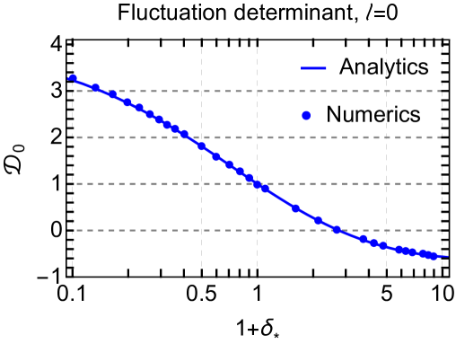
Appendix H A comment on log-normal model

It has long been known that the observed counts-in-cells distribution can be well approximated by log-normal [24, 25, 26, 27],

$$\mathcal{P}_{\text{log-normal}}(\delta_{*})=\frac{1}{\sqrt{2\pi\sigma^{2}_{\rm ln}}(1+\delta_{*})}\exp\left\{-\frac{\big{(}\mathop{\rm ln}\nolimits(1+\delta_{*})+\sigma^{2}_{\rm ln}/2\big{)}^{2}}{2\sigma^{2}_{\rm ln}}\right\}\,,$$ (H.1)

where $\sigma_{\rm ln}^{2}=\langle[\mathop{\rm ln}\nolimits(1+\delta_{*})]^{2}\rangle$ is the log-density variance, to be fitted from the data. The mean of the distribution (H.1) is adjusted to ensure $\langle\delta_{*}\rangle=0$. The success of this model is partially due to the fact that the spherical collapse mapping $F(\delta_{*})$ is close to $\mathop{\rm ln}\nolimits(1+\delta_{*})$ for moderate density contrasts, see the left panel of Fig. 21. The difference grows for bigger $|\delta_{*}|$, but, curiously enough, gets largely compensated by the scale dependence of $\sigma_{R_{*}}$. This compensation is a mere coincidence due to the shape of the power spectrum at mildly non-linear scales [29, 30]. Indeed, consider, for example, a universe with a power-law power spectrum $P(k)\propto k^{n}$. In such a universe the variance scales as $\sigma_{R_{*}}^{2}\propto(1+\delta_{*})^{-1-n/3}$, which clearly depends on the slope $n$. On the other hand, spherical collapse mapping is determined exclusively by dynamics and is insensitive to the statistics of the initial conditions. One concludes that changing the slope of the power spectrum would destroy the consipracy and the log-normal model would fail.

Figure 21: Left panel: The functions defining the leading exponential behavior of the log-normal PDF (H.1) and our theoretical PDF (2.30). The log-variance $\sigma_{\rm ln}$ is found from the fit to N-body data. Right panel: Residuals of the N-body data with respect to the best fit log-normal models at different redshifts. $\sigma_{\rm ln}$ is refitted for each $z$ independently. The cell radius is $r_{*}=10\,\text{Mpc}/h$.

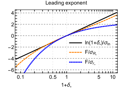
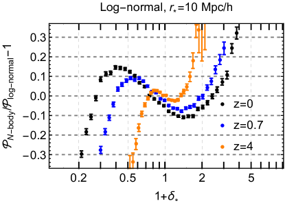
Although the log-normal PDF gives a good leading order approximation, it does not incorporate the correct prefactor. As a consequence, it is unable to describe the data with the accuracy better than $\sim 10\%$ even at moderate densities and quickly deviates from the data in the tails [42, 31]. This is illustrated in the right panel of Fig. 21 where we show the residuals of the N-body data with respect to the best fit log-normal model.

The agreement between the log-normal model and the data can be improved by artificially allowing the minimal value of $\delta_{*}$ to be different from $-1$. This was observed e.g. for the case of the projected density and convergence fields in Refs. [65, 66]. However, allowing $\delta_{*,min}$ to be different from $-1$ appears hard to justify on the physical grounds.

References

- [1] A. Schneider et al., JCAP 1604, no. 04, 047 (2016) [arXiv:1503.05920 [astro-ph.CO]].
- [2] F. Bernardeau, S. Colombi, E. Gaztanaga and R. Scoccimarro, Phys. Rept. 367, 1 (2002) [astro-ph/0112551].
- [3] R. Scoccimarro and J. Frieman, Astrophys. J. Suppl. 105, 37 (1996) [astro-ph/9509047].
- [4] A. Kehagias and A. Riotto, Nucl. Phys. B 873, 514 (2013) [arXiv:1302.0130 [astro-ph.CO]].
- [5] M. Peloso and M. Pietroni, JCAP 1305, 031 (2013) [arXiv:1302.0223 [astro-ph.CO]].
- [6] D. Blas, M. Garny and T. Konstandin, JCAP 1309, 024 (2013) [arXiv:1304.1546 [astro-ph.CO]].
- [7] P. Creminelli, J. Norena, M. Simonovic and F. Vernizzi, JCAP 1312, 025 (2013) [arXiv:1309.3557 [astro-ph.CO]].
- [8] B. Horn, L. Hui and X. Xiao, JCAP 1409, no. 09, 044 (2014) [arXiv:1406.0842 [hep-th]].
- [9] D. Blas, M. Garny, M. M. Ivanov and S. Sibiryakov, JCAP 1607, no. 07, 052 (2016) [arXiv:1512.05807 [astro-ph.CO]].
- [10] L. Senatore and M. Zaldarriaga, JCAP 1502, no. 02, 013 (2015) [arXiv:1404.5954 [astro-ph.CO]].
- [11] T. Baldauf, M. Mirbabayi, M. Simonovic and M. Zaldarriaga, Phys. Rev. D 92, no. 4, 043514 (2015) [arXiv:1504.04366 [astro-ph.CO]].
- [12] D. Blas, M. Garny, M. M. Ivanov and S. Sibiryakov, JCAP 1607, no. 07, 028 (2016) [arXiv:1605.02149 [astro-ph.CO]].
- [13] M. M. Ivanov and S. Sibiryakov, JCAP 1807, no. 07, 053 (2018) [arXiv:1804.05080 [astro-ph.CO]].
- [14] D. Baumann, A. Nicolis, L. Senatore and M. Zaldarriaga, JCAP 1207, 051 (2012) [arXiv:1004.2488 [astro-ph.CO]].
- [15] J. J. M. Carrasco, M. P. Hertzberg and L. Senatore, JHEP 1209, 082 (2012) [arXiv:1206.2926 [astro-ph.CO]].
- [16] E. Pajer and M. Zaldarriaga, JCAP 1308, 037 (2013) [arXiv:1301.7182 [astro-ph.CO]].
- [17] T. Baldauf, L. Mercolli, M. Mirbabayi and E. Pajer, JCAP 1505, no. 05, 007 (2015) [arXiv:1406.4135 [astro-ph.CO]].
- [18] A. A. Abolhasani, M. Mirbabayi and E. Pajer, JCAP 1605, no. 05, 063 (2016) [arXiv:1509.07886 [hep-th]].
- [19] T. Baldauf, M. Mirbabayi, M. Simonovic and M. Zaldarriaga, “LSS constraints with controlled theoretical uncertainties,” arXiv:1602.00674 [astro-ph.CO].
- [20] P.J.E. Peebles, The Large-scale Structure of the Universe, Princeton University Press (1980).
- [21] E. Hubble, The Astrophysical Journal, 79, 8 (1934).
- [22] L. Clerkin et al. [DES Collaboration], Mon. Not. Roy. Astron. Soc. 466, no. 2, 1444 (2017) [arXiv:1605.02036 [astro-ph.CO]].
- [23] D. Gruen et al. [DES Collaboration], Phys. Rev. D 98, no. 2, 023507 (2018) [arXiv:1710.05045 [astro-ph.CO]].
- [24] P. Coles and B. Jones, Mon. Not. Roy. Astron. Soc. 248, 1 (1991).
- [25] L. Kofman, E. Bertschinger, J. M. Gelb, A. Nusser and A. Dekel, Astrophys. J. 420, 44 (1994) [astro-ph/9311028].
- [26] I. Kayo, A. Taruya and Y. Suto, Astrophys. J. 561, 22 (2001) [astro-ph/0105218].
- [27] V. Wild et al. [2dFGRS Collaboration], Mon. Not. Roy. Astron. Soc. 356, 247 (2005) [astro-ph/0404275].
- [28] L. Hurtado-Gil, V. J. Martínez, P. Arnalte-Mur, M. J. Pons-Bordería, C. Pareja-Flores and S. Paredes, Astron. Astrophys. 601, A40 (2017) [arXiv:1703.01087 [astro-ph.CO]].
- [29] F. Bernardeau, Astron. Astrophys. 291, 697 (1994) [astro-ph/9403020].
- [30] F. Bernardeau and L. Kofman, Astrophys. J. 443, 479 (1995) [astro-ph/9403028].
- [31] A. Klypin, F. Prada, J. Betancort-Rijo and F. D. Albareti, Mon. Not. Roy. Astron. Soc. 481, 4588 (2018) [arXiv:1706.01909 [astro-ph.CO]].
- [32] F. Bernardeau, Astrophys. J. 392, 1 (1992).
- [33] P. Valageas and R. Schaeffer, Astron. Astrophys. 328, 435 (1997) [astro-ph/9710128].
- [34] P. Valageas, Astron. Astrophys. 337, 655 (1998) [astro-ph/9807033].
- [35] P. Valageas, Astron. Astrophys. 382, 412 (2002) [astro-ph/0107126].
- [36] P. Valageas, Astron. Astrophys. 382, 477 (2002) [astro-ph/0109408].
- [37] F. Bernardeau and P. Reimberg, Phys. Rev. D 94, no. 6, 063520 (2016) [arXiv:1511.08641 [astro-ph.CO]].
- [38] C. Uhlemann, S. Codis, C. Pichon, F. Bernardeau and P. Reimberg, Mon. Not. Roy. Astron. Soc. 460, no. 2, 1529 (2016) [arXiv:1512.05793 [astro-ph.CO]].
- [39] F. Bernardeau, C. Pichon and S. Codis, Phys. Rev. D 90, no. 10, 103519 (2014) [arXiv:1310.8134 [astro-ph.CO]].
- [40] F. Bernardeau, Astron. Astrophys. 312, 11 (1996) [astro-ph/9602072].
- [41] F. Bernardeau, S. Codis and C. Pichon, Mon. Not. Roy. Astron. Soc. 449, no. 1, L105 (2015) [arXiv:1501.03670 [astro-ph.CO]].
- [42] C. Uhlemann, S. Codis, J. Kim, C. Pichon, F. Bernardeau, D. Pogosyan, C. Park and B. L’Huillier, Mon. Not. Roy. Astron. Soc. 466, no. 2, 2067 (2017) [arXiv:1607.01026 [astro-ph.CO]].
- [43] C. Uhlemann et al., Mon. Not. Roy. Astron. Soc. 473, no. 4, 5098 (2018) [arXiv:1705.08901 [astro-ph.CO]].
- [44] R. K. Sheth, Mon. Not. Roy. Astron. Soc. 300, 1057 (1998) [astro-ph/9805319].
- [45] J. Betancort-Rijo and M. Lopez-Corredoira, Astrophys. J. 566, 623 (2002) [astro-ph/0110624].
- [46] T. Y. Lam and R. K. Sheth, Mon. Not. Roy. Astron. Soc. 386, 407 (2008) [arXiv:0711.5029 [astro-ph]].
- [47] E. Pajer and D. van der Woude, JCAP 1805, no. 05, 039 (2018) [arXiv:1710.01736 [astro-ph.CO]].
- [48] S. Matarrese, L. Verde and R. Jimenez, Astrophys. J. 541, 10 (2000) [astro-ph/0001366].
- [49] C. Uhlemann, E. Pajer, C. Pichon, T. Nishimichi, S. Codis and F. Bernardeau, Mon. Not. Roy. Astron. Soc. 474, no. 3, 2853 (2018) [arXiv:1708.02206 [astro-ph.CO]].
- [50] O. Leicht, C. Uhlemann, F. Villaescusa-Navarro, S. Codis, L. Hernquist and S. Genel, “Extreme Spheres: Counts-in-cells for 21cm intensity mapping,” arXiv:1808.09968 [astro-ph.CO].
- [51] Y. Feng, M. Y. Chu, U. Seljak and P. McDonald, Mon. Not. Roy. Astron. Soc. 463, no. 3, 2273 (2016) [arXiv:1603.00476 [astro-ph.CO]].
- [52] J. Kim, C. Park, G. Rossi, S. M. Lee and J. R. Gott, III, J. Korean Astron. Soc. 44, 217 (2011) [arXiv:1112.1754 [astro-ph.CO]].
- [53] D. Blas, J. Lesgourgues and T. Tram, JCAP 1107, 034 (2011) [arXiv:1104.2933 [astro-ph.CO]].
- [54] A. Andreassen, D. Farhi, W. Frost and M. D. Schwartz, Phys. Rev. D 95, no. 8, 085011 (2017) [arXiv:1604.06090 [hep-th]].
- [55] H. Kleinert, “Path Integrals in Quantum Mechanics, Statistics, Polymer Physics, and Financial Markets,”, World Scientific, Singapore 2002.
- [56] G. ’t Hooft, Phys. Rev. D 14, 3432 (1976) Erratum: [Phys. Rev. D 18, 2199 (1978)].
- [57] R. E. Angulo, S. Foreman, M. Schmittfull and L. Senatore, JCAP 1510, no. 10, 039 (2015) [arXiv:1406.4143 [astro-ph.CO]].
- [58] V. Assassi, D. Baumann, E. Pajer, Y. Welling and D. van der Woude, JCAP 1511, 024 (2015) [arXiv:1505.06668 [astro-ph.CO]].
- [59] S. Foreman and L. Senatore, JCAP 1604, no. 04, 033 (2016) [arXiv:1503.01775 [astro-ph.CO]].
- [60] “Digital Library of Mathematical Functions,” http://dlmf.nist.gov
- [61] https://github.com/Michalychforever/AsPy.
- [62] N. Hand, Y. Feng, F. Beutler, Y. Li, C. Modi, U. Seljak and Z. Slepian, Astron. J. 156, no. 4, 160 (2018) [arXiv:1712.05834 [astro-ph.IM]].
- [63] P. J. E. Peebles, Astrophys. J. 284, 439 (1984).
- [64] O. Lahav, P. B. Lilje, J. R. Primack and M. J. Rees, Mon. Not. Roy. Astron. Soc. 251, 128 (1991).
- [65] S. Hilbert, J. Hartlap and P. Schneider, Astron. Astrophys. 536, A85 (2011) [arXiv:1105.3980 [astro-ph.CO]].
- [66] O. Friedrich et al. [DES Collaboration], Phys. Rev. D 98, no. 2, 023508 (2018) [arXiv:1710.05162 [astro-ph.CO]].