Vector-Boson Fusion Higgs Pair Production at N³LO

Abstract

We calculate the next-to-next-to-next-to-leading order (N³LO) QCD corrections to vector-boson fusion (VBF) Higgs pair production in the limit in which there is no partonic exchange between the two protons. We show that the inclusive cross section receives negligible corrections at this order, while the scale variation uncertainties are reduced by a factor four. We present differential distributions for the transverse momentum and rapidity of the final state Higgs bosons, and show that there is almost no kinematic dependence to the third order corrections. Finally we study the impact of deviations from the Standard Model in the trilinear Higgs coupling, and show that the structure of the higher order corrections does not depend on the self-coupling. These results are implemented in the latest release of the proVBFH-incl program.

I Introduction

Following the discovery of the Higgs boson in 2012 Aad et al. (2012); Chatrchyan et al. (2012), it has become a primary focus of the experimental program of the Large Hadron Collider (LHC) to measure its properties. In particular, the measurement of the self-coupling of the Higgs boson will be crucial both to further our understanding of the electroweak symmetry breaking mechanism, and to constrain possible new physics beyond the Standard Model (SM).

The simplest process with sensitivity to the trilinear Higgs coupling at hadron colliders is the Higgs pair production process, which has already been the focus of significant experimental studies Aaboud et al. (2018a, b, c, d, 2016); Aad et al. (2015a, b, c); Sirunyan et al. (2018a, b, c, d); Sirunyan et al. (2017). Due to the low cross sections, production rates at the LHC are very small. For this reason, processes with two final state Higgs bosons are posed to play a key role at the high energy LHC (HE-LHC) and a future 100 $\;\mathrm{TeV}$ circular collider (FCC) in probing the Higgs sector. It is therefore important to have precise theoretical predictions for the dominant channels.

As for single-Higgs production, the leading contribution at the (HE-)LHC comes from gluon-gluon fusion de Florian et al. (2016a). This has been calculated up to next-to-next-to-leading order (NNLO) de Florian and Mazzitelli (2013); de Florian et al. (2016b) matched to threshold resummation at next-to-next-leading logarithmic (NNLL) accuracy de Florian and Mazzitelli (2015), and including finite top mass effects Grazzini et al. (2018).

In this article, we focus on the vector-boson fusion (VBF) Higgs pair production channel, shown at leading order in figure 1. While it is only the second largest channel after gluon-gluon fusion, the VBF production mode is one of particular interest for several reasons: the presence of two tagging jets allows for a significant reduction of the large backgrounds through an appropriate choice of cuts; it is particularly sensitive to deviations from the SM in the trilinear Higgs coupling Baglio et al. (2013); and is also a promising channel for measurements of the $hhVV$ quartic coupling at the LHC Bishara et al. (2017).

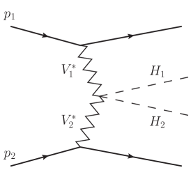
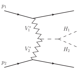
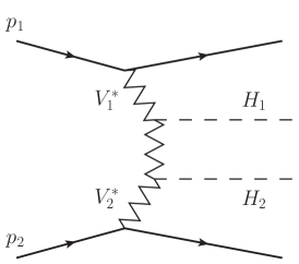
Figure 1: Born-level diagrams contributing to VBF Higgs pair production.

Because of the important role that double Higgs production via VBF will play at the LHC and beyond, substantial efforts have been made to calculate its cross section to high accuracy. The differential cross section has been calculated up to next-to-leading order (NLO) Figy (2008); Baglio et al. (2013) with matching to parton shower Frederix et al. (2014), and up to next-to-next-to-leading order when integrating out all hadronic final states Ling et al. (2014).

We present here the calculation of di-Higgs production up to next-to-next-to-next-to-leading order (N³LO), which is also the first calculation at this order of a $2\to 4$ process. Together with a companion paper presenting the fully differential NNLO calculation Dreyer and Karlberg (2018), this brings the VBF double Higgs channel to the same theoretical accuracy as single-Higgs VBF production Bolzoni et al. (2010); Cacciari et al. (2015); Dreyer and Karlberg (2016); Cruz-Martinez et al. (2018). These results are obtained using the structure function approach Han et al. (1992), which is the limit in which there is no partonic exchange between the two protons, and in which all radiation has been integrated over. Since the single-gluon exchange is zero for color reasons, this approximation is exact at NLO, while it has been shown to be accurate to more than 1% at NNLO for the single-Higgs process Ciccolini et al. (2008); Harlander et al. (2008); Bolzoni et al. (2012). Because the presence of an additional Higgs boson does not impact the color flow between the hadrons, this limit is expected to be just as valid for Higgs pair production.

This paper is structured in the following way: In section II we present the details of our calculation, in section III we present results for the inclusive cross section, while differential distributions are given in section IV. We give our conclusions in section V.

II Higgs pair production in VBF

We start by setting up the formalism needed to calculate the inclusive cross section up to third order in the expansion in the strong coupling constant, which is analogous to the single-Higgs one.

The VBF Higgs pair production cross section is calculated as a double deep inelastic scattering (DIS) process, and can be written as Han et al. (1992)

$$d\sigma= \,\sum_{V}\frac{G_{F}^{2}m_{V}^{4}}{s}\Delta_{V}^{2}(Q_{1}^{2})\Delta_{V}^{2}(Q_{2}^{2})\,d\Omega_{\text{VBF}}$$

$$\times\mathcal{W}^{V}_{\mu\nu}(x_{1},Q_{1}^{2})\mathcal{M}^{V,\mu\rho}\mathcal{M}^{V*,\nu\sigma}\mathcal{W}^{V}_{\rho\sigma}(x_{2},Q_{2}^{2})\,.$$ (1)

Here $G_{F}$ is Fermi’s constant, $m_{V}$ and $\Delta_{V}^{2}$ are the mass and squared propagators of the mediating $W$ or $Z$ bosons, and $\sqrt{s}$ is the collider center-of-mass energy. We defined $Q_{i}^{2}=-q_{i}^{2}$ and $x_{i}=Q_{i}^{2}/(2P_{i}\cdot q_{i})$ as the usual DIS variables, where $q_{i}$ is the four-momentum of the vector boson $V_{i}$ and $P_{i}$ that of the initial proton. Finally $\mathcal{W}^{V}_{\mu\nu}$ is the hadronic tensor and $d\Omega_{\text{VBF}}$ is the four particle VBF phase space. The matrix element of the $VV\to hh$ sub-process is expressed as Dobrovolskaya and Novikov (1991)

$$\mathcal{M}^{V,\mu\nu}=2\sqrt{2}G_{F}g^{\mu\nu}\bigg{(}\frac{2m_{V}^{4}}{(q_{1}+k_{1})^{2}-m_{V}^{2}+i\Gamma_{V}m_{V}}+\frac{2m_{V}^{4}}{(q_{1}+k_{2})^{2}-m_{V}^{2}+i\Gamma_{V}m_{V}}+\frac{6\nu\lambda m_{V}^{2}}{(k_{1}+k_{2})^{2}-m_{H}^{2}+i\Gamma_{H}m_{H}}+m_{V}^{2}\bigg{)}\\ +\frac{\sqrt{2}G_{F}m_{V}^{4}}{(q_{1}+k_{1})^{2}-m_{V}^{2}}\frac{(2k_{1}^{\mu}+q_{1}^{\mu})(k_{2}^{\nu}-k_{1}^{\nu}-q_{1}^{\nu})}{m_{V}^{2}-i\Gamma_{V}m_{V}}+\frac{\sqrt{2}G_{F}m_{V}^{4}}{(q_{1}+k_{2})^{2}-m_{V}^{2}}\frac{(2k_{2}^{\mu}+q_{1}^{\mu})(k_{1}^{\nu}-k_{2}^{\nu}-q_{1}^{\nu})}{m_{V}^{2}-i\Gamma_{V}m_{V}}\,,$$ (2)

where $k_{1},k_{2}$ are the final state Higgs momenta, which satisfy $k_{1}+k_{2}=q_{1}+q_{2}$, $\lambda$ is the trilinear Higgs self-coupling and $\nu$ is the vacuum expectation value of the Higgs field.

Defining $\hat{P}_{i,\mu}=P_{i,\mu}-\tfrac{P_{i}\cdot q_{i}}{q_{i}^{2}}q_{i,\mu}$, the hadronic tensor $\mathcal{W}^{V}_{\mu\nu}$ in equation (II) is given by

$$\mathcal{W}^{V}_{\mu\nu}(x_{i},Q_{i}^{2})=\Big{(}-g_{\mu\nu}+\frac{q_{i,\mu}q_{i,\nu}}{q_{i}^{2}}\Big{)}F_{1}^{V}(x_{i},Q_{i}^{2})\\ +\frac{\hat{P}_{i,\mu}\hat{P}_{i,\nu}}{P_{i}\cdot q_{i}}F_{2}^{V}(x_{i},Q_{i}^{2})+i\epsilon_{\mu\nu\rho\sigma}\frac{P_{i}^{\rho}q_{i}^{\sigma}}{2P_{i}\cdot q_{i}}F_{3}^{V}(x_{i},Q_{i}^{2})\,,$$ (3)

where the $F^{V}_{i}(x,Q^{2})$ functions are the standard DIS structure functions with $i=1,2,3$, which can be expressed as a convolution of the parton distribution functions (PDF) with the short distance coefficient functions

$$F_{i}^{V}=\sum_{a=q,g}C_{i}^{V,a}\otimes f_{a}\,,\quad i=1,2,3\,.$$ (4)

To evaluate equation (4), it is useful to define the singlet and non-singlet distributions $q_{\text{S}}\,,q_{\text{NS},i}$, as well as the non-singlet valence distribution $q_{\text{NS}}^{V}$ and the asymmetry $\delta q_{\text{NS}}^{\pm}$

$$q_{\text{S}}=\sum_{j=1}^{n_{f}}(q_{j}+\bar{q}_{j}),\;\;q_{\text{NS},j}^{\pm}=q_{j}\pm\bar{q}_{j},\;\;q_{\text{NS}}^{v}=\sum_{j=1}^{n_{f}}(q_{j}-\bar{q}_{j}),$$

$$\delta q_{\text{NS}}^{\pm}=\sum_{u\text{-type}}(q_{j}\pm\bar{q}_{j})-\sum_{d\text{-type}}(q_{j}\pm\bar{q}_{j})\,.$$ (5)

We can then decompose the quark coefficient functions into non-singlet and pure-singlet parts, and define the valence coefficient function

$$C_{L,q}=C^{+}_{L,\text{NS}}+C_{L,\text{PS}}\,,\quad C_{2,q}=C^{+}_{2,\text{NS}}+C_{2,\text{PS}}\,,$$

$$C^{v}_{3,\text{NS}}=C^{-}_{3,\text{NS}}+C^{s}_{3,\text{NS}}\,,$$ (6)

The neutral current structure functions can now be expressed as

$$F_{i}^{Z}(x)=2x\int_{0}^{1}dz\int_{0}^{1}dy\delta(x-yz)\sum_{j=1}^{n_{f}}\big{[}(v^{Z}_{j})^{2}+(a^{Z}_{j})^{2}\big{]}\\ \times\Big{[}q^{+}_{\text{NS},j}(y)C_{i,\text{NS}}^{+}(z)+q_{\text{S}}(y)C_{i,\text{PS}}(z)+g(y)C_{i,g}(z)\Big{]},$$ (7)

$$F_{3}^{Z}(x)=4\int_{0}^{1}dz\int_{0}^{1}dy\delta(x-yz)\sum_{j=1}^{n_{f}}v^{Z}_{j}a^{Z}_{j}\\ \times\Big{[}q_{\text{NS},j}^{-}(y)C^{-}_{3,\text{NS}}(z)+q_{\text{NS}}^{v}(y)C_{3,\text{NS}}^{v}(z)\Big{]}\,,$$ (8)

where $i=2,L$ and $F_{1}^{Z}=\tfrac{1}{2x}(F_{2}^{Z}-F_{L}^{Z})$. The vector and axial-vector coupling constants $v^{Z}_{i}$ and $a^{Z}_{i}$ are given by

$$v^{Z}_{j}=\pm\frac{1}{2}\,,\quad a^{Z}_{j}=\left\{\begin{array}[]{cc}\frac{1}{2}-\frac{4}{3}\sin^{2}\theta_{w},&u\text{-type}\\ -\frac{1}{2}+\frac{2}{3}\sin^{2}\theta_{w},&d\text{-type}\end{array}\right.$$ (11)

For the charged current case, the structure functions can be written as

$$F_{i}^{W^{\pm}}(x)=\frac{x}{n_{f}}\int_{0}^{1}dz\int_{0}^{1}dy\delta(x-yz)\sum_{j=1}^{n_{f}}\big{[}(v^{W}_{j})^{2}+(a^{W}_{j})^{2}\big{]}\\ \times\Big{[}\mp\delta q_{\text{NS}}^{-}(y)C_{i,\text{NS}}^{-}(z)+q_{\text{S}}(y)C_{i,q}(z)+g(y)C_{i,g}(z)\Big{]},$$ (12)

$$F_{3}^{W^{\pm}}(x)=\frac{2}{n_{f}}\int_{0}^{1}dz\int_{0}^{1}dy\delta(x-yz)\sum_{j=1}^{n_{f}}v^{W}_{j}a^{W}_{j}\\ \times\Big{[}\mp\delta q_{\text{NS}}^{+}(y)C^{+}_{3,\text{NS}}(z)+q_{\text{NS}}^{v}(y)C_{3,\text{NS}}^{v}(z)\Big{]}\,,$$ (13)

where we have again $F_{1}^{W^{\pm}}=\tfrac{1}{2x}(F_{2}^{W^{\pm}}-F_{L}^{W^{\pm}})$, and the couplings are simply $a^{W}_{j}=v^{W}_{j}=\tfrac{1}{\sqrt{2}}$.

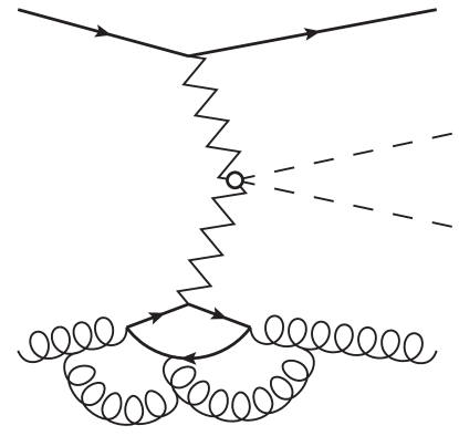
Figure 2: Three-loop diagrams contributing at N³LO to VBF Higgs pair production.

We can calculate corrections up to N³LO by making use of the known three-loop coefficient functions Moch et al. (2005); Vermaseren et al. (2005); Vogt et al. (2006); Moch et al. (2008); Davies et al. (2016), whose parameterized expressions have been implemented in HOPPET v1.2.0-struct-func-devel Salam and Rojo (2009). Examples of three-loop diagrams included in this calculation are shown in figure 2.

To calculate the variation of the cross section with different choices of factorization and renormalization scales, we compute the scale dependence to third order in the coefficient functions as well as in the PDFs.

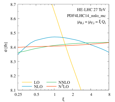
Figure 3: Total cross section as a function of the renormalization and factorization scales for each order in the perturbative expansion.

We start by evaluating the running coupling for $\alpha_{s}$

$$\alpha_{s}(Q)\simeq\alpha_{s}(\mu_{R})+\alpha_{s}^{2}(\mu_{R})\beta_{0}\ln\Big{(}\frac{\mu_{R}^{2}}{Q^{2}}\Big{)}\\ +\alpha_{s}^{3}(\mu_{R})\bigg{[}\beta_{0}^{2}\ln^{2}\Big{(}\frac{\mu_{R}^{2}}{Q^{2}}\Big{)}+\beta_{1}\ln\Big{(}\frac{\mu_{R}^{2}}{Q^{2}}\Big{)}\bigg{]}\,,$$ (14)

where we defined $\beta_{0}=(33-2n_{f})/12\pi$ and $\beta_{1}=(153-19n_{f})/24\pi^{2}$. The coefficient functions can then easily be expressed as an expansion in $\alpha_{s}(\mu_{R})$. To evaluate the dependence of the PDFs on the factorization scale $\mu_{F}$, we can integrate the DGLAP equation, using

$$f(x,Q)=f(x,\mu_{F})-\int_{0}^{L_{FQ}}dL\frac{d}{dL}f(x,\mu)\,.$$ (15)

Expressing the PDF in terms of an expansion in $\alpha_{s}(\mu_{R})$ evaluated at $\mu_{F}$, it then straightforward to evaluate equation (4) for any choice of the renormalization and factorization scales up to N³LO.

To estimate the theoretical uncertainty due to missing higher order corrections, we calculate the envelope of seven different scale choices, taking

$$\mu_{R}=\xi_{R}\,\mu_{0}\,,\quad\mu_{F}=\xi_{F}\,\mu_{0}\,,\quad\xi_{R,F}\in\{\tfrac{1}{2},1,2\}\,,$$ (16)

where we keep $\tfrac{1}{2}\leq\mu_{R}/\mu_{F}\leq 2$ and $\mu_{0}$ is the central scale choice. We set the central renormalization and factorization scales to the vector boson virtuality of the corresponding sector, $Q_{1}$ or $Q_{2}$.

For the numerical integration, we use the phase space parameterization of VBFNLO Baglio et al. (2011). Unless otherwise specified the center-of-mass energy is set to the expected energy of the HE-LHC, which is 27 TeV. For all simulations, we use the PDF4LHC15_nnlo_mc set Butterworth et al. (2016) with a four-loop evolution of the strong coupling, starting from an initial condition $\alpha_{s}(M_{Z})=0.118$. We set the mass of the Higgs boson to $m_{H}=125\;\mathrm{GeV}$. The electroweak parameters are set to the PDG values Tanabashi et al. (2018), with $m_{W}=80.379\;\mathrm{GeV}$, $m_{Z}=91.1876\;\mathrm{GeV}$ and $G_{F}=1.16637\cdot 10^{-5}\;\mathrm{GeV}^{-2}$. The narrow-width approximation is used for the final state Higgs bosons, while Breit-Wigner distributions are used for internal bosons, taking $\Gamma_{W}=2.085\;\mathrm{GeV}$, $\Gamma_{Z}=2.4952\;\mathrm{GeV}$, and $\Gamma_{H}=4.030\cdot 10^{-3}\;\mathrm{GeV}$.

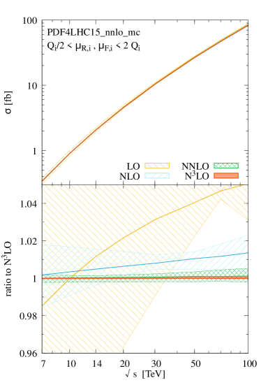
Figure 4: Total cross section as a function of energy for each order in perturbative QCD.

III Total cross section

We start by providing results for the inclusive cross section.

In figure 3, we show the dependence of the total cross section on the renormalization and factorization scales for each order in QCD. One can clearly observe the convergence of the perturbative expansion, with each order in $\alpha_{s}$ reducing the fluctuations due to changes in the choice of scale. We see that at N³LO there is almost no residual dependence on the scale, with predictions having an almost constant cross section over a broad range of scale values.

We show the dependence of the total cross section as a function of center-of-mass energy in figure 4. Here we see that at even very high energies, the third order corrections are fully contained within the NNLO scale variation bands, with an almost constant $K$-factor. One should note that this is somewhat dependent on the choice of central scale, and less dynamical scales such as an $m_{h}$ or $p_{t,HH}$ based prescription will lead to third order corrections that can deviate from the NNLO uncertainty bands in certain kinematic regions or at sufficiently high energies.

x $\sigma^{\text{(14 TeV)}}$ [fb] $\sigma^{\text{(27 TeV)}}$ [fb] $\sigma^{\text{(100 TeV)}}$ [fb] LO $2.079\,^{+0.177}_{-0.152}$ $8.651\,^{+0.411}_{-0.382}$ $87.104\,^{+1.023}_{-1.633}$ NLO $2.065\,^{+0.022}_{-0.018}$ $8.471\,^{+0.046}_{-0.024}$ $84.026\,^{+0.781}_{-0.860}$ NNLO $2.056\,^{+0.003}_{-0.005}$ $8.412\,^{+0.014}_{-0.021}$ $83.000\,^{+0.340}_{-0.269}$ N³LO $2.055\,^{+0.001}_{-0.001}$ $8.407\,^{+0.005}_{-0.003}$ $82.901\,^{+0.097}_{-0.035}$

Table 1: Total cross sections at LO, NLO, NNLO and N³LO for VBF Higgs pair production for different center-of-mass energies. The uncertainties are obtained from a seven-point scale variation.

We detail the precise value of the cross section and its scale variation uncertainties in table 1. Values are given for three reference center-of-mass energies: the 14 TeV LHC, the 27 TeV HE-LHC and the 100 TeV FCC. For each of these energies, we provide inclusive cross sections at each order in perturbative QCD, along with the corresponding scale variation envelope. We can observe that while the corrections are at the level of a few permille only, the scale uncertainty bands are reduced by more than a factor four when going from NNLO to N³LO.

A comment is due on the impact of contributions beyond those included in the DIS limit. There are a number of corrections to the Born diagrams shown in figure 1 beyond those due to the radiation of additional partons. These should be included where possible for precise phenomenological predictions.

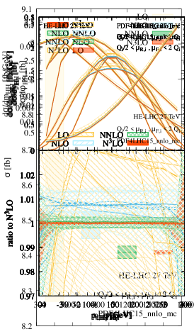
Figure 5: Differential cross sections for the transverse momentum $p_{t,HH}$, rapidity $y_{HH}$ and mass $m_{HH}$ distributions of the Higgs pair.

In particular, the $s$-channel production mode, while suppressed to a few permille after VBF cuts, contributes to about $16\%$ to the total cross section for 27 TeV collisions, and can therefore not be neglected. It can be calculated to NLO using the MadGraph5_aMC@NLO framework Alwall et al. (2014) and can be straightforwardly included.

Furthermore, NLO electroweak corrections are currently unknown and expected to be sizeable. They can be estimated from dominant light quark induced channels using Recola(Collier)+MoCaNLO Actis et al. (2017); Denner et al. (2017); Feger and Pellen (2015); Andersen et al. (2018) for the di-Higgs and single-Higgs VBF process, comparing the latter to HAWK Denner et al. (2015). For VBF Higgs pair production the EW corrections to the inclusive cross section lie between $-5\%$ and $-7\%$. Compared to the single-Higgs VBF correction of roughly $-5\%$ (using the same set-up, i.e. excluding photonic and b-quark channels), the double Higgs VBF process thus does not seem to receive large VBS-like corrections Biedermann et al. (2017a, b). One can therefore expect the full electroweak corrections to be at least at the same level as the NNLO QCD corrections, and significantly larger than the N³LO corrections.

There are also a number of $\alpha_{s}^{2}$ and $\alpha_{s}^{3}$ contributions that are neglected in the structure function approximation, notably: the double and triple gluon exchange between the two quark lines; heavy-quark loop induced production; $t$-/$u$-channel interferences; single-quark line contributions; loop induced interferences between VBF and gluon-fusion Higgs production. These have been shown to contribute at the few permille level in single Higgs VBF production Ciccolini et al. (2008); Andersen et al. (2008); Harlander et al. (2008); Bolzoni et al. (2012), and we therefore expect that they can be neglected.

The impact on the cross section of PDF and $\alpha_{s}$ uncertainties can be evaluated using the PDF4LHC15_nnlo_mc_pdfas set, and is of about $2.1\%$. Finally, there is also a theoretical PDF uncertainty, due to missing higher orders in the determination of the PDFs. In this paper we use an NNLO pdf set to evaluate an N³LO cross section, since N³LO sets are currently unavailable. The uncertainty due to these missing higher order terms come from two sources. They are dominated by missing third order corrections to the coefficient functions relating physical observables to PDFs, and can be estimated to about $8\permil$ using the method presented in Dreyer and Karlberg (2016). The second source of corrections is due to unknown four-loop splitting functions Vogt et al. (2018) appearing in the DGLAP evolution, which have been estimated to be negligible Dreyer and Karlberg (2016).

IV Differential distributions

The calculation described in section II is inclusive over final state QCD radiation. One can thus not obtain differential predictions with respect to the jet kinematics without using the projection-to-Born method Cacciari et al. (2015) and combining it with a higher multiplicity NNLO prediction. However, we have full access to the kinematics of the Higgs bosons, and it is therefore straightforward to compute differential observables with respect to the their momenta. Let us now focus on several differential distributions of particular interest. We will again consider here a 27 TeV proton-proton collider except where otherwise specified.

Figure 6: Differential cross sections for the transverse momentum distributions for both the harder ($p_{t,H_{1}}$) and softer ($p_{t,H_{2}}$) Higgs boson.

Figure 7: Differential cross sections for the rapidity distributions for both the harder ($y_{H_{1}}$) and softer ($y_{H_{2}}$) Higgs boson.

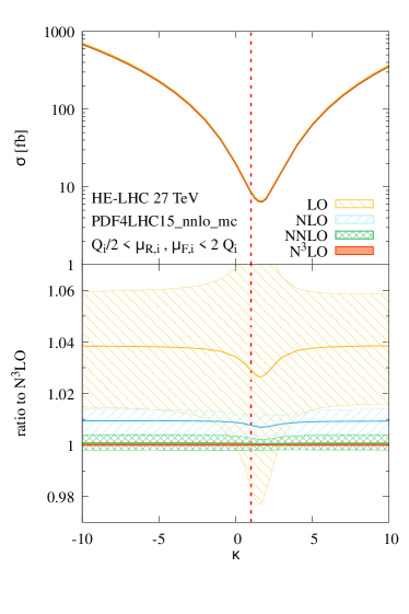
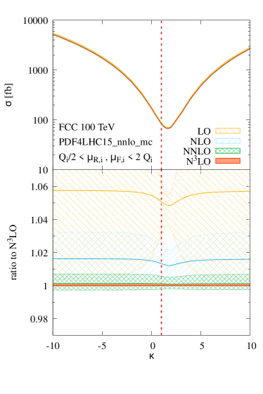
Figure 8: Total cross section as a function of $\kappa$ for both the 27 TeV HE-LHC (left) and the 100 TeV FCC (right). The lower panel gives the ratio to the central N³LOvalue, with scale uncertainty bands obtained from a seven-point variation.

In figure 5, we show the transverse momentum $p_{t,HH}$, rapidity $y_{HH}$ and invariant mass $m_{HH}$ distributions of the Higgs pair for each order in QCD. The latter is of particular interest, as the Higgs pair invariant mass can be notably sensitive to deviations due to physics beyond the SM Kaplan and Georgi (1984); Contino et al. (2010); Bishara et al. (2017). We see that once we get to the third order, there is almost no kinematic dependence to the $K$-factor, except at very high rapidities, where the N³LO corrections can bring changes to the central value of about one percent. The N³LO scale variation bands are always fully contained within the NNLO scale uncertainties, but are about four times thinner.

We order the Higgs bosons according to their transverse momentum. Figure 6 provides the transverse momentum distribution of both the harder ($p_{t,H_{1}}$) and the softer ($p_{t,H_{2}}$) Higgs. The third order corrections to these observables are negligible, with again a large reduction in scale uncertainties. The corrections to the rapidity distributions of the two Higgs bosons are shown in figure 7. We note here that the $\alpha_{s}^{3}$ contribution has almost no kinematic dependence up to rapidities of $|y_{H}|\sim 4$, with the scale variation bands being again fully contained by the theoretical uncertainties of the previous order.

Finally, let us study the impact of the trilinear Higgs self coupling, $\lambda$, by varying the corresponding factor in equation (2). Constraining the trilinear coupling is of particular interest, since many scenarios of new physics beyond the SM predict significant deviations of this value. Examples of such models are $SO(5)/SO(4)$ minimal composite Higgs Agashe et al. (2005); Contino et al. (2007) and dilaton models Goldberger et al. (2008).

To study the impact of deviations of this type, we define $\lambda=\kappa\lambda^{\text{SM}}$, where $\lambda^{\text{SM}}=m_{h}^{2}/2v$, and consider a range of values for $\kappa$.

The total cross section up to N³LO as a function of $\kappa$ is given in figure 8, both for a 27 TeV HE-LHC and for a 100 TeV FCC. One can observe that while the inclusive cross section changes by several orders of magnitude, there is as expected almost no dependence of the higher order corrections on $\kappa$ beyond leading order.

In figure 9, we show the kinematics of the Higgs pair for several values of $\kappa$. We see that even very small deviations in the trilinear Higgs coupling have a substantial impact on the cross sections, both in the normalization and shape of the distributions. In particular, the rapidity and invariant mass of the Higgs pair are particularly sensitive to changes in $\lambda$.

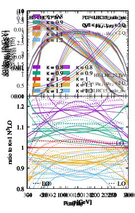
Figure 9: Differential cross sections for the transverse momentum $p_{t,HH}$, rapidity $y_{HH}$ and mass $m_{HH}$ distributions of the Higgs pair at N³LO for different values of the trilinear Higgs coupling $\lambda$. The lower panel gives the ratio to the central N³LO prediction with $\lambda=\lambda^{\text{SM}}$, with the LO shown as dashed lines. The bands correspond to theoretical scale uncertainties.

The lower panels in figure 9 show the ratio to the central value obtained with $\kappa=1$, with the leading order predictions shown as dashed lines. One can see that the changes to the cross sections from variations in $\kappa$ can be substantial. However there is essentially no change in the N³LO/LO $K$-factor.

V Conclusions

In this article, we have completed the first N³LO calculation of a $2\to 4$ process, namely the production of a Higgs boson pair through VBF. This calculation was made possible by the factorizable nature of the higher order QCD corrections. Together with the fully differential NNLO calculation presented in a companion paper Dreyer and Karlberg (2018), this brings the di-Higgs production channel to the same theoretical accuracy as has been achieved for the single-Higgs process, opening up the prospect of precision studies of the Higgs sector through Higgs pair production at the HE-LHC and at future hadron colliders.

We have presented differential distributions of the Higgs pair transverse momentum, rapidity and invariant mass for the 27 TeV HE-LHC. The corrections are at the few permille level, however the calculation of the third order leads to a substantial reduction in scale uncertainties. The convergence of the perturbative series is very stable at this order, with almost no kinematic dependence to the N³LO corrections, except at very high rapidities. The N³LO scale variation bands are always fully contained within the second order scale uncertainties, but are over four times thinner.

Finally we studied the impact of deviations from the SM in the trilinear Higgs self-coupling on the N³LO distributions. Small deviations of this constant can substantially change both the total cross section and the shape of the distributions. However the structure of the higher order QCD corrections is unaffected by variations in the coupling, with the N³LO/LO $K$-factor staying constant over a range broad range of $\lambda$ values.

The results presented here have been implemented in the version 2.0.0 of proVBFH-incl proVBFH-incl v2.0. which provides predictions for both single and double Higgs inclusive cross sections up to N³LO in QCD.

This article provides also the first element for a fully differential N³LO calculation of VBF Higgs pair production. This could be achieved by combining the present inclusive calculation with a differential NNLO computation of the electroweak production of two Higgs bosons in association with three jets.

Acknowledgments: We are grateful to Jean-Nicolas Lang and Mathieu Pellen for providing us with an estimate of the electroweak corrections. We also thank Gavin Salam and Giulia Zanderighi for their careful reading of the manuscript and useful comments. F.D. thanks the University of Zurich and the Pauli Center for Theoretical Studies, and A.K. thanks the University of Oxford and the Rudolf Peierls Centre for Theoretical Physics for hospitality while this work was being completed. F.D. is supported by the Science and Technology Facilities Council (STFC) under grant ST/P000770/1. A.K. is supported by the Swiss National Science Foundation (SNF) under grant number 200020-175595.

References

- Aad et al. (2012) G. Aad et al. (ATLAS), Phys. Lett. B716, 1 (2012), eprint 1207.7214.
- Chatrchyan et al. (2012) S. Chatrchyan et al. (CMS), Phys. Lett. B716, 30 (2012), eprint 1207.7235.
- Aaboud et al. (2018a) M. Aaboud et al. (ATLAS), Submitted to: Phys. Rev. Lett. (2018a), eprint 1808.00336.
- Aaboud et al. (2018b) M. Aaboud et al. (ATLAS), Submitted to: Eur. Phys. J. (2018b), eprint 1807.08567.
- Aaboud et al. (2018c) M. Aaboud et al. (ATLAS) (2018c), eprint 1807.04873.
- Aaboud et al. (2018d) M. Aaboud et al. (ATLAS) (2018d), eprint 1804.06174.
- Aaboud et al. (2016) M. Aaboud et al. (ATLAS), Phys. Rev. D94, 052002 (2016), eprint 1606.04782.
- Aad et al. (2015a) G. Aad et al. (ATLAS), Phys. Rev. D92, 092004 (2015a), eprint 1509.04670.
- Aad et al. (2015b) G. Aad et al. (ATLAS), Eur. Phys. J. C75, 412 (2015b), eprint 1506.00285.
- Aad et al. (2015c) G. Aad et al. (ATLAS), Phys. Rev. Lett. 114, 081802 (2015c), eprint 1406.5053.
- Sirunyan et al. (2018a) A. M. Sirunyan et al. (CMS) (2018a), eprint 1810.11854.
- Sirunyan et al. (2018b) A. M. Sirunyan et al. (CMS) (2018b), eprint 1806.00408.
- Sirunyan et al. (2018c) A. M. Sirunyan et al. (CMS), JHEP 01, 054 (2018c), eprint 1708.04188.
- Sirunyan et al. (2018d) A. M. Sirunyan et al. (CMS), Phys. Lett. B778, 101 (2018d), eprint 1707.02909.
- Sirunyan et al. (2017) A. M. Sirunyan et al. (CMS), Phys. Rev. D96, 072004 (2017), eprint 1707.00350.
- de Florian et al. (2016a) D. de Florian et al. (LHC Higgs Cross Section Working Group) (2016a), eprint 1610.07922.
- de Florian and Mazzitelli (2013) D. de Florian and J. Mazzitelli, Phys. Rev. Lett. 111, 201801 (2013), eprint 1309.6594.
- de Florian et al. (2016b) D. de Florian, M. Grazzini, C. Hanga, S. Kallweit, J. M. Lindert, P. Maierhöfer, J. Mazzitelli, and D. Rathlev, JHEP 09, 151 (2016b), eprint 1606.09519.
- de Florian and Mazzitelli (2015) D. de Florian and J. Mazzitelli, JHEP 09, 053 (2015), eprint 1505.07122.
- Grazzini et al. (2018) M. Grazzini, G. Heinrich, S. Jones, S. Kallweit, M. Kerner, J. M. Lindert, and J. Mazzitelli, JHEP 05, 059 (2018), eprint 1803.02463.
- Baglio et al. (2013) J. Baglio, A. Djouadi, R. Gröber, M. M. Mühlleitner, J. Quevillon, and M. Spira, JHEP 04, 151 (2013), eprint 1212.5581.
- Bishara et al. (2017) F. Bishara, R. Contino, and J. Rojo, Eur. Phys. J. C77, 481 (2017), eprint 1611.03860.
- Figy (2008) T. Figy, Mod. Phys. Lett. A23, 1961 (2008), eprint 0806.2200.
- Frederix et al. (2014) R. Frederix, S. Frixione, V. Hirschi, F. Maltoni, O. Mattelaer, P. Torrielli, E. Vryonidou, and M. Zaro, Phys. Lett. B732, 142 (2014), eprint 1401.7340.
- Ling et al. (2014) L.-S. Ling, R.-Y. Zhang, W.-G. Ma, L. Guo, W.-H. Li, and X.-Z. Li, Phys. Rev. D89, 073001 (2014), eprint 1401.7754.
- Dreyer and Karlberg (2018) F. A. Dreyer and A. Karlberg (2018), eprint 1811.07918.
- Bolzoni et al. (2010) P. Bolzoni, F. Maltoni, S.-O. Moch, and M. Zaro, Phys. Rev. Lett. 105, 011801 (2010), eprint 1003.4451.
- Cacciari et al. (2015) M. Cacciari, F. A. Dreyer, A. Karlberg, G. P. Salam, and G. Zanderighi, Phys. Rev. Lett. 115, 082002 (2015), [Erratum: Phys. Rev. Lett.120,no.13,139901(2018)], eprint 1506.02660.
- Dreyer and Karlberg (2016) F. A. Dreyer and A. Karlberg, Phys. Rev. Lett. 117, 072001 (2016), eprint 1606.00840.
- Cruz-Martinez et al. (2018) J. Cruz-Martinez, T. Gehrmann, E. W. N. Glover, and A. Huss, Phys. Lett. B781, 672 (2018), eprint 1802.02445.
- Han et al. (1992) T. Han, G. Valencia, and S. Willenbrock, Phys. Rev. Lett. 69, 3274 (1992), eprint hep-ph/9206246.
- Ciccolini et al. (2008) M. Ciccolini, A. Denner, and S. Dittmaier, Phys. Rev. D77, 013002 (2008), eprint 0710.4749.
- Harlander et al. (2008) R. V. Harlander, J. Vollinga, and M. M. Weber, Phys. Rev. D77, 053010 (2008), eprint 0801.3355.
- Bolzoni et al. (2012) P. Bolzoni, F. Maltoni, S.-O. Moch, and M. Zaro, Phys. Rev. D85, 035002 (2012), eprint 1109.3717.
- Dobrovolskaya and Novikov (1991) A. Dobrovolskaya and V. Novikov, Z. Phys. C52, 427 (1991).
- Moch et al. (2005) S. Moch, J. A. M. Vermaseren, and A. Vogt, Phys. Lett. B606, 123 (2005), eprint hep-ph/0411112.
- Vermaseren et al. (2005) J. A. M. Vermaseren, A. Vogt, and S. Moch, Nucl. Phys. B724, 3 (2005), eprint hep-ph/0504242.
- Vogt et al. (2006) A. Vogt, S. Moch, and J. Vermaseren, Nucl. Phys. Proc. Suppl. 160, 44 (2006), [,44(2006)], eprint hep-ph/0608307.
- Moch et al. (2008) S. Moch, M. Rogal, and A. Vogt, Nucl. Phys. B790, 317 (2008), eprint 0708.3731.
- Davies et al. (2016) J. Davies, A. Vogt, S. Moch, and J. A. M. Vermaseren, PoS DIS2016, 059 (2016), eprint 1606.08907.
- Salam and Rojo (2009) G. P. Salam and J. Rojo, Comput. Phys. Commun. 180, 120 (2009), eprint 0804.3755.
- Baglio et al. (2011) J. Baglio et al. (2011), eprint 1107.4038.
- Butterworth et al. (2016) J. Butterworth et al., J. Phys. G43, 023001 (2016), eprint 1510.03865.
- Tanabashi et al. (2018) M. Tanabashi et al. (Particle Data Group), Phys. Rev. D98, 030001 (2018).
- Alwall et al. (2014) J. Alwall, R. Frederix, S. Frixione, V. Hirschi, F. Maltoni, O. Mattelaer, H. S. Shao, T. Stelzer, P. Torrielli, and M. Zaro, JHEP 07, 079 (2014), eprint 1405.0301.
- Actis et al. (2017) S. Actis, A. Denner, L. Hofer, J.-N. Lang, A. Scharf, and S. Uccirati, Comput. Phys. Commun. 214, 140 (2017), eprint 1605.01090.
- Denner et al. (2017) A. Denner, S. Dittmaier, and L. Hofer, Comput. Phys. Commun. 212, 220 (2017), eprint 1604.06792.
- Feger and Pellen (2015) R. Feger and M. Pellen, MoCaNLO: a generic Monte Carlo event generator for NLO calculations of hadron-collider processes. (2015).
- Andersen et al. (2018) J. R. Andersen et al., in 10th Les Houches Workshop on Physics at TeV Colliders (PhysTeV 2017) Les Houches, France, June 5-23, 2017 (2018), eprint 1803.07977, URL http://lss.fnal.gov/archive/2018/conf/fermilab-conf-18-122-cd-t.pdf.
- Denner et al. (2015) A. Denner, S. Dittmaier, S. Kallweit, and A. Mück, Comput. Phys. Commun. 195, 161 (2015), eprint 1412.5390.
- Biedermann et al. (2017a) B. Biedermann, A. Denner, and M. Pellen, Phys. Rev. Lett. 118, 261801 (2017a), eprint 1611.02951.
- Biedermann et al. (2017b) B. Biedermann, A. Denner, and M. Pellen, JHEP 10, 124 (2017b), eprint 1708.00268.
- Andersen et al. (2008) J. R. Andersen, T. Binoth, G. Heinrich, and J. M. Smillie, JHEP 02, 057 (2008), eprint 0709.3513.
- Vogt et al. (2018) A. Vogt, F. Herzog, S. Moch, B. Ruijl, T. Ueda, and J. A. M. Vermaseren, PoS LL2018, 050 (2018), eprint 1808.08981.
- Kaplan and Georgi (1984) D. B. Kaplan and H. Georgi, Phys. Lett. 136B, 183 (1984).
- Contino et al. (2010) R. Contino, C. Grojean, M. Moretti, F. Piccinini, and R. Rattazzi, JHEP 05, 089 (2010), eprint 1002.1011.
- Agashe et al. (2005) K. Agashe, R. Contino, and A. Pomarol, Nucl. Phys. B719, 165 (2005), eprint hep-ph/0412089.
- Contino et al. (2007) R. Contino, L. Da Rold, and A. Pomarol, Phys. Rev. D75, 055014 (2007), eprint hep-ph/0612048.
- Goldberger et al. (2008) W. D. Goldberger, B. Grinstein, and W. Skiba, Phys. Rev. Lett. 100, 111802 (2008), eprint 0708.1463.
- proVBFH-incl v2.0. (0) proVBFH-incl v2.0.0, http://provbfh.hepforge.org/.