Measurements of the cosmological parameters $\Omega_{m}$, $\Omega_{k}$, $\Omega_{\textrm{\small{de}}}(a)$, $H_{0}$, and $\sum m_{\nu}$

Abstract

From Baryon Acoustic Oscillation measurements with Sloan Digital Sky Survey SDSS DR14 galaxies, and the acoustic horizon angle $\theta_{*}$ measured by the Planck Collaboration, we obtain $\Omega_{m}=0.2724\pm 0.0047$, and $h+0.020\cdot\sum{m_{\nu}}=0.7038\pm 0.0060$, assuming flat space and a cosmological constant. We combine this result with the 2018 Planck “TT,TE,EE$+$lowE$+$lensing” analysis, and update a study of $\sum m_{\nu}$ with new direct measurements of $\sigma_{8}$, and obtain $\sum m_{\nu}=0.27\pm 0.08$ eV assuming three nearly degenerate neutrino eigenstates. Measurements are consistent with $\Omega_{k}=0$, and $\Omega_{\textrm{\small{de}}}(a)=\Omega_{\Lambda}$ constant.

I Introduction and summary

From a study of Baryon Acoustic Oscillations (BAO) with Sloan Digital Sky Survey (SDSS) data release DR13 galaxies and the “sound horizon” angle $\theta_{\textrm{\tiny{MC}}}$ measured by the Planck Collaboration we obtained $\Omega_{m}=0.281\pm 0.003$ assuming flat space and a cosmological constant BH_ijaa . At the time, the 2016 Review of Particle Physics quoted $\Omega_{m}=0.308\pm 0.012$ PDG2016 . The new 2018 Planck “TT,TE,EE$+$lowE$+$lensing” measurement Planck obtains $\Omega_{m}=0.3153\pm 0.0073$, while the “TT,TE,EE$+$lowE$+$lensing$+$BAO” measurement obtains $\Omega_{m}=0.3111\pm 0.0056$ Planck . Due to the growing tension between these measurements, we decided to repeat the BAO analysis in Reference BH_ijaa , this time with SDSS DR14 galaxies.

The main difficulty with the BAO measurements is to distinguish the BAO signal from the cosmological and statistical fluctuations. The aim of the present analysis is to be very conservative by choosing large bins in redshift $z$ to obtain a larger significance of the BAO signal than in BH_ijaa . As a result, the present analysis is based on 6 independent BAO measurements, compared to 18 in BH_ijaa .

We assume flat space, i.e. $\Omega_{k}=0$, and constant dark energy density, i.e. $\Omega_{\textrm{\small{de}}}(a)=\Omega_{\Lambda}$, except in Tables 6, 7, and 8 that include more general cases. We assume three neutrino flavors with eigenstates with nearly the same mass, so $\sum m_{\nu}\approx 3m_{\nu}$. We adopt the notation of the Particle Data Group 2018 PDG2018 . All uncertainties have 68% confidence.

The analysis presented in this article obtains $\Omega_{m}=0.2724\pm 0.0047$ so the tension has increased further. We present full details of all fits to the galaxy-galaxy distance histograms of the present measurement so that the reader may cross-check each step of the analysis. Calibrating the BAO standard ruler we obtain $h+0.020\cdot\sum{m_{\nu}}=0.7038\pm 0.0060$.

Combining the direct measurement $\Omega_{m}=0.2724\pm 0.0047$ with the 2018 Planck “TT,TE,EE$+$lowE$+$lensing” analysis obtains $\Omega_{m}=0.2853\pm 0.0040$ and $h=0.6990\pm 0.0030$, at the cost of an increase of the Planck $\chi^{2}_{\textrm{\tiny{P}}}$ from 12956.78 to 12968.64.

Finally, we update the measurement of $\sum m_{\nu}$ of Reference BH_ijaa_3 with the data of this Planck$+\Omega_{m}$ combination, and two new direct measurements of $\sigma_{8}$, and obtain $\sum m_{\nu}=0.27\pm 0.08$ eV. This result is sensitive to the accuracy of the direct measurements of $\sigma_{8}$.

II Measurement of $\Omega_{m}$ with BAO as an uncalibrated standard ruler

We measure the comoving galaxy-galaxy correlation distance $d_{\textrm{\small{drag}}}$, in units of $c/H_{0}$, with galaxies in the Sloan Digital Sky Survey SDSS DR14 publicly released catalog SDSS_DR14 ; BOSS , with the method described in Reference BH_ijaa . Briefly, from the angle $\alpha$ between two galaxies as seen by the observer, and their red-shifts $z_{1}$ and $z_{2}$, we calculate their distance $d$, in units of $c/H_{0}$, assuming a reference cosmology BH_ijaa . At this “uncalibrated” stage in the analysis, the unit of distance $c/H_{0}$ is neither known nor needed. The adimensional distance $d$ has a component $d_{\alpha}$ transverse to the line of sight, and a component $d_{z}$ along the line of sight, given by Equation (3) of BH_ijaa . We fill three histograms of $d$ according to the orientation of the galaxy pairs with respect to the line of sight, i.e. $d_{z}/d_{\alpha}<1/3$, $d_{\alpha}/d_{z}<1/3$, and remaining pairs. Fitting these histograms we obtain excesses centered at $\hat{d}_{\alpha}$, $\hat{d}_{z}$, and $\hat{d}_{/}$ respectively. Examples are shown in Figures 1 and 2. From each BAO observable $\hat{d}_{\alpha}$, $\hat{d}_{/}$, or $\hat{d}_{z}$ we recover $d_{\textrm{\small{drag}}}$ for any given cosmology with Equations (5), (6), or (7) of Ref. BH_ijaa . Requiring that $d_{\textrm{\small{drag}}}$ be independent of red shift $z$ and orientation we obtain the space curvature $\Omega_{k}$, the dark energy density $\Omega_{\textrm{\small{de}}}(a)$ as a function of the expansion parameter $a=1/(1+z)$, and the matter density $\Omega_{m}=1-\Omega_{\textrm{\small{de}}}(1)-\Omega_{k}-\Omega_{r}$. Full details can be found in BH_ijaa .

The challenge with these BAO measurements is to distinguish the BAO signal from the cosmological and statistical fluctuations of the background. Our strategy is three-fold: (i) redundancy of measurements with different cosmological fluctuations, (ii) pattern recognition of the BAO signal, and (iii) requiring all three fits for $\hat{d}_{\alpha}$, $\hat{d}_{/}$, and $\hat{d}_{z}$ to converge, and that the consistency relation $Q=\hat{d}_{/}/(\hat{d}_{\alpha}^{0.57}\hat{d}_{z}^{0.43})=1$ BH_ijaa be satisfied within $\pm 3\%$.

Regarding redundancy, we repeat the fits for the northern (N) and southern (S) galactic caps; we repeat the measurements for galaxy-galaxy (G-G) distances, galaxy-large galaxy (G-LG) distances, LG-LG distances, and galaxy-cluster (G-C) distances; and we fill histograms of $d$ with weights $0.033^{2}/d^{2}$ or $0.033^{2}F_{i}F_{j}/d^{2}$, where $F_{i}$ and $F_{j}$ are absolute luminosities; see BH_ijaa for details. In the present analysis we have off-set the bins of redshift $z$ with respect to Reference BH_ijaa to obtain different background fluctuations.

Now consider pattern recognition. Figures 1 and 2 show that the BAO signal is approximately constant from $\approx 0.032$ to $\approx 0.037$, corresponding to $\approx 137$ Mpc to $\approx 158$ Mpc. This characteristic shape of the BAO signal can be understood qualitatively with reference to Figure (1) of Eisenstein : the radial mass profile of an initial point like adiabatic excess results, well after recombination, in peaks at radii 17 Mpc and $r_{\textrm{\small{drag}}}\approx 148$ Mpc, so we can expect the BAO signal to extend from approximately $148-17$ Mpc to $148+17$ Mpc, with $r_{\textrm{\small{drag}}}$ at the mid-point. From galaxy simulations described in BH_ijaa_3 , the smearing of $r_{\textrm{\small{drag}}}$ due to galaxy peculiar motions has a standard deviation approximately 7.6 Mpc at $z=0.5$, and 8.5 Mpc at $z=0.3$. So the observed BAO signal has an unexpected “step-up-step-down” shape, and is narrower than implied by the simulation in reference Eisenstein .

The selections of galaxies are as in BH_ijaa with the added requirements for SDSS DR14 galaxies that they be “sciencePrimary” and “bossPrimary”, and have a smaller redshift uncertainty zErr$<0.00025$.

The fitting function has 6 free parameters, corresponding to a second degree polynomial for the background, and a “smooth step-up-step-down” function (described in BH_ijaa ) with a center $\hat{d}$, a half-width $\Delta$, and an amplitude $A$ relative to the background. Each fit used for the final measurements is required to have a significance $A/\sigma_{A}>2$ (in the analysis of BH_ijaa this requirement was $A/\sigma_{A}>1$, which allows more bins of $z$).

Successful triplets of fits are presented in Table 1. Note the redundancy of measurements with $0.250<z<0.425$ and $0.425<z<800$. The independent triplets of fits selected for further analysis, are indicated with a “$*$”, and are shown in Figures 1 and 2, with further details presented in Table 2. We note that each measurement of $\hat{d}_{\alpha}$, $\hat{d}_{/}$, or $\hat{d}_{z}$ in Table 1, together with the sound horizon angle $\theta_{*}$ obtained by the Planck experiment Planck , is a sensitive measurement of $\Omega_{m}$ as shown in Table 3.

The peculiar motion corrections were studied with the galaxy generator described in BH_ijaa_3 ; BH_galaxies . Results of these simulations are shown in Table 4, for G-G distances, for two cases: “correct $P(k)$” and “correct $P_{\textrm{gal}}(k)$”. The “correct $P(k)$” simulations have the predicted linear power spectrum of density fluctuations $P(k)$ of the $\Lambda$CDM model (Eq. (8.1.42) of Weinberg ), while the “correct $P_{\textrm{gal}}(k)$” simulations have a steeper $P(k)$ input so that the generated galaxy power spectrum $P_{\textrm{gal}}(k)$ matches observations, see Figure (15) of BH_ijaa_3 . (The need for the steeper $P(k)$ is currently not understood.) All of these G-G corrections, and also the corrections for LG-LG and G-C, are in agreement, to within a factor 2, with the corrections applied in BH_ijaa that where taken from a study in Seo . In summary, in the present analysis we apply the same peculiar motion corrections as in BH_ijaa , i.e. we multiply the measured BAO distances $\hat{d}_{\alpha}$, $\hat{d}_{/}$, and $\hat{d}_{z}$, by correction factors $f_{\alpha}$, $f_{/}$, and $f_{z}$, respectively, where

$$f_{\alpha}-1 = 0.00320\cdot a^{1.35},$$

$$f_{/}-1 = 0.00350\cdot a^{1.35},$$

$$f_{z}-1 = 0.00381\cdot a^{1.35}.$$ (1)

We take half of these corrections as a systematic uncertainty. The effect of these corrections is relatively small as shown in Table 6 below.

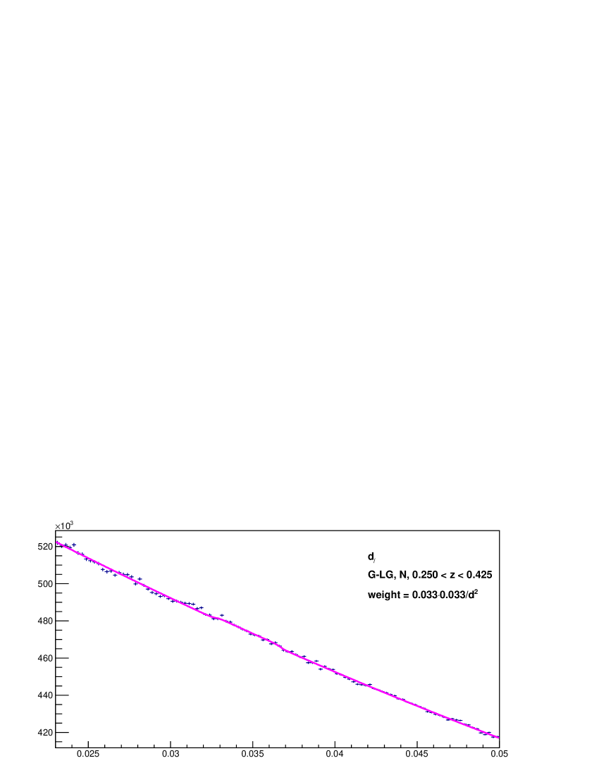
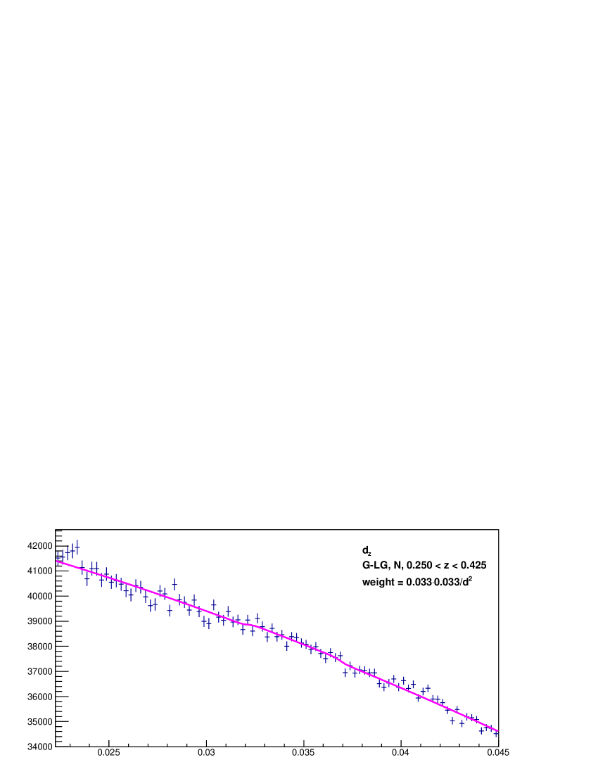
Figure 1: Fits to histograms of G-LG distances $d$ that obtain $\hat{d}_{\alpha}$, $\hat{d}_{/}$, or $\hat{d}_{z}$ at $z=0.34$. See Tables 1 and 2 for details.

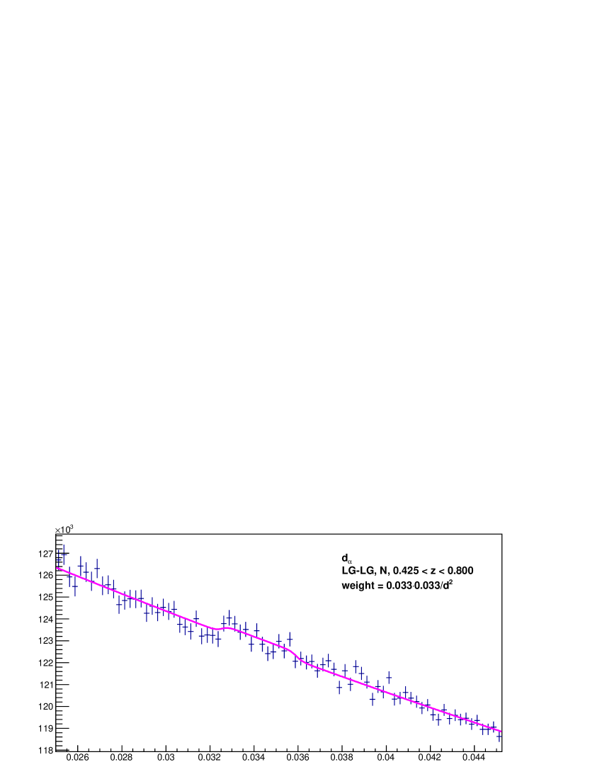
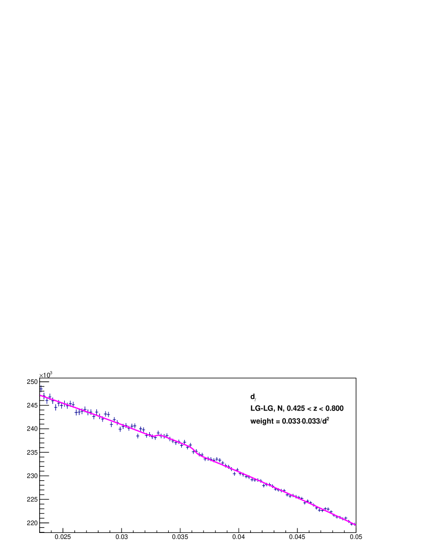
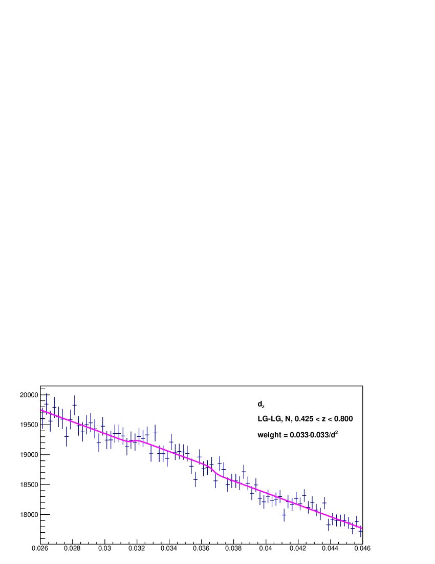
Figure 2: Fits to histograms of LG-LG distances $d$ that obtain $\hat{d}_{\alpha}$, $\hat{d}_{/}$, or $\hat{d}_{z}$ at $z=0.56$. See Tables 1 and 2 for details.

Table 1: Measured BAO distances $\hat{d}_{\alpha}$, $\hat{d}_{/}$, and $\hat{d}_{z}$, in units of $c/H_{0}$, with $z_{c}=3.79$ (see BH_ijaa ) from SDSS DR14 galaxies with right ascension $110^{0}$ to $270^{0}$, and declination $-5^{0}$ to $70^{0}$, in the northern (N) and/or southern (S) galactic caps. Uncertainties are statistical from the fits to the BAO signal. No corrections have been applied. The independent measurements with a “$*$” are selected for further analysis. The corresponding fits are presented in Figures 1 and 2, and details are presented in Table 2. For comparison, measurements with a “&” correspond to SDSS DR13 data with the galaxy selections of BH_ijaa .

$z$	$z_{\textrm{min}}$	$z_{\textrm{max}}$	Galaxies	Centers	Type	$100\hat{d}_{\alpha}$	$100\hat{d}_{/}$	$100\hat{d}_{z}$	Q
0.53	0.425	0.725	614724	614724	G-G, N$+$S	$3.488\pm 0.015$	$3.504\pm 0.019$	$3.466\pm 0.032$	1.007
0.53	0.425	0.725	614724	13960	G-C, N$+$S	$3.381\pm 0.030$	$3.401\pm 0.033$	$3.395\pm 0.035$	1.004
0.53	0.475	0.575	180696	53519	G-LG, N	$3.424\pm 0.015$	$3.314\pm 0.018$	$3.242\pm 0.018$	0.991
0.53	0.475	0.575	53519	53519	LG-LG, N	$3.451\pm 0.030$	$3.447\pm 0.059$	$3.351\pm 0.022$	1.012
0.53	0.475	0.575	180696	5045	G-C, N	$3.427\pm 0.031$	$3.331\pm 0.030$	$3.316\pm 0.033$	0.986
0.56	0.425	0.800	230841	230841	G-G, S	$3.441\pm 0.027$	$3.422\pm 0.017$	$3.497\pm 0.040$	0.988
0.56	0.425	0.800	355737	120499	G-LG, N	$3.425\pm 0.015$	$3.465\pm 0.016$	$3.351\pm 0.025$	1.021
$*$0.56	0.425	0.800	120499	120499	LG-LG, N	$3.424\pm 0.021$	$3.461\pm 0.018$	$3.424\pm 0.039$	1.011
&0.56	0.425	0.800	143778	143778	LG-LG, N	$3.424\pm 0.014$	$3.478\pm 0.015$	$3.451\pm 0.026$	1.012
0.56	0.425	0.800	586578	13206	G-C, N$+$S	$3.453\pm 0.038$	$3.365\pm 0.044$	$3.354\pm 0.028$	0.987
0.52	0.425	0.575	236693	236693	G-G, N	$3.437\pm 0.031$	$3.423\pm 0.026$	$3.432\pm 0.025$	0.997
0.52	0.425	0.575	236693	72297	G-LG, N	$3.416\pm 0.017$	$3.441\pm 0.012$	$3.385\pm 0.018$	1.011
0.52	0.425	0.575	72297	72297	LG-LG, N	$3.456\pm 0.033$	$3.447\pm 0.022$	$3.392\pm 0.060$	1.006
0.48	0.425	0.525	151938	4143	G-C, N	$3.424\pm 0.051$	$3.383\pm 0.026$	$3.343\pm 0.062$	0.998
0.36	0.250	0.450	114597	114597	G-G, N	$3.456\pm 0.018$	$3.386\pm 0.015$	$3.318\pm 0.056$	0.997
0.36	0.250	0.450	114597	65130	G-LG, N	$3.455\pm 0.010$	$3.358\pm 0.015$	$3.293\pm 0.032$	0.992
0.36	0.250	0.450	65130	65130	LG-LG, N	$3.462\pm 0.016$	$3.352\pm 0.025$	$3.307\pm 0.039$	0.988
0.34	0.250	0.425	92321	92321	G-G, N	$3.439\pm 0.013$	$3.473\pm 0.015$	$3.423\pm 0.076$	1.012
0.34	0.250	0.425	149849	149849	G-G, N$+$S	$3.437\pm 0.014$	$3.367\pm 0.013$	$3.444\pm 0.042$	0.979
$*$0.34	0.250	0.425	92321	55980	G-LG, N	$3.449\pm 0.008$	$3.471\pm 0.013$	$3.450\pm 0.034$	1.006
&0.34	0.250	0.425	133729	94873	G-LG, N	$3.431\pm 0.011$	$3.469\pm 0.014$	$3.383\pm 0.024$	1.017
0.34	0.250	0.425	55980	55980	LG-LG, N	$3.467\pm 0.019$	$3.477\pm 0.015$	$3.459\pm 0.045$	1.004

Table 2: Details of the fits selected for the final analysis (indicated by a “$*$” in Table 1). Note that the significance of the fitted signal amplitudes (relative to the background) range from 2.1 to 9.8 standard deviations.

Observable	$z$	Relative amplitude $A$	Half-width $\Delta$
$\hat{d}_{\alpha}$	0.56	$0.00290\pm 0.00100$	$0.00169\pm 0.00022$
$\hat{d}_{/}$	0.56	$0.00422\pm 0.00069$	$0.00164\pm 0.00020$
$\hat{d}_{z}$	0.56	$0.00505\pm 0.00226$	$0.00250\pm 0.00041$
$\hat{d}_{\alpha}$	0.34	$0.00632\pm 0.00064$	$0.00225\pm 0.00008$
$\hat{d}_{/}$	0.34	$0.00269\pm 0.00044$	$0.00197\pm 0.00013$
$\hat{d}_{z}$	0.34	$0.00341\pm 0.00162$	$0.00238\pm 0.00035$

Table 3: Calculated $d_{\textrm{\small{drag}}}$, $\hat{d}_{\alpha}$, $\hat{d}_{/}$, and $\hat{d}_{z}$ for $z=0.56$ and $z=0.34$, as a function of $\Omega_{m}$, for $\Omega_{k}=0$ and $\Omega_{de}(a)\equiv\Omega_{\Lambda}$ constant. $d_{\textrm{\small{drag}}}$ is the BAO galaxy comoving standard ruler length in units of $c/H_{0}$. It is calculated from $d_{\textrm{\small{drag}}}=1.0184d_{*}$, $d_{*}\equiv\theta_{*}\chi(z_{*})$, $\theta_{*}=0.0104092$, $\chi\equiv\int_{0}^{z_{*}}dz/E(z)$, $E(a)=(\Omega_{m}/a^{3}+\Omega_{r}/a^{4}+\Omega_{\Lambda}+\Omega_{k}/a^{2})^{1/2}$, and $a=1/(1+z)$. $\hat{d}_{\alpha}$, $\hat{d}_{/}$, and $\hat{d}_{z}$ are calculated with equations (5), (6), and (7) of [1] with $z_{c}=3.79$. The dependence on $h=0.7$ or $\sum m_{\nu}=0.27$ eV is negligible compared to the uncertainties in Table 5.

$\Omega_{m}$	$100d_{\textrm{\small{drag}}}$	$100\hat{d}_{\alpha}$	$100\hat{d}_{/}$	$100\hat{d}_{z}$	$100\hat{d}_{\alpha}$	$100\hat{d}_{/}$	$100\hat{d}_{z}$
		$z=0.56$			$z=0.34$
0.25	3.628	3.535	3.510	3.477	3.560	3.538	3.510
0.27	3.519	3.457	3.444	3.427	3.471	3.457	3.440
0.28	3.468	3.421	3.414	3.405	3.429	3.420	3.408
0.29	3.420	3.386	3.385	3.384	3.390	3.385	3.377
0.31	3.330	3.323	3.333	3.346	3.317	3.319	3.321
0.33	3.248	3.265	3.285	3.311	3.251	3.259	3.271

Table 4: Study of peculiar motion corrections to be added to the G-G measurements of $\hat{d}_{\alpha}$, $\hat{d}_{/}$, and $\hat{d}_{z}$ in Table 1, obtained from simulations.

$z$	Simulation	$\Delta\hat{d}_{\alpha}$	$\Delta\hat{d}_{/}$	$\Delta\hat{d}_{z}$
0.5	correct $P(k)$	0.000062	0.000080	0.000112
0.5	correct $P_{\textrm{gal}}(k)$	0.000096	0.000125	0.000175
0.3	correct $P(k)$	0.000063	0.000080	0.000111
0.3	correct $P_{\textrm{gal}}(k)$	0.000084	0.000107	0.000148

Table 5: Uncertainties of $\hat{d}_{\alpha}$, $\hat{d}_{/}$, and $\hat{d}_{z}$ at 68% confidence.

	$\hat{d}_{\alpha}$	$\hat{d}_{/}$	$\hat{d}_{z}$
Method	$\pm 0.00003$	$\pm 0.00004$	$\pm 0.00008$
Peculiar motion correction	$\pm 0.00004$	$\pm 0.00004$	$\pm 0.00005$
Cosmological et al. $+$
statistical fluctuations	$\pm 0.00029$	$\pm 0.00055$	$\pm 0.00070$
Total	$\pm 0.00030$	$\pm 0.00055$	$\pm 0.00071$

Uncertainties of $\hat{d}_{\alpha}$, $\hat{d}_{/}$, and $\hat{d}_{z}$ are presented in Table 5. These uncertainties are dominated by cosmological and statistical fluctuations, and are estimated from the root-mean-square fluctuations of many measurements, from the width of the distribution of $Q$, and from the issues discussed in the appendices.

Fits to the two independent selected triplets $\hat{d}_{\alpha}$, $\hat{d}_{/}$, and $\hat{d}_{z}$ indicated by a “$*$” in Table 1, with the uncertainties in Table 5, are presented in Table 6.

Four Scenarios are considered. In Scenario 1 the dark energy density is constant, i.e. $\Omega_{\textrm{\small{de}}}(a)=\Omega_{\Lambda}$. In Scenario 2 the observed acceleration of the expansion of the universe is due to a gas of negative pressure with an equation of state $w\equiv p/\rho<0$. We allow the index $w$ to be a function of $a$ Chevallier ; Linder : $w(a)=w_{0}+w_{a}(1-a)$. Scenario 3 is the same as Scenario 2, except that $w$ is constant, i.e. $w_{a}=0$. In Scenario 4 we assume $\Omega_{\textrm{\small{de}}}(a)=\Omega_{\textrm{\small{de}}}[1+w_{1}(1-a)]$.

Note in Table 6 that $\Omega_{k}$ is consistent with zero, and $\Omega_{\textrm{de}}(a)$ is consistent with being independent of the expansion parameter $a$. For $\Omega_{k}=0$ and $\Omega_{\textrm{\small{de}}}(a)\equiv\Omega_{\Lambda}$ constant we obtain from Table 6:

$$\Omega_{m}=0.288\pm 0.037,$$ (2)

with $\chi^{2}=1.0$ for 4 degrees of freedom.

Table 6: Cosmological parameters obtained from the 6 independent galaxy BAO measurements indicated with a “$*$” in Table 1 in several scenarios. Corrections for peculiar motions are given by Eq. (1) except, for comparison, the fit “1*” which has no correction. Scenario 1 has $\Omega_{\textrm{\small{de}}}(a)$ constant. Scenario 3 has $w=w_{0}$. Scenario 4 has $\Omega_{\textrm{\small{de}}}(a)=\Omega_{\textrm{\small{de}}}\left[1+w_{1}(1-a)\right]$.

	Scenario 1*	Scenario 1	Scenario 1	Scenario 3	Scenario 4	Scenario 4
$\Omega_{k}$	$0$ fixed	$0$ fixed	$0.267\pm 0.362$	$0$ fixed	$0$ fixed	$0.262\pm 0.383$
$\Omega_{\textrm{\small{de}}}+0.6\Omega_{k}$	$0.712\pm 0.037$	$0.712\pm 0.037$	$0.738\pm 0.050$	$0.800\pm 0.364$	$0.760\pm 0.151$	$0.745\pm 0.148$
$w_{0}$	n.a.	n.a.	n.a.	$-0.76\pm 0.65$	n.a.	n.a.
$w_{1}$	n.a.	n.a.	n.a.	n.a.	$0.71\pm 2.00$	$0.13\pm 2.77$
$100d_{\textrm{\small{drag}}}$	$3.48\pm 0.06$	$3.487\pm 0.052$	$3.48\pm 0.06$	$3.43\pm 0.16$	$3.42\pm 0.19$	$3.48\pm 0.21$
$\chi^{2}/$d.f.	$0.9/4$	$1.0/4$	$0.4/3$	$0.9/3$	$0.9/3$	$0.4/2$

Final calculations are done with fits and numerical integrations. Never-the-less, it is convenient to present approximate analytical expressions obtained from the numerical integrations for the case of flat space and a cosmological constant. At decoupling, $z_{*}=1089.92\pm 0.25$ from the Planck “TT,TE,EE$+$lowE$+$lensing” measurement Planck . The “angular distance” at decoupling is $D_{A}(z_{*})\equiv\chi(z_{*})a_{*}c/H_{0}$, with

$$\chi(z_{*})=3.2675\left(\frac{h+0.35\sum{m_{\nu}}}{0.7}\right)^{0.01}\left(\frac{0.28}{\Omega_{m}}\right)^{0.4},$$ (3)

which has negligible dependence on $h$ or $\sum{m_{\nu}}$.

From the Planck “TT,TE,EE$+$lowE$+$lensing” measurement Planck , $\theta_{*}=0.0104092\pm 0.0000031$. Then the comoving sound horizon at decoupling is $r_{*}\equiv d_{*}c/H_{0}$, with

$$d_{*}=\theta_{*}\chi(z_{*})=0.03401\left(\frac{0.28}{\Omega_{m}}\right)^{0.4}.$$ (4)

The BAO standard ruler for galaxies $r_{\textrm{\small{drag}}}$ is larger than $r_{*}$ because last scattering of electrons occurs after last scattering of photons due to their different number densities. In the present analysis, we take $r_{\textrm{\small{drag}}}\equiv d_{\textrm{\small{drag}}}c/H_{0}$ with

$$\frac{d_{\textrm{\small{drag}}}}{d_{*}}=1.0184\pm 0.0004,$$ (5)

from the Planck “TT,TE,EE$+$lowE$+$lensing” analysis, with the uncertainty from Equation (10) of Reference Planck . Note from (4) and Equation (10) of Reference Planck that (5) is insensitive to cosmological parameters, so the uncalibrated analysis decouples from $h$ or $\sum m_{\nu}$.

We can test (5) experimentally. From Table 6 we obtain $d_{\textrm{\small{drag}}}=0.03487\pm 0.00052$. From (4) and (2) we obtain $d_{*}=0.03363\pm 0.00174$, so the measured $d_{\textrm{\small{drag}}}/d_{*}=1.037\pm 0.056$.

To the 6 independent galaxy BAO measurements, we add the sound horizon angle $\theta_{*}$, and obtain the results presented in Table 7. Note that measurements are consistent with flat space and a cosmological constant. Note also that the constraint on $\Omega_{k}$ becomes tighter if $\Omega_{\textrm{de}}(a)$ is assumed constant, and that the constraint on $\Omega_{\textrm{de}}(a)$ becomes tighter if $\Omega_{k}$ is assumed zero. In the scenario of flat space and a cosmological constant we obtain

$$\Omega_{m}=0.2724\pm 0.0047,$$ (6)

with $\chi^{2}=1.2$ for 5 degrees of freedom. This is the final result of the present analysis.

Adding two measurements in the quasar Lyman-alpha forest BH_ijaa ; lyman ; lyman2 we obtain the results presented in Table 8. In particular, for flat space and a cosmological constant we obtain

$$\Omega_{m}=0.2714\pm 0.0047.$$ (7)

with $\chi^{2}=10.0$ for 7 degrees of freedom. Note that the Lyman-alpha measurements tighten the constraints on $\Omega_{k}$, $w_{0}$, $w_{1}$, and $w_{a}$.

As a cross-check of the $z$ dependence, from the 4 independent fits to $\hat{d}_{\alpha}$ at different redshifts $z$ presented in Figure 3, plus $\theta_{*}$, we obtain

$$\Omega_{m}=0.2745\pm 0.0040,$$ (8)

with $\chi^{2}=3.0$ for 3 degrees of freedom, for flat space and a cosmological constant.

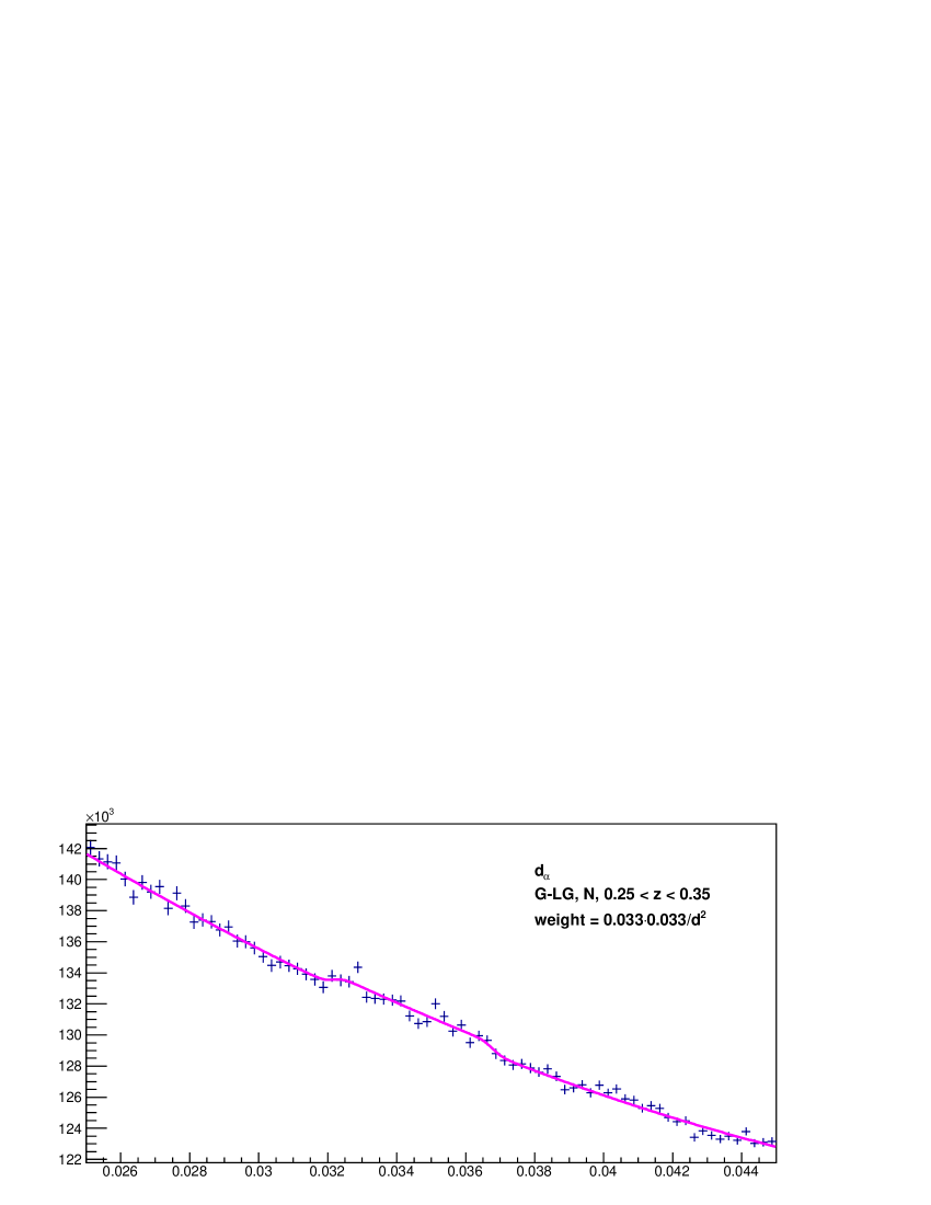
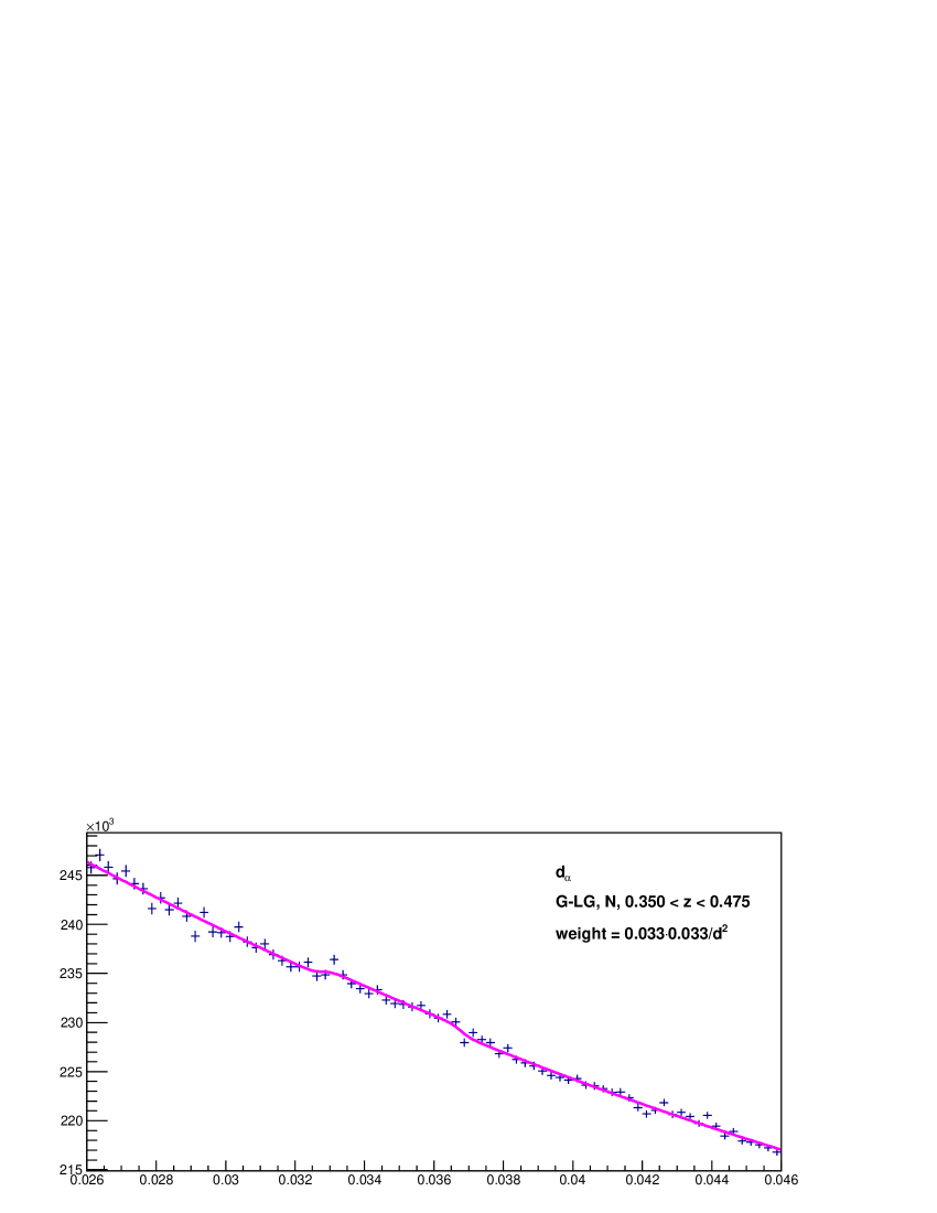
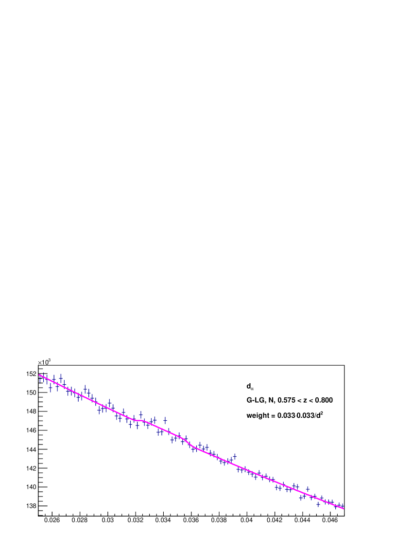
Figure 3: Fits to histograms of G-LG distances $d$ that obtain $\hat{d}_{\alpha}$ at $z=0.32,0.42,0.52$, and $0.65$. The bins of $z$ are $(0.25,0.35),(0.35,0.475),(0.475,0.575),\textrm{ and }(0.575,0.800)$, respectively. The fits obtain $\hat{d}_{\alpha}=0.03447\pm 0.00012,0.03478\pm 0.00012,0.03424\pm 0.00015,\textrm{ and }0.03399\pm 0.00020$ respectively, where uncertainties are statistical from the fits. A fit with these four measurements (with the total uncertainties of Table 5), plus $\theta_{*}$ from the Planck experiment, obtains $\Omega_{m}=0.2745\pm 0.0040$ and $d_{*}=0.03433\pm 0.00020$ with $\chi^{2}=3.0$ for 3 degrees of freedom.

As a cross-check of isotropy, from the 3 independent fits to $\hat{d}_{\alpha}$ at $z=0.36$ shown in Figure 4 corresponding to different regions of the sky, we obtain

$$\Omega_{m}=0.2737\pm 0.0043,$$ (9)

with $\chi^{2}=1.1$ for 2 degrees of freedom, for flat space and a cosmological constant.

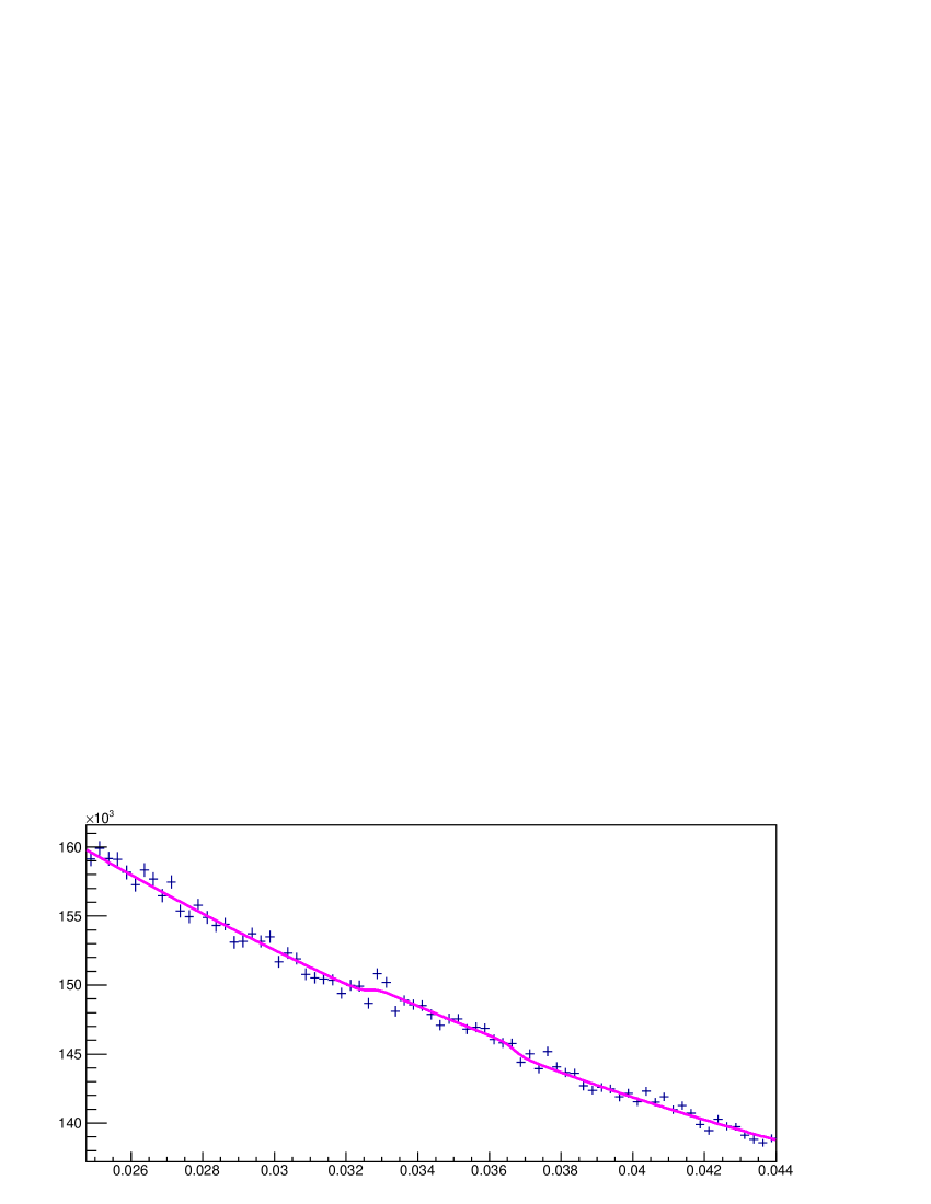
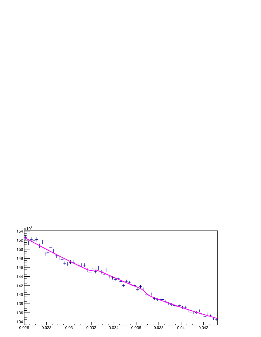
Figure 4: Fits to histograms of G-LG distances $d$, with $z$ in the range 0.25-0.45, that obtain $\hat{d}_{\alpha}$ at $z=0.36$. From top to bottom, they correspond to the northern galactic cap with right ascension $<180^{0}$ (NW), to the northern galactic cap with right ascension $>180^{0}$ (NE), and to the southern galactic cap (S). The fits obtain $\hat{d}_{\alpha}=0.03468\pm 0.00012,0.03447\pm 0.00012,\textrm{ and }0.03424\pm 0.00019$ respectively, where uncertainties are statistical from the fits. A fit with these three measurements (with the total uncertainties of Table 5), plus $\theta_{*}$ from the Planck experiment, obtains $\Omega_{m}=0.2737\pm 0.0043$ and $d_{*}=0.03437\pm 0.00022$ with $\chi^{2}=1.1$ for 2 degrees of freedom.

To check the stability of $\hat{d}_{\alpha}$, $\hat{d}_{/}$, and $\hat{d}_{z}$ with the data set and galaxy selections, we compare fits highlighted with “$*$” and “&” in Table 1, and also fits in Figure 6.

Additional studies are presented in the appendices.

Table 7: Cosmological parameters obtained from the 6 independent galaxy BAO measurements indicated with a “$*$” in Table 1, plus $\theta_{*}$ from the Planck experiment, in several scenarios. Corrections for peculiar motions are given by Eq. (1). $d_{\textrm{\small{drag}}}/d_{*}=1.0184\pm 0.0004$. Scenario 1 has $\Omega_{\textrm{\small{de}}}(a)$ constant. Scenario 2 has $w(a)=w_{0}+w_{a}(1-a)$. Scenario 3 has $w=w_{0}$. Scenario 4 has $\Omega_{\textrm{\small{de}}}(a)=\Omega_{\textrm{\small{de}}}\left[1+w_{1}(1-a)\right]$.

	Scenario 1	Scenario 1	Scenario 2	Scenario 3	Scenario 4	Scenario 4
$\Omega_{k}$	$0$ fixed	$0.008\pm 0.018$	$0$ fixed	$0$ fixed	$0$ fixed	$-0.007\pm 0.101$
$\Omega_{\textrm{\small{de}}}+2.1\Omega_{k}$	$0.7276\pm 0.0047$	$0.724\pm 0.009$	$0.708\pm 0.080$	$0.724\pm 0.008$	$0.723\pm 0.011$	$0.723\pm 0.011$
$w_{0}$	n.a.	n.a.	$-0.77\pm 1.47$	$-0.95\pm 0.10$	n.a.	n.a.
$w_{a}$ or $w_{1}$	n.a.	n.a.	$-0.91\pm 4.53$	n.a.	$0.19\pm 0.41$	$0.35\pm 2.20$
$100d_{*}$	$3.443\pm 0.024$	$3.42\pm 0.06$	$3.35\pm 0.04$	$3.41\pm 0.07$	$3.41\pm 0.09$	$3.39\pm 0.20$
$\chi^{2}/$d.f.	$1.2/5$	$1.0/4$	$0.9/3$	$1.0/4$	$1.0/4$	$1.0/3$

Table 8: Cosmological parameters obtained from the 6 galaxy BAO measurements indicated with a “$*$” in Table 1, plus $\theta_{*}$ from the Planck experiment, plus two Lyman-alpha measurements BH_ijaa ; lyman ; lyman2 in several scenarios. Corrections for peculiar motions are given by Eq. (1). $d_{\textrm{\small{drag}}}/d_{*}=1.0184\pm 0.0004$. Scenario 1 has $\Omega_{\textrm{\small{de}}}(a)$ constant. Scenario 2 has $w(a)=w_{0}+w_{a}(1-a)$. Scenario 3 has $w=w_{0}$. Scenario 4 has $\Omega_{\textrm{\small{de}}}(a)=\Omega_{\textrm{\small{de}}}\left[1+w_{1}(1-a)\right]$.

	Scenario 1	Scenario 1	Scenario 2	Scenario 3	Scenario 4	Scenario 4
$\Omega_{k}$	$0$ fixed	$-0.011\pm 0.008$	$0$ fixed	$0$ fixed	$0$ fixed	$-0.022\pm 0.010$
$\Omega_{\textrm{\small{de}}}+2.1\Omega_{k}$	$0.7286\pm 0.0047$	$0.734\pm 0.006$	$0.703\pm 0.028$	$0.726\pm 0.008$	$0.723\pm 0.011$	$0.720\pm 0.011$
$w_{0}$	n.a.	n.a.	$-0.70\pm 0.33$	$-0.96\pm 0.09$	n.a.	n.a.
$w_{a}$ or $w_{1}$	n.a.	n.a.	$-1.18\pm 1.37$	n.a.	$0.24\pm 0.40$	$0.80\pm 0.49$
$100d_{*}$	$3.449\pm 0.024$	$3.48\pm 0.04$	$3.32\pm 0.13$	$3.42\pm 0.07$	$3.40\pm 0.08$	$3.34\pm 0.09$
$\chi^{2}/$d.f.	$10.0/7$	$7.7/6$	$8.0/5$	$9.2/6$	$9.0/6$	$4.6/5$

III Measurement of $H_{0}$ with BAO as a calibrated standard ruler

We consider the scenario of flat space and a cosmological constant. It is useful to present approximate analytic expressions, tho all final calculations are done directly with fits to the measurements marked with a “$*$” in Table 1 and numerical integrations to obtain correct uncertainties for correlated parameters. To calibrate the BAO measurements, we integrate the comoving photon-electron-baryon plasma sound speed from $t=0$ up to decoupling and obtain the “comoving acoustic horizon distance” $r_{*}\equiv d_{*}c/H_{0}$, with

$$d_{*} = 0.03407\left(\frac{h+0.026\sum{m_{\nu}}}{0.7}\right)^{0.513}$$ (10)

$$\times\left(\frac{0.28}{\Omega_{m}}\right)^{0.244}\left(\frac{0.0225}{\Omega_{b}h^{2}}\right)^{0.097}.$$

The acoustic angular scale is

$$\theta_{*}\equiv\frac{d_{*}}{\chi(z_{*})} = 0.010427\left(\frac{h+0.020\sum m_{\nu}}{0.70}\right)^{0.503}$$ (11)

$$\times\left(\frac{\Omega_{m}}{0.28}\right)^{0.156}\left(\frac{0.0225}{\Omega_{b}h^{2}}\right)^{0.097},$$

in agreement with Equation (11) of Planck .

Let us now consider the measurement of $h$. From the galaxy BAO measurements in Table 6 we obtain $\Omega_{m}=0.288\pm 0.037$ and $d_{\textrm{\small{drag}}}=0.03487\pm 0.00052$. From Big Bang Nucleosynthesis, $\Omega_{b}h^{2}=0.0225\pm 0.0008$ at 68% confidence PDG2018 . From this data and Equations (5) and (10), or the corresponding fit, we obtain

$$h+0.026\sum{m_{\nu}}=0.716\pm 0.027,$$ (12)

with $\chi^{2}=1.0$ for 4 degrees of freedom.

The Planck measurement of $\theta_{*}$ allows a more precise measurement of $h$. From Table 7 we obtain $\Omega_{m}=0.2724\pm 0.0047$. Then from Big Bang Nucleosynthesis and (11), or the corresponding fit, we obtain

$$h+0.020\sum{m_{\nu}}=0.7038\pm 0.0060,$$ (13)

with $\chi^{2}=1.2$ for 5 degrees of freedom. Note that the uncertainties of $h$ and $\Omega_{m}$ are correlated through Equation (11).

IV Studies of CMB fluctuations

In Table 9 we present a qualitative study of the sensitivity of the CMB power spectrum $l(l+1)C_{TT,l}^{S}/(2\pi)$ to constrain $\Omega_{m}$ and $\sum m_{\nu}$. We use the approximate analytic expression (7.2.41) of Weinberg , modified to include $\sum m_{\nu}$, to compare the spectra with Planck 2018 “TT,TE,EE$+$lowE$+$lensing” parameters with the best fit spectra with fixed values $\Omega_{m}=0.2854$ and $\sum m_{\nu}=0.06,0.1,0.2,0.3,0.4,0.5$ eV. We find that the differences in spectra range from 0.11% to 0.3% of the first acoustic peak, see Figure 5. So the CMB power spectrum, while being very sensitive to constrain $\theta_{*}$, has low sensitivity to constrain $\Omega_{m}$ or $\sum m_{\nu}$.

Table 9: Cosmologies with fixed $\Omega_{m}$ and $\sum m_{\nu}$ fitted to the CMB power spectrum $l(l+1)C_{TT,l}^{S}/(2\pi)$ with the Planck 2018 “TT,TE,EE$+$lowE$+$lensing” parameters $\Omega_{m}=0.3153$, $\sum m_{\nu}=0.06$ eV, $h=0.6736$, $\Omega_{b}h^{2}=0.02237$, $n_{s}=0.9649$, $N^{2}=1.670\times 10^{-10}$, and $\tau=0.0544$ Planck . The approximate analytic equation (7.2.41) of Weinberg (modified to include $\sum m_{\nu}$) was used. Notation: $N^{2}\equiv A_{s}/(4\pi)\equiv\Delta_{R}^{2}/(4\pi)$.

$\Omega_{m}$	0.2854	0.2854	0.2854	0.2854	0.2854	0.2854
$\sum m_{\nu}$ [eV]	0.06	0.1	0.2	0.3	0.4	0.5
$h$	0.6980	0.6976	0.6965	0.6954	0.6942	0.6931
$100\Omega_{b}h^{2}$	2.282	2.288	2.306	2.324	2.343	2.362
$n_{s}$	0.9692	0.9699	0.9716	0.9735	0.9754	0.9774
$10^{10}N^{2}$	1.730	1.729	1.725	1.722	1.716	1.713
$\tau$	0.0774	0.0778	0.0787	0.0797	0.0799	0.0809
r.m.s. $[\mu\textrm{K}^{2}]$	6.07	6.98	9.29	11.66	14.06	16.49

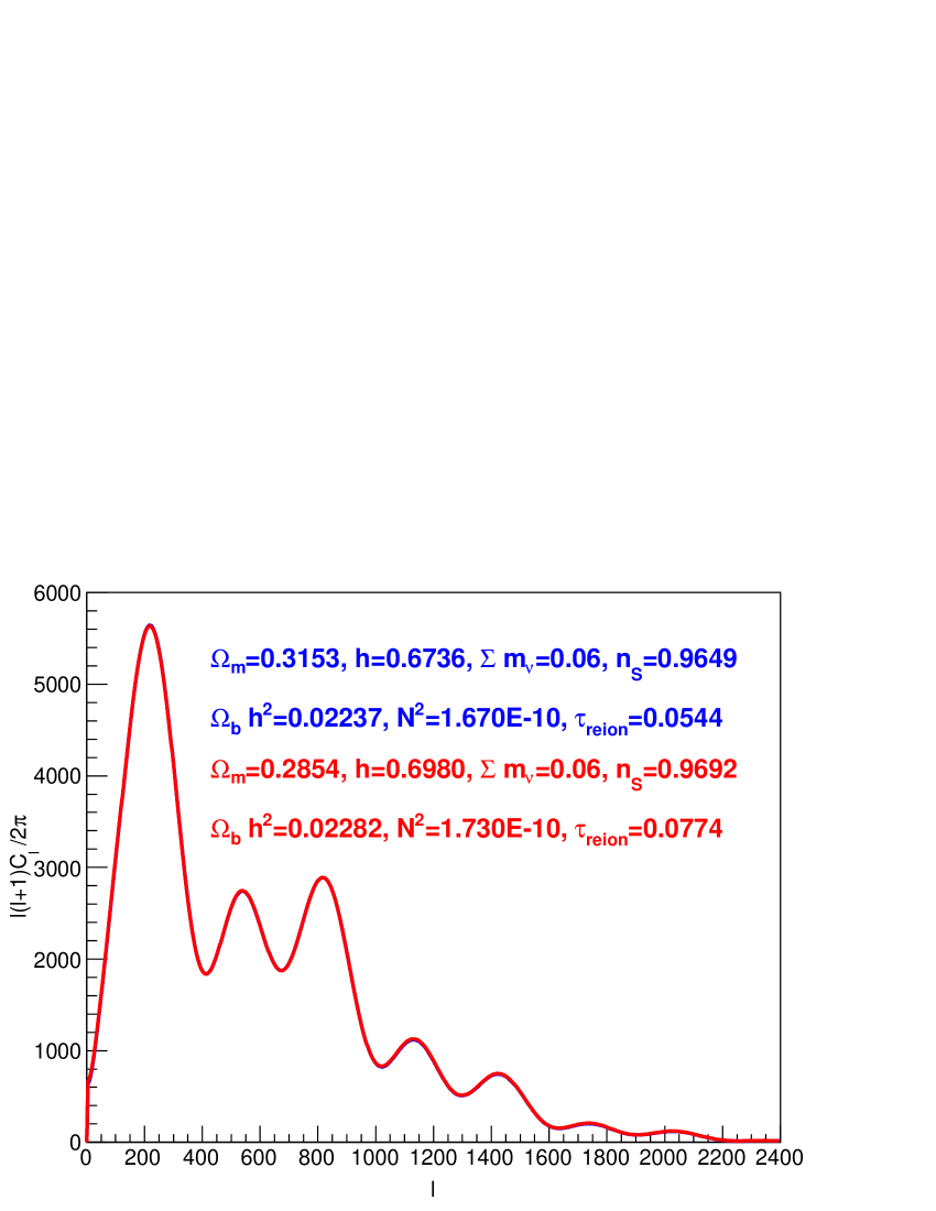
Figure 5: Comparison of the power spectra $l(l+1)C_{TT,l}^{S}/(2\pi)$ $[\mu\textrm{K}^{2}]$ for the Planck 2018 “TT,TE,EE$+$lowE$+$lensing” parameters, with the best fit spectra with $\Omega_{m}=0.2854$ and $\sum m_{\nu}=0.06$ eV fixed, calculated with the approximate Equation (7.2.41) of Weinberg (modified to include $\sum m_{\nu}$). The r.m.s. difference is $6.07\mu\textrm{K}^{2}$, corresponding to 0.11% of the first acoustic peak, so the two spectra can not be distinguished by eye.

In view of the low sensitivity of the CMB power spectra to constrain $\Omega_{m}$, the Planck analysis can benefit from a combination with the direct measurement of $\Omega_{m}$ given by Equation (6). The combination, obtained with the “base_mnu_plikHM_TTTEEE_lowTEB_lensing_*.txt MC chains” made public by the Planck Collaboration Planck , is presented in Table 10. This combination is preliminary due to the sparseness of the MC chains at low values of $\Omega_{m}$.

Table 10: Combination of the Planck 2018 “TT,TE,EE$+$lowE$+$lensing” analysis Planck with the directly measured $\Omega_{m}=0.2724\pm 0.0047$. Uncertainties are at $68\%$ confidence. The Planck $\chi^{2}_{\textrm{\tiny{P}}}\equiv-2\cdot\ln\mathcal{L}$ increases from 12956.78 to 12968.64 with this combination. The galaxy $\chi^{2}_{\textrm{\tiny{G}}}\equiv(\Omega_{m}-0.2724)^{2}/0.0047^{2}$. Preliminary.

	Planck	Planck$+\Omega_{m}$
$\Omega_{b}h^{2}$	$0.02237\pm 0.00015$	$0.02265\pm 0.00012$
$\Omega_{c}h^{2}$	$0.1200\pm 0.0012$	$0.1155\pm 0.0005$
$100\theta_{*}$	$1.04092\pm 0.00031$	$1.04125\pm 0.00022$
$\tau$	$0.0544\pm 0.0073$	$0.078\pm 0.006$
$\ln 10^{10}A_{s}$	$3.044\pm 0.014$	$3.102\pm 0.020$
$n_{s}$	$0.9649\pm 0.0042$	$0.9726\pm 0.0017$
$\Omega_{\Lambda}$	$0.6847\pm 0.0073$	$0.7147\pm 0.0040$
$\Omega_{m}$	$0.3153\pm 0.0073$	$0.2853\pm 0.0040$
$h$	$0.6736\pm 0.0054$	$0.6990\pm 0.0030$
$\sigma_{8}$	$0.8111\pm 0.0060$	$0.8346\pm 0.0054$
$\chi^{2}_{\textrm{\tiny{P}}}$	12956.78	12968.64
$\chi^{2}_{\textrm{\tiny{G}}}$	83.31	7.53
$\chi^{2}_{\textrm{tot}}$	13040.09	12976.17

V Tensions

We consider four direct measurements: (i) $h=0.7348\pm 0.0166$ by the Sh₀es Team Shoes , (ii) $\sigma_{8}\approx\left[0.746\pm 0.012\textrm{ (stat)}\pm 0.022\textrm{ (syst)}\right](0.3/\Omega_{m})^{0.47}$ from the abundance of rich galaxy clusters PDG2018 ; sigma8_clusters , (iii) $\sigma_{8}\approx\left[0.745\pm 0.039\right](0.3/\Omega_{m})^{0.5}$ from weak gravitational lensing PDG2018 ; sigma8_lensing , and (iv) $\Omega_{m}=0.2724\pm 0.0047$ from galaxy BAO and $\theta_{*}$ from Planck, Equation (6) of this analysis. Comparing these measurements with Planck (left hand column of Table 10) we obtain differences of $3.5\sigma$, $2.5\sigma$, $1.8\sigma$, and $4.9\sigma$, respectively. Comparing these measurements with the Planck$+\Omega_{m}$ combination (right hand column of Table 10) we obtain differences of $2.1\sigma$, $2.3\sigma$, $1.5\sigma$, and $2.1\sigma$, respectively. In conclusion, the Planck$+\Omega_{m}$ combination reduces the tensions with the direct measurements. Note that the Planck$+\Omega_{m}$ combination has $\sigma_{8}$ greater than the direct measurements. This $2.7\sigma$ tension may be due to neutrino masses.

VI Update on neutrino masses

We consider the scenario of three neutrino flavors with eigenstates of nearly the same mass, so $\sum m_{\nu}\approx 3m_{\nu}$.

Massive neutrinos suppress the power spectrum of linear density fluctuations $P(k)$ by a factor $1-8\Omega_{\nu}/\Omega_{m}$ for $k>>0.018\cdot\Omega_{m}^{1/2}(\sum m_{\nu}/1\textrm{ eV})^{1/2}h$ Mpc^-1 f_mnu . This suppression affects $\sigma_{8}$ and the galaxy power spectrum $P_{\textrm{gal}}(k)$, but does not affect the Sachs-Wolfe effect at low $k$. So, by comparing fluctuations at large and small $k$ it is possible to constrain or measure $\sum m_{\nu}$ BH_ijaa_3 .

To obtain $\sum m_{\nu}$ we minimize a $\chi^{2}$ with four terms corresponding to $N^{2}$, $\sigma_{8}$, and two parameters obtained from the Planck$+\Omega_{m}$ combination: $h=0.6990\pm 0.0030$, and $n_{s}=0.9726\pm 0.0017$. In the fit, $\Omega_{m}$ is obtained from Equation (11), and $\Omega_{b}h^{2}=0.02265\pm 0.00012$. $\sigma_{8}$ is obtained from the combination of the two direct measurements presented in Section V.

For $N^{2}=(2.08\pm 0.33)\times 10^{-10}$ BH_ijaa_3 obtained from the Sachs-Wolfe effect measured by the COBE satellite (see list of references in Weinberg ) we obtain

$$\sum m_{\nu}=0.45\pm 0.20\textrm{ eV},$$ (14)

with zero degrees of freedom, in agreement with BH_ijaa_3 where the method is explained in detail.

Since $\sum m_{\nu}<1.7$ eV, neutrinos are still ultra-relativistic at decoupling. Then there is no power suppression of the CMB fluctuations, and we can use the entire spectrum to fix the amplitude $N^{2}$. From the Planck$+\Omega_{m}$ combination of Table 10 we obtain $N^{2}\equiv A_{s}/(4\pi)=(1.7700\pm 0.0354)\times 10^{-10}$, and

$$\sum m_{\nu}=0.26\pm 0.08\textrm{ eV},$$ (15)

with zero degrees of freedom.

To strengthen the constraints from the two direct measurements of $\sigma_{8}$, we add to the fit measurements of fluctuations of number counts of galaxies in spheres of radii $16/h,32/h,64/h,$ and $128/h$ Mpc, as explained in BH_ijaa_3 . We obtain

$$\sum m_{\nu}=0.27\pm 0.08\textrm{ eV},$$ (16)

with $\chi^{2}=1.6$ for 2 degrees of freedom, and find no significant pulls on $N^{2}$, $h$, or $n_{s}$. These results are sensitive to the accuracy of the direct measurements of $\sigma_{8}$.

VII Acknowledgment

We have used data in the publicly released Sloan Digital Sky Survey SDSS DR14 catalog.

Funding for the Sloan Digital Sky Survey (SDSS) has been provided by the Alfred P. Sloan Foundation, the Participating Institutions, the National Aeronautics and Space Administration, the National Science Foundation, the U.S. Department of Energy, the Japanese Monbukagakusho, and the Max Planck Society. The SDSS Web site is http://www.sdss.org/.

The SDSS is managed by the Astrophysical Research Consortium (ARC) for the Participating Institutions. The Participating Institutions are The University of Chicago, Fermilab, the Institute for Advanced Study, the Japan Participation Group, The Johns Hopkins University, Los Alamos National Laboratory, the Max-Planck-Institute for Astronomy (MPIA), the Max-Planck-Institute for Astrophysics (MPA), New Mexico State University, University of Pittsburgh, Princeton University, the United States Naval Observatory, and the University of Washington.

We have also used data publicly released by the Planck Collaboration Planck in the form of “MC chains”, and the corresponding analysis tool “GetDist GUI”.

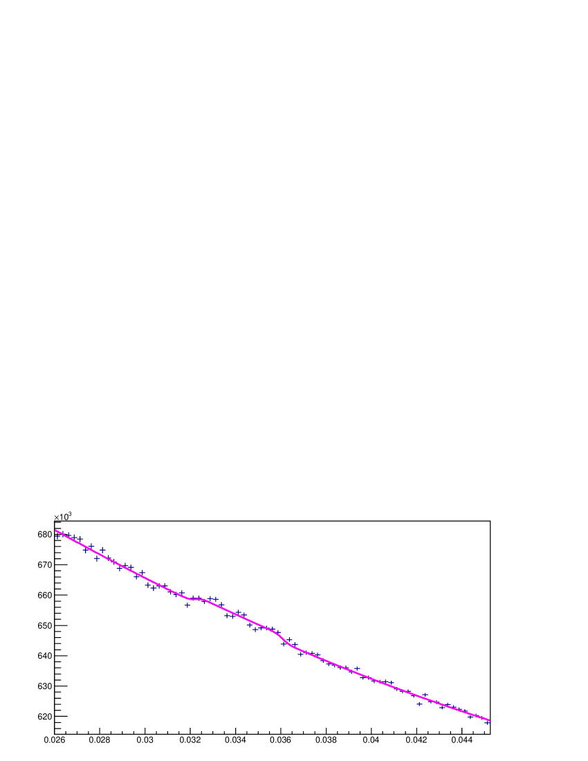
Figure 6: Fits to histograms of G-LG distances $d$, with $z$ in the range 0.25-0.45 for the northern galactic cap (N), that obtain $\hat{d}_{\alpha}$ at $z=0.36$. From top to bottom, they correspond to SDSS DR14 (this analysis), DR14 with galaxy selections of BH_ijaa , and DR13 with galaxy selections of BH_ijaa . The fits obtain $\hat{d}_{\alpha}=0.03455\pm 0.00010,0.03416\pm 0.00010,\textrm{ and }0.03431\pm 0.00012$ respectively, where uncertainties are statistical from the fits. Note that our assigned total uncertainty for $\hat{d}_{\alpha}$ is $\pm 0.00030$. This single fit for the current analysis, together with $\theta_{*}$ obtains $\Omega_{m}=0.272\pm 0.007$ and $d_{*}=0.0345\pm 0.0004$, with zero degrees of freedom. The relative amplitudes $A$ of the fitted signals are $0.00552\pm 0.00060,0.00369\pm 0.00042,\textrm{ and }0.00341\pm 0.00039$ respectively. The number of galaxies (G) and large galaxies (LG) are $(114597,65130)$, $(153783,101504)$, and $(160943,107971)$, respectively. Note that the relative amplitude is larger for the current galaxy selections.

Appendix A Comparison with Reference BH_ijaa

Tables 4 and 5 of Reference BH_ijaa can be compared with Tables 6 and 7 of the present analysis. We find agreement between all measurements when $d$ in Reference BH_ijaa is identified with $d_{*}$ in the present analysis. We find that $d$ in Table 4 of Reference BH_ijaa is biased low with respect to $d_{\textrm{\small{drag}}}$ in Table 6 of the present analysis. For the scenario of flat space and a cosmological constant, Table 4 of Reference BH_ijaa obtains $\Omega_{m}=0.284\pm 0.014$ and $d=0.0339\pm 0.0002$. From this $\Omega_{m}$ and Equation (4) we obtain $d_{*}=0.0338\pm 0.0007$, in good agreement with $d$, so in Reference BH_ijaa no correction for $d_{\textrm{\small{drag}}}/d_{*}$ was needed or applied.

Appendix B Bias of BAO measurements of small galaxy samples

We have investigated the difference of $d_{\textrm{\small{drag}}}$ between Reference BH_ijaa and the present analysis. This difference is not due to the change of data set from SDSS DR13 to SDSS DR14: we have compared the coordinates of selected galaxies and have found no changes in calibrations. The fluctuation is not caused by the tighter galaxy selection requirements of the present analysis: compare the entries with “&” and “$*$” in Table 1, and see Figure 6.

As a test, we divide the bin $0.425<z<0.725$ into 6 sub-samples: $0.425<z<0.525$ N, $0.525<z<0.625$ N, $0.625<z<0.725$ N, $0.425<z<0.525$ S, $0.525<z<0.625$ S, and $0.625<z<0.725$ S. We try to fit each one, and average the successful fits (only about half are successful), and obtain $\hat{d}_{\alpha}=0.03358\pm 0.00015$, $\hat{d}_{/}=0.03415\pm 0.00027$, and $\hat{d}_{z}=0.03335\pm 0.00033$. We also fit the sum of these six bins, and obtain $\hat{d}_{\alpha}=0.03496\pm 0.00015$, $\hat{d}_{/}=0.03459\pm 0.00010$, and $\hat{d}_{z}=0.03464\pm 0.00034$. So there is evidence that fits become biased low as the number of galaxies is reduced and the significance of the fitted relative amplitude $A$ of the BAO signal becomes marginal. The reason is that the observed BAO signal has a sharper and larger lower edge at $\approx 0.032$ compared to the upper edge at $\approx 0.037$, so the upper edge tends to get lost in the background fluctuations as the number of galaxies is reduced.

To reduce this bias, in the present analysis we require the significance of the fitted relative amplitudes $A/\sigma_{A}>2$, instead of $>1$ for Reference BH_ijaa . The price to pay is that we obtain only 2 independent bins of $z$, instead of 6.

Appendix C A study of the BAO signal

The BAO signal has a “step-up-step-down” shape with center at $\hat{d}$ and half-width $\Delta$. The widths of fits vary typically from $\Delta=0.0017$ to 0.0025, see Table 2. We have used the center $\hat{d}$ as the BAO standard ruler, but could have used the lower edge of the signal at $\hat{d}-\Delta$, or the upper edge at $\hat{d}+\Delta$, or somewhere in between, i.e. $\hat{d}+\epsilon\Delta$. We have investigated the value of $\epsilon$ that minimizes the root-mean-square fluctuations of a representative selection of measurements. The result is $\epsilon=-0.17$, and the difference in the r.m.s. values is negligible (0.00037 vs. 0.00039) so we keep the center of the signal as our standard ruler, i.e. $\epsilon=0$. The r.m.s. fluctuation of the lower edge with $\epsilon=-1$ is 0.00068, and the fluctuation of the upper edge with $\epsilon=1$ is 0.00091, which again illustrates the bias described in Appendix B, i.e. the lower edge fluctuates less than the upper edge.

A separate open question is whether this center $\hat{d}$ coincides with the $d_{\textrm{\small{drag}}}$ of Equation (5)?

Yet another question is this: what value of $\epsilon$ would reproduce the Planck $\Omega_{m}$? We obtain $\epsilon$ ranging from $-0.81$ for $\hat{d}_{\alpha}$ at $z=0.34$, to $\epsilon=-0.43$ for $\hat{d}_{z}$ at $z=0.56$. These large values of $|\epsilon|$, and their strong dependence on $z$ and galaxy-galaxy orientation, do not seem plausible.

Finally, how well do we understand $d_{\textrm{\small{drag}}}/d_{*}$? The present study takes $z_{\textrm{\small{drag}}}=1059.94\pm 0.30$ and $d_{\textrm{\small{drag}}}/d_{*}=1.0184\pm 0.0004$ from the Planck analysis Planck . Note the extremely small uncertainty obtained by the Planck Collaboration. In comparison, from Eq. (4) of Reference drag we obtain $z_{\textrm{\small{drag}}}=1020.82$ and $d_{\textrm{\small{drag}}}/d_{*}=1.044$.

An estimate of the uncertainties due to the issues discussed in these appendices is included in Table 5.

References

- (1) Hoeneisen, B. (2017) Study of Baryon Acoustic Oscillations with SDSS DR13 Data and Measurements of and . International Journal of Astronomy and Astrophysics, 7, 11-27. https://doi.org/10.4236/ijaa.2017.71002
- (2) Review of Particle Physics, C. Patrignani et al. (Particle Data Group), Chin. Phys. C, 40, 100001 (2016)
- (3) Planck Collaboration: N. Aghanim et al. , Planck 2018 results. VI. Cosmological parameters, arXiv:1807.06209 (2018)
- (4) The Review of Particle Physics (2018), M. Tanabashi et al. (Particle Data Group), Phys. Rev. D 98, 030001 (2018).
-
(5)
Hoeneisen, B.
(2018) Study of Galaxy Distributions with SDSS DR14
Data and Measurement of Neutrino Masses.
International Journal of Astronomy and
Astrophysics, 8, 230-257.
https://doi.org/10.4236/ijaa.2018.83017 - (6) Blanton, M.R. et al., Sloan Digital Sky Survey IV: Mapping the Milky Way, Nearby Galaxies, and the Distant Universe, The Astronomical Journal, Volume 154, Issue 1, article id. 28, 35 pp. (2017)
- (7) Dawson, K.S., et al., The Baryon Oscillation Spectroscopic Survey of SDSS-III, The Astronomical Journal, Volume 145, Issue 1, article id. 10, 41 pp. (2013)
- (8) D. J. Eisenstein, H.-J. Seo, and M. White, On the Robustness of the Acoustic Scale in the Low-Redshift Clustering of Matter, ApJ, 664: 660-674 (2007)
- (9) Hoeneisen, B. (2000) A simple model of the hierarchical formation of galaxies. arXiv:astro-ph/0009071
- (10) Steven Weinberg, Cosmology, Oxford University Press (2008)
- (11) Hee-Jong Seo, et al., High-precision predictions for the acoustic scale in the non-linear regime, ApJ, 720, 1650 (2010).
- (12) M. Chevallier, D. Polarski, Accelerating Universes with Scaling Dark Matter, Int. J. Mod. Phys. D10, 213 (2001)
- (13) Eric V. Linder, Exploring the Expansion History of the Universe, Phys.Rev.Lett. 90:091301 (2003)
- (14) Andreu Font-Ribera et al., Quasar-Lyman α forest cross-correlation from BOSS DR11: Baryon Acoustic Oscillations, J. Cosmology Astropart. Phys. 05, 027 (2014), arXiv:1311.1767.
- (15) Timothée Delubac, et al., Baryon Acoustic Oscillations in the Ly forest of BOSS DR11 quasars, arXiv:1404.1801v2 (2014).
- (16) Riess, A. G., Casertano, S., Yuan, W., et al. (2018), New Parallaxes of Galactic Cepheids from Spatially Scanning the Hubble Space Telescope: Implications for the Hubble Constant, ApJ, 861, 126. arXiv:1801.01120
- (17) A. Vikhlinin et al., Chandra Cluster Cosmology Project III: Cosmological Parameter Constraints, Astrophys. J. 692, 1060 (2009).
- (18) H. Hildebrandt et al., KiDS-450: cosmological parameter constraints from tomographic weak gravitational lensing, Mon. Not. R. Astron. Soc 465, 1454 (2017).
- (19) Lesgourgues J., and Pastor S., Massive neutrinos and cosmology; Phys. Rep. 429 (2006) 307
- (20) Daniel J. Eisenstein and Wayne Hu, Baryonic Features in the Matter Transfer Function, arXiv:astro-ph/9709112 (1997)