An Unconditionally Energy-Stable Scheme Based on an Implicit Auxiliary Energy Variable for Incompressible Two-Phase Flows with Different Densities Involving Only Precomputable Coefficient Matrices

Abstract

We present an energy-stable scheme for numerically approximating the governing equations for incompressible two-phase flows with different densities and dynamic viscosities for the two fluids. The proposed scheme employs a scalar-valued auxiliary energy variable in its formulation, and it satisfies a discrete energy stability property. More importantly, the scheme is computationally efficient. Within each time step, it computes two copies of the flow variables (velocity, pressure, phase field function) by solving individually a linear algebraic system involving a constant and time-independent coefficient matrix for each of these field variables. The coefficient matrices involved in these linear systems only need to be computed once and can be pre-computed. Additionally, within each time step the scheme requires the solution of a nonlinear algebraic equation about a scalar-valued number using the Newton’s method. The cost for this nonlinear solver is very low, accounting for only a few percent of the total computation time per time step, because this nonlinear equation is about a scalar number, not a field function. Extensive numerical experiments have been presented for several two-phase flow problems involving large density ratios and large viscosity ratios. Comparisons with theory show that the proposed method produces physically accurate results. Simulations with large time step sizes demonstrate the stability of computations and verify the robustness of the proposed method. An implication of this work is that energy-stable schemes for two-phase problems can also become computationally efficient and competitive, eliminating the need for expensive re-computations of coefficient matrices, even at large density ratios and viscosity ratios.

Keywords: auxiliary variable; Implicit scalar auxiliary variable; energy stability; phase field; multiphase flows; two-phase flows

1 Introduction

This work concerns the simulation of the dynamics of a mixture of two immiscible incompressible fluids with possibly very different densities and dynamic viscosities based on the phase field approach. The presence of fluid interfaces, the associated surface tension, the density contrast and viscosity contrast play an important role in the dynamics of such systems, and these factors also make such numerical simulations very challenging. Phase field (or diffuse interface) Rayleigh1892 ; Waals1893 ; AndersonMW1998 ; LowengrubT1998 ; Jacqmin1999 ; LiuS2003 is one of the main approaches for dealing with fluid interfaces in the modeling of two-phase systems, along with other related methods OsherS1988 ; ScardovelliZ1999 ; Tryggvasonetal2001 ; SethianS2003 . It has attracted an increasing interest from the community in the past years, in part because of its physics-based nature. With this approach the fluid interface is treated to be diffuse, as a thin smooth transition layer AndersonMW1998 . The state of the system is characterized by, apart from the hydrodynamic variables such as velocity and pressure, an order parameter (or phase field variable), which varies smoothly within the transition layer and is mostly uniform in the bulk phases. The evolution of the system is characterized by, apart from the kinetic energy, a free energy density function, which contains component terms that promote the mixing of the two fluids and also component terms that tend to separate these fluids. The interplay of these two opposing tendencies determines the dynamic profile of the interface. The adoption of the free energy in the formulation makes it possible to relate to other thermodynamic variables. Indeed, with the phase field approach the governing equations of the system can be rigorously derived based on the conservation laws and thermodynamic principles. Several thermodynamically consistent phase field models are already available in the literature for two-phase and multiphase flows, see e.g. LowengrubT1998 ; KimL2005 ; AbelsGG2012 ; ShenYW2013 ; AkiDG2014 ; Dong2014 ; LiuSY2015 ; GongZW2017 ; Dong2018 ; RoudbariSBZ2018 , with various degrees of sophistication or the observance/violation of other physical principles such as Galilean invariance and reduction consistency. The mass conservation of the individual fluid components in the system, and the choice of an appropriate form for the free energy density function, naturally give rise to the Cahn-Hilliard equation in two phases or a system of coupled Cahn-Hilliard type equations (see e.g. AbelsGG2012 ; Dong2018 , among others).

We focus on the numerical approximation and simulation of the governing equations for incompressible two-phase flows with different densities and viscosities in this work. A computational scientist/engineer interested in such problems confronts a compromise and needs to balance two seemingly incompatible aspects: the desire to be able to use a larger time step size (permissible by accuracy), and the computational cost. On the one hand, semi-implicit splitting type schemes (see e.g. DongS2012 ; BadalassiCB2003 ; DingSS2007 ; Dong2012 ; Dong2014obc , among others) induces a very low computational cost per time step, because among other things only de-coupled linear algebraic systems need to be solved after discretization and these linear systems only involve constant and time-independent coefficient matrices that can be pre-computed (see DongS2012 ), even with large density ratios and viscosity ratios. The downside of these schemes lies in that they are only conditionally stable and the time step size is restricted by CFL or related conditions. On the other hand, energy-stable schemes (see e.g. ShenY2010 ; Salgado2013 ; GuoLL2014 ; GrunK2014 ; ShenY2015 ; GuoLLW2017 ; YuY2017 ; RoudbariSBZ2018 , among others) can potentially allow the use of much larger time step sizes in dynamic simulations. The downside lies in that, the computational cost per time step of these schemes can be very high. Energy-stable schemes often require the solution of coupled nonlinear algebraic field equations or coupled linear algebraic equations. The linear algebraic systems associated with these schemes involve time-dependent coefficient matrices, which require frequent re-computations (or at every time step).

Mindful of the strengths and weaknesses of both types of schemes, we would like to consider the following question. Can we devise an algorithm to combine the strengths of both types of schemes that can achieve unconditional energy stability and simultaneously require a relatively low computational cost? Summarized in this paper is our attempt to tackle this question and a numerical scheme that largely achieves this goal.

The current work has drawn inspirations from several previous studies in the literature. In the following we restrict our review of literature to the energy-stable schemes for the hydrodynamic interactions of two-phase flows with different densities and viscosities based on the phase field framework. This will leave out those algorithms that are devoted purely to the phase field such as the Cahn-Hilliard or Allen-Cahn equations CahnH1958 ; AllenC1979 without hydrodynamic interactions, for which a large volume of literature exists. Those studies considering only matched densities for the two fluids (see e.g. AlandC2016 ; HanBYT2017 ; YangY2018 , among others) will also be largely left out. In ShenY2010 a phase field model based on the combined Navier-Stokes/Allen-Cahn equations with different densities/viscosities for the two fluids is considered, and several discretely energy-stable schemes of first order in time are introduced based on projection, Gauge-Uzawa, and pressure stabilization formulations. What is interesting lies in that all these schemes are linear in nature. They only require the solution of linear, albeit coupled, algebraic equations for different flow variables after discretization. To accommodate different densities for the two fluids, the authors of ShenY2010 have adopted a reformulation of the inertial term GuermondQ2000 in the Navier-Stokes equation, which as pointed out by GrunK2014 might not be consistent with the phase field equation employed therein. Corresponding schemes for a Navier-Stokes/Cahn-Hilliard model are presented in ShenY2010cam . A fractional-step scheme based on a pressure correction-type strategy is developed in Salgado2013 for a phase-field model in which the chemical potential contains a velocity term (see also LiuSY2015 ), together with a generalized Navier type boundary condition for contact lines QianWS2006 . This scheme is linear, and the discrete equations about the phase field function and the velocity are coupled together. Improved algorithms for the Navier-Stokes/Cahn-Hilliard model are later developed by ShenY2015 , in which the discrete phase field equation and the momentum equations are de-coupled thanks to an extra stabilization term BoyerM2011 employed for approximating the convection velocity in the Cahn-Hilliard equation. The scheme is first order in time, and it is unclear whether an analogous second-order stabilization term exists for the approximation of the convection velocity. In GrunK2014 a discretely energy stable scheme for the phase field model of AbelsGG2012 is developed, which gives rise to a system of nonlinear algebraic equations that couple together all the flow variables. It is interesting to note that the algorithm developed in YuY2017 for the same phase field model only requires the solution of linear equations and that the phase-field and momentum equations are de-coupled owing to the same treatment of the discrete convection velocity of the Cahn-Hilliard equation as in ShenY2015 . Two discretely energy stable schemes are described in GuoLL2014 ; GuoLLW2017 for the quasi-incompressible Navier-Stokes/Cahn-Hilliard model of LowengrubT1998 . The schemes can preserve the mass conservation on the discrete level, and they lead to coupled highly-nonlinear algebraic systems after discretization. Numerical schemes for related quasi-incompressible hydrodynamic phase field models have also been proposed in GongZW2017 ; RoudbariSBZ2018 ; GongZYW2018 . In particular, in GongZYW2018 the so-called invariant energy quadratization method has been used to reformulate the phase field equation, and the resultant numerical schemes are second-order in time, and involve the solution of linear algebraic systems that couple together the different flow variables.

Apart from the many contributions discussed above, an interesting strategy for formulating energy-stable schemes for gradient-type dynamical systems (gradient flows) based on certain auxiliary variables has emerged recently Yang2016 ; ShenXY2018 . The invariant energy quadratization (IEQ) method Yang2016 introduces an auxiliary field function related to the square root of the potential free energy density function together with a dynamic equation for this auxiliary variable, and allows one to reformulate the gradient-flow evolution equation to facilitate schemes for ensuring the energy stability relatively easily. The scalar auxiliary variable (SAV) method ShenXY2018 introduces an auxiliary variable, which is a scalar-valued number rather than a field function, related to the square root of the total potential energy integral, and a dynamic equation about this scalar variable. Both types of auxiliary variables can simplify the formulation of schemes to achieve energy stability for gradient flows.

Another recent development that inspires the current work is LinD2018 , in which an energy-stable scheme for the incompressible Navier-Stokes equations based on a scalar auxiliary variable related to the total kinetic energy has been developed. Because the Navier-Stokes equation is not a gradient-type system, the scalar auxiliary variable formulation as developed in ShenXY2018 for gradient flows cannot be directly used. Indeed, it is observed that if one reformulates the viscous term in the Navier-Stokes equation using the auxiliary variable, in a way analogous to the treatment of the dissipation term in the evolution equation for gradient flows, the simulation results turn out to be very poor. Instead, a viable strategy for Navier-Stokes equations seems to be to control the convection term with the auxiliary variable. Such a strategy is presented in LinD2018 , which hinges on reformulating the convection-term contribution into a boundary integral in the dynamic equation for the auxiliary total kinetic energy.

In this paper we build upon the scalar auxiliary variable idea and present an energy-stable scheme for the numerical approximation of the two-phase governing equations with different densities and viscosities for the two fluids based on the phase field model of AbelsGG2012 . By introducing a scalar-valued variable related to the total of the kinetic energy and the potential free energy of the two-phase system, we reformulate the two-phase governing equations into an equivalent form. By carefully treating the variable-density and variable-viscosity terms, we show that the proposed scheme honors a discrete energy stability relation. We present an efficient solution algorithm and a procedure for dealing with the integrals of the unknown field functions. Within each time step, our algorithm only requires the solution of several de-coupled individual linear algebraic systems, each for an individual field function, together with the solution of a nonlinear algebraic equation about a scalar-valued number. More importantly, those linear algebraic systems to be solved within a time step each involves a constant and time-independent coefficient matrix, which only needs to be computed once and can be pre-computed. The nonlinear algebraic equation involved therein requires Newton iterations in its solution. But its computational cost is very low, because this equation is about a single scalar number, not a field function. Numerical experiments show that the solution for the nonlinear equation accounts for around $8\%$ of the total solver time within a time step, and essentially all this time is spent on computing the coefficients involved in the nonlinear equation in preparation for the Newton method, rather than in the actual Newton iterations. Because of these attractive properties, our algorithm is computationally very efficient. We will present a number of numerical experiments to demonstrate the stability of our method at large time step sizes for two-phase problems.

The new aspects of this work include the following: (i) the energy-stable scheme for the two-phase governing equations with different densities and viscosities for the two fluids, and (ii) the efficient solution algorithm for implementing the proposed scheme. The property of our solution algorithm that it involves only linear algebraic systems with constant and time-independent coefficient matrices, even at large density ratios and viscosity ratios, is particular attractive, because this makes the cost low and the method computationally very efficient. To the best of the authors’ knowledge, this is the first energy-stable scheme which involves only constant and time-independent coefficient matrices for incompressible two-phase flows with different densities and viscosities for the two fluids.

The rest of this paper is organized as follows. In Section 2, we introduce a scalar-valued auxiliary variable and reformulate the two-phase governing equations into an equivalent system employing this variable. Then we present a scheme for temporal discretization for the reformulated equivalent system, and prove that the scheme satisfies a discrete energy law. An efficient solution algorithm for implementing the scheme will be presented, and the spatial discretization based on $C^{0}$ spectral elements will be discussed. In Section 3 we present a few numerical examples of two-phase flows involving large density ratios and viscosity ratios to demonstrate the accuracy of our method and also its stability at large time step sizes. Section 4 then concludes the discussions with some closing remarks.

2 Energy-Stable Scheme for Incompressible Two-Phase Flows

2.1 Governing Equations

Consider a mixture of two immiscible incompressible fluids contained in some domain $\Omega$ in two or three dimensions, whose boundary is denoted by $\partial\Omega$. Let $\rho_{1}$ and $\rho_{2}$ respectively denote the constant densities of the two fluids, and $\mu_{1}$ and $\mu_{2}$ denote their constant dynamic viscosities. The conservations of mass/momentum and the second law of thermodynamics for this two-phase system lead to the following coupled system of equations (see e.g. AbelsGG2012 ; Dong2014 for details):

$$\rho\frac{D\bm{u}}{Dt}+\tilde{\bm{J}}\cdot\nabla\bm{u}=-\nabla p+\nabla\cdot[\mu\mathcal{\bm{D}}(\bm{u})]-\lambda\nabla\cdot(\nabla\phi\nabla\phi)+\bm{f}(\bm{x},t),$$ (1a)

$$\nabla\cdot\bm{u}=0,$$ (1b)

$$\frac{D\phi}{Dt}=m\nabla^{2}\mathcal{C}+g(\bm{x},t),$$ (1c)

$$\mathcal{C}=-\lambda\nabla^{2}\phi+h(\phi),$$ (1d)

where $\frac{D}{Dt}=\frac{\partial}{\partial t}+\bm{u}\cdot\nabla$ is the material derivative, and $\mathcal{\bm{D}}(\bm{u})=\nabla\bm{u}+\nabla\bm{u}^{T}.$ In the above equations, $\bm{u}(\bm{x},t)$ is the velocity, $p(\bm{x},t)$ is the pressure, and $\bm{f}(\bm{x},t)$ is an external body force, where $t$ is time and $\bm{x}$ is the spatial coordinate and $(\cdot)^{T}$ denotes the transpose of $(\cdot).$ $\phi(\bm{x},t)$ denotes the phase field function, $-1\leq\phi\leq 1.$ The flow regions with $\phi=1$ and $\phi=-1$ respectively represent the first and the second fluids. The iso-surface $\phi(\bm{x},t)=0$ marks the interface between the two fluids at time $t.$ The function $h(\phi)$ in equation (1d) is given by

$$h(\phi)=F^{\prime}(\phi)=\frac{\lambda}{\eta^{2}}\phi(\phi^{2}-1)\;\;\text{with}\;\;F(\phi)=\frac{\lambda}{4\eta^{2}}(1-\phi^{2})^{2},$$ (2)

where $\eta$ is a characteristic length scale of the interface thickness, and $F(\phi)$ is the potential free energy density (double-well function) of the system. $\mathcal{C}$ in the above equations denotes the chemical potential, satisfying the relation $\mathcal{C}=\frac{\delta W}{\delta\phi},$ where $W$ is the free energy of the system given by $W=\int_{\Omega}\left[\frac{\lambda}{2}\nabla\phi\cdot\nabla\phi+F(\phi)\right].$ $\lambda$ is the mixing energy density coefficient and is related to the surface tension by YueFLS2004

$$\lambda=\frac{3}{2\sqrt{2}}\sigma\eta,$$ (3)

where $\sigma$ is the interface surface tension and is assumed to be a constant. $m>0$ is the mobility of the interface, and is assumed to be a constant in the current paper. The density $\rho$ and the dynamic viscosity $\mu$ of the two-phase mixture are related to the phase field function by

$$\rho(\phi)=\frac{\rho_{1}+\rho_{2}}{2}+\frac{\rho_{1}-\rho_{2}}{2}\phi,\quad\mu(\phi)=\frac{\mu_{1}+\mu_{2}}{2}+\frac{\mu_{1}-\mu_{2}}{2}\phi.$$ (4)

In equation (1a), $\tilde{\bm{J}}$ is given by

$$\tilde{\bm{J}}(\phi)=J_{0}\nabla\mathcal{C}=J_{0}\nabla\big{(}-\lambda\nabla^{2}\phi+h(\phi)\big{)},\quad{\rm with}\;\;J_{0}=-\frac{1}{2}(\rho_{1}-\rho_{2})m.$$ (5)

Note that $\tilde{\bm{J}}$ and $\rho$ given above satisfy the following relation

$$\frac{D\rho}{Dt}=-\nabla\cdot\tilde{\bm{J}}.$$ (6)

$g(\bm{x},t)$ in equation (1c) is a prescribed source term for the purpose of numerical testing only, and will be set to $g=0$ in actual simulations.

To facilitate subsequent development of the unconditionally energy-stable scheme, we transform equation (1a) into an equivalent form:

$$\rho\frac{D\bm{u}}{Dt}+\tilde{\bm{J}}\cdot\nabla\bm{u}=-\nabla P+\nabla\cdot[\mu\mathcal{\bm{D}}(\bm{u})]+\mathcal{C}\nabla\phi+\bm{f}(\bm{x},t),$$ (7)

where $P=p+\frac{\lambda}{2}\nabla\phi\cdot\nabla\phi+F(\phi)$ is an effective pressure and we have used the following identity

$$\nabla\cdot(\nabla\phi\nabla\phi)=\frac{1}{2}\nabla(\nabla\phi\cdot\nabla\phi)+(\nabla^{2}\phi)\nabla\phi.$$

It can be shown that the system consisting of equations (1a)–(1d), with $\bm{f}=0$ and $g=0$, satisfies the following energy law (assuming that all boundary flux terms vanish),

$$\frac{d}{dt}\int_{\Omega}\left[\frac{1}{2}\rho|\bm{u}|^{2}+\frac{\lambda}{2}\nabla\phi\cdot\nabla\phi+F(\phi)\right]=-\int_{\Omega}\frac{\mu}{2}\left\|\nabla\bm{u}\right\|^{2}-\int_{\Omega}m\nabla\mathcal{C}\cdot\nabla\mathcal{C}.$$ (8)

Equations (7), (1b)-(1d) are to be supplemented by appropriate boundary and initial conditions for the velocity and the phase field function. We assume the following boundary conditions:

$$\bm{u}|_{\partial\Omega}=\bm{w}(\bm{x},t),$$ (9)

$$\bm{n}\cdot\nabla\phi|_{\partial\Omega}=d_{a}(\bm{x},t),$$ (10)

$$\bm{n}\cdot\nabla(\nabla^{2}\phi)|_{\partial\Omega}=d_{b}(\bm{x},t),$$ (11)

and the initial conditions:

$$\bm{u}(\bm{x},0)=\bm{u}_{in}(\bm{x}),$$ (12)

$$\phi(\bm{x},0)=\phi_{in}(\bm{x}).$$ (13)

In the above equations $d_{a}$ and $d_{b}$ are prescribed source terms for the purpose of numerical testing only, and will be set to $d_{a}=0$ and $d_{b}=0$ in actual simulations. The boundary conditions (10) and (11) with $d_{a}=0$ and $d_{b}=0$ correspond to a solid-wall boundary of neutral wettability, i.e. contact angle is $90^{0}$ when the fluid interface intersects the wall. $\bm{u}_{in}(\bm{x})$ and $\phi_{in}(\bm{x})$ are the initial velocity and phase field distributions.

2.2 Reformulated Equivalent System of Equations

To derive the energy-stable scheme for the system (7), (1b)-(1d), we introduce a shifted energy consisting of the kinetic energy and the potential free energy component as follows,

$$E(t)=\int_{\Omega}\Big{[}\frac{1}{2}\rho|\bm{u}|^{2}+F(\phi)\Big{]}d\Omega+C_{0}$$ (14)

where $C_{0}$ is a chosen constant such that $E(t)>0$ for all $t\geq 0.$ Note that $E(t)$ is a scalar-valued number, not a field function. Define an auxiliary variable

$$R(t)=\sqrt{E(t)}.$$ (15)

With the help of the identities

$$\left\{\begin{split}&\rho\frac{D\bm{u}}{Dt}\cdot\bm{u}=\frac{D}{Dt}\Big{(}\frac{1}{2}\rho|\bm{u}|^{2}\Big{)}-\frac{D\rho}{Dt}\Big{(}\frac{1}{2}|\bm{u}|^{2}\Big{)}\\ &\Big{(}\tilde{\bm{J}}\cdot\nabla\bm{u}\Big{)}\cdot\bm{u}=\nabla\cdot\Big{(}\frac{1}{2}|\bm{u}|^{2}\tilde{\bm{J}}\Big{)}-\nabla\cdot\tilde{\bm{J}}\Big{(}\frac{1}{2}|\bm{u}|^{2}\Big{)}\\ &\bm{u}\cdot\nabla\Big{(}\frac{1}{2}\rho|\bm{u}|^{2}\Big{)}=\nabla\cdot\Big{(}\frac{1}{2}\rho|\bm{u}|^{2}\bm{u}\Big{)}-(\nabla\cdot\bm{u})\frac{1}{2}\rho|\bm{u}|^{2}\end{split}\right.$$ (16)

and the equations (1b) and (6), we can obtain that

$$\frac{\partial}{\partial t}\Big{(}\frac{1}{2}\rho|\bm{u}|^{2}\Big{)}=\rho\frac{D\bm{u}}{Dt}\cdot\bm{u}+\Big{(}\tilde{\bm{J}}\cdot\nabla\bm{u}\Big{)}\cdot\bm{u}-\nabla\cdot\Big{(}\frac{1}{2}\tilde{\bm{J}}|\bm{u}|^{2}\Big{)}-\nabla\cdot\Big{(}\frac{1}{2}\rho|\bm{u}|^{2}\bm{u}\Big{)}.$$ (17)

Thus, taking the derivative of $R(t)$ leads to

$$\begin{split}2R\frac{dR}{dt}&=\frac{dE}{dt}=\int_{\Omega}\frac{\partial}{\partial t}\Big{[}\frac{1}{2}\rho|\bm{u}|^{2}+F(\phi)\Big{]}\\ &=\int_{\Omega}\Big{[}\rho\Big{(}\frac{\partial\bm{u}}{\partial t}+\bm{u}\cdot\nabla\bm{u}\Big{)}+\tilde{\bm{J}}\cdot\nabla\bm{u}\Big{]}\cdot\bm{u}+\int_{\Omega}h(\phi)\frac{\partial\phi}{\partial t}-\int_{\partial\Omega}(\bm{n}\cdot\bm{u})\frac{1}{2}\rho|\bm{u}|^{2}-\int_{\partial\Omega}\Big{(}\bm{n}\cdot\tilde{\bm{J}}\Big{)}\frac{1}{2}|\bm{u}|^{2},\end{split}$$ (18)

where $\bm{n}$ is the outward-pointing unit vector normal to the boundary $\partial\Omega,$ and we have used equation (17), integration by part, and the divergence theorem. It is crucial to note that both $E(t)$ and $R(t)$ are scalar-valued variables depending only on $t$, and the fact that

$$\frac{R(t)}{\sqrt{E(t)}}=1.$$ (19)

In light of equation (19), we can re-write the system consisting of equations (7), (1b)-(1d) into the following equivalent form

$$\begin{split}\rho\frac{\partial\bm{u}}{\partial t}+\frac{R(t)}{\sqrt{E(t)}}\Big{\{}\rho\bm{u}\cdot\nabla\bm{u}+&\tilde{\bm{J}}\cdot\nabla\bm{u}-\nabla\mu\cdot\mathcal{\bm{D}}(\bm{u})+\Big{(}1-\frac{\rho}{\rho_{0}}\Big{)}\nabla P+(\mu-\nu_{m}\rho)\nabla\times\nabla\times\bm{u}\Big{\}}\\ &=-\frac{\rho}{\rho_{0}}\nabla P+\nu_{m}\rho\nabla^{2}\bm{u}+\mathcal{C}\nabla\phi+\bm{f},\end{split}$$ (20)

$$\nabla\cdot\bm{u}=0,$$ (21)

$$\frac{\partial\phi}{\partial t}+\frac{R(t)}{\sqrt{E(t)}}\bm{u}\cdot\nabla\phi=m\nabla^{2}\mathcal{C}+g,$$ (22)

$$\mathcal{C}=-\lambda\nabla^{2}\phi+S\Big{(}\phi-\phi\Big{)}+\frac{R(t)}{\sqrt{E(t)}}h(\phi),$$ (23)

$$\begin{split}2R\frac{dR}{dt}&=\int_{\Omega}\rho\frac{\partial\bm{u}}{\partial t}\cdot\bm{u}-\int_{\Omega}\mathcal{C}\nabla\phi\cdot\bm{u}+\frac{R(t)}{\sqrt{E(t)}}\int_{\Omega}\mathcal{C}\nabla\phi\cdot\bm{u}+\frac{R(t)}{\sqrt{E(t)}}\int_{\Omega}h(\phi)\frac{\partial\phi}{\partial t}\\ &+\frac{R(t)}{\sqrt{E(t)}}\int_{\Omega}\Big{\{}\rho\bm{u}\cdot\nabla\bm{u}+\tilde{\bm{J}}\cdot\nabla\bm{u}-\nabla\mu\cdot\mathcal{\bm{D}}(\bm{u})+\Big{(}1-\frac{\rho}{\rho_{0}}\Big{)}\nabla P+(\mu-\nu_{m}\rho)\nabla\times\nabla\times\bm{u}\Big{\}}\cdot\bm{u}\\ &+\int_{\Omega}\Big{\{}\nabla\cdot\left[\mu\mathcal{\bm{D}}(\bm{u})\right]+\Big{(}\frac{\rho}{\rho_{0}}-1\Big{)}\nabla P-\nu_{m}\rho\nabla^{2}\bm{u}\Big{\}}\cdot\bm{u}\\ &-\frac{1}{2}\int_{\partial\Omega}(\bm{n}\cdot\bm{u})\rho|\bm{u}|^{2}-\frac{1}{2}\int_{\partial\Omega}\Big{(}\bm{n}\cdot\tilde{\bm{J}}\Big{)}|\bm{u}|^{2}.\end{split}$$ (24)

To obtain equations (20) and (24), we have used equation (1b) and the identities

$$\left\{\begin{split}&\nabla\cdot[\mu\mathcal{D}(\bm{u})]=\mu[\nabla^{2}\bm{u}+\nabla(\nabla\cdot\bm{u})]+\nabla\mu\cdot\mathcal{D}(\bm{u}),\\ &\nabla^{2}\bm{u}=\nabla(\nabla\cdot\bm{u})-\nabla\times\nabla\times\bm{u},\end{split}\right.$$

and have added/subtracted appropriate terms such as $\frac{\rho}{\rho_{0}}\nabla P$, $\nu_{m}\rho\nabla^{2}\bm{u}$, $S\phi$, and $\mathcal{C}\nabla\phi\cdot\bm{u}$. In these equations, $\rho_{0}$ is a constant given by $\rho_{0}={\rm min}(\rho_{1},\rho_{2}),$ $\nu_{m}$ is a chosen constant satisfying $\nu_{m}\geq\frac{1}{2}\max\left(\frac{\mu_{1}}{\rho_{1}},\frac{\mu_{2}}{\rho_{2}}\right),$ and $S$ is a chosen constant satisfying a condition to be specified later in equation (57).

The original system consisting of equations (7), (1b)-(1d), (9)-(13) is equivalent to the reformulated system consisting of equations (20)-(24), together with the boundary conditions (9)-(11), and the initial conditions (12)-(13), supplemented by an extra initial condition for $R(t),$ i.e.

$$R(0)=\Big{(}\int_{\Omega}\Big{[}\frac{1}{2}\rho(\phi_{in})|\bm{u}_{in}|^{2}+F(\phi_{in})\Big{]}d\Omega+C_{0}\Big{)}^{1/2}.$$ (25)

In the reformulated system, the dynamic variables are $\bm{u}(\bm{x},t)$, $P(\bm{x},t)$, $\phi(\bm{x},t)$ and $R(t)$. Note that $E(t)$ is computed by equation (14). We next focus on this reformulated equivalent system of equations, and present an unconditionally energy-stable scheme for approximating this system.

2.3 Formulation of Numerical Scheme

Let $n\geq 0$ denote the time step index, and $(\cdot)^{n}$ denote the variable $(\cdot)$ at time step $n.$ Let $J\;(J=1\;\text{or}\;2)$ denote the temporal order of accuracy of the scheme. We set

$$\phi^{0}=\phi_{in},\quad\bm{u}^{0}=\bm{u}_{in},\quad R^{0}=R(0),$$ (26)

where $R(0)$ is given in equation (25). Define a scalar-valued variable $\xi^{n+1}$

$$\xi^{n+1}=\frac{R^{n+1}}{\sqrt{E^{n+1}}}.$$ (27)

Given $(\phi,\bm{u},P,R)$ at time step $n$ and previous time steps, we compute $(\phi^{n+1},\bm{u}^{n+1},P^{n+1},R^{n+1})$ through the following scheme

$$\begin{split}\bar{\rho}^{n+1}\Big{(}\frac{\gamma_{0}\bm{u}^{n+1}-\hat{\bm{u}}}{\Delta t}\Big{)}&+\xi^{n+1}\bar{\rho}^{n+1}\bm{\mathcal{N}}=\\ &-\frac{\bar{\rho}^{n+1}}{\rho_{0}}\nabla P^{n+1}+\nu_{m}\bar{\rho}^{n+1}\nabla^{2}\bm{u}^{n+1}+\mathcal{C}^{n+1}\nabla\bar{\phi}^{n+1}+\bm{f}^{n+1},\end{split}$$ (28)

$$\nabla\cdot\bm{u}^{n+1}=0,$$ (29)

$$\frac{\gamma_{0}\phi^{n+1}-\hat{\phi}}{\Delta t}+\xi^{n+1}\big{(}\bm{u}^{*,n+1}\cdot\nabla\phi^{*,n+1}\big{)}=m\nabla^{2}\mathcal{C}^{n+1}+g^{n+1},$$ (30)

$$\mathcal{C}^{n+1}=-\lambda\nabla^{2}\phi^{n+1}+S\big{(}\phi^{n+1}-\phi^{*,n+1}\big{)}+\xi^{n+1}h(\phi^{*,n+1}),$$ (31)

$$\begin{split}&2R^{n+1}\frac{\gamma_{0}R^{n+1}-\hat{R}}{\Delta t}=\int_{\Omega}\bar{\rho}^{n+1}\Big{(}\frac{\gamma_{0}\bm{u}^{n+1}-\hat{\bm{u}}}{\Delta t}\Big{)}\cdot\bm{u}^{n+1}-\int_{\Omega}\mathcal{C}^{n+1}\big{(}\bm{u}^{n+1}\cdot\nabla\bar{\phi}^{n+1}\big{)}\\ &+\xi^{n+1}\int_{\Omega}\mathcal{C}^{n+1}\big{(}\bm{u}^{*,n+1}\cdot\nabla\phi^{*,n+1}\big{)}+\xi^{n+1}\int_{\Omega}h(\phi^{*,n+1})\frac{\gamma_{0}\phi^{n+1}-\hat{\phi}}{\Delta t}+\xi^{n+1}\int_{\Omega}\bar{\rho}^{n+1}\bm{\mathcal{N}}\cdot\bm{u}^{n+1}\\ &+\int_{\Omega}\Big{\{}\nabla\bar{\mu}^{n+1}\cdot\mathcal{\bm{D}}(\bm{u}^{n+1})+\Big{(}\frac{\bar{\rho}^{n+1}}{\rho_{0}}-1\Big{)}\nabla P^{n+1}+(\bar{\mu}^{n+1}-\nu_{m}\bar{\rho}^{n+1})\nabla^{2}\bm{u}^{n+1}\Big{\}}\cdot\bm{u}^{n+1}\\ &-\frac{1}{2}\int_{\partial\Omega}(\bm{n}\cdot\bm{u}^{n+1})\bar{\rho}^{n+1}\big{|}\bm{u}^{n+1}\big{|}^{2}-\frac{1}{2}\int_{\partial\Omega}\Big{(}\bm{n}\cdot\tilde{\bm{J}}^{n+1}\Big{)}\big{|}\bm{u}^{n+1}\big{|}^{2},\end{split}$$ (32)

$$\bm{u}^{n+1}=\bm{w}^{n+1}\;\;\;{\rm on}\;\;\partial\Omega,$$ (33)

$$\bm{n}\cdot\nabla\phi^{n+1}=d_{a}^{n+1}\;\;\;{\rm on}\;\;\partial\Omega$$ (34)

$$\bm{n}\cdot\nabla(\nabla^{2}\phi^{n+1})=d_{b}^{n+1}\;\;\;{\rm on}\;\;\partial\Omega.$$ (35)

The symbols in the above equations are defined as follows. In equations (28) and (32)

$$\bm{\mathcal{N}}={\bm{{Q}}}+\Big{(}\frac{\bar{\mu}^{n+1}}{\bar{\rho}^{n+1}}-\nu_{m}\Big{)}\nabla\times\nabla\times\bm{u}^{*,n+1},$$ (36)

and

$$\begin{split}{\bm{{Q}}}={\bm{{Q}}}(\bar{\phi}^{n+1},\bm{u}^{*,n+1})&=\bm{u}^{*,n+1}\cdot\nabla\bm{u}^{*,n+1}+\frac{1}{\bar{\rho}^{n+1}}\bar{\tilde{\bm{J}}}^{n+1}\cdot\nabla\bm{u}^{*,n+1}-\frac{1}{\bar{\rho}^{n+1}}\nabla\bar{\mu}^{n+1}\cdot\mathcal{\bm{D}}(\bm{u}^{*,n+1})\\ &+\Big{(}\frac{1}{\bar{\rho}^{n+1}}-\frac{1}{\rho_{0}}\Big{)}\nabla P^{*,n+1}.\end{split}$$ (37)

In equation (27), $E^{n+1}$ is given by (see equation (14))

$$E^{n+1}=\int_{\Omega}\left[\frac{1}{2}\bar{\rho}^{n+1}|\bm{u}^{n+1}|^{2}+F(\phi^{n+1})\right]d\Omega+C_{0}.$$ (38)

In these equations, $\bar{\phi}^{n+1}$ is a $J$-order approximation of $\phi$ to be specified later in equation (66), and $\bar{\rho}^{n+1},$ $\bar{\mu}^{n+1}$ and $\bar{\tilde{\bm{J}}}^{n+1}$ are given by

$$\bar{\rho}^{n+1}=\rho(\bar{\phi}^{n+1}),\quad\bar{\mu}^{n+1}=\mu(\bar{\phi}^{n+1}),\quad\bar{\tilde{\bm{J}}}^{n+1}=\tilde{\bm{J}}(\bar{\phi}^{n+1});$$ (39)

see equations (4)-(5). Let $\chi$ denote a generic variable. Then in equations (28)–(32), $\frac{1}{\Delta t}(\gamma_{0}\chi^{n+1}-\hat{\chi})$ represents an approximation of $\left.\frac{\partial\chi}{\partial t}\right|^{n+1}$ with the $J$-th order backward differentiation formula (BDF), with $\gamma_{0}$ and $\hat{\chi}$ given by

$$\hat{\chi}=\left\{\begin{array}[]{ll}\chi^{n},&J=1,\\ 2\chi^{n}-\frac{1}{2}\chi^{n-1},&J=2;\end{array}\right.\qquad\gamma_{0}=\left\{\begin{array}[]{ll}1,&J=1,\\ 3/2,&J=2.\end{array}\right.$$ (40)

$\chi^{*,n+1}$ denotes a $J$-th order explicit approximation of $\chi^{n+1}$ given by

$$\chi^{*,n+1}=\left\{\begin{array}[]{ll}\chi^{n},&J=1,\\ 2\chi^{n}-\chi^{n-1},&J=2.\end{array}\right.$$ (41)

It should be noted that the different approximations for various terms in equations (32), (28) and (30) are crucial. They are to ensure a discrete energy stability property (see Section 2.4), and simultaneously allow an implementation in which the resultant linear algebraic systems involve only constant and time-independent coefficient matrices after discretization.

2.4 Discrete Energy Law

Our numerical scheme satisfies a discrete energy stability property, and thus can be potentially favorable for long-time simulations. More specifically, the following discrete energy law holds:

Theorem 2.1.

In the absence of the external force $\bm{f}^{n+1}$ and source term $g^{n+1},$ and with zero boundary conditions $\bm{w}^{n+1}=\bm{0},$ $d_{a}^{n+1}=d_{b}^{n+1}=0,$ the scheme consisting of equations (27)-(35) satisfies the following property:

$$\mathcal{E}^{n+1}-\mathcal{E}^{n}=-D^{n+1}-\frac{1}{2}\int_{\Omega}\bar{\mu}^{n+1}\|\mathcal{D}(\bm{u}^{n+1})\|^{2}-\int_{\Omega}m|\nabla\mathcal{C}^{n+1}|^{2},$$ (42)

where $\mathcal{E}^{n}$ is a discrete energy

$$\mathcal{E}^{n}=\begin{cases}\frac{\lambda}{2\Delta t}\|\nabla\phi^{n}\|^{2}+\frac{1}{\Delta t}|R^{n}|^{2},&J=1,\\ \frac{S}{2\Delta t}\|\phi^{n}-\phi^{n-1}\|^{2}+\frac{\lambda}{4\Delta t}\Big{(}\|\nabla\phi^{n}\|^{2}+\|\nabla\phi^{*,n}\|^{2}\Big{)}+\frac{1}{2\Delta t}\Big{(}|R^{n}|^{2}+|R^{*,n}|^{2}\Big{)},&J=2,\end{cases}$$ (43)

and $D^{n+1}$ is the discrete dissipation

$$D^{n+1}=\begin{cases}\frac{S}{\Delta t}\|\phi^{n+1}-\phi^{n}\|^{2}+\frac{\lambda}{2\Delta t}\|\nabla\phi^{n+1}-\nabla\phi^{n}\|^{2}+\frac{1}{\Delta t}|R^{n+1}-R^{n}|^{2},&J=1,\\ \frac{S}{\Delta t}\|\phi^{n+1}-\phi^{*,n+1}\|^{2}+\frac{\lambda}{4\Delta t}\|\nabla\phi^{n+1}-\nabla\phi^{*,n+1}\|^{2}+\frac{1}{2\Delta t}|R^{n+1}-R^{*,n+1}|^{2},&J=2.\end{cases}$$ (44)

Proof.

Multiplying equation (28) by $\bm{u}^{n+1},$ equation (30) by $\mathcal{C}^{n+1},$ and equation (31) by $-\frac{\gamma_{0}\phi^{n+1}-\hat{\phi}}{\Delta t},$ and taking the $L^{2}$ inner product lead to

$$\begin{split}&\int_{\Omega}\bar{\rho}^{n+1}\Big{(}\frac{\gamma_{0}\bm{u}^{n+1}-\hat{\bm{u}}}{\Delta t}\Big{)}\cdot\bm{u}^{n+1}+\xi^{n+1}\int_{\Omega}\bar{\rho}^{n+1}\bm{\mathcal{N}}\cdot\bm{u}^{n+1}\\ &=\int_{\Omega}\Big{\{}-\frac{\bar{\rho}^{n+1}}{\rho_{0}}\nabla P^{n+1}+\nu_{m}\bar{\rho}^{n+1}\nabla^{2}\bm{u}^{n+1}\Big{\}}\cdot\bm{u}^{n+1}+\int_{\Omega}\mathcal{C}^{n+1}\big{(}\bm{u}^{n+1}\cdot\nabla\bar{\phi}^{n+1})+\int_{\Omega}\bm{f}^{n+1}\cdot\bm{u}^{n+1},\\ &\int_{\Omega}\frac{\gamma_{0}\phi^{n+1}-\hat{\phi}}{\Delta t}\mathcal{C}^{n+1}+\xi^{n+1}\int_{\Omega}\mathcal{C}^{n+1}\big{(}\bm{u}^{*,n+1}\cdot\nabla\phi^{*,n+1}\big{)}=m\int_{\Omega}\mathcal{C}^{n+1}\nabla^{2}\mathcal{C}^{n+1}+\int_{\Omega}g^{n+1}\mathcal{C}^{n+1},\\ &\int_{\Omega}\frac{\hat{\phi}-\gamma_{0}\phi^{n+1}}{\Delta t}\mathcal{C}^{n+1}=\frac{\lambda}{\Delta t}\int_{\Omega}\nabla^{2}\phi^{n+1}\big{(}\gamma_{0}\phi^{n+1}-\hat{\phi}\big{)}-\frac{S}{\Delta t}\int_{\Omega}\big{(}\phi^{n+1}-\phi^{*,n+1}\big{)}\big{(}\gamma_{0}\phi^{n+1}-\hat{\phi}\big{)}\\ &\qquad\qquad\qquad\qquad\qquad-\xi^{n+1}\int_{\Omega}h(\phi^{*,n+1})\frac{\gamma_{0}\phi^{n+1}-\hat{\phi}}{\Delta t}.\end{split}$$ (45)

Summing up the three equations in (45) and the equation (32), we arrive at

$$\begin{split}&\frac{2}{\Delta t}R^{n+1}\big{(}\gamma_{0}R^{n+1}-\hat{R}\big{)}=-\int_{\Omega}\nabla P^{n+1}\cdot\bm{u}^{n+1}+\int_{\Omega}\nabla\cdot\Big{[}\bar{\mu}^{n+1}\mathcal{D}(\bm{u}^{n+1})\Big{]}\cdot\bm{u}^{n+1}+m\int_{\Omega}\mathcal{C}^{n+1}\nabla^{2}\mathcal{C}^{n+1}\\ &+\frac{\lambda}{\Delta t}\int_{\Omega}\nabla^{2}\phi^{n+1}(\gamma_{0}\phi^{n+1}-\hat{\phi})-\frac{S}{\Delta t}\int_{\Omega}(\phi^{n+1}-\phi^{*,n+1})(\gamma_{0}\phi^{n+1}-\hat{\phi})+\int_{\Omega}\bm{f}^{n+1}\cdot\bm{u}^{n+1}+\int_{\Omega}g^{n+1}\mathcal{C}^{n+1}\\ &-\frac{1}{2}\int_{\partial\Omega}(\bm{n}\cdot\bm{u}^{n+1})\bar{\rho}^{n+1}\big{|}\bm{u}^{n+1}\big{|}^{2}-\frac{1}{2}\int_{\partial\Omega}\Big{(}\bm{n}\cdot\tilde{\bm{J}}^{n+1}\Big{)}\big{|}\bm{u}^{n+1}\big{|}^{2}.\end{split}$$ (46)

By equation (29), integration by part and the divergence theorem, we obtain that

$$\int_{\Omega}\nabla P^{n+1}\cdot\bm{u}^{n+1}=\int_{\partial\Omega}P^{n+1}\big{(}\bm{n}\cdot\bm{u}^{n+1}\big{)}.$$ (47)

Using equation (31) and the boundary conditions (34) and (35), we have

$$\bm{n}\cdot\nabla\mathcal{C}^{n+1}=-\lambda d_{b}^{n+1}+S(d_{a}^{n+1}-d_{a}^{*,n+1})+\xi^{n+1}h^{\prime}(\phi^{*,n+1})d_{a}^{*,n+1}\;\;\text{on}\;\;\partial\Omega.$$ (48)

With the help of equation (47) and the relations

$$\left\{\begin{split}&\int_{\Omega}\nabla\cdot\Big{[}\bar{\mu}^{n+1}\mathcal{D}(\bm{u}^{n+1})\Big{]}\cdot\bm{u}^{n+1}=\int_{\partial\Omega}\bar{\mu}^{n+1}\bm{n}\cdot\mathcal{D}(\bm{u}^{n+1})\cdot\bm{u}^{n+1}-\frac{1}{2}\int_{\Omega}\bar{\mu}^{n+1}\|\mathcal{D}(\bm{u}^{n+1})\|^{2},\\ &\int_{\Omega}\mathcal{C}^{n+1}\nabla^{2}\mathcal{C}^{n+1}=\int_{\partial\Omega}\big{(}\bm{n}\cdot\nabla\mathcal{C}^{n+1}\big{)}\mathcal{C}^{n+1}-\int_{\Omega}\big{|}\nabla\mathcal{C}^{n+1}\big{|}^{2},\\ &\int_{\Omega}\nabla^{2}\phi^{n+1}\big{(}\gamma_{0}\phi^{n+1}-\hat{\phi}\big{)}=\int_{\partial\Omega}\big{(}\bm{n}\cdot\nabla\phi^{n+1}\big{)}\big{(}\gamma_{0}\phi^{n+1}-\hat{\phi}\big{)}-\int_{\Omega}\nabla\phi^{n+1}\cdot\big{(}\gamma_{0}\nabla\phi^{n+1}-\nabla\hat{\phi}\big{)},\end{split}\right.$$ (49)

equation (46) can be transformed into

$$\begin{split}&\frac{2}{\Delta t}R^{n+1}\big{(}\gamma_{0}R^{n+1}-\hat{R}\big{)}=-\frac{1}{2}\int_{\Omega}\bar{\mu}^{n+1}\|\mathcal{D}(\bm{u}^{n+1})\|^{2}-\int_{\Omega}m|\nabla\mathcal{C}^{n+1}|^{2}+\int_{\Omega}\bm{f}^{n+1}\cdot\bm{u}^{n+1}+\int_{\Omega}g^{n+1}\mathcal{C}^{n+1}\\ &-\frac{\lambda}{\Delta t}\int_{\Omega}\nabla\phi^{n+1}\cdot\big{(}\gamma_{0}\nabla\phi^{n+1}-\nabla\hat{\phi}\big{)}-\frac{S}{\Delta t}\int_{\Omega}\big{(}\phi^{n+1}-\phi^{*,n+1}\big{)}\big{(}\gamma_{0}\phi^{n+1}-\hat{\phi}\big{)}\\ &+\int_{\partial\Omega}m\big{(}-\lambda d_{b}^{n+1}+S(d_{a}^{n+1}-d_{a}^{*,n+1})+\xi^{n+1}h^{\prime}(\phi^{*,n+1})d_{a}^{*,n+1}\big{)}\mathcal{C}^{n+1}+\frac{\lambda}{\Delta t}\int_{\partial\Omega}d_{a}^{n+1}\big{(}\gamma_{0}\phi^{n+1}-\hat{\phi}\big{)}\\ &+\int_{\partial\Omega}\Big{[}-P^{n+1}\bm{n}+\bar{\mu}^{n+1}\bm{n}\cdot\mathcal{D}(\bm{u}^{n+1})-\frac{1}{2}\bar{\rho}^{n+1}\big{(}\bm{n}\cdot\bm{w}^{n+1}\big{)}\bm{w}^{n+1}-\frac{1}{2}\big{(}\bm{n}\cdot\tilde{\bm{J}}^{n+1}\big{)}\bm{w}^{n+1}\Big{]}\cdot\bm{w}^{n+1},\end{split}$$ (50)

where we have used the boundary conditions (33)-(35) and (47)-(48).

Note the following relations for a generic variable $\chi$,

$$\left\{\begin{split}&\chi^{n+1}(\gamma_{0}\chi^{n+1}-\hat{\chi})=\frac{1}{2}\Big{(}|\chi^{n+1}|^{2}-|\chi^{n}|^{2}+|\chi^{n+1}-\chi^{n}|^{2}\Big{)}\\ &(\chi^{n+1}-\chi^{*,n+1})(\gamma_{0}\chi^{n+1}-\hat{\chi})=|\chi^{n+1}-\chi^{n}|^{2},\;\;\text{for}\;\;J=1,\end{split}\right.$$

and

$$\left\{\begin{split}&\chi^{n+1}\big{(}\gamma_{0}\chi^{n+1}-\hat{\chi}\big{)}=\frac{1}{4}\Big{(}|\chi^{n+1}|^{2}-|\chi^{n}|^{2}\Big{)}+\frac{1}{4}|\chi^{n+1}-2\chi^{n}+\chi^{n-1}|^{2}+\frac{1}{4}\Big{(}|2\chi^{n+1}-\chi^{n}|^{2}-|2\chi^{n}-\chi^{n-1}|^{2}\Big{)}\\ &(\chi^{n+1}-\chi^{*,n+1})(\gamma_{0}\chi^{n+1}-\hat{\chi})=\frac{1}{2}\Big{(}|\chi^{n+1}-\chi^{n}|^{2}-|\chi^{n}-\chi^{n-1}|^{2}\Big{)}+|\chi^{n+1}-2\chi^{n}+\chi^{n-1}|^{2},\;\;\text{for}\;\;J=2.\end{split}\right.$$

Combining the above relations with equation (50) and letting $\bm{f}^{n+1}=\bm{0},$ $g^{n+1}=0$ in $\Omega,$ and $\bm{w}^{n+1}=\bm{0},$ $d_{a}^{n+1}=d_{b}^{n+1}=0$ on $\partial\Omega,$ all the boundary terms vanish, and equation (50) is transformed into

$$\begin{split}&\frac{S}{\Delta t}\|\phi^{n+1}-\phi^{n}\|^{2}+\frac{\lambda}{2\Delta t}\Big{(}\|\nabla\phi^{n+1}\|^{2}+\|\nabla\phi^{n+1}-\nabla\phi^{n}\|^{2}\Big{)}+\frac{1}{\Delta t}\Big{(}|R^{n+1}|^{2}+|R^{n+1}-R^{n}|^{2}\Big{)}\\ &=\frac{\lambda}{2\Delta t}\|\nabla\phi^{n}\|^{2}+\frac{1}{\Delta t}|R^{n}|^{2}-\frac{1}{2}\int_{\Omega}\bar{\mu}^{n+1}\|\mathcal{D}(\bm{u}^{n+1})\|^{2}-\int_{\Omega}m|\nabla\mathcal{C}^{n+1}|^{2}\;\;\text{for}\;\;J=1,\end{split}$$ (51)

and

$$\begin{split}&\frac{S}{\Delta t}\Big{(}\frac{1}{2}\big{\|}\phi^{n+1}-\phi^{n}\big{\|}^{2}+\big{\|}\phi^{n+1}-2\phi^{n}+\phi^{n-1}\big{\|}^{2}\Big{)}\\ &+\frac{\lambda}{4\Delta t}\Big{(}\big{\|}\nabla\phi^{n+1}\big{\|}^{2}+\big{\|}\nabla\phi^{n+1}-2\nabla\phi^{n}+\nabla\phi^{n-1}\big{\|}^{2}+\big{\|}2\nabla\phi^{n+1}-\nabla\phi^{n}\big{\|}^{2}\Big{)}\\ &+\frac{1}{2\Delta t}\Big{(}\big{|}R^{n+1}\big{|}^{2}+\big{|}R^{n+1}-2R^{n}+R^{n-1}\big{|}^{2}+\big{|}2R^{n+1}-R^{n}\big{|}^{2}\Big{)}\\ &=\frac{\lambda}{4\Delta t}\Big{(}\big{\|}\nabla\phi^{n}\big{\|}^{2}+\big{\|}2\nabla\phi^{n}-\nabla\phi^{n-1}\big{\|}^{2}\Big{)}+\frac{S}{2\Delta t}\big{\|}\phi^{n}-\phi^{n-1}\big{\|}^{2}\\ &\frac{1}{2\Delta t}\Big{(}\big{|}R^{n}\big{|}^{2}+\big{|}2R^{n}-R^{n-1}\big{|}^{2}\Big{)}-\frac{1}{2}\int_{\Omega}\bar{\mu}^{n+1}\|\mathcal{D}(\bm{u}^{n+1})\|^{2}-\int_{\Omega}m|\nabla\mathcal{C}^{n+1}|^{2}\;\;\text{for}\;\;J=2.\end{split}$$ (52)

The energy stability result in Theorem 2.1 can be obtained directly from the above equations (51)-(52) by defining the discrete energy and dissipation in equations (43)-(44). ∎

2.5 Efficient Solution Algorithm

We next consider how to implement the algorithm represented by the equations (27)-(35). Although $E^{n+1},$ $R^{n+1}$ as well as $\xi^{n+1}$ are implicit and $E^{n+1}$ involves the integral of the unknown field functions $\bm{u}^{n+1}$ and $\phi^{n+1}$ over the domain, the scheme can be implemented in an efficient way.

Combining equations (31) and (30) leads to

$$\frac{\gamma_{0}\phi^{n+1}-\hat{\phi}}{\Delta t}+\xi^{n+1}\big{(}\bm{u}^{*,n+1}\cdot\nabla\phi^{*,n+1}\big{)}=m\nabla^{2}\Big{[}-\lambda\nabla^{2}\phi^{n+1}+S\big{(}\phi^{n+1}-\phi^{*,n+1}\big{)}+\xi^{n+1}h(\phi^{*,n+1})\Big{]}+g^{n+1}.$$ (53)

This equation can be re-written as

$$\frac{\gamma_{0}}{\lambda m\Delta t}\phi^{n+1}+\nabla^{2}\big{(}\nabla^{2}\phi^{n+1}\big{)}-\frac{S}{\lambda}\nabla^{2}\phi^{n+1}=Z_{1}^{n}+\xi^{n+1}Z_{2}^{n},$$ (54)

where

$$Z_{1}^{n}=\frac{1}{\lambda m}\big{(}\frac{\hat{\phi}}{\Delta t}-mS\nabla^{2}\phi^{*,n+1}+g^{n+1}\big{)},\quad Z_{2}^{n}=\frac{1}{\lambda m}\Big{(}m\nabla^{2}h(\phi^{*,n+1})-\bm{u}^{*,n+1}\cdot\nabla\phi^{*,n+1}\Big{)}.$$ (55)

Barring the unknown scalar-valued variable $\xi^{n+1},$ equation (54) is a fourth-order equation about $\phi^{n+1},$ which can be transformed into two decoupled Helmholtz-type equations (see e.g. YueFLS2004 ; DongS2012 ). Basically, by adding/subtracting a term $\alpha\nabla^{2}\phi^{n+1}$ ($\alpha$ denoting a constant to be determined) on the left hand side (LHS), we can transform equation (54) into

$$\nabla^{2}\Big{(}\nabla^{2}\phi^{n+1}+\alpha\phi^{n+1}\Big{)}-\Big{(}\alpha+\frac{S}{\lambda}\Big{)}\Big{[}\nabla^{2}\phi^{n+1}-\frac{\gamma_{0}}{m\Delta t(S+\alpha\lambda)}\phi^{n+1}\Big{]}=Z_{1}^{n}+\xi^{n+1}Z_{2}^{n}.$$ (56)

By requiring that $\alpha=-\frac{\gamma_{0}}{m\Delta t(S+\alpha\lambda)},$ we obtain

$$\alpha=\frac{1}{2\lambda}\bigg{[}-S+\sqrt{S^{2}-4\frac{\gamma_{0}\lambda}{m\Delta t}}\bigg{]},\quad\text{and the condition}\;\;S\geq\sqrt{\frac{4\gamma_{0}\lambda}{m\Delta t}}.$$ (57)

The chosen constant $S$ must satisfy the above condition. Therefore, equation (56) can be written equivalently as

$$\nabla^{2}\psi^{n+1}-\Big{(}\alpha+\frac{S}{\lambda}\Big{)}\psi^{n+1}=Z_{1}^{n}+\xi^{n+1}Z_{2}^{n},$$ (58a)

$$\nabla^{2}\phi^{n+1}+\alpha\phi^{n+1}=\psi^{n+1},$$ (58b)

where $\psi^{n+1}$ is an auxiliary variable defined by equation (58b). Note that if the scalar variable $\xi^{n+1}$ is given, equations (58a) and (58b) are decoupled. One can solve equation (58a) for $\psi^{n+1},$ and then solve equation (58b) for $\phi^{n+1}.$

Correspondingly, the boundary condition (35) can be transformed into

$$\bm{n}\cdot\nabla\psi^{n+1}=\alpha d_{a}^{n+1}+d_{b}^{n+1},\;\;\text{on}\;\;\partial\Omega,$$ (59)

where we have used equation (58b) and (34).

Taking advantage of the fact that $\xi^{n+1}$ is a scalar number, instead of a field function, we introduce two sets of phase field functions $(\psi_{i}^{n+1},\phi_{i}^{n+1}),\;i=1,2$ as solutions to the following two Helmholtz-type problems:

$$\nabla^{2}\psi_{i}^{n+1}-\Big{(}\alpha+\frac{S}{\lambda}\Big{)}\psi_{i}^{n+1}=Z_{i}^{n},\;\;i=1,2,\quad\bm{n}\cdot\nabla\psi_{1}^{n+1}=\alpha d_{a}^{n+1}+d_{b}^{n+1},\quad\bm{n}\cdot\nabla\psi_{2}^{n+1}=0,\;\;\text{on}\;\;\partial\Omega;$$ (60a)

$$\nabla^{2}\phi_{i}^{n+1}+\alpha\phi_{i}^{n+1}=\psi_{i}^{n+1},\;\;i=1,2,\quad\bm{n}\cdot\nabla\phi_{1}^{n+1}=d_{a}^{n+1},\quad\bm{n}\cdot\nabla\phi_{2}^{n+1}=0,\;\;\text{on}\;\;\partial\Omega.$$ (60b)

Then we have the following result.

Theorem 2.2.

Given scalar value $\xi^{n+1}$, the following field functions solve the system consisting of equations (58a)-(59) and (34):

$$\psi^{n+1}=\psi_{1}^{n+1}+\xi^{n+1}\psi_{2}^{n+1},$$ (61a)

$$\phi^{n+1}=\phi_{1}^{n+1}+\xi^{n+1}\phi_{2}^{n+1},$$ (61b)

where $(\psi_{i}^{n+1},\phi_{i}^{n+1})$ ($i=1,2$) are given by equations (60a)–(60b).

It should be noted that $\psi_{1}^{n+1}$ and $\psi_{2}^{n+1}$ defined in (60a) are not coupled, and $\phi_{1}^{n+1}$ and $\phi_{2}^{n+1}$ defined in (60b) are not coupled either. One can first compute $\psi_{1}^{n+1}$ and $\psi_{2}^{n+1}$ from (60a), and then compute $\phi_{1}^{n+1}$ and $\phi_{2}^{n+1}$ from (60b).

The corresponding weak formulations for $(\psi_{i}^{n+1},\phi_{i}^{n+1})$ ($i=1,2$) can be obtained by taking the $L^{2}$ inner product between equations (60a)–(60b) and a test function, and they are as follows:
Find $\psi_{1}^{n+1}\in H^{1}(\Omega)$, such that

$$\begin{split}\int_{\Omega}\nabla\psi_{1}^{n+1}\cdot\nabla\varphi+&\Big{(}\alpha+\frac{S}{\lambda}\Big{)}\int_{\Omega}\psi_{1}^{n+1}\varphi=-\frac{S}{\lambda}\int_{\Omega}\nabla\phi^{*,n+1}\cdot\nabla\varphi-\frac{1}{\lambda m}\int_{\Omega}\Big{(}\frac{\hat{\phi}}{\Delta t}+g^{n+1}\Big{)}\varphi\\ &+\int_{\partial\Omega}\Big{[}\frac{S}{\lambda}d_{a}^{*,n+1}+\alpha d_{a}^{n+1}+d_{b}^{n+1}\Big{]}\varphi,\quad\forall\varphi\in H^{1}(\Omega).\end{split}$$ (62)

Find $\phi_{1}^{n+1}\in H^{1}(\Omega)$, such that

$$\int_{\Omega}\nabla\phi_{1}^{n+1}\cdot\nabla\varphi-\alpha\int_{\Omega}\phi_{1}^{n+1}\varphi=-\int_{\Omega}\psi_{1}^{n+1}\varphi+\int_{\partial\Omega}d_{a}^{n+1}\varphi,\quad\forall\varphi\in H^{1}(\Omega).$$ (63)

Find $\psi_{2}^{n+1}\in H^{1}(\Omega)$, such that

$$\begin{split}\int_{\Omega}\nabla\psi_{2}^{n+1}&\cdot\nabla\varphi+\Big{(}\alpha+\frac{S}{\lambda}\Big{)}\int_{\Omega}\psi_{2}^{n+1}\varphi=\frac{1}{\lambda}\int_{\Omega}\nabla h(\phi^{*,n+1})\cdot\nabla\varphi\\ &+\frac{1}{\lambda m}\int_{\Omega}\big{(}\bm{u}^{*,n+1}\cdot\nabla\phi^{*,n+1}\big{)}\varphi-\frac{1}{\lambda}\int_{\partial\Omega}h^{\prime}(\phi^{*,n+1})d_{a}^{*,n+1},\quad\forall\varphi\in H^{1}(\Omega).\end{split}$$ (64)

Find $\phi_{2}^{n+1}\in H^{1}(\Omega)$, such that

$$\int_{\Omega}\nabla\phi_{2}^{n+1}\cdot\nabla\varphi-\alpha\int_{\Omega}\phi_{2}^{n+1}\varphi=-\int_{\Omega}\psi_{2}^{n+1}\varphi,\quad\forall\varphi\in H^{1}({\Omega}).$$ (65)

We define $\bar{\phi}^{n+1}$ as a $J$-th order approximation of $\phi^{n+1}$ given by

$$\bar{\phi}^{n+1}=\phi_{1}+\phi_{2}.$$ (66)

Then $\bar{\rho}^{n+1},$ $\bar{\mu}^{n+1}$ and $\bar{\tilde{\bm{J}}}^{n+1}$ can be evaluated accordingly by equation (39).

Given $\{\psi_{i}^{n+1},\phi_{i}^{n+1}\}\;(i=1,2),$ $\mathcal{C}^{n+1}$ in (31) can be decomposed into

$$\mathcal{C}^{n+1}=\mathcal{C}^{n+1}_{1}+\xi^{n+1}\mathcal{C}^{n+1}_{2},$$ (67)

where by equations (60b) and (61a)-(61b) we have

$$\mathcal{C}^{n+1}_{1}=-\lambda\psi_{1}^{n+1}+(\alpha\lambda+S)\phi_{1}^{n+1}-S\phi^{*,n+1},$$ (68a)

$$\mathcal{C}^{n+1}_{2}=-\lambda\psi_{2}^{n+1}+(\alpha\lambda+S)\phi_{2}^{n+1}+h(\phi^{*,n+1}),$$ (68b)

Substituting (67) into (28) leads to

$$\begin{split}\nabla P^{n+1}=&-\rho_{0}\nu_{m}\nabla\times\nabla\times\bm{u}^{n+1}-\frac{\gamma_{0}\rho_{0}}{\Delta t}\bm{u}^{n+1}+\rho_{0}\Big{\{}\frac{\hat{\bm{u}}}{\Delta t}+\frac{\mathcal{C}^{n+1}_{1}}{\bar{\rho}^{n+1}}\nabla\bar{\phi}^{n+1}+\frac{\bm{f}^{n+1}}{\bar{\rho}^{n+1}}\Big{\}}\\ &+\xi^{n+1}\rho_{0}\Big{\{}\frac{\mathcal{C}^{n+1}_{2}}{\bar{\rho}^{n+1}}\nabla\bar{\phi}^{n+1}-{\bm{{Q}}}-\Big{(}\frac{\bar{\mu}^{n+1}}{\bar{\rho}^{n+1}}-\nu_{m}\Big{)}\nabla\times\nabla\times\bm{u}^{*,n+1}\Big{\}},\end{split}$$ (69)

where we have used equation (29). Let $q(\bm{x})$ denote an arbitrary test function in the continuous space. Take the $L^{2}$-inner product between $\nabla q$ and equation (69), and we obtain

$$\begin{split}\int_{\Omega}&\nabla P^{n+1}\cdot\nabla q=-\frac{\rho_{0}\gamma_{0}}{\Delta t}\int_{\partial\Omega}\bm{n}\cdot\bm{w}^{n+1}q-\rho_{0}\nu_{m}\int_{\partial\Omega}\bm{n}\times{\bm{\omega}}^{n+1}\cdot\nabla q\\ &+\rho_{0}\int_{\Omega}\Big{(}\frac{\hat{\bm{u}}}{\Delta t}+\frac{\mathcal{C}^{n+1}_{1}}{\bar{\rho}^{n+1}}\nabla\bar{\phi}^{n+1}+\frac{\bm{f}^{n+1}}{\bar{\rho}^{n+1}}\Big{)}\cdot\nabla q-\xi^{n+1}\rho_{0}\int_{\partial\Omega}\Big{(}\frac{\bar{\mu}^{n+1}}{\bar{\rho}^{n+1}}-\nu_{m}\Big{)}\bm{n}\times{\bm{\omega}}^{*,n+1}\cdot\nabla q\\ &+\xi^{n+1}\rho_{0}\int_{\Omega}\Big{(}\frac{\mathcal{C}^{n+1}_{2}}{\bar{\rho}^{n+1}}\nabla\bar{\phi}^{n+1}-\bm{Q}+\nabla\Big{(}\frac{\bar{\mu}^{n+1}}{\bar{\rho}^{n+1}}\Big{)}\times{\bm{\omega}}^{*,n+1}\Big{)}\cdot\nabla q,\;\;\;\forall q\end{split}$$ (70)

where $\bm{\omega}=\nabla\times\bm{u}$ is the vorticity, and we have used integration by part, the divergence theorem, equations (29) and (33), and the identity

$$\frac{\mu}{\rho}\nabla\times{\bm{\omega}}\cdot\nabla q=\nabla\cdot\Big{(}\frac{\mu}{\rho}{\bm{\omega}}\times\nabla q\Big{)}-\nabla\Big{(}\frac{\mu}{\rho}\Big{)}\times{\bm{\omega}}\cdot\nabla q.$$ (71)

Note that in equation (70), $P^{n+1}$ is weakly coupled with $\bm{u}^{n+1}$ as the boundary integral involves $\bm{\omega}^{n+1}=\nabla\times\bm{u}^{n+1}.$ We have implemented two methods to solve equation (70):

• We solve equation (70), and the velocity equation (78) below, via a sub-iteration procedure (fixed-point iteration). We start by setting $\bm{n}\times\bm{\omega}^{n+1}|_{\partial\Omega}=\bm{n}\times\bm{\omega}^{*,n+1}|_{\partial\Omega}$ on the right hand side (RHS) of (70), and solve (70) and (78) alternately until convergence. See Remark 1 below for details.

• We make the following approximation on the boundary,

  $$\bm{n}\times\bm{\omega}^{n+1}|_{\partial{\Omega}}\approx\frac{R^{n+1}}{\sqrt{E^{n+1}}}\bm{n}\times\bm{\omega}^{*,n+1}|_{\partial\Omega}=\xi^{n+1}\bm{n}\times\bm{\omega}^{*,n+1}|_{\partial\Omega}.$$ (72)

  Then, except for the scalar number $\xi^{n+1}$, the computation for $P^{n+1}$ from equation (70) is not coupled with the computation for the velocity $\bm{u}^{n+1}$. This implementation is similar to the first step in the sub-iteration procedure (but without sub-iteration). How then to deal with $\xi^{n+1}$ in equations (70) and (78) with the approximation (72) is described below.

We observe that there is essentially no difference in the simulation results obtained with these two implementations, and that the approximation (72) on the boundary does not weaken the stability of the method, e.g. the ability to use large $\Delta t$ in simulations. In Section 3 we will provide numerical results comparing these two methods, and show that there is very little and basically no difference in their simulation results. Because the method with (72) is much simpler and produces the same results as the sub-iteration procedure, the majority of simulations in Section 3 and the simulations there by default (unless otherwise specified) are performed using this method.

We will make the following approximation, $\bm{n}\times\bm{\omega}^{n+1}|_{\partial{\Omega}}\approx\frac{R^{n+1}}{\sqrt{E^{n+1}}}\bm{n}\times\bm{\omega}^{*,n+1}|_{\partial\Omega}=\xi^{n+1}\bm{n}\times\bm{\omega}^{*,n+1}|_{\partial\Omega}.$ This only slightly reduces the robustness in terms of stability, but greatly simplifies the implementation. We have also implemented the weakly-coupled scheme, which involves the computation of the term $\int_{\partial\Omega}\bm{n}\times\bm{\omega}^{n+1}\cdot\nabla q$ in equation (70) via a sub-iteration procedure (see Remark 1 below). We will provide numerical results later in Section 3 comparing these two implementations, and show that there is essentially no difference in their simulation results.

Let us now consider how to deal with $\xi^{n+1}$ in (70), with the approximation (72). The following discussions also pertain to the implementation with the sub-iteration procedure. With the approximation (72), we can transform (70) into

$$\begin{split}&\int_{\Omega}\nabla P^{n+1}\cdot\nabla q=\rho_{0}\int_{\Omega}\Big{(}\frac{\hat{\bm{u}}}{\Delta t}+\frac{\mathcal{C}^{n+1}_{1}}{\bar{\rho}^{n+1}}\nabla\bar{\phi}^{n+1}+\frac{\bm{f}^{n+1}}{\bar{\rho}^{n+1}}\Big{)}\cdot\nabla q-\frac{\rho_{0}\gamma_{0}}{\Delta t}\int_{\partial\Omega}\bm{n}\cdot\bm{w}^{n+1}q\\ &+\xi^{n+1}\Big{\{}\rho_{0}\int_{\Omega}\Big{(}\frac{\mathcal{C}^{n+1}_{2}}{\bar{\rho}^{n+1}}\nabla\bar{\phi}^{n+1}-\bm{Q}+\nabla\Big{(}\frac{\bar{\mu}^{n+1}}{\bar{\rho}^{n+1}}\Big{)}\times{\bm{\omega}}^{*,n+1}\Big{)}\cdot\nabla q-\rho_{0}\int_{\partial\Omega}\frac{\bar{\mu}^{n+1}}{\bar{\rho}^{n+1}}\bm{n}\times{\bm{\omega}}^{*,n+1}\cdot\nabla q\Big{\}},\;\;\;\forall q.\end{split}$$ (73)

Thanks to the fact that $\xi^{n+1}$ is a scalar number (not a field function), we can solve equation (73) as follows. Define $(P_{1}^{n+1},P_{2}^{n+1})$ as solutions to the following two Poisson-type problems:
Find $P_{1}^{n+1}\in\mathbb{V}(\Omega)=\big{\{}v\in H^{1}(\Omega),\int_{\Omega}v=0\big{\}}$ such that

$$\int_{\Omega}\nabla P_{1}^{n+1}\cdot\nabla q=\rho_{0}\int_{\Omega}\Big{(}\frac{\hat{\bm{u}}}{\Delta t}+\frac{\mathcal{C}^{n+1}_{1}}{\bar{\rho}^{n+1}}\nabla\bar{\phi}^{n+1}+\frac{\bm{f}^{n+1}}{\bar{\rho}^{n+1}}\Big{)}\cdot\nabla q-\frac{\rho_{0}\gamma_{0}}{\Delta t}\int_{\partial\Omega}\bm{n}\cdot\bm{w}^{n+1}q,\;\;\;\forall q\in H^{1}(\Omega)$$ (74)

Find $P_{2}^{n+1}\in\mathbb{V}(\Omega)$ such that

$$\begin{split}\int_{\Omega}\nabla P_{2}^{n+1}\cdot\nabla q=&\rho_{0}\int_{\Omega}\Big{(}\frac{\mathcal{C}^{n+1}_{2}}{\bar{\rho}^{n+1}}\nabla\bar{\phi}^{n+1}-\bm{Q}+\nabla\Big{(}\frac{\bar{\mu}^{n+1}}{\bar{\rho}^{n+1}}\Big{)}\times{\bm{\omega}}^{*,n+1}\Big{)}\cdot\nabla q\\ &-\rho_{0}\int_{\partial\Omega}\frac{\bar{\mu}^{n+1}}{\bar{\rho}^{n+1}}\bm{n}\times{\bm{\omega}}^{*,n+1}\cdot\nabla q,\quad\forall q\in H^{1}(\Omega).\end{split}$$ (75)

Then it is straightforward to verify that the solution to equation (73) is given by

$$P^{n+1}=P_{1}^{n+1}+\xi^{n+1}P_{2}^{n+1},$$ (76)

where $\xi^{n+1}$ is to be determined.

In light of the equations (76) and (67), we can transform equation (28) into

$$\begin{split}\frac{\gamma_{0}}{\nu_{m}\Delta t}\bm{u}^{n+1}&-\nabla^{2}\bm{u}^{n+1}=\frac{1}{\nu_{m}}\Big{[}-\frac{1}{\rho_{0}}\nabla P_{1}^{n+1}+\frac{\hat{\bm{u}}}{\Delta t}+\frac{\mathcal{C}^{n+1}_{1}}{\bar{\rho}^{n+1}}\nabla\bar{\phi}^{n+1}+\frac{\bm{f}^{n+1}}{\bar{\rho}^{n+1}}\Big{]}\\ &+\xi^{n+1}\frac{1}{\nu_{m}}\Big{[}-\frac{1}{\rho_{0}}\nabla P_{2}^{n+1}+\frac{\mathcal{C}^{n+1}_{2}}{\bar{\rho}^{n+1}}\nabla\bar{\phi}^{n+1}-\bm{Q}-\Big{(}\frac{\bar{\mu}^{n+1}}{\bar{\rho}^{n+1}}-\nu_{m}\Big{)}\nabla\times\bm{\omega}^{*,n+1}\Big{)}\Big{]}.\end{split}$$ (77)

Let $\varphi(\bm{x})$ denote an arbitrary test function that vanishes on $\partial\Omega,$ i.e. $\varphi|_{\partial\Omega}=0.$ Taking the $L^{2}$ inner product between $\varphi$ and the equation (77), we obtain the weak formulation for $\bm{u}^{n+1}:$

$$\begin{split}\frac{\gamma_{0}}{\nu_{m}\Delta t}\int_{\Omega}\bm{u}^{n+1}\varphi&+\int_{\Omega}\nabla\bm{u}^{n+1}\cdot\nabla\varphi=\frac{1}{\nu_{m}}\int_{\Omega}\Big{(}-\frac{1}{\rho_{0}}\nabla P_{1}^{n+1}+\frac{\hat{\bm{u}}}{\Delta t}+\frac{\mathcal{C}^{n+1}_{1}}{\bar{\rho}^{n+1}}\nabla\bar{\phi}^{n+1}+\frac{\bm{f}^{n+1}}{\bar{\rho}^{n+1}}\Big{)}\varphi\\ &+\xi^{n+1}\frac{1}{\nu_{m}}\Big{\{}\int_{\Omega}\Big{(}-\frac{1}{\rho_{0}}\nabla P_{2}^{n+1}+\frac{\mathcal{C}^{n+1}_{2}}{\bar{\rho}^{n+1}}\nabla\bar{\phi}^{n+1}-\bm{Q}+\nabla\Big{(}\frac{\bar{\mu}^{n+1}}{\bar{\rho}^{n+1}}\Big{)}\times\bm{\omega}^{*,n+1}\Big{)}\varphi\\ &\qquad\qquad\qquad-\int_{\Omega}\Big{(}\frac{\bar{\mu}^{n+1}}{\bar{\rho}^{n+1}}-\nu_{m}\Big{)}\bm{\omega}^{*,n+1}\times\nabla\varphi\Big{\}},\;\;\;\forall\varphi\in H_{0}^{1}(\Omega),\end{split}$$ (78)

where we have used equation (71).

Again we exploit the fact that $\xi^{n+1}$ is a scalar number, and equation (78) can be solved as follows. Introducing two auxiliary velocity field functions $(\bm{u}_{1}^{n+1},\bm{u}_{2}^{n+1})$ as the solutions of the following Helmholtz-type problems:
Find $\bm{u}_{1}^{n+1}\in[H^{1}(\Omega)]^{d}$ such that

$$\frac{\gamma_{0}}{\nu_{m}\Delta t}\int_{\Omega}\bm{u}_{1}^{n+1}\varphi+\int_{\Omega}\nabla\bm{u}_{1}^{n+1}\cdot\nabla\varphi=\frac{1}{\nu_{m}}\int_{\Omega}\Big{(}-\frac{1}{\rho_{0}}\nabla P_{1}^{n+1}+\frac{\hat{\bm{u}}}{\Delta t}+\frac{\mathcal{C}^{n+1}_{1}}{\bar{\rho}^{n+1}}\nabla\bar{\phi}^{n+1}+\frac{\bm{f}^{n+1}}{\bar{\rho}^{n+1}}\Big{)}\varphi,\;\forall\varphi\in H_{0}^{1}(\Omega),$$ (79a)

$$\bm{u}_{1}^{n+1}=\bm{w}^{n+1},\;\;\text{on}\;\;\partial\Omega.$$ (79b)

Find $\bm{u}_{2}^{n+1}\in[H_{0}^{1}(\Omega)]^{d}$ such that

$$\begin{split}\frac{\gamma_{0}}{\nu_{m}\Delta t}\int_{\Omega}\bm{u}_{2}^{n+1}&\varphi+\int_{\Omega}\nabla\bm{u}_{2}^{n+1}\cdot\nabla\varphi=-\frac{1}{\nu_{m}}\int_{\Omega}\Big{(}\frac{\bar{\mu}^{n+1}}{\bar{\rho}^{n+1}}-\nu_{m}\Big{)}\bm{\omega}^{*,n+1}\times\nabla\varphi\\ &+\frac{1}{\nu_{m}}\int_{\Omega}\Big{(}-\frac{1}{\rho_{0}}\nabla P_{2}^{n+1}+\frac{\mathcal{C}^{n+1}_{2}}{\bar{\rho}^{n+1}}\nabla\bar{\phi}^{n+1}-\bm{Q}+\nabla\Big{(}\frac{\bar{\mu}^{n+1}}{\bar{\rho}^{n+1}}\Big{)}\times\bm{\omega}^{*,n+1}\Big{)}\varphi,\;\;\forall\varphi\in H_{0}^{1}(\Omega),\end{split}$$ (80)

where $H_{0}^{1}(\Omega)=\{v\in H^{1}(\Omega),v|_{\partial\Omega}=0\}$. It is straightforward to verify that the solution $\bm{u}^{n+1}$ to equations (78) and (33) is computed by

$$\bm{u}^{n+1}=\bm{u}_{1}^{n+1}+\xi^{n+1}\bm{u}_{2}^{n+1},$$ (81)

provided that the scalar variable $\xi^{n+1}$ is given.

The scalar value $\xi^{n+1}$ still needs to be determined. Note that equation (32) can be transformed into equation (50), and this equation can be written as

$$\begin{split}&\frac{2\xi^{n+1}}{\Delta t}R^{n+1}\big{(}\gamma_{0}R^{n+1}-\hat{R}\big{)}+\frac{\xi^{n+1}}{2}\int_{\Omega}\bar{\mu}^{n+1}\|\mathcal{D}(\bm{u}^{n+1})\|^{2}+m\xi^{n+1}\int_{\Omega}|\nabla\mathcal{C}^{n+1}|^{2}-\xi^{n+1}\int_{\Omega}\bm{f}^{n+1}\cdot\bm{u}^{n+1}\\ &-\xi^{n+1}\int_{\Omega}g^{n+1}\mathcal{C}^{n+1}+\frac{\lambda\xi^{n+1}}{\Delta t}\int_{\Omega}\nabla\phi^{n+1}\cdot\nabla\big{(}\gamma_{0}\phi^{n+1}-\hat{\phi}\big{)}+\frac{S\xi^{n+1}}{\Delta t}\int_{\Omega}\big{(}\phi^{n+1}-\phi^{*,n+1}\big{)}\big{(}\gamma_{0}\phi^{n+1}-\hat{\phi}\big{)}\\ &+\xi^{n+1}\int_{\partial\Omega}m\big{(}\lambda d_{b}^{n+1}-S(d_{a}^{n+1}-d_{a}^{*,n+1})-\xi^{n+1}h^{\prime}(\phi^{*,n+1})d_{a}^{*,n+1}\big{)}\mathcal{C}^{n+1}-\frac{\lambda\xi^{n+1}}{\Delta t}\int_{\partial\Omega}d_{a}^{n+1}\big{(}\gamma_{0}\phi^{n+1}-\hat{\phi}\big{)}\\ &-\xi^{n+1}\int_{\partial\Omega}\Big{[}-P^{n+1}\bm{n}+\bar{\mu}^{n+1}\bm{n}\cdot\mathcal{D}(\bm{u}^{n+1})-\frac{1}{2}\bar{\rho}^{n+1}\big{(}\bm{n}\cdot\bm{w}^{n+1}\big{)}\bm{w}^{n+1}-\frac{1}{2}\big{(}\bm{n}\cdot\tilde{\bm{J}}^{n+1}\big{)}\bm{w}^{n+1}\Big{]}\cdot\bm{w}^{n+1}=0,\end{split}$$ (82)

where we have multiplied both sides of the equation by $\frac{R^{n+1}}{\sqrt{E^{n+1}}}$, which we observe can improve the robustness of the scheme. This is a nonlinear equation with the unknown scalar variable $\xi^{n+1}$, and it will be solved for $\xi^{n+1}.$ In light of equation (38), we have

$$\begin{split}E^{n+1}&=E(\xi^{n+1})=\int_{\Omega}\Big{[}\frac{\bar{\rho}^{n+1}}{2}|\bm{u}^{n+1}|^{2}+F(\phi^{n+1})\Big{]}d\Omega+C_{0}\\ &=A_{0}+A_{1}\xi^{n+1}+A_{2}(\xi^{n+1})^{2}+A_{3}(\xi^{n+1})^{3}+A_{4}(\xi^{n+1})^{4},\end{split}$$ (83)

where

$$\begin{split}&A_{0}=\int_{\Omega}\Big{\{}\frac{1}{2}\bar{\rho}^{n+1}\big{|}\bm{u}_{1}^{n+1}\big{|}^{2}+\frac{\lambda}{4\eta^{2}}\Big{(}1-\big{(}\phi_{1}^{n+1}\big{)}^{2}\Big{)}^{2}\Big{\}}d\Omega+C_{0},\\ &A_{1}=\int_{\Omega}\Big{\{}\bar{\rho}^{n+1}\bm{u}_{1}^{n+1}\cdot\bm{u}_{2}^{n+1}-\frac{\lambda}{\eta^{2}}\Big{(}1-\big{(}\phi_{1}^{n+1}\big{)}^{2}\Big{)}\phi_{1}^{n+1}\phi_{2}^{n+1}\Big{\}}d\Omega,\\ &A_{2}=\int_{\Omega}\Big{\{}\frac{1}{2}\bar{\rho}^{n+1}\big{|}\bm{u}_{2}^{n+1}\big{|}^{2}+\frac{\lambda}{4\eta^{2}}\Big{(}6\big{(}\phi_{1}^{n+1}\big{)}^{2}-2\Big{)}\big{(}\phi_{2}^{n+1}\big{)}^{2}\Big{\}}d\Omega,\\ &A_{3}=\frac{\lambda}{\eta^{2}}\int_{\Omega}\phi_{1}^{n+1}\big{(}\phi_{2}^{n+1}\big{)}^{3}d\Omega,\\ &A_{4}=\frac{\lambda}{4\eta^{2}}\int_{\Omega}\big{(}\phi_{2}^{n+1}\big{)}^{4}d\Omega.\end{split}$$ (84)

In light of equations (27), (34), (67), (76) and (81), we can transform equation (82) into

$$F(\xi^{n+1})=\frac{2\gamma_{0}}{\Delta t}(\xi^{n+1})^{3}E(\xi^{n+1})-\frac{2\hat{R}}{\Delta t}(\xi^{n+1})^{2}\sqrt{E(\xi^{n+1})}+B_{0}\xi^{n+1}+B_{1}(\xi^{n+1})^{2}+B_{2}(\xi^{n+1})^{3}=0,$$ (85)

where $\hat{R}$ is defined by (40) and

$$\begin{split}B_{0}=&\frac{1}{2}\int_{\Omega}\bar{\mu}^{n+1}\|\mathcal{D}(\bm{u}_{1}^{n+1})\|^{2}+m\int_{\Omega}|\nabla\mathcal{C}_{1}^{n+1}|^{2}+\frac{\lambda}{\Delta t}\int_{\Omega}\nabla\phi_{1}^{n+1}\cdot\big{(}\gamma_{0}\nabla\phi_{1}^{n+1}-\nabla\hat{\phi}\big{)}\\ &+\frac{S}{\Delta t}\int_{\Omega}\big{(}\phi_{1}^{n+1}-\phi^{*,n+1}\big{)}\big{(}\gamma_{0}\phi_{1}^{n+1}-\hat{\phi}\big{)}-\int_{\Omega}\bm{f}^{n+1}\cdot\bm{u}_{1}^{n+1}-\int_{\Omega}g^{n+1}\mathcal{C}_{1}^{n+1}\\ &-m\int_{\partial\Omega}\big{(}Sd_{a}^{n+1}-\lambda d_{b}^{n+1}-Sd_{a}^{*,n+1}\big{)}\mathcal{C}_{1}^{n+1}-\frac{\lambda}{\Delta t}\int_{\partial\Omega}d_{a}^{n+1}\big{(}\gamma_{0}\phi_{1}^{n+1}-\hat{\phi}\big{)}\\ &-\int_{\partial\Omega}\Big{[}-P_{1}^{n+1}\bm{n}+\bar{\mu}^{n+1}\bm{n}\cdot\mathcal{D}(\bm{u}_{1}^{n+1})-\frac{1}{2}\bar{\rho}^{n+1}|\bm{w}^{n+1}|^{2}\bm{n}\Big{]}\cdot\bm{w}^{n+1}\\ &+\frac{J_{0}}{2}\int_{\partial\Omega}\Big{\{}\frac{\lambda}{\eta^{2}}d_{a}^{n+1}\big{(}3(\phi_{1}^{n+1})^{2}-1\big{)}-\lambda d_{b}^{n+1}\Big{\}}|\bm{w}^{n+1}|^{2},\end{split}$$ (86)

$$\begin{split}B_{1}=&\int_{\Omega}\bar{\mu}^{n+1}\mathcal{D}(\bm{u}_{1}^{n+1}):\mathcal{D}(\bm{u}_{2}^{n+1})+2m\int_{\Omega}\nabla\mathcal{C}_{1}^{n+1}\cdot\nabla\mathcal{C}_{2}^{n+1}-\int_{\Omega}\bm{f}^{n+1}\cdot\bm{u}_{2}^{n+1}-\int_{\Omega}g^{n+1}\mathcal{C}_{2}^{n+1}\\ &+\frac{\lambda}{\Delta t}\int_{\Omega}\big{(}2\gamma_{0}\nabla\phi_{1}^{n+1}-\nabla\hat{\phi}\big{)}\cdot\nabla\phi_{2}^{n+1}+\frac{S}{\Delta t}\int_{\Omega}\big{(}2\gamma_{0}\phi_{1}^{n+1}-\gamma_{0}\phi^{*,n+1}-\hat{\phi}\big{)}\phi_{2}^{n+1}\\ &-m\int_{\partial\Omega}\Big{\{}\big{(}Sd_{a}^{n+1}-\lambda d_{b}^{n+1}-Sd_{a}^{*,n+1}\big{)}\mathcal{C}_{2}^{n+1}+h^{\prime}(\phi^{*,n+1})d_{a}^{*,n+1}\mathcal{C}_{1}^{n+1}\Big{\}}-\frac{\lambda\gamma_{0}}{\Delta t}\int_{\partial\Omega}d_{a}^{n+1}\phi_{2}^{n+1}\\ &-\int_{\partial\Omega}\Big{[}-P_{2}^{n+1}\bm{n}+\bar{\mu}^{n+1}\bm{n}\cdot\mathcal{D}(\bm{u}_{2}^{n+1})\Big{]}\cdot\bm{w}^{n+1}+\frac{6\lambda J_{0}}{2\eta^{2}}\int_{\partial\Omega}d_{a}^{n+1}\phi_{1}^{n+1}\phi_{2}^{n+1}|\bm{w}^{n+1}|^{2},\end{split}$$ (87)

$$\begin{split}B_{2}=&\frac{1}{2}\int_{\Omega}\bar{\mu}^{n+1}\|\mathcal{D}(\bm{u}_{2}^{n+1})\|^{2}+m\int_{\Omega}|\nabla\mathcal{C}_{2}^{n+1}|^{2}+\frac{\lambda\gamma_{0}}{\Delta t}\int_{\Omega}|\nabla\phi_{2}^{n+1}|^{2}+\frac{S\gamma_{0}}{\Delta t}\int_{\Omega}|\phi_{2}^{n+1}|^{2}\\ &-m\int_{\partial\Omega}h^{\prime}(\phi^{*,n+1})d_{a}^{*,n+1}\mathcal{C}_{2}^{n+1}+\frac{3\lambda J_{0}}{2\eta^{2}}\int_{\partial\Omega}d_{a}^{n+1}(\phi_{2}^{n+1})^{2}|\bm{w}^{n+1}|^{2}.\end{split}$$ (88)

To determine $\xi^{n+1}$, we solve the scalar nonlinear equation (85) about $\xi^{n+1}$ using the Newton’s method with an initial guess $\xi^{n+1}=1$. The cost of this computation is very small compared to the total cost within a time step, because this equation is about a scalar number (not a field function). Once $\xi^{n+1}$ is known, $E^{n+1}$ can be computed based on equation (83), and $R^{n+1}$ can be computed using equation (27). The phase field $\phi^{n+1},$ pressure $P^{n+1}$ and velocity $\bm{u}^{n+1}$ are then given by equations (61b), (76) and (81), respectively.

Remark 1.

The weakly coupled equation (70) can be solved by a sub-iteration method. In the first iteration step, we use $\bm{\omega}_{(0)}^{n+1}=\bm{\omega}^{*,n+1}$ to replace $\bm{w}^{n+1}$. As a result, we can solve $P^{n+1}_{(1)}$ and $\bm{u}_{(1)}^{n+1},$ as well as the vorticity $\bm{\omega}_{(1)}^{n+1}=\nabla\times\bm{u}_{(1)}^{n+1}$ by the algorithm discussed above. Then we replace $\bm{\omega}^{n+1}$ with $\bm{\omega}_{(1)}^{n+1}$ in equation (70) and repeat the iterations until $\|\bm{\omega}_{(k+1)}^{n+1}-\bm{\omega}_{(k)}^{n+1}\|$ becomes sufficiently small. See Section 3 (e.g. Figure 2) for numerical results with this method.

2.6 Spectral Element Implementation

Let us now consider the spatial discretization of equations (62)-(65), (74)-(75) and (79)-(80). We discretize the domain $\Omega$ with a mesh consisting of $N_{el}$ conforming $C^{0}$ spectral elements KarniadakisS2005 . Let the positive integer $K$ denote the element order, which represents a measure of the highest polynomial degree in the polynomial expansions of the field variables within an element. Let $\Omega_{h}$ denote the discretized domain, $\partial\Omega_{h}$ denote the boundary of $\Omega_{h},$ and $\Omega_{h}^{e}(1\leq e\leq N_{el})$ denote the element $e.$ Define three function spaces

$$\begin{split}&\mathbb{X}=\big{\{}v\in H^{1}(\Omega_{h}):v\;\text{is a polynomial characterized by}\;K\;\text{on}\;\Omega_{h}^{e},\;\text{for}\;1\leq e\leq N_{el}\big{\}},\\ &\mathbb{V}_{0}=\big{\{}v\in\mathbb{X}:\int_{\Omega_{h}}\!\!vd\Omega_{h}=0\big{\}},\\ &\mathbb{V}_{1}=\big{\{}v\in\mathbb{X}:v|_{\partial\Omega_{h}}=0\big{\}}.\end{split}$$ (89)

In the following, let $d\;(d=2\;\text{or}\;3)$ denote the spatial dimension, and the subscript in $(\cdot)_{h}$ denote the discretized version of the variable $(\cdot)$. The fully discretized equations corresponding to equations (62)-(65) are:
Find $\psi_{1h}^{n+1}\in\mathbb{X}$, such that

$$\begin{split}\int_{\Omega_{h}}\nabla\psi_{1h}^{n+1}\cdot\nabla\varphi_{h}+&\Big{(}\alpha+\frac{S}{\lambda}\Big{)}\int_{\Omega_{h}}\psi_{1h}^{n+1}\varphi_{h}=-\frac{S}{\lambda}\int_{\Omega_{h}}\nabla\phi^{*,n+1}_{h}\cdot\nabla\varphi_{h}-\frac{1}{\lambda m}\int_{\Omega_{h}}\Big{(}\frac{\hat{\phi}_{h}}{\Delta t}+g_{h}^{n+1}\Big{)}\varphi_{h}\\ &+\int_{\partial\Omega_{h}}\Big{[}\frac{S}{\lambda}d_{ah}^{*,n+1}+\alpha d_{ah}^{n+1}+d_{bh}^{n+1}\Big{]}\varphi_{h},\quad\forall\varphi_{h}\in\mathbb{X}.\end{split}$$ (90)

Find $\phi_{1h}^{n+1}\in\mathbb{X}$, such that

$$\int_{\Omega_{h}}\nabla\phi_{1h}^{n+1}\cdot\nabla\varphi_{h}-\alpha\int_{\Omega_{h}}\phi_{1h}^{n+1}\varphi_{h}=-\int_{\Omega_{h}}\psi_{1h}^{n+1}\varphi_{h}+\int_{\partial\Omega_{h}}d_{ah}^{n+1}\varphi_{h},\quad\forall\varphi_{h}\in\mathbb{X},$$ (91)

Find $\psi_{2h}^{n+1}\in\mathbb{X}$, such that

$$\begin{split}\int_{\Omega_{h}}\nabla\psi_{2h}^{n+1}&\cdot\nabla\varphi_{h}+\Big{(}\alpha+\frac{S}{\lambda}\Big{)}\int_{\Omega_{h}}\psi_{2h}^{n+1}\varphi_{h}=\frac{1}{\lambda}\int_{\Omega_{h}}\nabla h(\phi_{h}^{*,n+1})\cdot\nabla\varphi_{h}\\ &+\frac{1}{\lambda m}\int_{\Omega_{h}}\big{(}\bm{u}_{h}^{*,n+1}\cdot\nabla\phi_{h}^{*,n+1}\big{)}\varphi_{h}-\frac{1}{\lambda}\int_{\partial\Omega_{h}}h^{\prime}(\phi_{h}^{*,n+1})d_{ah}^{*,n+1},\quad\forall\varphi_{h}\in\mathbb{X},\end{split}$$ (92)

Find $\phi_{2h}^{n+1}\in\mathbb{X}$, such that

$$\int_{\Omega_{h}}\nabla\phi_{2h}^{n+1}\cdot\nabla\varphi_{h}-\alpha\int_{\Omega_{h}}\phi_{2h}^{n+1}\varphi_{h}=-\int_{\Omega_{h}}\psi_{2h}^{n+1}\varphi_{h},\quad\forall\varphi_{h}\in\mathbb{X},$$ (93)

The fully discretized equations corresponding to (74)-(75) are:
Find $P_{1h}^{n+1}\in\mathbb{V}_{0}$ such that

$$\int_{\Omega_{h}}\nabla P_{1h}^{n+1}\cdot\nabla q_{h}=\rho_{0}\int_{\Omega_{h}}\Big{(}\frac{\hat{\bm{u}}_{h}}{\Delta t}+\frac{\mathcal{C}^{n+1}_{1h}}{\bar{\rho}_{h}^{n+1}}\nabla\bar{\phi}_{h}^{n+1}+\frac{\bm{f}_{h}^{n+1}}{\bar{\rho}_{h}^{n+1}}\Big{)}\cdot\nabla q_{h}-\frac{\rho_{0}\gamma_{0}}{\Delta t}\int_{\partial\Omega_{h}}\bm{n}_{h}\cdot\bm{w}_{h}^{n+1}q_{h},\\ \forall q_{h}\in\mathbb{X}$$ (94)

Find $P_{2h}^{n+1}\in\mathbb{V}_{0}$ such that

$$\begin{split}\int_{\Omega_{h}}\nabla P_{2h}^{n+1}\cdot\nabla q_{h}=&\rho_{0}\int_{\Omega_{h}}\Big{(}\frac{\mathcal{C}^{n+1}_{2h}}{\bar{\rho}_{h}^{n+1}}\nabla\bar{\phi}_{h}^{n+1}-\bm{Q}_{h}+\nabla\Big{(}\frac{\bar{\mu}_{h}^{n+1}}{\bar{\rho}_{h}^{n+1}}\Big{)}\times{\bm{\omega}_{h}}^{*,n+1}\Big{)}\cdot\nabla q_{h}\\ &-\rho_{0}\int_{\partial\Omega_{h}}\frac{\bar{\mu}_{h}^{n+1}}{\bar{\rho}_{h}^{n+1}}\bm{n}_{h}\times{\bm{\omega}_{h}}^{*,n+1}\cdot\nabla q_{h},\quad\forall q_{h}\in\mathbb{X}.\end{split}$$ (95)

The fully discretized equations corresponding to (79)-(80) are:
Find $\bm{u}_{1}^{n+1}\in[\mathbb{X}]^{d}$ such that

$$\frac{\gamma_{0}}{\nu_{m}\Delta t}\int_{\Omega_{h}}\bm{u}_{1h}^{n+1}\varphi_{h}+\int_{\Omega_{h}}\nabla\bm{u}_{1h}^{n+1}\cdot\nabla\varphi_{h}=\frac{1}{\nu_{m}}\int_{\Omega_{h}}\Big{(}-\frac{1}{\rho_{0}}\nabla P_{1h}^{n+1}+\frac{\hat{\bm{u}}_{h}}{\Delta t}+\frac{\mathcal{C}^{n+1}_{1h}}{\bar{\rho}_{h}^{n+1}}\nabla\bar{\phi}_{h}^{n+1}+\frac{\bm{f}_{h}^{n+1}}{\bar{\rho}_{h}^{n+1}}\Big{)}\varphi_{h},\\ \forall\varphi_{h}\in\mathbb{V}_{1},$$ (96a)

$$\bm{u}_{1h}^{n+1}=\bm{w}_{h}^{n+1},\;\;\text{on}\;\;\partial\Omega.$$ (96b)

Find $\bm{u}_{2}^{n+1}\in[\mathbb{V}_{1}]^{d}$ such that

$$\begin{split}\frac{\gamma_{0}}{\nu_{m}\Delta t}\int_{\Omega_{h}}\bm{u}_{2h}^{n+1}&\varphi_{h}+\int_{\Omega_{h}}\nabla\bm{u}_{2h}^{n+1}\cdot\nabla\varphi_{h}=-\frac{1}{\nu_{m}}\int_{\Omega_{h}}\Big{(}\frac{\bar{\mu}_{h}^{n+1}}{\bar{\rho}_{h}^{n+1}}-\nu_{m}\Big{)}\bm{\omega}_{h}^{*,n+1}\times\nabla\varphi_{h}\\ &+\frac{1}{\nu_{m}}\int_{\Omega_{h}}\Big{(}-\frac{1}{\rho_{0}}\nabla P_{2h}^{n+1}+\frac{\mathcal{C}^{n+1}_{2h}}{\bar{\rho}_{h}^{n+1}}\nabla\bar{\phi}_{h}^{n+1}-\bm{Q}_{h}+\nabla\Big{(}\frac{\bar{\mu}_{h}^{n+1}}{\bar{\rho}_{h}^{n+1}}\Big{)}\times\bm{\omega}_{h}^{*,n+1}\Big{)}\varphi_{h},\;\;\forall\varphi_{h}\in\mathbb{V}_{1},\end{split}$$ (97)

We summarize the final solution algorithm as the following steps:

• Solve equations (90)-(93) for $(\psi_{1}^{n+1},\psi_{2}^{n+1})$ and $(\phi_{1}^{n+1},\phi_{2}^{n+1})$ successively;
  Compute $\bar{\phi}^{n+1}$, $\bar{\rho}^{n+1},$ $\bar{\mu}^{n+1}$ and $\bar{\tilde{\bm{J}}}^{n+1}$ based on equations (66) and (39), respectively;
  Compute $\mathcal{C}_{1}^{n+1}$ and $\mathcal{C}_{2}^{n+1}$ based on equation (68).

• Solve equations (94)-(95) for $(P_{1}^{n+1},P_{2}^{n+1}).$

• Solve equations (96)-(97) for $(\bm{u}_{1}^{n+1},\bm{u}_{2}^{n+1})$.

• Compute the coefficients $A_{0}$-$A_{4}$ using equation (84).
  Compute the coefficients $B_{0}$-$B_{2}$ using equations (86)-(88).

• Solve equation (85) for $\xi^{n+1}$ using the Newton’s method with an initial guess $\xi^{n+1}=1.$

• Compute $\phi^{n+1}$ based on equation (61b);
  Compute $P^{n+1}$ based on equation (76);
  Compute $\bm{u}^{n+1}$ based on equation (81);
  Compute $E^{n+1}$ based on equation (83);
  Compute $R^{n+1}$ based on equation (27).

It can be noted that with the above algorithm two sets of field variables for each of the velocity, pressure, and phase-field functions are computed, together with a nonlinear algebraic equation about a scalar-valued number. The computations for different field variables are de-coupled. When computing the field variables, all the resultant linear algebraic systems after discretization only involve constant and time-independent coefficient matrices, which only need to be computed once and can be pre-computed.

3 Representative Numerical Examples

In this section, we provide numerical results in two dimensions to illustrate the accuracy and robustness of the energy-stable scheme described in the previous section. Both spatial and temporal convergence rates are presented via a manufactured analytic solution. We then use the capillary wave problem as a benchmark to demonstrate that the proposed algorithm produces physically accurate results. We also show numerical simulations of a rising bubble problem with large density contrast and viscosity contrast. It should be noted that when the physical variables and parameters are normalized consistently, the dimensional and non-dimensionalized governing equations, boundary conditions and initial conditions will have the same form Dong2014 ; Dong2015 . Let $L$, $U_{0}$ and $\varrho_{d}$ denote the characteristic length, velocity and density scales, respectively. Table 1 lists the constants for consistently normalizing different physical variables and parameters. In subsequent discussions all the physical variables and parameters are assumed to have been normalized according to Table 1. The majority of simulation results reported in this section, and unless otherwise specified, the simulations of this section are computed using the method with the approximation (72) when solving equation (70).

variable	normalization constant	variable	normalization constant
$\bm{x}$, $\eta$	$L$	$\bm{u}$, $\bm{w}$, $\bm{u}_{in}$	$U_{0}$
$t$, $\Delta t$, $J_{0}$	$L/U_{0}$	$\bm{g}_{r}$ (gravity)	$U_{0}^{2}/L$
$p,P,P_{1},P_{2},h(\phi),F(\phi)$, $\mathcal{C}$, $\mathcal{C}_{1}$, $\mathcal{C}_{2}$, $S$	$\varrho_{d}U_{0}^{2}$	$\phi$, $\phi_{1}$, $\phi_{2}$, $\phi_{in}$, $\xi$	$1$
$\rho_{1},\rho_{2},\rho$, $\rho_{0}$	$\varrho_{d}$	$\mu_{1},\mu_{2},\mu$	$\varrho_{d}U_{0}L$
$m$	$L/(\varrho_{d}U_{0})$	$\sigma$	$\varrho_{d}U_{0}^{2}L$
$\lambda$	$\varrho_{d}U_{0}^{2}L^{2}$	$\nu_{m}$	$U_{0}L$
$\bm{f}$	$\varrho_{d}U_{0}^{2}/L$	$\tilde{\bm{J}}$	$\varrho_{d}U_{0}$
$g$, $\bm{\omega}$	$U_{0}/L$	$d_{a}$	$1/L$
$E$, $C_{0}$, $A_{0},A_{1},A_{2},A_{3},A_{4}$	$\varrho_{d}U_{0}^{2}L^{d}$ ($d=2$ or $3$)	$d_{b}$	$1/L^{3}$
$R$	$\sqrt{\varrho_{d}U_{0}^{2}L^{d}}$	$\psi$, $\psi_{1}$, $\psi_{2}$, $\alpha$	$1/L^{2}$
$B_{0},B_{1},B_{2}$	$\varrho_{d}U_{0}^{3}L^{d-1}$

Table 1: Normalization constants for various physical variables and parameters.

3.1 Convergence rates

To begin with, we employ a manufactured analytic solution to demonstrate the convergence rates of the scheme developed herein against both the element order and the time step size. Consider the computational domain $\Omega=\big{\{}(x,y)|\;0\leq x\leq 2,-1\leq y\leq 1\big{\}}$ and a mixture of two immiscible fluids contained in this domain. We assume the following analytic solution to the Navier-Stokes/Cahn-Hilliard coupled system of equations (7), (1b)-(1d):

$$\begin{cases}&u=\sin(\pi x)\cos(\pi y)\sin(t),\\ &v=-\cos(\pi x)\sin(\pi y)\sin(t),\\ &P=\sin(\pi x)\sin(\pi y)\cos(t),\\ &\phi=\cos(\pi x)\cos(\pi y)\sin(t),\end{cases}$$ (98)

where $(u,v)$ are the two components of the velocity $\bm{u}.$ Accordingly, the source terms $\bm{f}$ and $g$ in equations (7) and (1c) are chosen such that the analytic expressions (98) satisfy equations (7) and (1c), respectively. The source terms $\bm{w}$, $d_{a}$ and $d_{b}$ in equations (9)-(11) are chosen such that the contrived solution in (98) satisfies the boundary conditions. The initial conditions (12)-(13) are imposed for the velocity and phase field function, respectively, where $\bm{u}_{in}$ and $\phi_{in}$ are chosen by letting $t=0$ in the contrived solution (98).

We discretize the domain using two equal-sized quadrilateral elements, with the element order and the time step size ${\Delta}t$ varied systematically in the spatial and temporal convergence tests. The numerical algorithm from Section 2 is employed to numerically integrate the governing equations in time from $t=0$ to $t=t_{f}.$ Then the numerical solution and the exact solution as given by equation (98) at $t=t_{f}$ are compared, and the errors in the $L^{2}$ and $L^{\infty}$ norm for various flow variables are computed. All the physical and numerical parameters involved in the simulation of this problem are tabulated in Table 2.

parameter	value	parameter	value
$C_{0}$	$0$	$\lambda$	$0.001$
$m$	$0.001$	$\eta$	$0.1$
$(\rho_{1},\rho_{2})$	$(1.0,3.0)$	$(\mu_{1},\mu_{2})$	$(0.01,0.02)$
$\rho_{0}$	${\rm min}(\rho_{1},\rho_{2})$	$\nu_{m}$	$2\times\frac{{\rm max}(\mu_{1},\mu_{2})}{{\rm min}(\rho_{1},\rho_{2})}$
$\Delta t_{\min}$	$1e-4$	$\Delta t$	(varied)
$t_{f}$	$0.1$ (spatial tests) or $1.0$ (temporal tests)	$S$	$\sqrt{\frac{4\gamma_{0}\lambda}{m\Delta t}}$ or $\sqrt{\frac{4\gamma_{0}\lambda}{m\Delta t_{\min}}}$
Element order	(varied)	Number of elements	$2$

Table 2: Simulation parameter values for convergence tests.

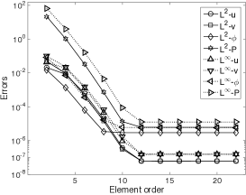
(a) Errors vs Element order

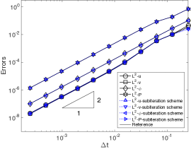
(b) Errors vs ${\Delta}t$

Figure 1: Spatial/temporal convergence tests: (a) $L^{2}$ and $L^{\infty}$ errors of flow variables versus element order (fixed $\Delta t=0.001$ and $t_{f}=0.1$); (b) $L^{2}$ errors of flow variables versus $\Delta t$ (fixed element order $22$ and $t_{f}=1$) and comparison with the sub-iteration method discussed in Remark 1.

In the spatial convergence test, we fix the integration time at $t_{f}=0.1$ and the time step size at $\Delta t=0.001$ ($100$ time steps), and vary the element order systematically between $2$ and $22.$ The same element order has been used for these two spectral elements. Figure 1(a) depicts the numerical errors at $t=t_{f}$ in $L^{2}$ and $L^{\infty}$ norms for different flow variables as a function of the element order. It is evident that within a specific range of the element order (below around $12$), the errors decrease exponentially with increasing element order, displaying an exponential convergence rate in space. Beyond the element order of about $12,$ the error curves level off as the element order further increases, showing a saturation caused by the temporal truncation error.

In the temporal convergence test, we fix the integration time at $t_{f}=1$ and the element order at a large value $22,$ and vary the time step size systematically between $\Delta t=2.44141\times 10^{-4}$ and $\Delta t=0.25.$ Figure 1(b) shows the numerical errors at $t=t_{f}$ in $L^{2}$ norm for different variables as a function of $\Delta t$ in logarithmic scales. It can be observed that the numerical errors exhibit a second order convergence rate in time.

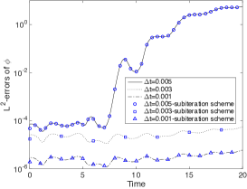
(a) Comparison of methods with and without sub-iterations

(b) Number of sub-iterations within a time step

Figure 2: Computations with sub-iterations: (a) Comparison of $L^{2}$ errors of $\phi$ between the method using approximation (72) and the sub-iteration method with several ${\Delta}t$ values; (b) Evolution of the number of sub-iterations needed within a time step over time for the sub-iteration method. Results are obtained with a fixed element order $22$ and $t_{f}=20.$ Those curves in (a) with legends not marked by “subiteration scheme” are obtained with the method using the approximation  (72).

As discussed in Section 2, two methods have been implemented for solving equation (70), based on a sub-iteration procedure as discussed in Remark 1 and based on the approximation (72) on $\partial\Omega$. The simulation results presented so far are obtained based on the method with the approximation (72) by default. To compare these two methods, in Figure 1(b) we have also included the numerical errors obtained with the sub-iteration method (marked by “subiteration scheme” in the legend). It is observed that the difference in the numerical errors between these two methods is negligible. In Figure 2(a) we compare the time histories of the $L^{2}$-errors for $\phi$ computed with several ${\Delta}t$ values for longer-time simulations ($t_{f}=20$) with both methods. We observe that the error histories of both methods essentially overlap with each other. In Figure 2(b), we plot the time histories of the number of sub-iterations needed for convergence within a time step for the sub-iteration method. The results indicate that for the smaller $\Delta t$ values around $2\sim 4$ sub-iterations are needed for convergence within a time step, while for the larger $\Delta t=0.005$ it can take $8$ or more sub-iterations within a time step. These results show that the method with the approximation (72) is clearly advantageous. It is cheaper computationally, and produces essentially the same simulation results.

The above numerical results indicate that the numerical algorithm developed herein exhibits a spatial exponential convergence rate and a temporal second-order convergence rate.

3.2 Capillary Wave Problem

Parameter	Value	Parameter	Value
$H_{0}$	0.01	$k_{w}$ (wave number)	$2\pi$
$\sigma$	1.0	$|\bm{g}_{r}|$ (gravity)	1.0
$\rho_{1}$	1.0	$\rho_{2}$	(varied)
$\mu_{1}$	0.01	$\mu_{2}$	$\mu_{1}\frac{\rho_{2}}{\rho_{1}}$
$\rho_{0}$	${\rm min}(\rho_{1},\rho_{2})$	$\nu_{m}$	$2\times\frac{{\rm max}(\mu_{1},\mu_{2})}{{\rm min}(\rho_{1},\rho_{2})}$
$C_{0}$	(varied)	$S$	$\sqrt{\frac{4\gamma_{0}\lambda}{m\Delta t}}$
$J$ (temporal order)	2	Number of elements	240
$m$	$5\times 10^{-4}$ or $10^{-5}$	$\eta$	(varied)
$\lambda$	$\frac{3}{2\sqrt{2}}\sigma\eta$	$\Delta t$	(varied)

Table 3: Simulation parameter values for the capillary wave problem.

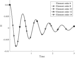
(a) $H$ vs element order

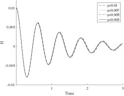
(b) $H$ vs interfacial thickness $\eta$

(c) $H$ vs simulation parameter $C_{0}$

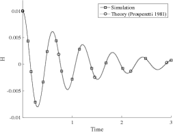
(d) $H$ vs Prosperetti’s exact solution

Figure 3: Capillary wave problem (matched density $\rho_{1}=\rho_{2}=1$): Comparison of capillary amplitude histories with different element orders (a), with different interfacial thickness $\eta$ values (b), with different $C_{0}$ (c) and between simulation result and Prosperetti’s exact solution. In (a), $\eta=0.005$, $C_{0}=0$; In (b), element order 10, $C_{0}=0$; In (c), $\eta=0.005,$ element order=10; In (d), element order 10, $\eta=0.005$, $C_{0}=0$.

In this subsection, we use the capillary wave problem, for which an exact solution is available, as a benchmark to test the accuracy of the proposed algorithm.

The problem setting is as follows. We consider two immiscible incompressible fluids contained in an infinite domain. The upper half of the domain is occupied by the lighter fluid (with density $\rho_{1}$), and the lower half of the domain is occupied by the heavier fluid (with density $\rho_{2}$). The gravity is assumed to be in the downward direction. The interface formed between these two fluids is perturbed from its horizontal equilibrium position by a small-amplitude sinusoidal wave form, and starts to oscillate at $t=0.$ The objective here is to study the motion of the interface over time.

In Prosperetti1981 an exact time-dependent standing-wave solution to this capillary wave problem was derived, under the condition that the two fluids must have matched kinematic viscosities (but their densities and dynamic viscosities can differ). To compare with Prosperetti’s exact physical solution (see Prosperetti1981 ), we adopt the following settings to simulate the capillary wave problem: (i) the capillary amplitude is small compared with the vertical dimension of the domain; and (ii) the kinematic viscosity $\nu$ satisfies $\nu=\frac{\mu_{1}}{\rho_{1}}=\frac{\mu_{2}}{\rho_{2}}$.

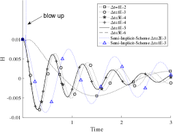
(a) $H$ vs various ${\Delta}t$

(b) Time history of $\xi^{n+1}$

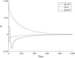
(c) $H$ vs large ${\Delta}t$

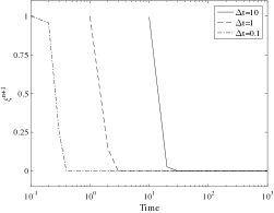
(d) Time history of $\xi^{n+1}$

Figure 4: Capillary wave problem (matched density $\rho_{1}=\rho_{2}=1$): (a) Comparison of capillary amplitude histories obtained with a range of smaller ${\Delta}t$, and also comparison with results obtained by the semi-implicit method from DongS2012 , and (b) corresponding time histories of $\xi^{n+1}$. (c) Comparison of capillary amplitude histories obtained with a range of large time step sizes ${\Delta}t$, and (d) corresponding time histories of $\xi^{n+1}$ in (d).

To simulate this problem, we consider a rectangular computational domain $\Omega=\{(x,y)|\;0\leq x\leq 1,-1\leq y\leq 1\}.$ The upper and bottom sides of the domain are assumed to be solid walls of neutral wettability. On the left and right sides, all the variables are assumed to be periodic at $x=0$ and $x=1.$ The equilibrium position of the fluid interface is assumed to coincide with $y=0.$ The initial perturbed profile of the fluid interface is given by $y=H_{0}\cos(k_{w}x)$, where $H_{0}=0.01$ is the initial amplitude, $\lambda_{w}=1$ is the wavelength of the perturbation profiles, and $k_{w}=2\pi/\lambda_{w}$ is the wave number. Note that the initial capillary amplitude $H_{0}$ is small compared with the dimension of the domain in the vertical direction. Therefore, the effect of the walls at the domain top/bottom will be small.

The computational domain is partitioned with $240$ quadrilateral elements, with $10$ and $12$ elements respectively in $x$ and $y$ directions. The elements are uniform in the $x$ direction, and are non-uniform and clustered around the regions $-0.015\leq y\leq 0.015$ in the $y$ direction. In the simulations, the external body force $\bm{f}$ in equation (7) is set to $\bm{f}=\rho\bm{g}_{r},$ where $\bm{g}_{r}$ is the gravitational acceleration, and the source term in equation (1c) is set to $g=0.$ On the upper and bottom wall, the boundary condition (9) with $\bm{w}=\bm{0}$ is imposed for the velocity, and the boundary conditions (10) and (11) with $d_{a}=d_{b}=0$ are imposed for the phase field functions. The initial velocity is set to zero, and the initial phase field function is prescribed as follows:

$$\phi(\bm{x},0)=\tanh\frac{y-H_{0}\cos(k_{w}x)}{\sqrt{2}\eta}.$$ (99)

We list in Table 3 the values for the physical and numerical parameters involved in this problem.

Let us first focus on the case with a matched density for the two fluids, i.e., $\rho_{1}=\rho_{2}=1$, and study the effects of several parameters on the simulation results with the data from Figures 3 and 4. Figure 3(a) shows a spatial resolution test. Here we compare the time histories of the capillary wave amplitude obtained with several element orders ranging from 6 to 14 in the simulations. These results are obtained with a fixed mobility $m=5\times 10^{-4},$ interfacial thickness $\eta=0.005,$ ${\Delta}t=10^{-5}$ and $C_{0}=0.$ The history curves corresponding to different element orders overlap with one another (with elements orders $8$ and above), suggesting independence of the results with respect to the grid resolution. In the forthcoming simulations, we will fix element order equal to $10$.

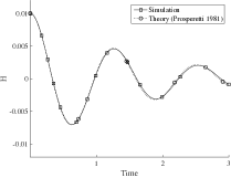
(a) $(\rho_{1},\rho_{2})=(1,10)$

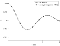
(b) $(\rho_{1},\rho_{2})=(1,100)$

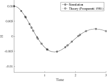
(c) $(\rho_{1},\rho_{2})=(1,1000)$

Figure 5: Capillary wave problem (different density ratios): Comparison of capillary amplitude histories with Prosperetti’s exact solution for density ratios (a) $\frac{\rho_{2}}{\rho_{1}}=10$ (b) $\frac{\rho_{2}}{\rho_{1}}=100$ (c) $\frac{\rho_{2}}{\rho_{1}}=1000$. The simulation results are obtained with $\Delta t=10^{-5}$ for (a)-(b) and $\Delta t=2.5e-6$ for (c).

Figure 3(b) shows the effect of the interfacial thickness scale $\eta$ on the simulation results. In this figure we compare time histories of the capillary amplitude obtained with the interfacial thickness scale parameter $\eta$ ranging from $0.01$ to $0.003.$ These results correspond to a fixed mobility $5\times 10^{-4},$ ${\Delta}t=10^{-5}$ and $C_{0}=0.$ Some influence on the amplitude and the phase of the history curves can be observed as $\eta$ decreases from $0.01$ to $0.007.$ From $\eta=0.007$ and below, on the other hand, the history curves essentially overlap with one another and little difference can be discerned among them, suggesting a convergence of the results with respect to $\eta.$

Figure 3(c) demonstrates the effect of the parameter $C_{0}$ on the simulation results with a fixed $m=5\times 10^{-4}$ and $\eta=0.005$. No difference can be discerned among the numerical results obtained with different $C_{0}$ values. In the following simulations, we will employ $C_{0}=0.$

In Figure 3(d), we compare the time history of the capillary amplitude obtained using $m=5\times 10^{-4}$ and $\eta=0.005$ with the exact solution by Prosperetti1981 . The difference between the numerical result and the theoretic solution is negligible, showing that our method produces physically accurate numerical results.

Next, we demonstrate the robustness of our method with various time step sizes, ranging from very small to very large values. In Figure 4(a), we show time histories of the capillary amplitude obtained with time step size in a range of smaller values, $\Delta t=10^{-2}\sim 5\times 10^{-6}$. The results correspond to a fixed mobility $m=5\times 10^{-4}$ and interfacial thickness $\eta=0.005$ in the simulations. For comparison, this figure also includes the results obtained using the semi-implicit method from DongS2012 with time step sizes $\Delta t=0.001$ and $0.002$. All the simulations using the current method are stable, and the time history curves collapse to a single one when the time step size is reduced to $\Delta t=10^{-4}$ and below, suggesting convergence with respect to $\Delta t$. In contrast, the simulation using the semi-implicit scheme of DongS2012 blows up with $\Delta t=0.002$. With $\Delta t=0.001$, the semi-implicit simulation is stable. But the resultant history curve contains considerably larger errors in both amplitude and phase, with respect to the theoretical solution, than the result obtained using the current method with the same time step size. In Figure 4(b), we plot the corresponding time histories of $\xi^{n+1}=\frac{R^{n+1}}{\sqrt{E^{n+1}}}$ computed from equation (85). Note that $\xi^{n+1}$ should physically take the unit value, because $R(t)=\sqrt{E(t)}$ by definition when deriving the dynamic equation about $R(t)$. A substantial deviation of $\xi^{n+1}$ from the unit value indicates that $R(t)$ is no longer an accurate approximation of $\sqrt{E(t)}$, and therefore the simulation will contain significant errors. So the value of $\xi^{n+1}$ is a good indicator of the accuracy of the simulation results. We observe that when ${\Delta}t$ is small (less than $10^{-3}$), $\xi^{n+1}$ is identical to $1.$ But when ${\Delta}t=10^{-2}$, $\xi^{n+1}$ decreases sharply to $0.2$ and then remains at that level over time. This suggests that the simulation is no longer accurate and the result contains significant errors with this $\Delta t$.

Thanks to its energy-stable nature, our algorithm can produce stable simulation results even with very large time step sizes. This is demonstrated by Figures 4(c) and (d) for a range of large time step sizes. Here we increase the time step sizes to $\Delta t=0.1,1,10$ and depict the time histories of the capillary amplitude in Figure 4 (c) for a much longer simulation (up to $t=1000$). The long time histories demonstrate that the computations with these large ${\Delta}t$ values are indeed stable using the current algorithm. On the other hand, because these time step sizes are very large, we do not expect that these results will be accurate. It is observed that the characteristics of these history curves are quite different from those obtained with smaller time step sizes (comparing with e.g. Figure 4(a)). Figure 4(d) shows the corresponding time histories of $\xi^{n+1}$ with this range of large $\Delta t$ values. The behaviors of $\xi^{n+1}$ are quite different from those obtained with small ${\Delta}t$ (see Figure 4(b)). The general characteristics seem to be that, when $\Delta t$ increases to a fairly large value the computed $\xi^{n+1}$ would decrease over time and its history curve would level off at a certain value for a given ${\Delta}t$. With a larger ${\Delta}t$, the $\xi^{n+1}$ history tends to level off at a smaller value. With very large ${\Delta}t$ values, $\xi^{n+1}$ will essentially tend to zero. Note that these simulations are performed using the method with the approximation (72) when solving equation (70). The results with the large $\Delta t$ values demonstrate that the approximation (72) on the boundary does not weaken the stability of our method.

Let us next investigate the effect of the density ratio on the dynamics of the fluid interface. In these tests we fix $\rho_{1}=1$ and $\mu_{1}=0.01$ for the first fluid and vary the density $\rho_{2}$ and the dynamic viscosity $\mu_{2}$ of the second fluid systematically while the relation $\nu=\frac{\mu_{1}}{\rho_{1}}=\frac{\mu_{2}}{\rho_{2}}$ is maintained as required by the theoretic solution in Prosperetti1981 . In Figure 5, we show the time histories of the capillary amplitudes corresponding to density ratios ${\rho_{2}}/{\rho_{1}}=10,100,1000$, and compare them with the theoretical solutions from Prosperetti1981 . The simulation results are obtained with a fixed interfacial thickness $\eta=0.005$, mobility $m=10^{-5}$, and $\Delta t=10^{-5}$ for Figures 5(a)-(b) and $\Delta t=2.5\times 10^{-6}$ for Figure 5(c). We observe that the density contrasts have a dramatic effect on the motions of the interfaces. Increase in the density ratio increases the oscillation period and the attenuation of the amplitude becomes more pronounced. It can also be observed that the history curves from the simulations agree well with those of the exact solutions for all the density ratios, indicating that our method has captured the dynamics of the fluid interfaces correctly.

The capillary wave problem and in particular the comparisons with Prosperetti’s exact solution for this problem demonstrate that our algorithm produces physically accurate results for a wide range of density ratios (up to density ratio $1000$ tested here), and that it is stable for large time step sizes in long-time simulations.

3.3 Rising Air Bubble in Water

Parameter	Value	Parameter	Value
$(x_{0},y_{0})$	$(0.08,-0.3)$	$R_{0}$	$0.1$
$\sigma$	10	$|\bm{g}_{r}|$ (gravity)	1.0
$\rho_{1}$	1.0	$\rho_{2}$	$100$ or $1000$
$\mu_{1}$	0.01	$\mu_{2}$	$0.5$
$\rho_{0}$	${\rm min}(\rho_{1},\rho_{2})$	$\nu_{m}$	$2\times\frac{{\rm max}(\mu_{1},\mu_{2})}{{\rm min}(\rho_{1},\rho_{2})}$
$C_{0}$	$0$	$S$	$\sqrt{\frac{4\gamma_{0}\lambda}{m\Delta t}}$
$m$	$10^{-7}$	$\eta$	$0.01$
$\lambda$	$\frac{3}{2\sqrt{2}}\sigma\eta$	$\Delta t$	$5\times 10^{-5}$ (or varied)
$J$ (temporal order)	2	Number of elements	146
Element order	$10$

Table 4: Simulation parameter values for the rising bubble problem.

In this section, we test the proposed method using a two-phase flow problem in an irregular domain, involving realistically large density ratios and viscosity ratios encountered in the physical world. The density ratio and viscosity ratio of the two fluids correspond to those of the air and water in the majority of cases considered here. But for some cases the density ratio of the fluids will also be artificially varied, and for those cases we will still refer to these fluids as air and water.

To be more specific, we consider a rectangular domain, defined by $\Omega=\big{\{}(x,y)|-0.25\leq x\leq 0.25,\;-0.5\leq y\leq 0.25\big{\}}$. The top and bottom of the domain are solid walls, and in the horizontal direction it is periodic. A square region inside this domain, centered at $(0,0)$ with a dimension $l=0.1$ on each side, is occupied by a solid object; see Figure 6(a) for a sketch of the configuration. The flow (and computational) domain consists of the space between the interior solid-square object and the top/bottom walls on the outside. This domain is filled with water, which traps an air bubble inside; see Figure 6(a). The gravity is assumed to point downward. At $t=0,$ the air bubble is circular and centered at $(x_{0},y_{0})=(0.08,-0.3)$ with a radius $R_{0}=0.1,$ and it is at rest. Then the system is released, and the air bubble rises through the water and interacts with the walls of the interior object and the outside domain wall. We would like to simulate this dynamic process using the current method.

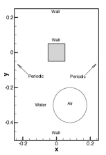
(a) $t=0.00005$

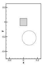
(b) $t=1.0$

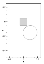
(c) $t=1.6$

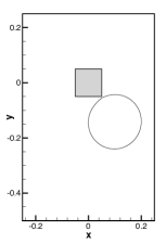
(d) $t=1.7$

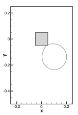
(e) $t=1.75$

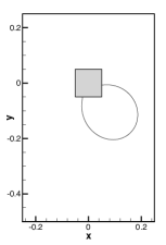
(f) $t=1.9$

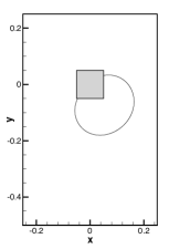
(g) $t=2.1$

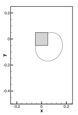
(h) $t=2.25$

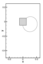
(i) $t=2.85$

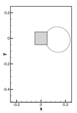
(j) $t=3.25$

(k) $t=4.2$

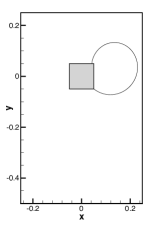
(l) $t=6.0$

Figure 6: Time sequence of snapshots of an air bubble rising in water with a smaller density contrast $(\rho_{1},\rho_{2})=(1,100)$. Fluid interface is visualized by the contour levels $\phi(\bm{x},t)=0$.

The computational domain is partitioned with $146$ quadrilateral elements, with $10$ and $15$ uniform elements respectively in the $x$ and $y$ directions (with $4$ elements excluded from the region of the solid square). In the simulations, the external body force $\bm{f}$ in equation (7) is set to $\bm{f}=\rho\bm{g}_{r},$ where $\bm{g}_{r}$ is the gravitational acceleration and $\rho$ is the mixture density. The source term in equation (1c) is set to $g=0.$ We further assume that all the wall surfaces have a neutral wettability. In other words, if the air-water interface intersects the outside domain walls or the walls of the interior solid square, the contact angle on the wall would be $90^{o}.$ On the outside top/bottom walls and the surfaces of the interior solid square, the boundary condition (9) with $\bm{w}=\bm{0}$ is imposed for the velocity, and the boundary conditions (10) and (11) with $d_{a}=d_{b}=0$ are imposed for the phase field function. On the two sides of the domain in the horizontal direction ($x=\pm 0.25$) periodic boundary conditions are imposed for all flow variables. The initial velocity is set to zero, and the initial phase field function is prescribed as follows:

$$\phi(\bm{x},0)=-\tanh\frac{\sqrt{(x-x_{0})^{2}+(y-y_{0})^{2}-R_{0}}}{\sqrt{2}\eta}.$$ (100)

In the simulations, we treat air as the first fluid and water as the second fluid. We employ a viscosity ratio $\frac{\mu_{2}}{\mu_{1}}=50$ and a density ratio $\frac{\rho_{2}}{\rho_{1}}=1000$ for the air and water. Another artificial density ratio $\frac{\rho_{2}}{\rho_{1}}=100$ is also considered in the tests. The normalized physical and numerical parameters involved in this problem are listed in Table 4.

We first consider the case with an artificially smaller density contrast for air and water, $(\rho_{1},\rho_{2})=(1,100).$ Figure 6 is a sequence of snapshots in time of the fluid interfaces for this case, visualized by the contour level $\phi(\bm{x},t)=0.$ These results are computed with a time step size $\Delta t=5\times 10^{-5}$. From $t=0$ to about $t=1.6$ (Figure 6(a)-(c)), the air bubble rises through the water inside the container, and gradually approaches the bottom right corner of the interior square object. A slight deformation of the bubble can be noticed. The air bubble collides onto the square object at approximately $t=1.7$ (Figure 6(d)), and is drawn rapidly towards the cylinder due to the strong effect of surface tension (Figure 6(e)-(g)). From $t=2.25$ to $t=6$ (Figure 6(h)-(l)), the air bubble slides on the bottom surface of the interior square object, and moves toward the right. It eventually settles down at an equilibrium position, still attached to the right and top sides of the solid square.

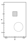
(a) $t=0.00005$

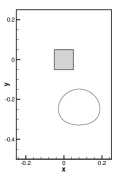
(b) $t=0.5$

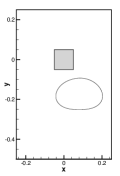
(c) $t=0.85$

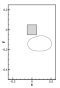
(d) $t=1.0$

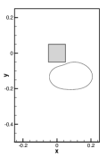
(e) $t=1.1$

(f) $t=1.2$

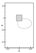
(g) $t=1.3$

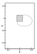
(h) $t=1.55$

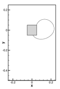
(i) $t=1.8$

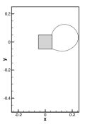
(j) $t=1.9$

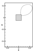
(k) $t=2.7$

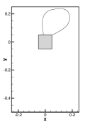
(l) $t=3.25$

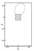
(m) $t=3.55$

(n) $t=3.6$

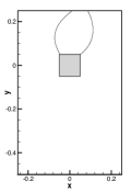
(o) $t=3.65$

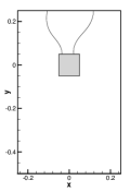
(p) $t=3.95$

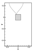
(q) $t=4.4$

(r) $t=4.45$

(s) $t=5.35$

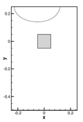
(t) $t=6.0$

Figure 7: Time sequence of snapshots of an air bubble rising in water with a normal density contrast $(\rho_{1},\rho_{2})=(1,1000)$. Shown are the contour levels $\phi(\bm{x},t)=0$.

Let us now look into the case with a normal density contrast for air and water, $(\rho_{1},\rho_{2})=(1,1000).$ In Figure 7, we plot a temporal sequence of snapshots of the air-water interface for this case, computed with $\Delta t=5\times 10^{-5}$. The dynamical characteristics observed here are notably different and much more complicated than those in the previous case with a smaller density contrast. As the air bubble rises through the water from $t=0$ to $t=0.85$ (Figure 7(a)-(c)), the bubble experiences more considerable deformation and one can observe a flat bottom side in the shape of the bubble. Notice also that the rise of the bubble is more rapid than in the previous case. From $t=1.0$ to $t=1.1$ (Figure 7(d)-(e)), the air bubble approaches the bottom right corner of the solid square, and an indentation appears on the shoulder of the bubble. The air bubble collides onto the square and is attached to its surface near the bottom right corner from $t=1.2$ to $t=1.55$ (Figure 7(f)-(h)). Afterwards, the bubble slides on the surface of the solid square, from the bottom to the right and then to the top of the interior square (Figure 7(g)-(m)). The bubble deformation is very pronounced during this process. Due to strong buoyancy, the bubble is stretched upward while still attached to the top surface of the solid square, and it approaches the top wall of the domain (Figure 7(m)). From $t=3.6$ to $t=4.4$ (Figure 7(m)-(q)), the air bubble touches the upper domain wall and forms contact lines on that wall. Simultaneously, the area of contact between the bubble and the top surface of the interior square shrinks, and the bubble deforms into a funnel (Figure 7(p)-(q)). From $t=4.45$ to $t=6.0$ (Figure 7(r)-(t)), the air bubble detaches from the interior solid square, and forms a dome attached to the upper domain wall over time.

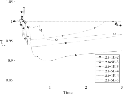
Figure 8: Comparison of time histories of $\xi^{n+1}$ obtained with various time step sizes ${\Delta}t=10^{-2}\sim 5\times 10^{-5}$ for the rising air bubble problem with density contrast $(\rho_{1},\rho_{2})=(1,1000)$.

In order to demonstrate the robustness of our method, we have performed tests using the second case $(\rho_{1},\rho_{2})=(1,1000)$ for various time step sizes ranging from ${\Delta}t=10^{-2}$ to $5\times 10^{-5}$. Figure 8 is a comparison of the time histories of $\xi^{n+1}$ for each time step size. We observe that even with large time step sizes (e.g. ${\Delta}t=10^{-2}),$ the computation is stable. We can observe that when ${\Delta}t$ is relatively small (${\Delta}t\leq 10^{-4}$), the computed $\xi^{n+1}$ is identical to $1$. For larger ${\Delta}t$, the computed values for $\xi^{n+1}$ initially oscillate near $1$ (from $t=0.2$ to $t=0.4$), and then decreases and settles to some levels less than $1$ over a long time. With a larger $\Delta t$ we generally attain a $\xi^{n+1}$ level over time that tends to be smaller.

Remark 2.

The computational cost for solving the nonlinear equation (85) using the Newton’s method, including the computations for the coefficients involved therein for preparation of the Newton solver, is small compared with the total cost within each time step. For example, with the same computational setting for producing the results of Figure (7) for the rising air bubble problem, the time spent in the Newton solver (including the time spent on computing the coefficients in equation (85)) per time step accounts for about $8\%$ of the total time per time step with our current method. The total wall time per time step is $0.3$ seconds on the average, in which around $0.024$ seconds is spent in the Newton solution for equation (85). Of the time spent in the Newton method, essentially all is spent on computing the coefficients involved in the nonlinear equation (85), and the actual Newton iteration time is negligible.

4 Concluding Remarks

In this paper we have developed an energy-stable scheme for approximating the coupled system of Navier-Stokes/Cahn-Hilliard equations for incompressible two-phase flows with different densities and viscosities for the two fluids. The scheme employs a scalar-valued auxiliary variable in the formulation, and it satisfies a discrete energy stability property regardless of the time step sizes. The scheme allows an efficient solution procedure and is computationally attractive. Within a time step, it computes two copies of the flow variables (velocity, pressure, phase field function), by solving individually a linear algebraic system involving a constant and time-independent coefficient matrix for each of these field functions. The coefficient matrices involved in these linear systems only need to be computed once and they can be pre-computed, even with large density ratios and large viscosity ratios. Additionally, the algorithm requires the solution of a nonlinear algebraic equation about a scalar-valued number using the Newton’s method within each time step. The computational cost for this nonlinear solver is very low, accounting for around $8\%$ of the total solver time per time step, because this nonlinear equation is about a scalar number, not a field function. Because of these properties, the presented method is robust and computationally efficient.

We have tested the proposed method with extensive numerical experiments for several two-phase flow problems involving large density ratios and viscosity ratios. In particular, by comparing with Prosperetti’s exact solution for the capillary wave problem, we have shown that our method produces physically accurate results for various density ratios and viscosity ratios. Large time step sizes have been tested with the proposed method in two-phase simulations. While the simulation results cannot be expected to be accurate at those time step sizes, the computations have been shown to be stable nonetheless, verifying the robustness of the method developed herein.

Some comments concerning the auxiliary variable strategy are in order. It should be noted that the coupled Navier-Stokes/Cahn-Hilliard equations are not a gradient-type system. As such, we find that the auxiliary variable formulation as described in e.g. ShenXY2018 for gradient flows does not carry over to Navier-Stokes equations or two-phase flows. Two lessons are learned:

• Attempts to reformulate the viscous terms in these equations using the auxiliary variable, which is analogous to the auxiliary-variable treatments of the dissipation terms in the evolution equation for gradient flows, lead to very poor simulation results. A viable strategy for the two-phase governing equations is to employ the auxiliary variable to reformulate the convection terms in the momentum equation and the phase field equation. The integral form of the dynamic equation for the scalar-valued auxiliary energy variable provides a great deal of flexibility to be commensurate with the corresponding treatments of various terms in the momentum and phase-field equations to ensure a discrete energy stability property.

• When solving for the scalar-valued number, $\xi^{n+1}=\frac{R^{n+1}}{\sqrt{E^{n+1}}}$, it should be noted that in the implementation we have employed equation (82), which is based on the transformed dynamic equation (50) instead of the original equation (32). While equations (32) and (50) are mathematically equivalent, we find that in practice the method is more robust if the implementation is based on the transformed equation (50).

An important implication of the current method lies in the following. It demonstrates that the energy-stable schemes for two-phase flows can also become computationally efficient, eliminating the expensive re-computations for the coefficient matrices involved in the associated linear algebraic systems. In terms of the amount of operations per time step, the energy-stable schemes can be competitive. For example, within each time step, the amount of operations involved in the current method is approximately twice that of the semi-implicit method of DongS2012 , which is only conditionally stable, or slightly larger than that due to the extra nonlinear equation about a scalar-valued number.

References

- [1] H. Abels, H. Garcke, and G. Grün. Thermodynamically consistent, frame indifferent diffuse interface models for incompressible two-phase flows with different densities. Mathematical Models and Methods in Applied Sciences, 22:1150013, 2012.
- [2] G.L. Aki, W. Dreyer, and J. Giesselmann. A quasi-incompressible diffuse interface model with phase transition. Mathematical Models and Methods in Applied Sciences, 24:827–861, 2014.
- [3] S. Aland and F. Chen. An efficient and energy stable scheme for a phase-field model for the moving contact line problem. International Journal for Numerical Methods in Fluids, 81:657–671, 2016.
- [4] S.M. Allen and J.W. Cahn. A miscopic theory for antiphase boundary motion and its application to antiphase domain coarsening. Acta Metallurgica, 27:1085–1095, 1979.
- [5] D.M. Anderson, G.B. McFadden, and A.A. Wheeler. Diffuse-interface methods in fluid mechanics. Annual Review of Fluid Mechanics, 30:139–165, 1998.
- [6] V.E. Badalassi, H.D. Ceniceros, and S. Banerjee. Computation of multiphase systems with phase field models. Journal of Computal Physics, 190:371–397, 2003.
- [7] F. Boyer and S. Minjeaud. Numerical schemes for a three component cahn-hilliard model. ESAIM: M2AN, 45:697–738, 2011.
- [8] J.W. Cahn and J.E. Hilliard. Free energy of a nonuniform system. I interfacial free energy. Journal of Chemical Physics, 28:258–267, 1958.
- [9] H. Ding, P.D.M. Spelt, and C. Shu. Diffuse interface model for incompressible two-phase flows with large density ratios. Journal of Computal Physics, 226:2078–2095, 2007.
- [10] S. Dong. On imposing dynamic contact-angle boundary conditions for wall-bounded liquid-gas flows. Computer Methods in Applied Mechanics and Engineering, 247–248:179–200, 2012.
- [11] S. Dong. An efficient algorithm for incompressible N-phase flows. Journal of Computational Physics, 276:691–728, 2014.
- [12] S. Dong. An outflow boundary condition and algorithm for incompressible two-phase flows with phase field approach. Journal of Computational Physics, 266:47–73, 2014.
- [13] S. Dong. Physical formulation and numerical algorithm for simulating N immiscible incompressible fluids involving general order parameters. Journal of Computational Physics, 283:98–128, 2015.
- [14] S. Dong. Multiphase flows of N immiscible incompressible fluids: a reduction-consistent and thermodynamically-consistent formulation and associated algorithm. Journal of Computational Physics, 361:1–49, 2018.
- [15] S. Dong and J. Shen. A time-stepping scheme involving constant coefficient matrices for phase field simulations of two-phase incompressible flows with large density ratios. Journal of Computational Physics, 231:5788–5804, 2012.
- [16] Y. Gong, J. Zhao, and Q. Wang. An energy stable algorithm for a quasi-incompressible hydrodynamic phase-field model of viscous fluid mixtures with variable densities and viscosities. Computer Physics Communications, 219:20–34, 2017.
- [17] Y. Gong, J. Zhao, X. Yang, and Q. Wang. Fully discrete second-order linear schemes for hydrodynamic phase field models of binary viscous fluid flows with variable densities. SIAM J. Sci. Comput., 40:B138–B167, 2018.
- [18] G. Grun and F. Klingbeil. Two-phase flow with mass density contrast: stable schemes for a thermodynamically consistent and frame-indifferent diffuse-interface model. J. Comput. Phys., 257:708–725, 2014.
- [19] J.L. Guermond and L. Quartapelle. A projection FEM for variable density incompressble flows. Journal of Computal Physics, 165:167–188, 2000.
- [20] Z. Guo, P. Lin, J. Lowengrub, and S.M. Wise. Mass conservative and energy stable finite difference methods for the quasi-incompressible navier-stokes-cahn-hilliard system: primitive and projecton-type schemes. Comput. Meth. Appl. Mech. Engrg., 326:144–174, 2017.
- [21] Z. Guo, P. Lin, and J.S. Lowengrub. A numerical method for the quadi-incompressible cahn-hilliard-navier-stokes equations for variable density flows with a discrete energy law. J. Comput. Phys., 276:486–507, 2014.
- [22] D. Han, A. Beylev, X. Yang, and Z. Tan. Numerical analysis of second order, fully discrete energy stable schemes for phase field models of two-phase incompressible flows. Journal of Scientific Computing, 70:965–989, 2017.
- [23] D. Jacqmin. Calculation of two-phase navier-stokes flows using phase-field modeling. Journal of Computal Physics, 155:96–127, 1999.
- [24] G.E. Karniadakis and S.J. Sherwin. Spectral/hp element methods for computational fluid dynamics, 2nd edition. Oxford University Press, 2005.
- [25] J. Kim and J. Lowengrub. Phase field modeling and simulation of three-phase flows. Interfaces and Free Boundaries, 7:435–466, 2005.
- [26] L. Lin, Z. Yang, and S. Dong. Numerical approximation of incompressible Navier-Stokes equations based on an auxiliary energy variable. arXiv:1804.10859.
- [27] C. Liu and J. Shen. A phase field model for the mixture of two incompressible fluids and its approximation by a fourier-spectral method. Physica D, 179:211–228, 2003.
- [28] C. Liu, J. Shen, and X. Yang. Decoupled energy stable schemes for a phase-field model of two-phase incompressible flows with variable density. Journal of Scientific Computing, 62:601–622, 2015.
- [29] J. Lowengrub and L. Truskinovsky. Quasi-incompressible Cahn-Hilliard fluids and topological transitions. Proceedings of Royal Society London A, 454:2617–2654, 1998.
- [30] S.J. Osher and J.A. Sethian. Fronts propagating with curvature dependent speed: algorithms based on hamilton-jacobi formulations. Journal of Computal Physics, 79:12–49, 1988.
- [31] A. Prosperetti. Motion of two superposed viscous fluids. Physics of Fluids, 24:1217–1223, 1981.
- [32] T. Qian, X.-P. Wang, and P. Sheng. A variational approach to moving contact line hydrodynamics. Journal of Fluid Mechanics, 564:333–360, 2006.
- [33] L. Rayleigh. On the theory of surface forces II. Phil. Mag., 33:209, 1892.
- [34] M. Schorpour Roudbari, G. Simsek, E.H. van Brummelen, and K.G. van der Zee. Diffuse-interface two-phase flow models with different densities: a new quasi-incompressible form and a linear energy-stable method. Mathematocal Models and Methods in Applied Sciences, 28:733–770, 2018.
- [35] A.J. Salgado. A diffuse interface fractional time-stepping technique for incompressible two-phase flows with moving contact lines. ESAIM: Mathematical Modeling and Numerical Analysis, 47:743–769, 2013.
- [36] R. Scardovelli and S. Zaleski. Direct numerical simulation of free-surface and interfacial flow. Annu. Rev. Fluid Mech., 31:567–603, 1999.
- [37] J.A. Sethian and P. Semereka. Level set methods for fluid interfaces. Annu. Rev. Fluid Mech., 35:341–372, 2003.
- [38] J. Shen, J. Xu, and J. Yang. The scalar auxiliary variable (sav) approach for gradient flows. Journal of Computational Physics, 353:407–416, 2018.
- [39] J. Shen and X. Yang. Energy stable schemes for cahn-hilliard phase-field model of two-phase incompressible flows. Chin. Ann. Math. Ser. B, 31:743–758, 2010.
- [40] J. Shen and X. Yang. A phase-field model and its numerical approximation for two-phase incompressible flows with different densities and viscosities. SIAM J. Sci. Comput., 32:1159–1179, 2010.
- [41] J. Shen and X. Yang. Decoupled, energy stable schemes for phase-field models of two-phase incompressible flows. SIAM J. Numer. Anal., 53:279–296, 2015.
- [42] J. Shen, X. Yang, and Q. Wang. On mass conservation in phase field models for binary fluids. Comminications in Computational Physics, 13:1045–1065, 2013.
- [43] G. Tryggvason, B. Bunner, and A. Esmaeeli et al. A front-tracking method for computations of multiphase flow. Journal of Computal Physics, 169:708–759, 2001.
- [44] J. van der Waals. The thermodynamic theory of capillarity under the hypothesis of a continuous density variation. J. Stat. Phys., 20:197–244, 1893.
- [45] X. Yang. Linear, first and second-order, unconditionally energy stable numerical schemes for the phase field model of homopolymer blends. Journal of Computational Physics, 327:294–316, 2016.
- [46] X. Yang and H. Yu. Efficient second order unconditionally stable schemes for a phase field moving contact line model using an invariant energy quadratization approach. SIAM J. Sci. Comput., 40:B889–B914, 2018.
- [47] H. Yu and X. Yang. Numerical approximations for a phase-field moving contact line model with variable densities and viscosities. J. Comput. Phys., 334:665–686, 2017.
- [48] P. Yue, J.J. Feng, C. Liu, and J. Shen. A diffuse-interface method for simulating two-phase flows of complex fluids. Journal of Fluid Mechanics, 515:293–317, 2004.