Kink-kink and kink-antikink interactions with long-range tails

Abstract

In this Letter, we address the long-range interaction between kinks and antikinks, as well as kinks and kinks, in $\varphi^{2n+4}$ field theories for $n>1$. The kink-antikink interaction is generically attractive, while the kink-kink interaction is generically repulsive. We find that the force of interaction decays with the $(\frac{2n}{n-1})$th power of their separation, and we identify the general prefactor for arbitrary $n$. Importantly, we test the resulting mathematical prediction with detailed numerical simulations of the dynamic field equation, and obtain good agreement between theory and numerics for the cases of $n=2$ ($\varphi^{8}$ model), $n=3$ ($\varphi^{10}$ model) and $n=4$ ($\varphi^{12}$ model).

Introduction.

The study of field-theoretic models with polynomial potentials has been a topic of wide appeal across a diverse span of theoretical physics areas, including notably cosmology, condensed matter physics and nonlinear dynamics vilenkin01 ; manton_book ; eilbeck . Arguably, the most intensely studied model in this class is the quartic (double well) potential, the so-called $\varphi^{4}$ model, connected to the phenomenological Ginzburg–Landau theory GinzburgLandau ; Tinkham , among numerous other applications Bishop80 ; K75 ; csw ; vach08 . While the $\varphi^{4}$ model has a time-honored history in its own right ourbook , more recently, higher-order field theories have emerged as models of phase transitions khare relevant to material science gl ; ferro ; iso (see also (ourbook, , Chap. 11) and Katsnelson14 ), or in quantum mechanical problems (including supersymmetric ones) bazeia17 , among others. There, the prototypical example has been the $\varphi^{6}$ field-theoretic model, which has led to numerous insights and novel possibilities with respect to the spectral properties DDKCS and wave interactions phi6 .

Scattering of solitary waves (topological defects or otherwise) is a long-standing topic of active research amin , starting from the early works K75 ; csw . Our aim here is to go beyond the “classical” models, in a direction that, admittedly, has already seen some significant activity lohe ; mello ; bazeia06-11 ; Gomes.PRD.2012 ; khare ; GaLeLi ; bazeia18 ; Belendryasova.2019 . One of the particularly appealing aspects of this research program (aside from its potential above-mentioned applications in material science or high-energy physics/quantum mechanics) is that higher-order field theories possess topological defect solutions (kinks) with power-law tails, rather than the “standard” exponential tails that we are used to in the $\varphi^{4}$ and the (usual variants of) $\varphi^{6}$ field theories. The resulting dynamics set by the power-law tails endows topological defects with long-range interactions. Recently, a methodology for quantifying such kink-kink and kink-antikink interactions in the $\varphi^{8}$ model was proposed in manton . In our previous work ivan_longrange , we showed that there are some deep challenges in even initializing such topological defect configurations numerically. Thus, the initial conditions in a direct numerical simulation of interactions may substantially affect the nature of the observed interactions (cf. also earlier works including, e.g., Belendryasova.2019 ).

One of the related motivations of our study stems from the expectation that power-law tails may affect the physical properties of a system governed by higher-order field theories. For instance, the dynamics and interaction of domain walls in ferroelastic materials undergoing successive phase transitions ferro should affect the elastic properties in unusual ways. Similarly, the response of crystals undergoing isostructural transitions iso or the behavior of crystallization of chiral proteins proteins should be altered by the associated long-range interactions between domain walls.

The present effort provides an answer to the question of how kink-kink (K-K) and kink-antikink (K-AK) long-range (power-law) interactions occur in higher-order field theories that exhibit such topological defects. We consider particular (yet highly relevant to this problem) potentials where the highest power of $\varphi$ in the potential is $2n+4$ and we analyze the interaction for arbitrary $n\geq 2$. We find that kinks repel each other, while kinks and antikinks generically attract, in both cases with a power law decaying as the $(\frac{2n}{n-1})$th power of their mutual separation. Furthermore, we adapt the recent methodology of manton to the case of arbitrary $n\geq 2$, and we identify the prefactor (distinct for K-K and K-AK) of the corresponding power-law interaction force. Equally important, we resolve the “uncertainty” of the prefactor indicated in manton . We identify the most accurate asymptotic prefactor and test it against direct numerical simulations to find good agreement for $\varphi^{8}$ ($n=2$), $\varphi^{10}$ ($n=3$) and $\varphi^{12}$ ($n=4$) models, for both K-K and K-AK interactions. The increasing trend of the deviations between the two, as $n$ increases, is also explained.

First, we present our theoretical results. Then, we compare them to direct numerical simulations. Finally, we offer some conclusions and directions for future work.

Theoretical Analysis.

Consider a real scalar field $\varphi(x,t)$ in $(1+1)$ dimensional spacetime, its dynamics set by the Lagrangian density

$$\mathscr{L}=\frac{1}{2}\left(\frac{\partial\varphi}{\partial t}\right)^{2}-\frac{1}{2}\left(\frac{\partial\varphi}{\partial x}\right)^{2}-V(\varphi).$$ (1)

The dynamic equation of motion of this field is

$$\frac{\partial^{2}\varphi}{\partial t^{2}}=\frac{\partial^{2}\varphi}{\partial x^{2}}-\frac{\mathrm{d}V}{\mathrm{d}\varphi}.$$ (2)

The potential $V$ is, specifically, of the form

$$V(\varphi)=\frac{1}{2}(1-\varphi^{2})^{2}\varphi^{2n}.$$ (3)

This potential has three minima: $\bar{\varphi}_{1}=-1$, $\bar{\varphi}_{2}=0$, and $\bar{\varphi}_{3}=1$. Hence, there are two kinks in this model, $\varphi_{(-1,0)}(x)$ and $\varphi_{(0,1)}(x)$, and two corresponding antikinks, $\varphi_{(0,-1)}(x)$ and $\varphi_{(1,0)}(x)$. All of these defects exhibit one power-law and one exponential asymptotic decay to the respective equilibria ($0$ and $\pm 1$) as $|x|\to\infty$. We study the interaction force between the kink $\varphi_{(0,1)}(x)$ and the kink $\varphi_{(-1,0)}(x)$. Their time-dependent positions are $x=\pm A(t)$, respectively, and their long-range tails overlap. Similarly, for the K-AK interaction, we employ the antikink $\varphi_{(0,-1)}(x)$ and the corresponding mirror kink $\varphi_{(-1,0)}(x)$ located at $x=\pm A(t)$, respectively.

In ivan_longrange , the interaction via power-law tail asymptotics was studied numerically for $n=2$ ($\varphi^{8}$ model). In manton , the force between a well-separated kink-kink and kink-antikink was analyzed, again for $n=2$. Our aim here is to generalize the (most sophisticated among the different) approach(es) of the very recent work manton , and to calculate the result for arbitrary $n$. Then, we blend this theoretical analysis with the delicate computational approach from ivan_longrange to fully flesh out the K-K and K-AK long-range interactions in such higher-order field theoretic models involving power-law tails.

Below, we model the accelerating kink solution of Eq. (2) by a field of the form $\varphi(x,t)=\phi(y)$, where $y=x-A(t)$ and $\phi=\varphi_{(0,1)}$ or $\varphi_{(0,-1)}$.

Kink-Kink Interaction.

Substituting the kink profile into Eq. (2) yields the static equation for $\phi$:

$$\phi^{\prime\prime}+a\phi^{\prime}-\left.\frac{\mathrm{d}V}{\mathrm{d}\varphi}\right|_{\varphi=\phi}=0,$$ (4)

where $a=\ddot{A}$ is the acceleration (assumed small) and Lorentz contraction terms ($\propto\dot{A}^{2}$) have been neglected. Here, $\dot{A}=\mathrm{d}{A}/\mathrm{d}t$, and $\phi^{\prime}=\mathrm{d}\phi/\mathrm{d}y$. Following manton , the Bogomolny equation $\phi^{\prime}=(\mathrm{d}W/\mathrm{d}\varphi)|_{\varphi=\phi}$, where $V={(1/2)}(\mathrm{d}W/\mathrm{d}\varphi)^{2}$, is used to eliminate $\phi^{\prime}$ from Eq. (4). Treating $a$ as slowly varying, we define an effective potential $\tilde{V}(\phi)\approx V(\phi)-aW(\phi)$. Then, from the first integral of Eq. (4) (setting the constant of integration in the limit of $y\to\infty$), we obtain

$$\left(\frac{\mathrm{d}\phi}{\mathrm{d}y}\right)^{2}=2\tilde{V}(\phi)+2aW(1)\sim\phi^{2n}+\frac{4a}{(n+1)(n+3)}.$$ (5)

This calculation is asymptotic (dropping $\mathrm{o}(\phi^{2n})$ terms), using the fact that our chosen family of potentials is such that $V(\phi)\sim\frac{1}{2}\phi^{2n}$ as $\phi\to 0$. Meanwhile, the second term in Eq. (5) (from the contribution of $W(1)-W(0)$, independently of the normalization of $W$) is effectively proportional to the kink’s rest mass $M=2/[(n+1)(n+3)]$ (for arbitrary $n$). Requesting (as in manton ) that $\phi(y)$ should have the properties that $\phi(-A)=0$ while $\phi(0)$ diverges, we can re-arrange Eq. (5) into a quadrature:

$$\int_{0}^{\infty}\frac{\mathrm{d}\phi}{\sqrt{\phi^{2n}+\frac{4a}{(n+1)(n+3)}}}=A.$$ (6)

The change of variables $\phi=\left({4a}/[(n+1)(n+3)]\right)^{\frac{1}{2n}}\lambda$ in Eq. (6) yields

$$\left[\frac{4a}{(n+1)(n+3)}\right]^{\frac{1-n}{2n}}\int_{0}^{\infty}\frac{\mathrm{d}\lambda}{\sqrt{\lambda^{2n}+1}}=A.$$ (7)

The relevant integral can be computed as

$$\int_{0}^{\infty}\frac{\mathrm{d}\lambda}{\sqrt{\lambda^{2n}+1}}=\frac{\Gamma(\frac{n-1}{2n})\Gamma(\frac{1}{2n})}{2n\sqrt{\pi}},$$ (8)

yielding the acceleration during the K-K interaction:

$$a=\left[\frac{\Gamma(\frac{n-1}{2n})\Gamma(\frac{1}{2n})}{2n\sqrt{\pi}}\right]^{\frac{2n}{n-1}}\frac{(n+1)(n+3)}{4}A^{\frac{2n}{1-n}}.$$ (9)

For the $\varphi^{8}$ model, $n=2$, and Eq. (9) yields $a={44.3139}/{A^{4}}$. From Newton’s second law ($F=Ma$), the force is $F=\frac{2}{15}a={5.9085}/{A^{4}}$. Similarly, for the $\varphi^{10}$ model, $n=3$, and we get $a={16.5411}/{A^{3}}$ and $F=\frac{1}{12}a={1.3784}/{A^{3}}$. Finally, for the $\varphi^{12}$ model, $n=4$, and we get $a={16.1871}/{A^{8/3}}$ and $F=\frac{2}{35}a={0.9250}/{A^{8/3}}$.

Kink-Antikink Interaction.

The calculation in the K-AK case proceeds in the same way with the main difference that now $a=-\ddot{A}$ due to the attraction, in this case, between kink and antikink. From the corresponding version of Eq. (6), we have

$$\int_{\left[\frac{4a}{(n+1)(n+3)}\right]^{1/2n}}^{\infty}\frac{\mathrm{d}\phi}{\sqrt{\phi^{2n}-\frac{4a}{(n+1)(n+3)}}}=A.$$ (10)

Notice that, now, the integral must be from the turning point rather than from $0$, related to the sign change of the Bogomolny equation satisfied by the anti-kink.

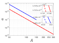
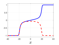
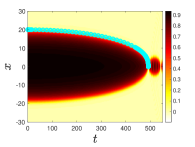
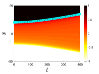
Figure 1: Top left is the log-log plot of the left kink acceleration $a$ as a function of $A$ for the kink-kink interaction (blue) and kink-antikink interaction (red) in the $\varphi^{8}$ model. The dashed lines are computed numerically, and the solid lines are computed analytically. Top right is the plot of the initializers for the kink-kink (K-K) (blue-solid) and kink-antikink (K-AK) (red-dashed) interaction. Bottom left is the space-time contour plot of the K-AK interaction, and the cyan curve with circle symbols is the plot of the solution to the initial value problem (IVP): $\ddot{x}(t)=-11.0785/x^{4}$, $x(0)=20$, $\dot{x}(0)=0$. Bottom right is space-time contour plot of the K-K interaction, and the cyan curve with circle symbols is the solution to the IVP: $\ddot{x}(t)=44.3139/x^{4}$, $x(0)=20$, $\dot{x}(0)=0$.

Using the same change of variables as above, Eq. (10) becomes

$$\left[\frac{4a}{(n+1)(n+3)}\right]^{\frac{1-n}{2n}}\int_{1}^{\infty}\frac{\mathrm{d}\lambda}{\sqrt{\lambda^{2n}-1}}=A.$$ (11)

Once again, the integral can be calculated:

$$\int_{1}^{\infty}\frac{\mathrm{d}\lambda}{\sqrt{\lambda^{2n}-1}}=\frac{-\sqrt{\pi}\,\Gamma(\frac{n-1}{2n})}{\Gamma(-\frac{1}{2n})},$$ (12)

yielding the acceleration during the K-AK interaction:

$$a=\left[\frac{-\sqrt{\pi}\,\Gamma(\frac{n-1}{2n})}{\Gamma(-\frac{1}{2n})}\right]^{\frac{2n}{{n-1}}}\frac{(n+1)(n+3)}{4}A^{\frac{2n}{1-n}}.$$ (13)

An intriguing observation stems from the ratio of Eqs. (13) and (9). In particular, using the well-known identities $a\Gamma(a)=\Gamma(a+1)$, and $\Gamma(a)\Gamma(1-a)=\pi/\sin(\pi a)$, we can express the ratio of the K-AK to K-K forces as

$$R=\frac{F_{\text{K-AK}}}{F_{\text{K-K}}}=-\left[\sin\left(\frac{\pi}{2n}\right)\right]^{\frac{2n}{n-1}}.$$ (14)

This expression suggests that, contrary to what is known about “standard” models such as sine-Gordon or $\varphi^{4}$ and their exponentially decaying kinks and antikinks manton_book ; eilbeck ; ourbook , here the ratio of the K-AK to K-K force is not equal to $1$, but rather decreases with $n$. Therefore, a fundamental characteristic of long-range-interacting kinks is that this feature becomes more dramatic (with the ratio, in principle, tending to $0$ as $n\rightarrow\infty$), the “heavier” the tails.

For $n=2$ ($\varphi^{8}$ model), from Eq. (13), we get $a={11.0785}/{A^{4}}$ and $F=-\frac{2}{15}a=-{1.4771}/{A^{4}}$. Similarly, for $n=3$ ($\varphi^{10}$ model), we get $a={2.0676}/{A^{3}}$ and $F=-\frac{1}{12}a=-{0.1723}/{A^{3}}$. Finally, for $n=4$ ($\varphi^{12}$ model), we get $a={1.2495}/{A^{8/3}}$ and $F=-\frac{2}{35}a=-{0.0714}/{A^{8/3}}$. Armed with these specific predictions for K-K and K-AK interactions, we turn to verification of our general theory via direct numerical simulations.

Numerical Results.

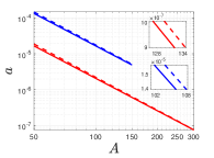
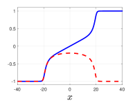
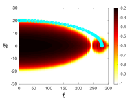
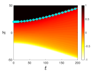
Figure 2: Equivalent of Fig. 1 for the $\varphi^{10}$ model. Bottom left is space-time contour plot of the K-AK interaction, and the cyan curve with circle symbols is the solution to the IVP: $\ddot{x}(t)=-2.0676/x^{3}$, $x(0)=20$, $\dot{x}(0)=0$. Bottom right is space-time contour plot of the K-K interaction, and the cyan curve with circle symbols is the solution to the IVP: $\ddot{x}(t)=16.5411/x^{3}$, $x(0)=20$, $\dot{x}(0)=0$.

Here, we deploy our recent methodology ivan_longrange , which is critical to obtaining accurate simulations of the interactions between topological defects with power-law tails (long-range interactions). Briefly, a pseudospectral differentiation matrix with periodic boundary conditions trefethen replaces the spatial derivatives in Eq. (2) on the interval $x\in[-200,200]$ with $N=2000$ discrete points (hence, the grid spacing is $\Delta x=0.2$). The resulting system of ODEs (after discretizing in $x$) is integrated numerically using Matlab’s ode45 solver with built-in error control.

Following ivan_longrange , for the K-AK interactions we start with a “split-domain” ansatz $\varphi_{\mathrm{split}}(x)=[1-H(x)]\varphi_{(-1,0)}(x)+H(x)\varphi_{(0,-1)}(x)$, where $H(x)$ is the Heaviside unit step function. That is, $\varphi_{\mathrm{split}}(x)=\varphi_{(-1,0)}(x)$ on the interval $(-\infty,0]$, while $\varphi_{\mathrm{split}}(x)=\varphi_{(0,-1)}(x)$ on the interval $(0,\infty)$. Then, $\varphi_{\mathrm{split}}(x)$ is used as the initializer for the Matlab function lsqnonlin, which minimizes (using nonlinear least squares) the $l_{2}$ norm of the discretized version of the opposite of the right-hand side of Eq. (2), subject to the two additional constraints of keeping the positions of the kink and antikink fixed. The result is a smoothed and minimized version of $\varphi_{\mathrm{split}}(x)$, which is then used as the initial condition for solving the PDE (2) numerically.

The K-K case is similar, except that $\varphi_{\mathrm{split}}(x)=[1-H(x)]\varphi_{(-1,0)}(x)+H(x)\varphi_{(0,1)}(x)$. As a result, there is a discontinuity at $x=0$, which becomes large for $\varphi^{10}$ and even larger for $\varphi^{12}$. With $N=2000$, lsqnonlin fails to converge for some cases; however, for smaller $N$ it does converge. Thus, the output from smaller $N$ can be used as the initializer for lsqnonlin with $N=2000$, which then converges quickly. Except for this detail, the procedure is the same as for the K-AK case. As explained in ivan_longrange , this type of minimization procedure is crucial in order to avoid inaccurate interaction observations stemming from a more naive sum or product (of kinks) ansatz.

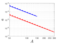
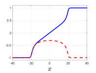
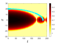
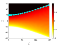
Figure 3: Equivalent of Figs. 1 and 2 for the $\varphi^{12}$ model. Bottom left is space-time plot of the K-AK interaction, and the cyan curve with circle symbols is the solution to the IVP: $\ddot{x}(t)=-1.2495/x^{8/3}$, $x(0)=20$, $\dot{x}(0)=0$. Bottom right is space-time contour plot of the K-K interaction, and the cyan curve with circle symbols is the solution to the IVP: $\ddot{x}(t)=16.1871/x^{8/3}$, $x(0)=20$, $\dot{x}(0)=0$.

In Figs. 1–3, the top-right panel shows the K-K and K-AK configuration initializers used to evolve the PDE, i.e., Eq. (2), under the $\varphi^{8}$, $\varphi^{10}$, and $\varphi^{12}$ models, respectively. The bottom-left and bottom-right panels of each figure show, respectively, the space-time evolution of the field for the K-AK case (attraction) and K-K case (repulsion). Cyan curves with circle symbols are solutions to the Newtonian equation of motion $Ma=F$, where $F$ was obtained above in the form $F=M\gamma_{i}(n)A^{\frac{2n}{1-n}}$ with $\gamma_{i}(n)$ as the corresponding prefactor ($i=\text{K-K}$ or K-AK). Since $a=\ddot{A}$ for K-K and $a=-\ddot{A}$ for K-AK, then both cases require solving the initial value problem (IVP) for the kink location $x=A$: $\ddot{x}=\pm\gamma_{i}(n)x^{\frac{2n}{1-n}}$, $\dot{x}(0)=0$, and $x(0)$ given.

Note that in all three figures, especially in Figs. 2 and 3, the bottom-left plots show that the attractive force between the kink and antikink leads them to collide at $x=0$ at some instant of time, upon which “bounces” are observed. Our theory of the interaction force is asymptotic for large separation, therefore it does not in any way address the instant of collision and beyond. Therefore, the cyan curves (with circle symbols) are not expected to agree with the contours of the numerical solution as the kink and antikink locations approach the origin ($x=0$).

Next, we numerically calculate the relation between the location of the kink (i.e., half-separation) $A$ and its acceleration $a$ (from rest) by solving the PDE in Eq. (2) over a very short time interval (from $t=0$ to $t=0.01$). $A$ is then calculated as a function of $t$ over this interval, which is used to estimate the acceleration $a=\ddot{A}$, which is nearly constant during this $t$-interval. Then, a least-squares model of the form $a={b}/{A^{k}}$ was fit to the simulation data. The numerically fit results are shown graphically in log-log plots in the upper-left panels of Figs. 1–3. Therein, the numerically fit models are also compared to the results from the theoretical analysis above. The fit between the asymptotic prediction and the numerical results is good in all the cases considered, and nearly perfect for the $\varphi^{8}$ model. The kink location predicted by solving the appropriate IVP is superimposed onto the contour plots in the bottom panels of Figs. 1–3.

In Tables 1 and 2 we summarize our findings, both theoretical and numerical. In calculating the error between the theoretical and numerical models we find that, for smaller values of $A$, the error between the models is greater (especially as $n$ becomes larger). The reason for this discrepancy is twofold: (i) the theoretical model derived above is valid only asymptotically for large separations, and (ii) for large $n$, the domain walls exhibit “fatter” tails, thus it becomes increasingly difficult to prepare a “well-separated” initial condition. Therefore, we restrict ourselves to $A\geq 50$ when calculating the fit to the numerical simulation data and when comparing it against the theoretical prediction.

For the K-AK interaction, we used six $A$ values (data points) in the interval $[50,300]$, while for the K-K interaction we used six $A$ values in the interval $[50,150]$. For the K-K case it is difficult to find accurate initial conditions for the PDE for $A>150$ (because Matlab’s lsqnonlin takes longer, or fails, to converge to an appropriate field configuration to be used as an initial condition). The relative error between the theoretical model and the numerical fit is calculated over the same range as the range of data points used to obtain the numerical models. In all cases, the maximum error occurs at the first data value ($A=50$). While a more computationally intensive investigation of the suitable distance regime in which the asymptotic theoretical predictions are valid may significantly reduce the error in Tables 1 and 2 for larger $n$, on the basis of the currently available results, we conclude that further investigation would be required to determine such a range.

$n$	Theory	Fit	Range	Error
$2$	${44.31}/{A^{4}}$	${43.43}/{A^{3.996}}$	$50\leq A\leq 150$	$0.35\%$
$3$	${16.54}/{A^{3}}$	${21.74}/{A^{3.046}}$	$50\leq A\leq 150$	$10\%$
$4$	${16.19}/{A^{8/3}}$	${23.23}/{A^{2.724}}$	$50\leq A\leq 150$	$15\%$

Table 1: Theoretical model and numerical fit model predictions for the acceleration as a function of position during the kink-kink interaction. The error is the maximum relative error between the theory and fit curves over the specified range of $A$.

$n$	Theory	Fit	Range	Error
$2$	${11.08}/{A^{4}}$	${10.92}/{A^{3.997}}$	$50\leq A\leq 300$	$0.4\%$
$3$	${2.068}/{A^{3}}$	${3}/{A^{3.064}}$	$50\leq A\leq 300$	$13\%$
$4$	${1.25}/{A^{8/3}}$	${2.234}/{A^{2.762}}$	$50\leq A\leq 300$	$23\%$

Table 2: Theoretical model and numerical fit model predictions for the acceleration as a function of position during the kink-antikink interaction. The error is the maximum relative error between the theory and fit curves over the specified range of $A$.

Conclusions and Future Work.

In the present work, we have taken a significant step beyond the standard field-theoretic models for topological defects and their interactions, which have been studied for a number of decades. Up to now, the vast majority of the associated one-dimensional efforts have focused on kinks with exponential tail decay, thus endowing the coherent structures with a “short-range” exponential tail-tail interaction. Using potentials with the highest power going as $\varphi^{2n+4}$, for arbitrary $n$, as the vehicle of choice in this work, we have systematically examined the long-range pairwise kink-kink and kink-antikink interactions. We have blended the state-of-the-art asymptotic tools with carefully crafted numerical simulations to elucidate the power-law nature of the decay of the interaction force with the $(\frac{2n}{n-1})$th power of the separation between the topological defects. Equally important, we have identified the prefactor of this interaction (for arbitrary $n$) and have confirmed its agreement with numerical simulations for $n=2$, $n=3$, and $n=4$.

Our results will likely provide valuable insights into domain wall interaction in materials ferro ; iso and biophysical proteins contexts that are governed by higher-order field theories. We also hope that this study will pave the way for the formulation of novel collective coordinate treatments weigel02 of long-range interactions, and a systematic understanding of their outcomes (including the role of initial kinetic energy; here, to crystallize the relevant phenomenology we restricted ourselves to kinks initially at rest). Another direction of future work concerns the exploration of coherent structures in higher dimensions greene15 and the understanding of the existence, stability and dynamics of localized and vortical patterns therein. Finally, the methodology developed herein can be applied to kink interactions in other recently proposed higher-order field theories harboring power-law tails khare ; bazeia18 ; KS .

References

- (1) A. Vilenkin, E. P. S. Shellard, Cosmic Strings and Other Topological Defects (Cambridge University Press, Cambridge, 2000).
- (2) N. Manton, P. Sutcliffe, Topological Solitons (Cambridge University Press, Cambridge, 2004).
- (3) R. K. Dodd, J. C. Eilbeck, J. D. Gibbon, H. C. Morris, Solitons and Nonlinear Wave Equations (Academic Press, London, 1982).
-
(4)
(a) L. D. Landau, On the theory of phase transitions (in Russian), Zh. Eksp. Teor. Fiz. 7, 19 (1937);
(b) V. L. Ginzburg, L. D. Landau, On the theory of superconductivity (in Russian), Zh. Eksp. Teor. Fiz. 20, 1064 (1950). - (5) M. Tinkham, Introduction to Superconductivity (McGraw-Hill, New York, 1996).
- (6) A. R. Bishop, J. A. Krumhansl, S. E. Trullinger, Solitons in condensed matter: A paradigm, Physica D 1, 1 (1980).
- (7) A. E. Kudryavtsev, Solitonlike solutions for a Higgs scalar field, JETP Lett. 22, 82 (1975).
- (8) D. K. Campbell, J. F. Schonfeld, C. A. Wingate, Resonance structure in kink-antikink interactions in theory, Physica D 9, 1 (1983).
- (9) S. Dutta, D. A. Steer, T. Vachaspati, Creating Kinks from Particles, Phys. Rev. Lett. 101, 121601 (2008) [arXiv:0803.0670].
- (10) P. G. Kevrekidis, J. Cuevas-Maraver, A dynamical perspective on the model: Past, Present and Future (Springer-Verlag, Heidelberg, 2019).
- (11) A. Khare, I. C. Christov, A. Saxena, Successive phase transitions and kink solutions in , , and field theories, Phys. Rev. E 90, 023208 (2014) [arXiv:1402.6766].
- (12) Y. M. Gufan, E. S. Larin, Dokl. Akad. Nauk SSSR 242, 1311 (1978) [Phenomenological consideration of isostructural phase transition, Sov. Phys. Dokl. 23, 754 (1978)].
- (13) B. Mroz, J. A. Tuszynski, H. Kiefte, M. J. Coulter, On the ferroelastic phase transition of LiNH4SO4 : a Brillouin scattering study and theoretical modelling, J. Phys.: Condens. Matter 1, 783 (1989).
- (14) S. V. Pavlov, M. L. Akimov, Phenomenological theory of isomorphous phase transtions, Crystall. Rep. 44, 297 (1999).
- (15) F. J. Buijnsters, A. Fasolino, M. I. Katsnelson, Motion of Domain Walls and the Dynamics of Kinks in the Magnetic Peierls Potential, Phys. Rev. Lett 113, 217202 (2014) [arXiv:1407.7754].
- (16) D. Bazeia, F. S. Bemfica, From supersymmetric quantum mechanics to scalar field theories, Phys. Rev. D 95, 085008 (2017) [arXiv:1703.00277].
- (17) A. Demirkaya, R. Decker, P. G. Kevrekidis, I. C. Christov, A. Saxena, Kink dynamics in a parametric system: A model with controllably many internal modes, JHEP 2017 (12), 071 (2017) [arXiv:1706.01193].
- (18) (a) P. Dorey, K. Mersh, T. Romanczukiewicz, Y. Shnir, Kink-antikink collisions in the model, Phys. Rev. Lett. 107, 091602 (2011) [arXiv:1101.5951]; (b) V. A. Gani, A. E. Kudryavtsev, M. A. Lizunova, Kink interactions in the (1+1)-dimensional model, Phys. Rev. D 89, 125009 (2014) [arXiv:1402.5903]; (c) A. Moradi Marjaneh, V. A. Gani, D. Saadatmand, S. V. Dmitriev, K. Javidan, Multi-kink collisions in the model, JHEP 2017 (07), 028 (2017) [arXiv:1704.08353].
- (19) (a) M. A. Amin, E. A. Lim, I-S. Yang, Clash of Kinks: Phase Shifts in Colliding Nonintegrable Solitons, Phys. Rev. Lett. 111, 224101 (2013) [arXiv:1308.0605]; (b) M. A. Amin, E. A. Lim, I-S. Yang, A scattering theory of ultrarelativistic solitons, Phys. Rev. D 88, 105024 (2013) [arXiv:1308.0606].
- (20) M. A. Lohe, Soliton structures in , Phys. Rev. D 20, 3120 (1979).
- (21) B. A. Mello, J. A. González, L. E. Guerrero, E. López-Atencio, Topological defects with long-range interactions, Phys. Lett. A 244, 277 (1998).
- (22) (a) D. Bazeia, M. A. González León, L. Losano, J. Mateos Guilarte, Deformed defects for scalar fields with polynomial interactions, Phys. Rev. D 73, 105008 (2006) [hep-th/0605127]; (b) D. Bazeia, M. A. González León, L. Losano, J. Mateos Guilarte, New scalar field models and their defect solutions, EPL 93, 41001 (2011) [arXiv:1101.5102].
- (23) A. R. Gomes, R. Menezes, J. C. R. E. Oliveira, Highly interactive kink solutions, Phys. Rev. D 86, 025008 (2012) [arXiv:1208.4747].
- (24) V. A. Gani, V. Lensky, M. A. Lizunova, Kink excitation spectra in the (1+1)-dimensional model, JHEP 2015 (08), 147 (2015) [arXiv:1506.02313].
- (25) D. Bazeia, R. Menezes, D. C. Moreira, Analytical study of kinklike structures with polynomial tails, J. Phys. Commun. 2, 055019 (2018) [arXiv:1805.09369].
- (26) E. Belendryasova, V. A. Gani, Scattering of the kinks with power-law asymptotics, Commun. Nonlinear Sci. Numer. Simulat. 67, 414 (2019) [arXiv:1708.00403].
- (27) N. S. Manton, Forces between kinks and antikinks with long-range tails, J. Phys. A: Math. Theor. 52, 065401 (2019) [arXiv:1810.00788]; [arXiv:1810.03557].
- (28) I. C. Christov, R. Decker, A. Demirkaya, V. A. Gani, P. G. Kevrekidis, R. V. Radomskiy, Long-range interactions of kinks, Phys. Rev. D 99, 016010 (2019) [arXiv:1810.03590].
- (29) A. A. Boulbitch, Crystallization of proteins accompanied by formation of a cylindrical surface, Phys. Rev. E 56, 3395 (1997).
- (30) L. N. Trefethen, Spectral Methods in Matlab (Society for Industrial and Applied Mathematics, Philadelphia, PA, 2000).
- (31) I. Takyi, H. Weigel, Collective Coordinates in one-dimensional soliton models revisited, Phys. Rev. D 94, 085008 (2016) [arXiv:1609.06833].
- (32) P. Ahlqvist, K. Eckerle, B. Greene, Kink Collisions in Curved Field Space, JHEP 2015 (04), 59 (2015) [arXiv:1411.4631].
- (33) A. Khare, A. Saxena, Family of potentials with power-law kink tails, preprint, (2018) [arXiv:1810:12907].