Non-submodular Function Maximization
subject to a Matroid Constraint, with Applications

Abstract

The standard greedy algorithm has been recently shown to enjoy approximation guarantees for constrained non-submodular nondecreasing set function maximization. While these recent results allow to better characterize the empirical success of the greedy algorithm, they are only applicable to simple cardinality constraints. In this paper, we study the problem of maximizing a non-submodular nondecreasing set function subject to a general matroid constraint. We first show that the standard greedy algorithm offers an approximation factor of $\frac{0.4{\gamma}^{2}}{\sqrt{\gamma r}+1}$, where $\gamma$ is the submodularity ratio of the function and $r$ is the rank of the matroid. Then, we show that the same greedy algorithm offers a constant approximation factor of $(1+1/(1-\alpha))^{-1}$, where $\alpha$ is the generalized curvature of the function. In addition, we demonstrate that these approximation guarantees are applicable to several real-world applications in which the submodularity ratio and the generalized curvature can be bounded. Finally, we show that our greedy algorithm does achieve a competitive performance in practice using a variety of experiments on synthetic and real-world data.

1 Introduction

The problem of maximizing a nondecreasing set function emerges in a wide variety of important real-world applications such as feature selection, sparse modeling, experimental design, graph inference and link recommendation, to name a few. If the set function of interest is nondecreasing and satisfies a natural diminishing property called submodularity, the problem is (relatively) well understood. For example, under a simple cardinality constraint, it is known that the standard greedy algorithm enjoys an approximation factor of $(1-1/e)$ (Nemhauser et al., 1978; Vondrák, 2008). Moreover, this constant factor has been improved using the curvature (Conforti and Cornuéjols, 1984; Vondrák, 2010) of a submodular function, which quantifies how close is a submodular function to being modular. Under a general matroid constraint, a variation of the standard greedy algorithm yields a $1/2$-approximation (Fisher et al., 1978) and, more recently, it has been shown that there exist polynomial time algorithms that yield a $(1-1/e)$-approximation (Calinescu et al., 2011; Filmus and Ward, 2012).

However, there are many important applications, from subset selection (Altschuler et al., 2016), sparse recovery (Candes et al., 2006) and dictionary selection (Das and Kempe, 2011) to experimental design (Krause et al., 2008), where the corresponding set function is not submodular. In this context, Bian et al. (2017) have shown that, under a cardinality constraint, the standard greedy algorithm enjoys an approximation factor of of $\frac{1}{\alpha}(1-e^{-\gamma\alpha})$, where $\gamma$ is the submodularity ratio (Das and Kempe, 2011) of the set function, which characterizes how close is the function to being submodular, and $\alpha$ is the curvature of the set function. Very recently, Harshaw et al. (2019) have also shown that there is no polynomial algorithm with better guarantees. However, the problem of maximizing a non submodular nondecreasing set function subject to a general matroid constraint has only been studied very recently by Chen et al. (2018), who have shown that a randomized version of the standard greedy algorithm enjoys an approximation factor of $(1+1/\gamma)^{-2}$, where $\gamma$ is again the submodularity ratio. In this paper, we make the following contributions:

• We show that the standard greedy algorithm  yields an approximation factor of $\frac{0.4{\gamma}^{2}}{\sqrt{\gamma r}+1}$, where $\gamma$ is the submodularity ratio and $r$ is the rank of the matroid. While this approximation factor is worse than the one by Chen et al. (2018), this result shows that the standard greedy algorithm, which is deterministic and simpler, does enjoy non trivial theoretical guarantees.

• We show that the standard greedy algorithm yields a constant approximation factor of $(1+1/(1-\alpha))^{-1}$, where $\alpha$ is the generalized curvature of the function, as defined in previous work (Lehmann et al., 2006; Hassani et al., 2017; Bogunovic et al., 2018).

• We show that the approximation guarantees from our theoretical analysis is applicable in a wide range of real-world applications, including tree structured Gaussian graphical model estimation and visibility maximization in link recommendation, in which the generalized curvature can be bounded.

• We show that the standard greedy algorithm does achieve a competitive performance in practice using a variety of experiments on synthetic and real-world data.

Here, we focus on $\gamma$-weakly submodular functions (Bian et al., 2017; Das and Kempe, 2011), however, we would like to acknowledge that there are other types of non-submodular set functions that have been studied in the literature in recent years, namely, approximately submodular functions (Krause et al., 2008), weak submodular functions (Borodin et al., 2014), set functions with restricted and shifted submodularity (Du et al., 2008), and $\varepsilon$-approximately submodular functions (Horel and Singer, 2016). Moreover, it would be interesting to extend our study to robust non-submodular function maximization (Bogunovic et al., 2018).

Notation. We use capital italic letters to denote sets and we refer to $\mathcal{V}$ as the ground set. We use $F(\cdot)$ to represent a set function and define the marginal gain function $\rho_{\Omega}$ of each subset $\Omega\subseteq\mathcal{V}$ as $\rho_{\Omega}({\mathcal{S}})=F({\mathcal{S}}\cup\Omega)-F({\mathcal{S}}),\forall{\mathcal{S}}\subseteq\mathcal{V}$. Whenever $\Omega=\{v\}$ is a singleton, we use the symbol $\rho_{v}$ instead of $\rho_{\{v\}}$ for simplicity.

2 Preliminaries

In this section, we start by revisiting the definitions of matroids and $\gamma$-weakly submodular functions (Bian et al., 2017; Das and Kempe, 2011). Then, we define $\alpha$-submodular functions, a subclass of $\gamma$-weakly submodular functions defined in terms of the generalized curvature $\alpha$ (Lehmann et al., 2006; Hassani et al., 2017; Bogunovic et al., 2018). Finally, we establish a relationship between $\alpha$-submodular functions and set functions representable as a difference between submodular functions.

Matroids are combinatorial structures that generalize the notion of linear independence in matrices. More formally, a matroid can be defined as follows (Fujishige, 2005; Schrijver, 2003):

Definition 1.

A matroid $\mathcal{M}=(\mathcal{V},\mathcal{I})$ is a pair defined over the ground set $\mathcal{V}$ and a family of sets (the independent sets) $\mathcal{I}$ that satisfies three axioms:

1. Non-emptiness: the empty set $\emptyset\in\mathcal{I}$.

2. Heredity: if $\mathcal{Y}\in\mathcal{I}$ and $\mathcal{X}\subseteq\mathcal{Y}$, then $\mathcal{X}\in\mathcal{I}$.

3. Exchange: if $\mathcal{X}\in\mathcal{I}$, $\mathcal{Y}\in\mathcal{I}$ and $|\mathcal{Y}|>|\mathcal{X}|$, then there exists $z\in\mathcal{Y}\backslash\mathcal{X}$ such that $\mathcal{X}\cup\{z\}\in\mathcal{I}$.

The rank of a matroid is the maximum size of an independent set in the matroid.

A $\gamma$-weakly submodular function is defined in terms of the submodularity ratio $\gamma$:

Definition 2.

A set function $F(\cdot)$ is $\gamma$-weakly submodular if

$$\sum_{v\in\Omega\backslash{\mathcal{S}}}\rho_{v}({\mathcal{S}})\geq\gamma\rho_{\Omega}({\mathcal{S}}),\quad\forall\Omega,{\mathcal{S}}\subseteq\mathcal{V},$$ (1)

where the largest $\gamma\leq 1$ such that the above inequality is true is called submodularity ratio. Submodular functions have submodularity ratio $\gamma=1$.

A $\alpha$-submodular function is defined in terms of the generalized curvature $\alpha$:

Definition 3.

A set function $F$ is $\alpha$-submodular if, for any $v\in\mathcal{V}$ and subsets $\mathcal{A}\subseteq\mathcal{B}\subseteq\mathcal{V}$,

$$\rho_{v}(\mathcal{A})\geq(1-\alpha)\rho_{v}(\mathcal{B}),$$ (2)

where the smallest $\alpha\leq 1$ such that the above inequality is true is called the generalized curvature.

As shown very recently (Bogunovic et al., 2018; Halabi et al., 2018), there is a relationship between $\alpha$-submodular functions and $\gamma$-weakly submodular functions:

Proposition 4.

Given a set function $F$ with generalized curvature $\alpha$, then it has submodularity ratio $\gamma\geq 1-\alpha$.

Moreover, the following proposition establishes a relationship between $\alpha$-submodular functions and (nondecreasing) set functions representable as a difference between submodular functions:

Proposition 5.

Given a set function $G=F_{1}-F_{2}$, where $F_{1}$ and $F_{2}$ are nondecreasing submodular functions and let $0<\alpha\leq 1$ be the smallest constant such that

$$F_{2}({\mathcal{S}}\cup\{v\})-F_{2}({\mathcal{S}})\leq\alpha[F_{1}({\mathcal{S}}\cup\{v\})-F_{1}({\mathcal{S}})]$$ (3)

for all ${\mathcal{S}}\subseteq\mathcal{V}$ and $v\in\mathcal{V}$. Then, $G$ has generalized curvature $\alpha$.

Proof.

Let $\mathcal{A}\subseteq\mathcal{B}$. Then, we have:

$$G(\mathcal{A}\cup\{v\})-G(\mathcal{A}) =F_{1}(\mathcal{A}\cup\{v\})-F_{1}(\mathcal{A})-F_{2}(\mathcal{A}\cup\{v\})+F_{2}(\mathcal{A})$$

$$\geq(1-\alpha)[F_{1}(\mathcal{A}\cup\{v\})-F_{1}(\mathcal{A})]\geq(1-\alpha)[F_{1}(\mathcal{B}\cup\{v\})-F_{1}(\mathcal{B})]$$

$$\geq(1-\alpha)[F_{1}(\mathcal{B}\cup\{v\})-F_{1}(\mathcal{B})-F_{2}(\mathcal{B}\cup\{v\})+F_{2}(\mathcal{B})]=(1-\alpha)[G(\mathcal{B}\cup\{v\})-G(\mathcal{B})],$$

where the first inequality follows from the definition of $\alpha$ and the second and third inequalities follow from the submodularity of $F_{1}$ and the monotonicity of $F_{2}$, respectively. ∎

In general, set functions representable as a difference between submodular functions cannot be approximated in polynomial time (Iyer and Bilmes, 2012), however, the above result identifies a particular class of these functions for which the standard greedy algorithm achieves approximation guarantees.

Remarks. The notion of $\alpha$-submodularity is fundamentally different from $\varepsilon$-approximate submodularity (Horel and Singer, 2016). More specifically, there exist $\varepsilon$-approximately submodular functions that are not $\alpha$-submodular for any $\alpha$ arbitrarily close to $1$. Define the following set functions $G$ and $F$ over $\mathcal{V}=\{1,2,3\}$:

$$G({\mathcal{S}})=\begin{cases}0&|{\mathcal{S}}|=0\\ 1-\epsilon&|{\mathcal{S}}|=1\\ 1&|{\mathcal{S}}|=2\\ 1+\epsilon&|{\mathcal{S}}|=3\end{cases}\quad\quad F_{\delta}({\mathcal{S}})=\begin{cases}0&|{\mathcal{S}}|=0\\ 1-\epsilon&|{\mathcal{S}}|=1\\ 1-\epsilon+\delta&|{\mathcal{S}}|=2\\ 1+\epsilon&|{\mathcal{S}}|=3\end{cases}.$$

Then, it can be readily shown that for $0\leq\epsilon\leq\frac{1}{2}$, $G$ is submodular and, if $0\leq\delta\leq\epsilon$, then $\forall{\mathcal{S}}\subset\mathcal{V},(1-\epsilon)G({\mathcal{S}})\leq F_{\delta}({\mathcal{S}})\leq(1+\epsilon)G({\mathcal{S}})$, which implies that $F_{\delta}$ is $\epsilon$-approximately submodular. However,

$$\frac{\rho_{2}(\{1\})}{\rho_{2}(\{1,3\})}=\frac{F_{\delta}(\{1,2\})-F_{\delta}(\{1\})}{F_{\delta}(\{1,2,3\})-F_{\delta}(\{1,3\})}\leq\frac{\delta}{\epsilon}\rightarrow 0,$$ (4)

as $\delta\rightarrow 0$. Therefore, the generalized curvature of $F_{\delta}$ can approach $1$ arbitrarily, which proves our claim.

3 Approximation Guarantees

In this section, we show that the standard greedy algorithm (Nemhauser et al., 1978) (Algorithm 1) enjoys approximation guarantees at maximizing set non-submodular nondecreasing functions $F$ under a matroid constraint $\mathcal{M}=(\mathcal{V},\mathcal{I})$ with rank $r$, i.e.,

$$\underset{{\mathcal{S}}\in\mathcal{I}}{\text{maximize}} \quad F({\mathcal{S}})$$ (5)

More specifically, we first show that the greedy algorithm offers an approximation factor of $\frac{0.4{\gamma}^{2}}{\sqrt{\gamma r}+1}$ for $\gamma$-weakly submodular functions whenever $r\geq 3$. Here, note that, whenever $r\leq 2$, we can check all of the sets in our matroid using brute force without increasing the time complexity of the greedy algorithm and, hence, we omit those cases from our analysis. Then, we show that the greedy algorithm enjoys an approximation factor of $(1+1/(1-\alpha))^{-1}$ for $\alpha$-submodular functions independently of the rank of the matroid.

0:  Ground set $\mathcal{V}$, matroid $\mathcal{M}=(\mathcal{V},\mathcal{I})$, non-submodular nondecreasing set function $F$

0:  Set of items ${\mathcal{S}}_{n}$

1:  ${\mathcal{S}}_{0}\leftarrow\varnothing,\mathcal{U}_{0}\leftarrow\varnothing$

2:  $t\leftarrow 1$

3:  while $|\mathcal{U}_{t-1}|<|\mathcal{V}|$ do

4:     $\mathcal{U}_{i}\leftarrow\mathcal{U}_{t-1}$

5:     repeat

6:        $v^{*}\leftarrow\text{argmax}_{v\in\mathcal{V}\backslash\mathcal{U}_{t}}\rho_{v}({\mathcal{S}}_{t-1})$

7:        $\mathcal{U}_{t}\leftarrow\mathcal{U}_{t}\cup\{v^{*}\}$       % Item is considered

8:     until $S_{t-1}\cup\{v^{*}\}\in\mathcal{I}$

9:     $S_{t}\leftarrow S_{t-1}\cup\{v^{*}\}$  % Item is selected

10:     $t\leftarrow t+1$

11:  end while

12:  return $S_{t-1}$

Algorithm 1 Greedy algorithm

3.1 $\gamma$-weakly submodular functions

Our main result is the following theorem, which shows that the greedy algorithm achieves an approximation factor that depends on the rank of matroid:

Theorem 6.

Given a ground set $\mathcal{V}$, a matroid $\mathcal{M}=(\mathcal{V},\mathcal{I})$ with rank $r\geq 3$ and a non-decreasing $\gamma$-weakly submodular set function $F$. Then, the greedy algorithm, summarized in Algorithm 1, returns a set ${\mathcal{S}}$ such that

$$F({\mathcal{S}})\geq\frac{0.4{\gamma}^{2}}{\sqrt{\gamma r}+1}OPT$$ (6)

where $OPT$ is the optimal value.

Proof.

Let ${\mathcal{S}}_{t}$ be the set of items selected by the greedy algorithm in the first $t$ steps, assume ${\mathcal{S}}_{0}=\emptyset$, and define $K_{t}=OPT-F({\mathcal{S}}_{t})$. The core of our proof lies on the following key Lemma (proven in Appendix A), which shows that, if $K_{t}$ is large enough, then $K_{t+1}$ will be smaller than a factor of $K_{t}$:

Lemma 7.

Suppose that $\frac{K_{t}}{OPT}\geq\alpha^{*}$, where $\alpha^{*}=\frac{1}{\frac{\gamma^{2}}{2(\sqrt{\gamma r}+1)}+1}$. Then, it holds that

$$K_{t+1}\leq(1-\theta)K_{t},$$ (7)

where

$$\theta=\sqrt{\frac{1}{\gamma}\frac{\log(\frac{1}{\alpha^{*}})-1+\alpha^{*}}{r\alpha^{*}}},$$ (8)

Given the above Lemma, we proceed as follows. First, we note that the function $\frac{\gamma^{2}}{2(\sqrt{\gamma r}+1)}$ is increasing with respect to $\gamma$, it is decreasing with respect to $r\geq 1$ and $\gamma\leq 1$ by definition. Therefore, it follows that

$$\alpha^{*}=\frac{1}{\frac{\gamma^{2}}{2(\sqrt{\gamma r}+1)}+1}\geq\frac{1}{\frac{1}{2(\sqrt{r}+1)}+1}\geq\frac{1}{\frac{1}{2(1+1)}+1}=0.8.$$ (9)

and thus

$$1-\alpha^{*}=\frac{\frac{\gamma^{2}}{2(\sqrt{\gamma r}+1)}}{\frac{\gamma^{2}}{2(\sqrt{\gamma r}+1)}+1}\geq 0.4\frac{\gamma^{2}}{\sqrt{\gamma r}+1}$$ (10)

Second, we note that the function $g(\alpha)=\frac{\alpha^{*}(\ln(\frac{1}{\alpha^{*}})-1+\alpha^{*})}{(1-\alpha^{*})^{2}}$ is decreasing. The reason is that $g^{\prime}(\alpha)=\frac{\log(\frac{1}{\alpha})(1+\alpha)-2(1-\alpha)}{(1-\alpha)^{3}}\geq 0$, because for $\alpha\leq 1$, we have $\log(\frac{1}{\alpha})\geq\frac{2(1-\alpha)}{1+\alpha}$. Therefore, using $r\geq 3$, for $\omega:=\sqrt{\frac{r}{\gamma}}\sqrt{\frac{\alpha^{*}(\ln(\frac{1}{\alpha^{*}})-1+\alpha^{*})}{(1-\alpha^{*})^{2}}}$,

$$w\geq\sqrt{3g(\alpha^{*})}\geq\sqrt{3g(0.8)}\geq\sqrt{3\times 0.46}\geq 1,$$ (11)

where we used the lower bound of $\alpha^{*}$ from Eq. 9. Next, using that $(1-\theta)^{\frac{1}{\theta}}\leq e^{-1}$ and $e^{-y}\leq\frac{1}{y+1}$ for all $y\geq 0$, we have that

$$(1-\theta)^{r}=[(1-\theta)^{\frac{1}{\theta}}]^{\theta r}\leq e^{-\theta r}\leq\frac{1}{\theta r+1}=\frac{\alpha^{*}}{\alpha^{*}\theta r+\alpha^{*}}\leq\frac{\alpha^{*}}{\omega(1-\alpha^{*})+\alpha^{*}}\leq 1,$$ (12)

where the last inequality follows from Eq. 11.

Now, if we combine Eq. 11 and Eq. 12, we conclude that $(1-\theta)^{r}\leq\alpha^{*}$. Hence, if we could use Eq. 7 up until step $r$ (the last step), then we would conclude that $\frac{K_{r}}{OPT}\leq\alpha^{*}$. However, since we can only use Eq. 7 whenever $\frac{K_{t}}{OPT}\geq\alpha^{*}$, we conclude that there exists some $t^{*}$ such that $\frac{K_{t^{*}-1}}{OPT}\geq\alpha^{*}$ and $\frac{K_{t^{*}}}{OPT}\leq\alpha^{*}$. Thus,

$$F({\mathcal{S}}_{t^{*}})=OPT-K_{t^{*}}\geq OPT(1-\alpha^{*})\geq 0.4\frac{\gamma^{2}}{\sqrt{\gamma r}+1}OPT,$$

where we have also used Eq. 10. Finally, since $F$ is monotone nondecreasing, it follows that

$$F({\mathcal{S}})=F({\mathcal{S}}_{r})\geq F({\mathcal{S}}_{t^{*}})\geq 0.4\frac{\gamma^{2}}{\sqrt{\gamma r}+1}OPT,$$

which concludes the proof. ∎

Corollary 8.

The greedy algorithm enjoys an approximation guarantee of $\Omega(\gamma^{2})$ if $\gamma r=O(1)$ and $\Omega(\gamma\sqrt{\gamma}/\sqrt{r})$ if $\gamma r=\Omega(1)$.

Remarks. We would like to acknowledge that the randomized algorithm recently introduced by Chen et al. (2018) enjoys better approximation guarantees at maximizing $\gamma$-weakly submodular functions, however, we do think that the above result has some value. More specifically:

• Our theoretical result shows that the greedy algorithm, which is deterministic and simpler, does enjoy non trivial theoretical guarantees. These theoretical guarantees supports its strong empirical performance in several applications (e.g., tree-structured Gaussian graphical model estimation).

• If $\gamma r=O(1)$, the approximation factors of the greedy algorithm and the algorithm by Chen et al. (2018) are both $\Omega(\gamma^{2})$ and of the same order.

• The proof technique used in Theorem 6 is novel and it may be useful in proving better approximation factors of other randomized algorithms for maximizing non submodular set functions.

3.2 $\alpha$-submodular functions

Our main result is the following theorem, which shows that the greedy algorithm achieves an approximation factor that is independent of the rank of the matroid:

Theorem 9.

Given a ground set $\mathcal{V}$, a matroid $\mathcal{M}=(\mathcal{V},\mathcal{I})$ and a nondecreasing $\alpha$-submodular set function $F$. Then, the greedy algorithm returns a set ${\mathcal{S}}$ such that $F({\mathcal{S}})\geq OPT/(1+1/(1-\alpha))$, where $OPT$ is the optimal value.

Proof.

Let ${\mathcal{T}}$ be the optimal set of items and ${\mathcal{S}}$ be the set of items selected by the greedy algorithm. Moreover, let $\mathcal{U}_{t}$ be the items considered by the algorithm in the first $t$ steps, ${\mathcal{S}}_{t}=\{s_{i}\}_{i=1}^{t}$ be the items selected by the greedy algorithm in the first $t$ steps in order of their consideration, and ${\mathcal{T}}_{t}=\{t_{i}\}_{i=1}^{q_{t}}$ be the items in ${\mathcal{T}}$ considered by the greedy algorithm in the first $t$ steps also in order of their consideration.

According to the definition of the greedy algorithm, adding any element from $\mathcal{U}_{t}\backslash{\mathcal{S}}_{t}$ to $\mathcal{S}_{t}$ violates the matroid constraint $\mathcal{I}$ (otherwise, that element should have been picked by the greedy algorithm). Thus, $\mathcal{U}_{t}\subseteq\text{span}({\mathcal{S}}_{t})$, which implies $\text{rank}(\mathcal{U}_{t})=\text{rank}({\mathcal{S}}_{t})$. Moreover, ${\mathcal{T}}_{t}\subseteq\mathcal{U}_{t}$ implies $\text{rank}({\mathcal{T}}_{t})\leq\text{rank}(\mathcal{U}_{t})$, therefore, $\text{rank}({\mathcal{T}}_{t})\leq\text{rank}({\mathcal{S}}_{t})$. However, ${\mathcal{S}}_{t}$ and ${\mathcal{T}}_{t}$ are both independent sets of the matroid $\mathcal{I}$, because they are both feasible solutions. As a result, it follows that $\text{rank}({\mathcal{T}}_{t})=q_{t}$, $\text{rank}({\mathcal{S}}_{t})=t$, and thus $q_{t}\leq t$. Moreover, this implies that $s_{i}$ is considered in the greedy algorithm at some point before $t_{i}$. This means that, at the point that the greedy picks $s_{i}$, $t_{i}$ does not have a higher marginal gain than $s_{i}$, i.e., $\rho_{s_{i}}({\mathcal{S}}_{i-1})\geq\rho_{t_{i}}({\mathcal{S}}_{i-1}),\,\forall 1\leq i\leq n$. Hence, we can write

$$F({\mathcal{T}}_{t}) \leq F({\mathcal{S}}_{t}\cup{\mathcal{T}}_{t})=F({\mathcal{S}}_{t})+\sum_{i=1}^{q_{t}}\rho_{t_{i}}({\mathcal{S}}_{t}\cup\{t_{1},\ldots,t_{i-1}\})\leq F({\mathcal{S}}_{t})+\sum_{i=1}^{q_{t}}\frac{1}{1-\alpha}\rho_{t_{i}}({\mathcal{S}}_{i-1})$$

$$\leq F({\mathcal{S}}_{t-1})+\frac{1}{1-\alpha}\sum_{i=1}^{q_{t}}\rho_{s_{i}}({\mathcal{S}}_{i-1})\leq F({\mathcal{S}}_{t})+\frac{1}{1-\alpha}\sum_{i=1}^{t}\rho_{s_{i}}({\mathcal{S}}_{i-1})=\left(1+\frac{1}{1-\alpha}\right)F({\mathcal{S}}_{t}),$$

where, in the first inequality, we have used the monotonicity of $F$ and, in the second inequality, we have used the $\alpha$-submodularity of $F$. This concludes the proof. ∎

Remarks. We would like to highlight that the above proof differs significantly from that of Theorem 2.1 in Nemhauser et al. (1978), which is significantly more involved. More specifically, in our proof, we cannot apply proposition 2.2 in Nemhauser et al. (1978) because the decreasing monotonicity of the marginal gains of the added elements fails to hold in the absence of the submodularity condition. As a result, our proof does not resort to linear program duality and it is generalizable for the case of having an intersection of $P$ matroids instead of just one.

4 Applications

In this section, we consider several real-world applications and their corresponding $\gamma$-weakly submodular and $\alpha$-submodular functions and matroid constraints. We demonstrate that the submodularity ratio and the generalized curvature can be bounded and, as a result, our approximation guarantees are applicable.

4.1 $\gamma$-weakly submodular functions

Tree-structured Gaussian graphical models. Gaussian graphical models (GGMs) are widely used in many applications, e.g., gene regulatory networks (Friedman et al., 2000; Friedman, 2004; Irrthum et al., 2010). A GGM is typically characterized by means of the sparsity pattern of the inverse of its covariance matrix $\Sigma^{-1}$. Here, we look at maximum likelihood estimation (MLE) problem for tree-structured GMMs (Tan et al., 2010) from the perspective of $\gamma$-weakly submodular maximization. More specifically, given a set of $n$-dimensional samples $\{\bm{x}_{1},\ldots,\bm{x}_{N}\}$ and a lower and upper bound on the eigenvalues $\sigma_{i}(\Sigma)$ of the true covariance matrix $\Sigma$, i.e., $L\leq\sigma_{i}(\Sigma)\leq U$, we can readily rewrite the MLE problem as:

$$\underset{{\mathcal{T}}\in{\mathcal{T}}^{n}}{\text{maximize}}\quad F({\mathcal{T}})$$ (13)

with

$$F({\mathcal{T}})=\max_{\begin{subarray}{c}\Sigma^{-1}\in\mathcal{R}(S^{n}_{++},{\mathcal{T}})\\ U^{-1}\leq\sigma_{i}(\Sigma^{-1})\leq L^{-1}\end{subarray}}N\log|\Sigma^{-1}|-\operatorname{Tr}\left(\Sigma^{-1}\sum_{i=1}^{N}x_{i}x_{i}^{T}\right),$$

where ${\mathcal{T}}^{n}$ is the set of all trees with $n$ vertices, $\mathcal{R}(S^{n}_{++},\mathcal{T}^{n})$ is the set of $n\times n$ positive definite matrices whose sparsity pattern is based on a tree in $\mathcal{T}^{n}$ and note that, for a fixed ${\mathcal{T}}$, the optimization problem that defines $F({\mathcal{T}})$ is convex with respect to $\Sigma^{-1}$. Then, the following Theorem (proven by  Elenberg et al. (2016)) and Proposition (proven in Appendix B) characterize the submodularity ratio $\gamma$ of $F({\mathcal{T}})$:

Theorem 10.

Let $f:\mathbb{R}^{n}\rightarrow\mathbb{R}$ be a concave function with curvature based bounds

$$f(x)+(y-x)^{T}f^{\prime}(x)-R\left\|y-x\right\|^{2}\leq f(y)\leq f(x)+(y-x)^{T}f^{\prime}(x)-r\left\|y-x\right\|^{2}.$$

and define the set function $F$ as

$$\forall{\mathcal{S}}\subseteq\{1,2,..,n\},\ F({\mathcal{S}})=\max_{\text{supp}(x)\subseteq{\mathcal{S}}}f(x).$$

Then, the submodularity ratio of $F$ is $\gamma\geq\frac{r}{R}$.

Proposition 11.

The function $F({\mathcal{T}})$ satisfies Theorem 10 for $r=\frac{1}{U^{2}}$ and $R=\frac{1}{L^{2}}$ and, as a result, its submodularity ratio is $\gamma\geq(\frac{L}{U})^{2}$.

Social welfare allocation. Social welfare maximization has been studied extensively in the context of combinatorial auctions (Feige, 2009; Feige and Vondrak, 2006; Mirrokni et al., 2008; Vondrák, 2008). In a popular variant of this problem, given a set of items ${\mathcal{S}}$ and $n$ players, each of them with a monotone utility function $w_{i}:2^{{\mathcal{S}}}\rightarrow\mathbb{R}^{+}$, the goal is to partition ${\mathcal{S}}$ into disjoint subsets ${\mathcal{S}}_{1},\ldots,{\mathcal{S}}_{n}$ that maximize the social welfare $W({\mathcal{S}})=\sum_{i=1}^{n}w_{i}({\mathcal{S}}_{i})$. Since the partition of the items can be viewed as a matroid constraint, i.e., for any valid partitioning, each item is assigned to exactly one player, the above formulation reduces to the problem of maximizing a set function subject to a matroid constraint. In this context, Calinescu et al. (Calinescu et al., 2011) has recently proposed a polynomial time algorithm with approximation guarantees whenever $w_{i}$ are submodular functions. Here, since the sum of $\gamma$-weakly submodular functions is also $\gamma$-weakly submodular, our results imply that our greedy algorithm enjoys approximation guarantees whenever $w_{i}$ are $\gamma$-weakly submodular. This includes natural utility functions such as $w_{i}({\mathcal{S}}_{i})=\sum_{j\in{\mathcal{S}}_{i}}F_{j}(x_{ij})$, where $x_{ij}$ is the amount of item $j$ by player $i$ and $F_{j}$ is a strongly concave function that satisfies the curvature based bounds in Theorem 10.

LPs with combinatorial constraints. In a recent work (Bian et al., 2017), Bian et al. have shown that linear programs with combinatorial constraints, which appeared in the context of inventory optimization, can be reduced to maximizing $\gamma$-weakly submodular functions. More specifically, define a set function $F({\mathcal{S}})=\max_{\text{supp}(x)\subseteq{\mathcal{S}},x\in\mathcal{P}}d^{T}x$, where $\mathcal{P}$ is a polytope and $d$ is a given vector. Then, they have shown that $F$ has non-zero submodularity ratio that depends on the polytope $\mathcal{P}$. However, they only impose simple cardinality constraints on ${\mathcal{S}}$. Our results imply that the greedy algorithm also enjoys approximation guarantees under a general matroid constraint ${\mathcal{S}}\in\mathcal{I}$.

4.2 $\alpha$-submodular functions

Visibility optimization in link recommendation. In the context of viral marketing, a recent line of work (Karimi et al., 2016; Upadhyay et al., 2018; Zarezade et al., 2018, 2017), has developed a variety of algorithms to help users in a social network maximize the visibility of the stories they post. More specifically, these algorithms find the best times for these users, the broadcasters, to share stories with her followers so that they elicit the greatest attention. Motivated by this line of work and recent calls for fairness of exposure in social networks (Biega et al., 2018; Singh and Joachims, 2018), we consider the following visibility optimization problem in the context of link recommendation (Lü and Zhou, 2011): given a set of candidate links $\mathcal{E}^{\prime}{}$ provided by a link recommendation algorithm, the goal is to find the subset of these links $\mathcal{E}_{\mathcal{B}}\subseteq\mathcal{E}^{\prime}{}$ that maximize the average visibility that a set of broadcasters $\mathcal{B}$ achieve with respect to the (new) followers induced by these links, under constraints on the maximum number of links per broadcaster. More specifically, we can show that this problem reduces to maximizing a $\alpha$-submodular function (average visibility) under a partition matroid constraint (number of links per broadcaster), where the generalized curvature $\alpha$ can be analytically bounded. For space constraints, we defer most of the technical details to Appendix C, which also provide additional motivation for the problem, and here we just state the main results.

Formally, let measure the visibility a broadcaster $u\in\mathcal{B}$ achieves with respect to the (new) followers induced by the links $\mathcal{E}_{\mathcal{B}}$ as the average number of stories posted by her that lie within the top $K$ positions of those followers’ feeds over time. Here, for simplicity, each follower’s feed ranks stories in inverse chronological order, as in previous work (Karimi et al., 2016; Zarezade et al., 2018, 2017). Moreover, assume that:

• the intensities (or rate) $\lambda(t)$ at which broadcasters posts stories and followers receive stories are $\xi$-bounded, i.e., $\sup(\lambda)\leq\xi\inf(\lambda)$; and,

• at each time $t$, the intensity at which each broadcaster posts is lower than a fraction $\frac{1}{\rho\sqrt{K-1}}$ of each of her followers’ feeds intensity, where $\rho$ is a given constant.

Then, we can characterize the generalized curvature $\alpha$ of the average visibility $F(\mathcal{E}_{\mathcal{B}})$ these broadcasters achieve using the following Proposition:

Proposition 12.

The generalized curvature of the average top $K$ visibility $F(\mathcal{E}_{\mathcal{B}})$ is given by

$$\alpha\approx 1-\Omega\left(\frac{1}{\xi^{2}}\max\left\{\frac{1}{\sqrt{K}},\rho e^{-\frac{1}{\rho^{2}}}\right\}\right),$$ (14)

where, if $\rho\geq 1$, then $\alpha\approx 1-\Omega\left(\frac{1}{\xi^{2}}\right)$.

Sensor placement with submodular costs. In sensor placement optimization (Iyer and Bilmes, 2012; Krause and Guestrin, 2005; Krause et al., 2008), the goal is typically maximizing the mutual information between the chosen locations $\mathcal{A}$ and the unchosen ones $\mathcal{V}\backslash\mathcal{A}$, i.e., $F_{I}(\mathcal{A})=I(X_{\mathcal{A}};X_{\mathcal{V}\backslash\mathcal{A}})$ while simultaneously minimizing a cost function $c(\mathcal{A})$ associated with the chosen locations. Since the mutual information is a submodular function and the costs are also often submodular, e.g., there is typically a discount when purchasing sensors in bulk, the problem can be reduced to maximizing a set function representable as difference between submodular functions, i.e., $F(\mathcal{A})=F_{I}(\mathcal{A})-\lambda c(\mathcal{A})$, where $\lambda$ is a given parameter. Moreover, there may be constraints on the amount of sensors in a given geographical area (Powers et al., 2015), which can be represented as partition matroid constraints.

Then, we can characterize the generalized curvature of $F$ using the following Proposition, which readily follows from Proposition 5:

Proposition 13.

Let $\alpha^{*}$ be the mininum constant for which

$$\lambda[c(\mathcal{A}\cup\{v\})-c(\mathcal{A})]\leq\alpha^{*}[F_{I}({\mathcal{S}}\cup\{v\})-F_{I}({\mathcal{S}})].$$

Then, the generalized curvature of $F(\mathcal{A})$ is $\alpha\geq\alpha^{*}$.

The above proposition assumes that the marginal gain of the cost function times $\lambda$ is always smaller than a fraction $1-\alpha^{*}$ of the marginal gain of the mutual information, which in turns imposes an upper bound on the given parameter $\lambda$ for which $\alpha$-submodularity holds.

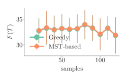
(a) Negative log-likelihood $-F({\mathcal{T}})$

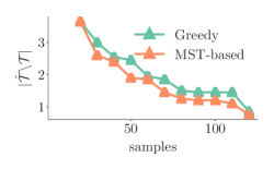
(b) Edge errors $|\hat{{\mathcal{T}}}\backslash{\mathcal{T}}|$

Figure 1: Negative log-likelihood $-F({\mathcal{T}})$ and edge errors $|\hat{{\mathcal{T}}}\backslash{\mathcal{T}}|$ achieved the greedy algorithm (Greedy; green) and a MST-based state of the art method (MST-based; orange) by Tan et al. (Tan et al., 2010). Each point corresponds to the average value across $20$ repetitions.

More applications. As pointed out by Iyer and Bilmes (2012), set functions representable as a difference between submodular functions emerged in more applications, from feature selection and discriminatively structure graphical models and neural computation to probabilistic inference. In all those applications, the inequality in Eq. 3, which must be satisfied for the functions to be $\alpha$-submodular, have a natural interpretation. For example, in feature selection with a submodular cost model for the features, it just imposes an upper bound on the penalty parameter that controls the tradeoff between the predictive power of a feature and its cost, similarly as in the case of sensor placement.

5 Experiments

In this section, our goal is to show that greedy algorithm, given by Algorithm 1, does achieve a competitive performance in practice. To this aim, we perform experiments on synthetic and real-world experiments in two of the applications introduced in Section 4, namely, tree-structure Gaussian graphical model estimation and visibility maximization in link recommendation.

5.1 Tree-structured Gaussian graphical models

Data description and experimental setup. We experiment with random trees ${\mathcal{T}}\in{\mathcal{T}}^{n}$ with $n=20$ vertices and edge weights $\Sigma_{ij}\sim U[0,10]$. We compare the performance of our estimation procedure, based on Algorithm 1, with the minimum spanning tree (MST) based estimation procedure by Tan et al. (2010), which is the state of the art method, in terms of two performance metrics: negative log-likelihood $-F({\mathcal{T}})$ and edge errors $|\hat{{\mathcal{T}}}\backslash{\mathcal{T}}|$. Here, for our estimation procedure, at each iteration of the greedy algorithm, we solve the corresponding convex problem in Eq. 13 using CVXOPT (Diamond and Boyd, 2016). Moreover, we run the estimation procedures using different number of samples and, for a fix number of samples, we repeat the experiment $20$ times to obtain reliable estimates of the performance metrics.

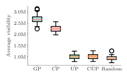
(a) $c_{i}=10$

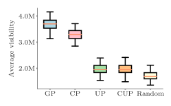
(b) $c_{i}=20$

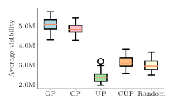
(c) $c_{i}=40$

Figure 2: Average visibility $F(\mathcal{E}_{\mathcal{B}})$ with $K=10$ achieved by the greedy algorithm (GP), the three heuristics (CP, UP, CUP) and the trivial baseline (Random) using Twitter data. The solid horizontal line shows the median visibility and the box limits correspond to the 25%-75% percentiles.

Performance. Figure 1 summarizes the results in terms of the two performance metrics, which show that both methods perform comparably, i.e., in terms of negative log-likelihood, our method beats the MST-based method slightly while, in terms of edge error, the MST-based method beats ours. The main benefit of using our greedy algorithm for this application is that, in contrast with MST, it provides optimality guarantees in terms of likelihood maximization. That being said, our goal here is to demonstrate that the greedy algorithm, which is a generic algorithm, can achieve competitive performance in a structured estimation problem for which a specialized algorithm exists.

5.2 Visibility optimization in link recommendation

Data description and experimental setup. We experiment with data gathered from Twitter as reported in previous work (Cha et al., 2010), which comprises user profiles, (directed) links between users, and (public) tweets. The follow link information is based on a snapshot taken at the time of data collection, in September 2009. Here, we focus on the tweets posted during a two month period, from July 1, 2009 to September 1, 2009, in order to be able to consider the social graph to be approximately static, sample a set $\mathcal{A}$ of $2000$ users uniformly at random, record all the tweets they posted.

We compare the performance of the greedy algorithm with a trivial baseline that picks edge uniformly at random and the same three heuristics we used in the experiments with synthetic data. Then, for $c_{i}\in\{10,20,40\}$, we repeat the following procedure $50$ times: (i) we pick uniformly at random a set $\mathcal{B}\subset\mathcal{A}$ of $80$ users as broadcasters; (ii) for each broadcaster $i$, we pick uniformly at random a set $\mathcal{H}_{i}$ of $20$ of their followers; (iii) we record all tweets not posted by broadcasters in $\mathcal{B}$ in the feeds of the users in $\mathcal{H}=\cup_{i}\mathcal{H}_{i}$; and (iv) we run the greedy algorithm, the heuristics, and the trivial baseline and record the sets $\mathcal{E}_{\mathcal{B}}=\{(i,j):i\in\mathcal{B},j\in\mathcal{H}\}$ each provides. Here, we run all methods using empirical estimates of the relevant quantities, i.e., $F$ using Eq. 57 (see Appendix C.4) and $\int_{0}^{T}\gamma(t)dt$ using maximum likelihood, computed using the tweets posted during the first month and evaluate their performance using empirical estimates of $F$ using the tweets posted during the second month.

Solution quality. Figure 2 summarizes the results by means of box plots, which show that the greedy algorithm consistently beats all heuristics and the trivial baseline. Moreover, we did experiment with other parameters settings (e.g., $|\mathcal{H}|$, $K$ and $c_{i}$) and found our method to be consistently superior to alternatives. Appendix C.5 contains additional results using synthetic data.

6 Conclusions

We have shown that a simple variation of the standard greedy algorithm offers approximation guarantees at maximizing non-submodular nondecreasing set functions under a matroid constraint. Moreover, we have identified a particular type of $\gamma$-weakly submodular functions, which we called $\xi$-submodular functions, for which the greedy algorithm offer a stronger approximation factor that is independent of the rank of the matroid. In addition, we have shown that these approximation guarantees are applicable in a variety several real-world applications, from tree-structure Gaussian graphical models and social welfare allocation to link recommendation.

Our work opens up several interesting avenues for future work. For example, a natural step would be to include the curvature of a set function in our theoretical analysis, as defined in Bian et al. (2017). Moreover, it would be very interesting to analyze the tightness of the approximation guarantees and obtaining better upper and lower bounds for $\alpha$ and $\gamma$, respectively, or even unbiased estimates, for $\xi$ and $\gamma$ in the applications we considered. Finally, it would be worth to extend our analysis to other notions of approximate submodularity (Borodin et al., 2014; Du et al., 2008; Horel and Singer, 2016; Krause et al., 2008).

Appendix A Proof of Lemma 7

Let ${\mathcal{T}}$ be the optimal set of items and ${\mathcal{S}}$ be the set of items selected by the greedy algorithm. Moreover, let $\{s_{i}\}_{i=1}^{t}$ be the items selected by the greedy algorithm in the first $t$ steps and $\{t_{i}\}_{i=1}^{q_{t}}$ be the items in $\mathcal{T}$ considered by the greedy algorithm also in the first $t$ steps in order of their consideration in the algorithm. Then, we first state the following facts, that we will use throughout the proof:

• ${\mathcal{S}}$ and ${\mathcal{T}}$ have cardinality equal to the rank of the matroid, i.e., $|{\mathcal{T}}|=|{\mathcal{S}}|=r$. This follows from the monotonicity of the function $F$.

• For any $t$, it readily follows that $q_{t}\leq t$. This follows from the proof of Theorem 9.

• There is a subset $\mathcal{R}\subseteq{\mathcal{T}}-{\mathcal{S}}_{t}$ with cardinality $|\mathcal{R}|=r-t$ such that ${\mathcal{S}}_{t}\cup\mathcal{R}\in\mathcal{I}$. This follows from the definition of a matroid.

• For all $0\leq i\leq q_{t}-1$,

  $$\rho_{s_{i+1}}({\mathcal{S}}_{i})\geq\rho_{t_{i+1}}({\mathcal{S}}_{i}).$$ (15)

  This holds because, at step $i+1$, $s_{i+1}$ and $t_{t+1}$ are not considered yet and greedy selects $s_{i+1}$. Therefore, $s_{i+1}$ must have a higher marginal gain than $t_{i+1}$.

• Let $\mathcal{R}^{\prime}={\mathcal{T}}-\{t_{1},\ldots,t_{q_{t}}\}-\mathcal{R}$, with $|\mathcal{R}^{\prime}|=t-q_{t}$. Then, for all $e\in\mathcal{R}^{\prime}$ and for all $q_{t}\leq i\leq t-1$,

  $$\rho_{s_{i+1}}({\mathcal{S}}_{i})\geq\rho_{e}({\mathcal{S}}_{i})$$ (16)

  This holds because none of the items in $\mathcal{R}^{\prime}$ are considered by the greedy algorithm in the first $t$ steps.

Now, we can use Eq. 15 and the fact that $\rho_{s_{i+1}}({\mathcal{S}}_{i})\geq\rho_{s_{j}}({\mathcal{S}}_{i})$ for $j>i$ to upper bound $\rho_{t_{i+1}}({\mathcal{S}}_{t})$ for all $0\leq i\leq q_{t}-1$:

$$\rho_{t_{i+1}}({\mathcal{S}}_{t}) \leq\rho_{t_{i+1}}({\mathcal{S}}_{t})+\sum_{j=i}^{t-1}\rho_{s_{j+1}}({\mathcal{S}}_{j})=\rho_{\{s_{i+1},...,s_{t},t_{i+1}\}}({\mathcal{S}}_{i})$$

$$\leq\frac{1}{\gamma}(\rho_{t_{i+1}}({\mathcal{S}}_{i})+\sum_{j=i}^{t-1}\rho_{s_{j+1}}({\mathcal{S}}_{i}))\leq\frac{1}{\gamma}(t+1-i)\rho_{s_{i+1}}({\mathcal{S}}_{i}).$$ (17)

Using the same technique, if we choose an arbitrary order on the elements of $\mathcal{R}^{\prime}={\mathcal{T}}-\{t_{1},\ldots,t_{q_{t}}\}-\mathcal{R}=\{e_{1},\ldots,e_{t-q_{t}}$, we can also upper bound $\rho_{e_{i+1}}({\mathcal{S}}_{t})$ for all $0\leq i\leq t-q_{t}-1$:

$$\rho_{e_{i+1}}({\mathcal{S}}_{t})\leq\frac{1}{\gamma}(t+1-q_{t}-i)\rho_{s_{q_{t}+i+1}}({\mathcal{S}}_{q_{t}+i})$$ (18)

Then, it follows from Eqs. 17 and 18 that:

$$\sum_{e\in{\mathcal{T}}-\mathcal{R}}\rho_{e}({\mathcal{S}}_{t}) \leq\frac{1}{\gamma}\sum_{i=0}^{t-1}(t+1-i)\rho_{s_{i+1}}({\mathcal{S}}_{i})=\frac{1}{\gamma}\sum_{i=0}^{t-1}(t+1-i)(F({\mathcal{S}}_{i+1})-F({\mathcal{S}}_{i}))$$

$$=\frac{1}{\gamma}\big{[}F({\mathcal{S}}_{t})+\sum_{i=0}^{t}F({\mathcal{S}}_{i})\big{]}=\frac{1}{\gamma}\big{[}1-\frac{K_{t}}{OPT}+\sum_{i=0}^{t}F({\mathcal{S}}_{i})\big{]}$$ (19)

In what follows, we will upper bound the sum in the above equation. To this end, we assume there exists $0\leq\theta\leq 1$ such that it holds that $K_{t+1}\leq(1-\theta)K_{t}$. We will specify the value of $\theta$ later. Then, it follows that $K_{t}\leq(1-\theta)^{t}OPT$ and, using that $(1-\theta)^{\frac{1}{\theta}}\leq e^{-1}$,

$$t\leq\frac{1}{\theta}\log\left(\frac{OPT}{K_{t}}\right).$$ (20)

Next, consider the geometric series $1,(1-\theta),\ldots,(1-\theta)^{\left\lfloor\frac{1}{\theta}\log\left(\frac{OPT}{K_{t}}\right)\right\rfloor}$ and notice that for $j^{*}=\left\lfloor\frac{1}{\theta}\log(\frac{OPT}{K_{t}})\right\rfloor$, it holds that

$$(1-\theta)^{j^{*}}OPT\leq(1-\theta)^{\frac{1}{\theta}\log(\frac{OPT}{K_{t}})-1}OPT\leq e^{-\log(\frac{OPT}{K_{t}})}(1-\theta)^{-1}OPT\leq\frac{K_{t}}{1-\theta}\leq K_{t-1}.$$

Then, it follows that, for each $0\leq i\leq t-1$, there exists at least a $0\leq j\leq\left\lfloor\frac{1}{\theta}\log(\frac{OPT}{K_{t}})\right\rfloor$ such that $K_{i+1}\leq(1-\theta)^{j}OPT\leq K_{i}$. Hence, we are ready to derive the upper bound we were looking for:

$$\sum_{i=0}^{t}F(S_{i}) \leq\left(\left\lfloor\frac{1}{\theta}\log(\frac{OPT}{K_{t}})\right\rfloor+1-\sum_{j=0}^{\left\lfloor\frac{1}{\theta}\log(\frac{OPT}{K_{t}})\right\rfloor}(1-\theta)^{j}\right)OPT$$

$$=\left(\left\lfloor\frac{1}{\theta}\log(\frac{OPT}{K_{t}})\right\rfloor-\sum_{j=1}^{\left\lfloor\frac{1}{\theta}\log(\frac{OPT}{K_{t}})\right\rfloor}(1-\theta)^{j}\right)OPT$$

$$\leq\left(\frac{1}{\theta}\log(\frac{OPT}{K_{t}})-(1-\theta)\frac{1-(1-\theta)^{\frac{1}{\theta}\log(\frac{OPT}{K_{t}})}}{\theta}\right)OPT$$

$$\leq\left(\frac{\log(\frac{OPT}{K_{t}})-(1-\theta)(1-\frac{K_{t}}{OPT})}{\theta}\right)OPT.$$

Moreover, using the above results, we can derive an upper bound on $K_{t}$:

$$K_{t} =OPT-F({\mathcal{S}}_{t})=F(\mathcal{T})-F({\mathcal{S}}_{t})\leq F(\mathcal{T}\cup{\mathcal{S}}_{t})-F({\mathcal{S}}_{t})\leq\rho_{{\mathcal{T}}}({\mathcal{S}}_{t})$$

$$\leq\frac{1}{\gamma}\sum_{e\in{\mathcal{T}}}\rho_{e}({\mathcal{S}}_{t})=\frac{1}{\gamma}\left(\sum_{e\in{\mathcal{T}}-\mathcal{R}}\rho_{e}({\mathcal{S}}_{t})+\sum_{e\in\mathcal{R}}\rho_{e}({\mathcal{S}}_{t})\right)$$

$$\leq\frac{1}{\gamma}\left[\frac{1}{\gamma}\left(\frac{\log(\frac{OPT}{K_{t}})-(1-\theta)(1-\frac{K_{t}}{OPT})}{\theta}+1-\frac{K_{t}}{OPT}\right)OPT+\sum_{e\in\mathcal{R}}\rho_{e}({\mathcal{S}}_{t})\right]$$

Therefore, if we define $e^{*}=\mathop{\mathrm{argmax}}_{e}\{\rho_{e}({\mathcal{S}}_{t})\}$, then

$$\rho_{e^{*}}({\mathcal{S}}_{t})\geq\frac{1}{r-t}\left[\gamma K_{t}-\frac{1}{\gamma}\left(\frac{\log(\frac{OPT}{K_{t}})-(1-\theta)(1-\frac{K_{t}}{OPT})}{\theta}+1-\frac{K_{t}}{OPT}\right)OPT\right]$$

At this point, we find the value of $\theta$ such that our assumption $K_{t+1}\leq(1-\theta)K_{t}$ holds. For that, note that it is sufficient to prove that $\rho_{e^{*}}({\mathcal{S}}_{t})\geq\theta K_{t}$. Hence, it is sufficient to prove that

$$\frac{1}{r}\left[\gamma K_{t}-\frac{1}{\gamma}\left(\frac{\log(\frac{OPT}{K_{t}})-(1-\theta)(1-\frac{K_{t}}{OPT})}{\theta}+1-\frac{K_{t}}{OPT}\right)OPT\right]\geq\theta K_{t}$$

To this end, we start by rewriting the above equation in terms of $\alpha=\frac{K_{t}}{OPT}$:

$$\frac{2}{\gamma}(1-\alpha)+\frac{1}{\gamma}\frac{\log(\frac{1}{\alpha})-1+\alpha}{\theta}+r\theta\alpha\leq\gamma\alpha.$$ (21)

In the above, it is easy to check that $\log(\frac{1}{\alpha})-1+\alpha\geq 0$. Moreover, if we fix $\alpha$, then the left hand side is minimized whenever $\theta=\sqrt{\frac{1}{\gamma}\frac{\log(\frac{1}{\alpha})-1+\alpha}{r\alpha}}$. Then, it is sufficient to prove that

$$\frac{2}{\gamma}(1-\alpha)+2\sqrt{\frac{1}{\gamma}r\alpha\left(\log\left(\frac{1}{\alpha}\right)-1+\alpha\right)}\leq\gamma\alpha$$

Moreover, since $\alpha\leq 1$ and $\log(\frac{1}{\alpha})\leq\frac{1}{\alpha}-1$, it suffices to prove that

$$\frac{1-\alpha}{\alpha\sqrt{\gamma r}}+\frac{1}{\alpha}-1\leq\frac{\gamma\sqrt{\gamma}}{2\sqrt{r}},$$

which can be rewritten as

$$\alpha\geq\frac{1}{\frac{\gamma^{2}}{2(\sqrt{\gamma r}+1)}+1}.$$

Here, we note that definition of $\theta$ depends on $\alpha$. However, if we rewrite the inequality in Eq. 21 as

$$\frac{2}{\gamma}\frac{1-\alpha}{\alpha}+\frac{\log(\frac{1}{\alpha})-1}{\gamma\theta\alpha}+\frac{1}{\gamma\theta}+r\theta\leq\gamma,$$

and realize that, for $0\leq\alpha\leq 1$, the functions $f(\alpha)=\frac{\ln(\frac{1}{\alpha})-1}{\alpha}$ and $\frac{1-\alpha}{\alpha}$ are decreasing with respect to $\alpha$, then it is easy to see that, if the above equation holds for $0\leq\alpha^{*}\leq 1$, it also holds for any $1\geq\alpha=\frac{K_{t}}{OPT}\geq\alpha^{*}$. Hence, if we define

$$\alpha^{*}=\frac{1}{\frac{\gamma^{2}}{2(\sqrt{\gamma r}+1)}+1}\quad\mbox{and}\quad\theta=\sqrt{\frac{1}{\gamma}\frac{\log(\frac{1}{\alpha^{*}})-1+\alpha}{r\alpha^{*}}},$$

we have that $\rho_{e^{*}}({\mathcal{S}}_{t})\geq\theta K_{t}$ and thus $K_{t+1}\leq K_{t}(1-\theta)$ for any step $t$ such that $\frac{K_{t}}{OPT}\geq\alpha^{*}$.

Appendix B Proof of Proposition 11

Let $\alpha\leq\sigma_{i}(\Sigma)\leq\beta$ for all $i=1,\ldots,n$. It is sufficient to prove that the curvature of the function

$$f(\Sigma)=N\log|\Sigma|-\operatorname{Tr}\left(\Sigma\sum_{i=1}^{N}x_{i}x_{i}^{T}\right)$$

in any arbitrary direction $\Sigma=Rx+C$, for $\ x\in\mathbb{R},\ R\in\mathbb{S}^{n},C\in\mathbb{S}_{++}^{n}$ is between $\alpha^{2}$ and $\beta^{2}$. Here, note that the possible directions in the space of positive definite matrices is equivalent to symmetric matrices, hence $R\in\mathbb{S}^{n}$, and we can ignore the second term in $f(\Sigma)$ since its second derivative is zero. Moreover, in the remainder, we assume that the direction matrix $R$ is normalized, i.e., $||R||_{F}=1$, where $||\cdot||_{F}$ is the Frobenius norm.

Define $g(x)=\log|Rx+C|$. First, using that $\frac{d\log|\Sigma|}{d\Sigma}=\Sigma^{-1}$, the derivative in any specific direction is given by:

$$\frac{dg}{dx}(x_{0})=\operatorname{Tr}\left(\Sigma_{0}^{-1}R\right)$$

where $\Sigma_{0}=Rx_{0}+C$. Moreover, the second derivative is readily given by

$$\frac{d^{2}g}{dx^{2}}(x_{0})=\operatorname{Tr}\left(R\frac{d\Sigma^{-1}}{dx}(x_{0})\right)=\operatorname{Tr}(R^{T}\Sigma_{0}R\Sigma_{0})=\operatorname{Tr}(R\Sigma_{0}R\Sigma_{0}).$$ (22)

Now, we compute an upper bound for $\operatorname{Tr}(R\Sigma_{0}R\Sigma_{0})$ as follows:

$$\operatorname{Tr}(R\Sigma_{0}R\Sigma_{0}) \leq\sigma_{\max}(\Sigma_{0})\operatorname{Tr}(R\Sigma_{0}R)$$ (23)

$$=\sigma_{\max}(\Sigma_{0})\operatorname{Tr}(\Sigma_{0}RR)\leq\sigma_{\max}(\Sigma_{0})^{2}\operatorname{Tr}(RR)=\sigma_{\max}(\Sigma_{0})^{2}\operatorname{Tr}(R^{T}R)$$ (24)

$$=\sigma_{\max}(\Sigma_{0})^{2}||R||_{F}^{2}=\sigma_{\max}(\Sigma_{0})^{2}\leq\beta^{2}.$$ (25)

Above, we are using the inequality $\sigma_{\text{min}}(A)Tr(B)\geq Tr(AB)\leq\sigma_{\text{max}}(A)Tr(B)$ for symmetric matrix $A$ and positive definite matrix $B$, added to the fact that the matrix $R\Sigma_{0}R$ is positive definite because $\Sigma_{0}$ is positive definite, and also $RR=R^{T}R$ is positive definite. Next, we can proceed similarly to compute a lower bound and obtain

$$\operatorname{Tr}(R\Sigma_{0}R\Sigma_{0})\geq\sigma_{\min}(\Sigma_{0})^{2}\geq\alpha^{2}.$$ (26)

The above curvature bounds readily imply that, for given matrices $X\in S^{n},Z\in D$, we have that

$$\alpha^{2}||X||_{F}^{2}\leq b(X)^{T}\frac{d^{2}f}{d(b(\Sigma))^{2}}(Z)b(X)\leq\beta^{2}||X||_{F}^{2}.$$

which is equivalent to

$$\alpha^{2}||b(X)||_{2}^{2}\leq b(X)^{T}\frac{d^{2}f}{d(b(\Sigma))^{2}}(Z)b(X)\leq\beta^{2}||b(X)||_{2}^{2},$$ (27)

where $b(K)$ is the vector representation of matrix $K$. Now, according to the mean value theorem, for $Y,Z\in D$, we know there is a matrix $T\in D$ on the line joining $Y$ and $Z$ such that

$$f(Y)=f(Z)+b(Y-Z)^{T}\frac{df}{d(b(\Sigma))}(Z)+b(Y-Z)^{T}\frac{d^{2}f}{d(b(\Sigma))^{2}}(T)b(Y-Z).$$ (28)

Applying the bounds from Eq. B completes the proof.

Appendix C Visibility optimization in link recommendation

C.1 Motivation and problem definition

Users in social networks are eager to gain new followers—to grow their audience—so that, whenever they decide to share a new story, it receives a greater amount of views, likes and shares. At the same time, users actually share quite a portion of their followers and, as a consequence, they are constantly competing with each other for attention (Backstrom et al., 2011; Gomez-Rodriguez et al., 2014), which becomes a scarce commodity of great value (Crawford, 2015). In this context, recent empirical studies have shown that stories at the top of a user’s feed are more likely to be noticed and consequently liked or shared (Hodas and Lerman, 2012; Kang and Lerman, 2015; Lerman and Hogg, 2014).

The above empirical findings have motivated the recently introduced when-to-post problem (Karimi et al., 2016; Spasojevic et al., 2015; Upadhyay et al., 2018; Zarezade et al., 2018, 2017), which aims to help a user, a broadcaster, find the best times to share stories with her followers—the times when her stories would enjoy higher visibility and would consequently elicit greater attention from her audience. While this line of work has shown great promise at helping broadcasters increase their visibility, it assumes the links between the broadcasters and their followers are given. However, these links are of great importance to the broadcaster’ visibility—they define their audience—and they are (partially) influenced by link recommendation algorithms.

The task of recommending links in social networks has a rich history in the recommender systems literature (Lü and Zhou, 2011). However, link recommendation algorithms have traditionally focused on maximizing the followers’ utility—they recommend users to follow broadcasters whose posts they may find interesting. This uncompromising focus on the utility to the followers has been called into question as social media platforms are increasingly used as news sources (Biega et al., 2018; Singh and Joachims, 2018). If we think of the broadcasters’ utility as the visibility of their posts, the following visibility optimization problem let us balance followers’ and broadcasters’ utilities.

Given a social network $\mathcal{G}=(\mathcal{V},\mathcal{E})$ and a set of candidate links $\mathcal{E}^{\prime}{}$ provided by a link recommendation algorithm, with $\mathcal{E}^{\prime}{}\cap\mathcal{E}=\emptyset$, the goal is to find a subset of these links $\mathcal{E}_{\mathcal{B}}\subseteq\mathcal{E}^{\prime}{}$ that maximize the average visibility $F(\mathcal{E}_{\mathcal{B}})$ that a set of broadcasters $\mathcal{B}$ achieve with respect to the (new) followers induced by these links, under constraints on the number of links per broadcaster, i.e.,

$$\underset{\mathcal{E}_{\mathcal{B}}\subseteq\mathcal{E}}{\text{maximize}} \quad F(\mathcal{E}_{\mathcal{B}})$$

subject to $$\quad|\{j:(i,j)\in\mathcal{E}_{\mathcal{B}}\}|\leq c_{i},\quad\forall i\in\mathcal{B}$$ (29)

where we can express the constraints as $|\mathcal{B}|$ partition matroid constraints, i.e., $\mathcal{I}=\{\mathcal{E}_{\mathcal{B}}|\mathcal{E}_{\mathcal{B}}\subseteq\mathcal{E},\,|\mathcal{E}_{\mathcal{B}}\cap\mathcal{E}_{i,:}^{\prime}{}|\leq c_{i}\,\forall i\in\mathcal{B}\}$, where $\mathcal{E}_{i,:}^{\prime}{}$ denotes the ground set of candidate links from broadcaster $i$, and $c_{i}$ is the maximum number of links that broadcaster $i$ can afford. In the following sections, we denote the set of broadcasters and followers corresponding to the set of candidate links $\mathcal{E}^{\prime}$ as $\mathcal{V}^{\prime}\subseteq\mathcal{V}$.

C.2 Definition and computation of visibility

In this section, we formally define the measure of visibility and, using previous work (Karimi et al., 2016; Zarezade et al., 2018, 2017), derive a relationship between this visibility measure and the intensity (or rates) at which broadcaster post stories and followers receive stories in their feeds. Refer to De et al. (2019) for an introduction to the theory of temporal point processes, which is used throughout the section.

Definition of visibility. Given a broadcaster $i$ and one of her followers $j$, let $r(t,i,j)$ be the number of stories posted by $i$ that are among the top $K$ positions of $j$’s feed at time $t$ and, for simplicity, assume each user’s feed ranks stories in inverse chronological order, as in previous work (Karimi et al., 2016; Zarezade et al., 2018, 2017). Then, given an observation time window $[t_{0},t_{f}]$ and a deterministic sequence of broadcasting events, define the deterministic top $K$ visibility of broadcaster $i$ with respect to follower $j$ as

$${\mathcal{T}}(i,j):=\int_{t_{0}}^{t_{f}}r(t,i,j)dt,$$ (30)

which is the number of stories posted by $i$’s that are among the top $K$ positions of $j$’s feed over time. However, since the sequence of broadcasting events are generated from stochastic processes, consider instead the expected value of the top $K$ visibility instead, i.e.,

$$\mathcal{U}(i,j)=\mathbb{E}\left[{\mathcal{T}}(i,j)\right]=\int_{t_{0}}^{t_{f}}\mathbb{E}\left[r(t,i,j)\right]dt.$$ (31)

Then, by definition, it readily follows that

$$\mathbb{E}\left[r(t,i,j)\right]=\sum_{k=1}^{K}g_{k}(t,i,j),$$ (32)

where $g_{k}(t,i,j)$ is the probability that a story posted by broadcaster $i$ is at position $k$ of follower $j$’s feed at time $t$. Finally, given a set of broadcasters $\mathcal{B}$ and a set of links $\mathcal{E}_{\mathcal{B}}$, define the average top $K$ visibility (or, in short, average visibility) of the broadcasters with respect to the followers induced by the links as

$$F(\mathcal{E}_{\mathcal{B}}):=\sum_{j\in\mathcal{V}^{\prime}{}}F(\mathcal{E}_{\mathcal{B}},j),$$ (33)

where, with an overload of notation,

$$F(\mathcal{E}_{\mathcal{B}},j):=\sum_{i\in\mathcal{B}\,:\,(i,j)\in\mathcal{E}_{\mathcal{B}}}\mathcal{U}(i,j).$$

Here, note that, by using the linearity of expectation, we can also write $F(\mathcal{E}_{\mathcal{B}},j)$ in terms of the number of stories $r(t,\mathcal{E}_{\mathcal{B}},j)$ posted by the broadcasters that are among the top $K$ positions of user $j$’s feed at time $t$ and the probability $g_{k}(t,\mathcal{E}_{\mathcal{B}},j)$ that a story posted the broadcasters is at position $k$ of user $j$’s feed at time $t$, i.e.,

$$F(\mathcal{E}_{\mathcal{B}},j)=\int_{t_{0}}^{t_{f}}\mathbb{E}\left[r(t,\mathcal{E}_{\mathcal{B}},j)\right]=\int_{t_{0}}^{t_{f}}\sum_{k=1}^{K}g_{k}(t,\mathcal{E}_{\mathcal{B}},j),$$ (34)

where we have again overloaded the notation for simplicity.

Computation of visibility. Following a similar procedure as in Zarezade et al. (2018, 2017), we can find a closed form expression for the probability $g_{k}(t)=g_{k}(t,i,j)$ that one story from a broadcaster $i$ with intensity $\mu(t)$ is at the top of a follower $j$’s feed with intensity $\gamma(t)$ at time $t$:

Lemma 14.

Given a broadcaster with intensity $\mu(t)$ and one of her followers with feed intensity due to other broadcasters $\gamma(t)$, the probability $g_{k}(t)$ that a story posted by the broadcaster is at position $k$ of the follower’s feed at time $t$ is given by

$$g_{k}(t)=\int_{0}^{t}\frac{J^{k-1}(\mu+\gamma,\tau,t)}{(k-1)!}e^{-J(\mu+\gamma,\tau,t)}\mu(\tau)d\tau,$$ (35)

where $J(\lambda,\tau,t)=\int_{\tau}^{t}\lambda(x)dx$.

Then, if we plug Eq. 35 into Eq. 32 with $r(t)=r(t,i,j)$, we obtain

$$\mathbb{E}\left[r(t)\right]=\int_{0}^{t}\left[\sum_{k=1}^{K}\frac{J^{k-1}(\mu+\gamma,\tau,t)}{(k-1)!}\right]e^{-J(\mu+\gamma,\tau,t)}\mu(\tau)d\tau=(K-1)!\int_{0}^{t}\Gamma\left(K,J(\mu+\gamma,\tau,t)\right)\mu(\tau)d\tau,$$

where $\Gamma(K,x)$ is the incomplete gamma function. Using that $\frac{dJ(\mu+\gamma,\tau,t)}{d\tau}=-(\mu(\tau)+\gamma(\tau))$, we can simplify the above expression into

$$\mathbb{E}\left[r(t)\right]=-G(J(\mu+\gamma,t,t))+G(J(\mu+\gamma,0,t))-\frac{1}{(K-1)!}\int_{0}^{t}\Gamma(K,J(\mu+\gamma,\tau,t))\gamma(\tau){d\tau},$$

where $G(x)=-\sum_{i=0}^{K-1}(K-i)\frac{x^{i}}{i!}e^{-x}$ is the anti-derivative of $\Gamma(K,x)$. Then, using that $J(\mu+\gamma,t,t)=0$, $G(0)=-K$ and

$$J(\mu+\gamma,0,t)=\int_{0}^{t}\mu(x)+\gamma(x)dx,$$

it follows that

$$\mathbb{E}\left[r(t)\right]=K+G\left(\int_{0}^{t}\mu(x)+\gamma(x)dx\right)-\frac{1}{(K-1)!}\int_{0}^{t}\Gamma(K,J(\mu+\gamma,\tau,t))\gamma(\tau){d\tau}.$$ (36)

Finally, if we plug Eq. 36 into Eq. 31, we obtain an expression for the average top $K$ visibility of broadcaster $i$ with respect to follower $j$ in terms of the intensity functions $\mu(t)$ and $\gamma(t)$ characterizing the broadcaster and the follower, respectively:

$$\mathcal{U}(i,j)=K(t_{f}-t_{0})+\int_{t_{0}}^{t_{f}}G\left(\int_{0}^{t}\mu(x)+\gamma(x)dx\right)dt-\frac{1}{(K-1)!}\int_{t_{0}}^{t_{f}}\int_{0}^{t}\Gamma(K,J(\mu+\gamma,\tau,t))\gamma(\tau){d\tau}dt.$$ (37)

Given a social network $\mathcal{G}=(\mathcal{V},\mathcal{E})$, a set of candidate links $\mathcal{E}^{\prime}{}$ provided by a link recommendation algorithm, with $\mathcal{E}^{\prime}{}\cap\mathcal{E}=\emptyset$, and a subset of links $\mathcal{E}_{\mathcal{B}}\subseteq\mathcal{E}^{\prime}{}$, we can proceed similarly as in the case of one links and show that:

• The probability $g_{k}(t,\mathcal{E}_{\mathcal{B}},j)$ that a story posted by the broadcasters user $j$ gains due to the links $\mathcal{E}_{\mathcal{B}}$ is at position $k$ of her feed at time $t$ is given by Eq. 35 with $\gamma(t)=\gamma_{j\,|\,\mathcal{E}}(t)$, where $\gamma_{j\,|\,\mathcal{E}}(t)$ denotes the intensity at which follower $j$ receives stories in her feed due to other broadcasters she follows, and $\mu(t)=\sum_{i\in\mathcal{B}\,:\,(i,j)\in\mathcal{E}_{\mathcal{B}}}\mu_{i}(t)$.

• The average visibility $\mathcal{U}(\mathcal{E}_{\mathcal{B}},j)$ with respect to user $j$ of the broadcasters this user gains due to the links $\mathcal{E}_{\mathcal{B}}$ is given by Eq. 37 with $\gamma(t)=\gamma_{j\,|\,\mathcal{E}}(t)$ and $\mu(t)=\sum_{i\in\mathcal{B}\,:\,(i,j)\in\mathcal{E}_{\mathcal{B}}}\mu_{i}(t)$.

Finally, the above results allow us to write $F(\mathcal{E}_{\mathcal{B}})$, given by Eq. 33, in terms of intensity functions characterizing the broadcasters and the feeds, as we were aiming for.

C.3 $\alpha$-submodularity of the visibility

Given a social network $\mathcal{G}=(\mathcal{V},\mathcal{E})$, let $\mathcal{E}_{\mathcal{B}}\subseteq\mathcal{E}^{\prime}{}$ be a set of candidate links, with $\mathcal{E}^{\prime}{}\cap\mathcal{E}=\emptyset$, $\{\mu_{i}(t)\}_{i\in\mathcal{B}}$ be the intensities of a set of broadcasters $\mathcal{B}\subseteq\mathcal{V}$, and $\{\gamma_{i\,|\,\mathcal{E}}(t)\}_{i\in\mathcal{V}}$ be the users’ feed intensities due to the broadcasters induced by the links $\mathcal{E}$. Define $\inf(\lambda)=\inf\{\lambda(t)\mid t\in(t_{0},t_{f})\}$, $\sup(\lambda)=\sup\{\lambda(t)\mid t\in(t_{0},t_{f})\}$ and assume that:

• All intensities are bounded above, i.e., $\sup(\mu_{i})\leq c_{1},\,\forall i\in\mathcal{B}$ and $\sup(\gamma_{i\,|\,\mathcal{E}})\leq c_{1},\,\forall i\in\mathcal{V}$ with $0<c_{1}<\infty$.

• The users’ feed intensities due to the broadcasters induced by the links $\mathcal{E}$ are bounded below, i.e., $\inf(\gamma_{i\,|\,\mathcal{E}})\geq c_{2},\,\forall i\in\mathcal{V}$ with $0<c_{2}\leq c_{1}$.

Note that these assumptions are natural in most practical scenarios—the first assumption is satisfied if broadcasters post a finite number of stories per unit of time and the second assumption is satisfied if, at any time, there is always a nonzero probability that a user’s feed receives a post from the other broadcasters. Moreover, under these assumptions, it readily follows that, for any set $\mathcal{E}_{\mathcal{B}}$, the feed intensities $\gamma_{i}(t)$ are $\xi$-bounded, i.e., $\sup(\gamma_{i})\leq\xi\inf(\gamma_{i})$, with $\xi\leq\frac{c_{1}}{c_{2}}(1+|\mathcal{E}^{\prime}{}_{:,i}|)$, where $\mathcal{E}_{i,:}^{\prime}{}$ denotes the ground set of candidate links from broadcaster $i$.

Then, we can characterize the generalized curvature $\alpha$ of the average visibility $F(\mathcal{E}_{\mathcal{B}})$ using the following Theorem:

Theorem 15.

Suppose that, for any set $\mathcal{E}_{\mathcal{B}}\subseteq\mathcal{E}^{\prime}{}$, the feed intensities $\gamma_{i}(t)$ are $\xi$-bounded and, for each follower $j$,

$$\int_{0}^{t_{0}}\gamma_{j\,|\,\mathcal{E}}(x)dx\geq K-1+\zeta\sqrt{K-1},\,\forall j\in\mathcal{V}$$ (38)

for some $\zeta>0$, which simply states that $t_{0}$ is large enough so that the expected number of stories posted by the broadcasters induced by $\mathcal{E}$ by $t_{0}$ in each follower’s feed is greater than the RHS. Then, the generalized curvature $\alpha$ of the average visibility $F(\mathcal{E}_{\mathcal{B}})$, defined by Eq. 33, satisfies that

$$\alpha\leq\alpha^{*}=1-\frac{1}{\xi\left(\frac{6.154e^{2}}{1-\frac{4e^{\frac{7}{4}}}{\zeta}}\xi\sqrt{K}+1\right)}.$$ (39)

Corollary 16.

The generalized curvature of the average visibility $F(\mathcal{E}_{\mathcal{B}})$ is given by $\alpha\approx 1-\Omega\left(\frac{1}{\xi^{2}\sqrt{K}}\right)$.

Moreover, if we assume that, at each time $t$, the intensity function $\mu_{i}(t)$ of each broadcaster is lower than a fraction of each of her follower’s feed intensities then we can tighten upper bound $\alpha^{*}$ given by Theorem 15 using the following Theorem and Corollary.

Theorem 17.

Suppose the conditions in Theorem 15 hold and, in addition,

$$\mu_{i}(t)\leq\frac{\gamma_{j\,|\,\mathcal{E}}(t)}{\rho\sqrt{K-1}},\quad\forall t\in[t_{0},t_{f}],\forall i\in\mathcal{B},\forall j\in\mathcal{V}^{\prime}{},$$ (40)

where $\rho>0$. Then, the generalized curvature $\alpha$ of the average visibility $F(\mathcal{E}_{\mathcal{B}})$ satisfies that

$$\alpha\leq\alpha^{*}=1-\frac{1}{\alpha\left(\frac{2e^{\frac{7}{4}}}{(1-\frac{4e^{\frac{7}{4}}}{\zeta})\min\{\rho,1\}e^{-\frac{1}{\rho^{2}}}}\xi+1\right)}.$$ (41)

Note that we can always find a constant $\rho>0$ so that Eq. 41 is satisfied, however, the term $\min\{\rho,1\}e^{-\frac{1}{\rho^{2}}}$ will decrease drastically when $\rho\geq 1$. Finally, by combining Theorems 15 and Theorem 17, we obtain Proposition 12 in the main paper.

Proof sketch of Theorems 15 and 17. To bound the generalized curvature of the average visibility $F(\mathcal{E}_{\mathcal{B}})$, defined by Eq. 33, we have to provide a $\alpha$ satisfying the inequality in Eq. 2. The following Lemma lets us omit several sums and integrations Eq. 33 depends on while deriving a bound for the generalized curvature.

Lemma 18.

Let $\{F_{\sigma}\}_{\sigma\in\wp}$ be a family of set functions $F_{\sigma}:\mathcal{W}\rightarrow\mathbb{R}$ parametrized by $\sigma$, such that for each fixed $\sigma\in\wp$, $F_{\sigma}$ is a set function with generalized curvature $\alpha_{\sigma}\leq\alpha^{*}$. Then, the following statements hold:

• Suppose $\wp=(a,b)\subseteq\mathbb{R}$ and $\tilde{F}(S)=\int_{a}^{b}F_{\sigma}(S)\,d\sigma$ for every subset $S\subseteq\mathcal{V}$ and the integral always exists. Then, $\tilde{F}$ has generalized curvature $\alpha\leq\alpha^{*}$.

• Suppose $\wp$ is a discrete set and $\tilde{F}(S)=\sum_{\sigma\in\wp}F_{\sigma}(S)$. Then, $\tilde{F}$ has generalized curvature $\alpha\leq\alpha^{*}$.

For both cases introduced, if for each $\sigma$, $F_{\sigma}$ is submodular, then $F$ is submodular as well.

Proof.

By the definition of generalized curvature, $\forall v\in\mathcal{W}$, $A\subseteq B$, $\forall\sigma$:

$$F_{\sigma}(A\cup\{v\})-F_{\sigma}(A)\geq(1-\alpha_{\sigma})(F_{\sigma}(B\cup\{v\})-F_{\sigma}(B))\geq(1-\alpha^{*})(F_{\sigma}(B\cup\{v\})-F_{\sigma}(B)).$$ (42)

By integrating over both sides of Eq. 42 over $\sigma$ we get

$$F(A\cup\{v\})-F(A)\geq(1-\alpha_{\sigma})(F(B\cup\{v\})-F(B))\geq(1-\alpha^{*})(F(B\cup\{v\})-F(B)),$$

which proves $\alpha\leq\alpha^{*}$. The proof for the second part follows the same way by summing over $\sigma\in\wp$. ∎

More specifically, using the first statement of Lemma 18, in order to obtain an upper bound for the generalized curvature for $F(\mathcal{E}_{\mathcal{B}})$, it is sufficient to obtain an upper bound for each $\mathcal{U}(\mathcal{E}_{\mathcal{B}},j)$, which is a summation of three terms, as given by Eq. 37. The first term, $K(t_{f}-t_{0})$, is a constant and does not appear in the marginal gains $\{\rho_{e}\}_{e\in\mathcal{E}_{\mathcal{B}}}$, therefore, it does not affect the generalized curvature. Using the second statement of Lemma 18, it is sufficient to obtain an upper bound for the generalized curvature of the second and third term separately.

The second term is the integration of the function $G$ in the time interval $(t_{0},t_{f})$. Therefore, using the first statement of Lemma 18, it is sufficient to obtain an upper bound for the generalized curvature of the function $G$ for any $t\in[t_{0},t_{f}]$. Here, note that the function $G$ only depends on the links pointing at follower $j$, therefore, its ground set $\mathcal{E}_{:,j}^{\prime}{}$ is the ground set of candidate links from the broadcasters to $j$. Next, we will use the following Lemma to show that $G$ is a submodular function and thus its generalized curvature is $\alpha=0$:

Lemma 19.

Let $G({\mathcal{S}})=f(c+F({\mathcal{S}}))$ be a nonnegative set function, where $f$ is a concave function over $\mathbb{R}^{+}$, $F$ is a nonnegative modular function, and $c$ is a nonnegative constant. Then, $G$ is submodular.

Proof.

According to Lemma 21 and by using the property of modular functions, for $A\subseteq B$, it follows that

$$G(B\cup\{v\})-G(B) =f(c+F(B\cup\{v\}))-f(c+F(B))$$

$$=f(c+F(B\setminus A)+F(A\cup\{v\}))-f(c+F(B\setminus A)+F(A))$$

$$\leq f(c+F(A\cup\{v\}))-f(c+F(A))=G(A\cup\{v\})-G(A).$$

∎

Moreover, the parameter of the function $G$, i.e.,

$$\int_{0}^{t}\sum_{i\in\mathcal{B}\,:\,(i,j)\in\mathcal{E}_{\mathcal{B}}}\mu_{i}(x)+\gamma_{j\,|\,\mathcal{E}}(x)dx,$$

for a fixed $t$, it is a sum of a modular function over the groundset $\mathcal{E}_{:,j}^{\prime}{}$ of candidate links from the broadcasters to $j$ and a constant. Moreover, $G$ is concave in $\mathbb{R}^{+}$ since $G^{\prime}(x)=-\frac{x^{K-1}e^{-x}}{(K-1)!}\leq 0$. Therefore, we can use Lemma 19 to conclude that the second term is submodular over the groundset $\mathcal{E}_{:,j}^{\prime}{}$. This means that an upper bound for the generalized curvature of the third term in Eq. 37 will be an upper bround for the generalized curvature of $F(\mathcal{E}_{\mathcal{B}})$, on the grounds of Lemma 18.

To upper bound the generalized curvature of the third term, using the second statement of Lemma 18, it is sufficient to provide an upper bound on the generalized curvature of

$$-\int_{0}^{t}\Gamma(K,J(\mu+\gamma,\tau,t))\gamma(\tau){d\tau}:=\mathcal{P}_{j}(\mathcal{E}_{\mathcal{B}}),$$ (43)

where $\mu(\tau)=\sum_{i\in\mathcal{B}\,:\,(i,j)\in\mathcal{E}_{\mathcal{B}}}\mu_{i}(\tau)$ and $\gamma(\tau)=\gamma_{j\,|\,\mathcal{E}}(\tau)$. Here, note that the above function depends on the candidate links $\mathcal{E}_{\mathcal{B}}$ through $\mu(\tau)$. Moreover, the function $J(\mu+\gamma,\tau,t)$ is the sum of a modular function over the ground set $\mathcal{E}_{:,j}^{\prime}{}$ of candidate links from the broadcasters to $j$ and a constant. Thus, if $-\Gamma(K,x)$ was concave for $x\in\mathbb{R}^{+}$, then we could combine the second statement of Lemma 18 and Lemma 19 to conclude that $\mathcal{P}_{j}(\mathcal{E}_{\mathcal{B}})$ is submodular over $\mathcal{E}_{:,j}^{\prime}{}$. Unfortunately, $-\Gamma$ is convex on $(0,K-1)$ and concave on $(K-1,\infty)$.

With this in mind, we define the time point $0\leq\tau_{0}=\tau_{0}(\mu+\gamma,t)\leq t$ such that $J(\mu+\gamma,\tau_{0},t)=K-1$, which will allow us to analyze the domains $(0,K-1)$ and $(K-1,\infty)$ separately. Here, note that such $\tau_{0}$ exists because $J(\mu+\gamma,t,t)=0$,

$$J(\mu+\gamma,0,t) =\int_{0}^{t}\sum_{i\in\mathcal{B}\,:\,(i,j)\in\mathcal{E}_{\mathcal{B}}}\mu_{i}(x)+\gamma_{j\,|\,\mathcal{E}}(x)dx\geq\int_{0}^{t}\gamma_{j\,|\,\mathcal{E}}(x)dx\geq\int_{0}^{t_{0}}\gamma_{j\,|\,\mathcal{E}}(x)dx$$

$$\geq K-1\!\!\ +\zeta\sqrt{K-1}\!\!\geq K-1,$$

using Eq. 38 in Theorem 15, and the fact that $J(\mu+\gamma,\tau,t)$ is a continuous (nonincreasing) function with respect to $\tau$.

The following Lemma (proven in Appendix C.3.1) introduces a key inequality to derive an upper bound on the generalized curvature of $\mathcal{P}(\mathcal{E}_{\mathcal{B}})$.

Lemma 20.

Given a social network $\mathcal{G}=(\mathcal{V},\mathcal{E})$. Let $\mathcal{E}_{\mathcal{B}},\tilde{\mathcal{E}}_{\mathcal{B}}$ be two possible sets of candidate links from a set of broadcasters $\mathcal{B}$, such that $\mathcal{E}_{\mathcal{B}}\subseteq\tilde{\mathcal{E}}_{\mathcal{B}}$ and $\tilde{\mathcal{E}}_{\mathcal{B}}\cap\mathcal{E}=\emptyset$, $j\in\mathcal{V}$ a given user with feed intensity $\gamma_{j\,|\,\mathcal{E}}(t)=\gamma(t)$ due to broadcasters induced by $\mathcal{E}$,

$$\mu(t)=\sum_{i\in\mathcal{B}:(i,j)\in\mathcal{E}_{\mathcal{B}}}\mu_{i}(t)\quad\mbox{and}\quad\tilde{\mu}(t)=\sum_{i\in\mathcal{B}:(i,j)\in\tilde{\mathcal{E}}_{\mathcal{B}}}\mu_{i}(t)$$

be the intensities induced by the links $\mathcal{E}_{\mathcal{B}}$ and $\tilde{\mathcal{E}}_{\mathcal{B}}$, respectively, in user $j$’s feed, and assume the intensities $\gamma(t)$, $\gamma(t)+\mu(t)$ and $\gamma(t)+\tilde{\mu}(t)$ to be $\xi$-bounded. Consider a broadcaster $i\in\mathcal{B}$ with intensity $\mu_{i}(t)=\lambda(t)$, such that $(i,j)\notin\tilde{\mathcal{E}}_{\mathcal{B}}$. Then, under conditions of Theorem 15, it holds that

$$\theta \left[\int_{0}^{t}\Gamma(K,J(\mu+\gamma,\tau,t))d\tau-\int_{0}^{t}\Gamma(K,J(\mu+\gamma+\lambda,\tau,t)){d\tau}\right]$$

$$\geq \int_{0}^{t}\Gamma(K,J(\tilde{\mu}+\gamma,\tau,t))d\tau-\int_{0}^{t}\Gamma(K,J(\tilde{\mu}+\gamma+\lambda,\tau,t)){d\tau},$$ (44)

where

$$\theta=\theta_{1}=\frac{6.154e^{2}}{1-\frac{4e^{\frac{7}{4}}}{\zeta}}\xi\sqrt{K}+1.$$ (45)

Moreover, under extra condition of Theorem 17, Eq. 44 also holds for

$$\theta=\theta_{2}=\frac{2e^{\frac{7}{4}}}{(1-\frac{4e^{\frac{7}{4}}}{\zeta})\min\{\rho,1\}e^{-\frac{1}{\rho^{2}}}}\xi+1.$$ (46)

With the above Lemma, we are now ready to derive an upper bound on the generalized curvature of $\mathcal{P}_{j}(\mathcal{E}_{\mathcal{B}})$. Consider the same definitions and assumptions as in the above Lemma. Then,

$$\mathcal{P}_{j}(\mathcal{E}_{\mathcal{B}}\cup\{(i,j)\})-\mathcal{P}_{j}(\mathcal{E}_{\mathcal{B}}) =\int_{0}^{t}\big{(}\Gamma(K,J(\mu+\gamma,\tau,t))-\Gamma(K,J(\mu+\gamma+\lambda,\tau,t))\big{)}\gamma(\tau)d\tau$$

$$\geq\inf(\gamma)\int_{0}^{t}\big{(}\Gamma(K,J(\mu+\gamma,\tau,t))-\Gamma(K,J(\mu+\gamma+\lambda,\tau,t))\big{)}d\tau$$

$$\stackrel{{\scriptstyle(a)}}{{\geq}}\frac{\inf(\gamma)}{\theta}\int_{0}^{t}\big{(}\Gamma(K,J(\tilde{\mu}+\gamma,\tau,t))-\Gamma(K,J(\tilde{\mu}+\gamma+\lambda,\tau,t))\big{)}d\tau$$

$$\geq\frac{\inf(\gamma)}{\theta\sup(\gamma)}\int_{0}^{t}\big{(}\Gamma(K,J(\tilde{\mu}+\gamma,\tau,t))-\Gamma(K,J(\tilde{\mu}+\gamma+\lambda,\tau,t))\big{)}\gamma(\tau)d\tau$$

$$\stackrel{{\scriptstyle(b)}}{{\geq}}\frac{1}{\theta\xi}\int_{0}^{t}\big{(}\Gamma(K,J(\tilde{\mu}+\gamma,\tau,t))-\Gamma(K,J(\tilde{\mu}+\gamma+\lambda,\tau,t))\big{)}\gamma(\tau)d\tau$$

$$=(1-\alpha)\big{(}\mathcal{P}_{j}(\tilde{\mathcal{E}}_{\mathcal{B}}\cup\{(i,j)\})-\mathcal{P}_{j}(\tilde{\mathcal{E}}_{\mathcal{B}})\big{)},$$

where (a) follows from the Lemma and (b) follows from the $\xi$-boundedness of $\gamma$. This result implies that $\alpha$, defined in Eq. 39 or Eq. 41, is an upper bound on the generalized curvature of $\mathcal{P}_{j}(\mathcal{E}_{\mathcal{B}})$, thereby, it is an upper bound on that of $F(\mathcal{E}_{\mathcal{B}})$ as well.

C.3.1 Proof of Lemma 20

We start by subtracting the left hand side (LHS) and the right hand side (RHS) of Eq. 44 and splitting the integration interval into subintervals $(0,\tau_{0})$ and $(\tau_{0},t)$ with $\tau_{0}=\tau_{0}(\mu+\gamma,t)$ such that $J(\mu+\gamma,\tau_{0},t)=K-1$:

$$LHS-RHS=\Delta(0,\tau_{0})+\Delta(\tau_{0},t),$$

where

$$\Delta(a,b)= \theta\left[\int_{a}^{b}\Gamma(K,J(\mu+\gamma,\tau,t))d\tau-\int_{a}^{b}\Gamma(K,J(\mu+\gamma+\lambda,\tau,t)){d\tau}\right]$$

$$-\left[\int_{a}^{b}\Gamma(K,J(\tilde{\mu}+\gamma,\tau,t))d\tau-\int_{a}^{b}\Gamma(K,J(\tilde{\mu}+\gamma+\lambda,\tau,t)){d\tau}\right].$$

For $\tau\leq\tau_{0}$, we have that $J(\mu+\gamma,\tau,t)\geq K-1$ using the fact that $J(\mu+\gamma,\tau,t)$ is nonincreasing with respect to $\tau$. Moreover, note that the intensity $\tilde{\mu}(t)$ is the summation of $\mu(t)$ with the intensity due to broadcasters $\tilde{\mathcal{E}}_{\mathcal{B}}\backslash\mathcal{E}_{\mathcal{B}}$. Therefore,

$$J(\tilde{\mu}+\gamma,\tau,t)=\int_{\tau}^{t}\tilde{\mu}(x)+\gamma(x)dx\geq\int_{\tau}^{t}\mu(x)+\gamma(x)dx=J(\mu+\gamma,\tau,t)\geq K-1.$$

In a similar way, we can conclude that

$$J(\mu+\gamma+\lambda,\tau,t),\,J(\tilde{\mu}+\gamma+\lambda,\tau,t)\geq K-1.$$

Then, using that the composite function $\Gamma(K,J(\mu+\gamma+\lambda,\tau,t))$ is convex in $J$ for $\tau\leq\tau_{0}$ and, for any convex function $f$, $x\geq x^{\prime}$, and $y\geq 0$, $f(x)-f(x+y)\leq f(x^{\prime})-f(x^{\prime}+y)$ (refer to Lemma 21), it follows that

$$\Gamma(K,J(\mu+\gamma,\tau,t))-\Gamma(K,J(\mu+\gamma+\lambda,\tau,t))\geq\Gamma(K,J(\tilde{\mu}+\gamma,\tau,t))-\Gamma(K,J(\tilde{\mu}+\gamma+\lambda,\tau,t)).$$

Next, we can integrate the above equation and obtain that

$$\int_{0}^{\tau_{0}} \Gamma(K,J(\mu+\gamma,\tau,t))d\tau-\int_{0}^{\tau_{0}}\Gamma(K,J(\mu+\gamma+\lambda,\tau,t)){d\tau}$$

$$\geq\int_{0}^{\tau_{0}}\Gamma(K,J(\tilde{\mu}+\gamma,\tau,t))d\tau-\int_{0}^{\tau_{0}}\Gamma(K,J(\tilde{\mu}+\gamma+\lambda,\tau,t)){d\tau},$$

which implies

$$\Delta(0,\tau_{0})\geq(\theta-1)\big{(}\int_{0}^{\tau_{0}}\Gamma(K,J(\mu+\gamma,\tau,t))d\tau-\int_{0}^{\tau_{0}} \Gamma(K,J(\mu+\gamma+\lambda,\tau,t))d\tau\big{)}\geq 0,$$ (47)

using that $\Gamma(K,x)$ is nonincreasing with respect to $x$ and $\theta>1$. Unfortunately, $\Delta(\tau_{0},t)$ can be negative. However, in the following, we will show that $\Delta(\tau_{0},t)\geq-\Delta(0,\tau_{0})$.

Let $d=J(\lambda,\tau_{0},t)$. First, note that, for $\tau\leq\tau_{0}$, $J(\lambda,\tau,t)\geq J(\lambda,\tau_{0},t)=d$. Then, starting from Eq. 47, we have that

$$\Delta(0,\tau_{0}) \geq(\theta-1)\int_{J(\mu+\gamma,0,t)}^{J(\mu+\gamma,\tau_{0},t)}\big{[}\Gamma(K,J(\mu+\gamma,\tau,t))-\Gamma(K,J(\mu+\gamma+\lambda\tau,t))\big{]}\frac{d\tau}{dJ(\mu+\gamma,\tau,t)}dJ(\mu+\gamma,\tau,t)$$

$$=(\theta-1)\int_{K-1}^{J(\mu+\gamma,0,t)}\frac{1}{\mu(\tau)+\gamma(\tau)}\big{[}\Gamma(K,J(\mu+\gamma,\tau,t))-\Gamma(K,J(\mu+\gamma+\lambda,\tau,t))\big{]}dJ(\mu+\gamma,\tau,t)$$

$$\geq\frac{\theta-1}{\sup(\mu+\gamma)}\int_{K-1}^{J(\mu+\gamma,0,t)}\big{[}\Gamma(K,J(\mu+\gamma,\tau,t))-\Gamma(K,J(\mu+\gamma,\tau,t)+d)\big{]}dJ(\mu+\gamma,\tau,t)$$

$$=\frac{\theta-1}{\sup(\mu+\gamma)}\int_{K-1}^{J(\mu+\gamma,0,t)}\big{[}\Gamma(K,x)-\Gamma(K,x+d)\big{]}dx$$

$$=\frac{\theta-1}{\sup(\mu+\gamma)}\big{[}\int_{K-1}^{J(\mu+\gamma,0,t)}\Gamma(K,x)dx-\int_{K-1+d}^{J(\mu+\gamma,0,t)+d}\!\!\!\!\!\!\!\!\!\Gamma(K,x)dx\big{]}$$

$$=\frac{\theta-1}{\sup(\mu+\gamma)}\big{[}\int_{K-1}^{K-1+d}\Gamma(K,x)dx-\int_{J_{s}^{t}(0)}^{J_{s}^{t}(0)+d}\Gamma(K,x)dx\big{]}$$

Next, we can use the first statement of Lemma 22 (refer to Appendix C.3.2) to bound the second integration term above and obtain that

$$\Delta(0,\tau_{0})\geq\frac{\theta-1}{\sup(s)}\left(1-\frac{4e^{\frac{7}{4}}}{\zeta}\right)\int_{K-1}^{K-1+d}\Gamma(K,x)dx.$$ (48)

Second, note that, for $\tau\geq\tau_{0}$, $J(\lambda,\tau,t)\leq d$. Then, we have that

$$\begin{split}\Delta(\tau_{0},t)&\geq-\left(\int_{\tau_{0}}^{t}\Gamma(K,J(\tilde{\mu}+\gamma,\tau,t))d\tau-\int_{\tau_{0}}^{t}\Gamma(K,J(\tilde{\mu}+\gamma+\lambda,\tau,t)){d\tau}\right)\\ &=-\int_{J(\tilde{\mu}+\gamma,\tau_{0},t)}^{J(\tilde{\mu}+\gamma,t,t)}\big{[}\Gamma(K,J(\tilde{\mu}+\gamma,\tau,t))\\ &\qquad-\Gamma(K,J(\tilde{\mu}+\gamma+\lambda,\tau,t))\big{]}\frac{d\tau}{dJ(\tilde{\mu}+\gamma,\tau,t)}dJ(\tilde{\mu}+\gamma,\tau,t)\\ &=-\int_{0}^{J(\tilde{\mu}+\gamma,\tau_{0},t)}\frac{1}{\tilde{\mu}(\tau)+\gamma(\tau)}\big{[}\Gamma(K,J(\tilde{\mu}+\gamma,\tau,t))\\ &\qquad-\Gamma(K,J(\tilde{\mu}+\gamma+\lambda,\tau,t))\big{]}dJ(\tilde{\mu}+\gamma,\tau,t)\\ &\geq-\frac{1}{\inf(\tilde{\mu}+\gamma)}\int_{0}^{J(\tilde{\mu}+\gamma,\tau_{0},t)}\big{(}\Gamma(K,x)-\Gamma(K,x+d)\big{)}dx\\ &\geq-\frac{1}{\inf(\tilde{\mu}+\gamma)}\int_{0}^{\infty}\big{(}\Gamma(K,x)-\Gamma(K,x+d)\big{)}dx\\ &=-\frac{1}{\inf(\tilde{\mu}+\gamma)}\int_{0}^{d}\Gamma(K,x)dx\geq-\frac{\xi}{\sup(\tilde{\mu}+\gamma)}\int_{0}^{d}\Gamma(K,x)dx,\end{split}$$ (49)

where the last inequality follows from $\xi$-boundedness of the user’s feed intensity. Before we proceed further, note that, under the extra condition of Theorem 17, we can upper bound $d$ as follows:

$$d=J(\lambda,\tau_{0},t)\leq\!\!\int_{\tau_{0}}^{t}\lambda(x)dx\leq\!\!\int_{\tau_{0}}^{t}\frac{\gamma(x)}{\rho\sqrt{K-1}}dx\leq\!\!\int_{\tau_{0}}^{t}\frac{\mu(x)+\gamma(x)}{\rho\sqrt{K-1}}dx$$

$$=\frac{1}{\rho\sqrt{K-1}}J(\mu+\gamma,\tau_{0},t)=\frac{\sqrt{K-1}}{\rho},$$

and this enables us to use the third statement of Lemma 22. Finally, combining Eq. 48 and Eq. 49, where $\theta$ is given by either Eq. 45 or Eq. 46 together with the second or third statement of Lemma 22, depending on whether we have the extra condition of Theorem 17, it follows that:

$$\Delta(0,\tau_{0})\geq\frac{\theta-1}{\sup(s)}\left(1-\frac{4e^{\frac{7}{4}}}{\zeta}\right)\int_{K-1}^{K-1+d}\Gamma(K,x)dx\geq\frac{\xi}{\sup(\tilde{s})}\int_{0}^{d}\Gamma(K,x)dx\geq-\Delta(\tau_{0},t),$$

which completes the proof of Lemma 20.

C.3.2 Additional Technical Lemmas

Lemma 21.

Let $f$ be a smooth function which is concave over domain $(a,b)$. Let $x,y,z$ be real numbers such that $a\leq x,y,x+z,y+z\leq b$, $x\leq y$, and $z\geq 0$. Then $f(y+z)-f(x+z)\leq f(y)-f(x)$.

Proof.

By integrating over the monotonicity relation of $f^{\prime}$. ∎

Lemma 22.

The following statements about the incomplete gamma function $\Gamma(K,x)$ hold: we have the following inequalities.

• Let $d\geq 0$ and $\mathcal{K}\geq K-1+\zeta\sqrt{K-1}$,

  $$\frac{4e^{\frac{7}{4}}}{\zeta}\int_{K-1}^{K-1+d}\Gamma(K,x)dx\geq\int_{\mathcal{K}}^{\mathcal{K}+d}\Gamma(K,x)$$ (50)

• Let $d\geq 0$,

  $$\frac{\int_{K}^{K-1+d}\Gamma(K,x)dx}{\int_{0}^{d}\Gamma(K,x)dx}\geq\frac{0.1625}{e^{2}\sqrt{K}}$$ (51)

• Let $0\leq d\leq\frac{\sqrt{K-1}}{\rho}$,

  $$\frac{\int_{K}^{K-1+d}\Gamma(K,x)dx}{\int_{0}^{d}\Gamma(K,x)dx}\geq\frac{1}{2e^{\frac{7}{4}}}\min\{\rho,1\}e^{-\frac{1}{\rho^{2}}}$$ (52)

Proof.

For $u\geq\sqrt{K-1}$,

$$\frac{\Gamma(K,\mathcal{K}+u)}{\Gamma(K,K-1+u)}=e^{K-1-\mathcal{K}}\frac{\sum_{i=0}^{K-1}\frac{(K^{\prime}+u)^{i}}{i!}}{\sum_{i=0}^{K-1}\frac{(K-1+u)^{i}}{i!}}\leq e^{K-1-\mathcal{K}}(\frac{\mathcal{K}+u}{K-1+u})^{K-1}$$

$$=e^{K-1-\mathcal{K}}\big{(}(1+\frac{\mathcal{K}-K+1}{K-1+u})^{\frac{K-1+u}{\mathcal{K}-K+1}}\big{)}^{\frac{(K-1)(\mathcal{K}-K+1)}{K-1+u}}\!\!\!\!\leq e^{K-1-\mathcal{K}}e^{-\frac{(K-1)(K-\mathcal{K}-1)}{K-1+u}}$$

$$=e^{\frac{u}{K-1+u}(K-1-\mathcal{K})}\leq e^{\frac{1}{2\sqrt{K-1}}(K-1-\mathcal{K})}\leq e^{-\frac{\zeta}{2}}\leq\frac{4e^{\frac{7}{4}}}{\zeta}.$$ (53)

On the other hand, According to Lemmas 25 and 26, for $u\leq\sqrt{K-1}$,

$$\frac{\Gamma(K,\mathcal{K}+u)}{\Gamma(K,K-1+u)}\leq\frac{\Gamma(K,K-1+\zeta\sqrt{K-1})}{\Gamma(K,K-1+\sqrt{K-1})}\leq\frac{\frac{2}{e\zeta}}{\frac{1}{2e^{\frac{11}{4}}}}=\frac{4e^{\frac{7}{4}}}{\zeta}.$$ (54)

Integrating over $0\leq u\leq d$ in Eq. (53) and (54) implies the claim.

Define $G(d)=\frac{\int_{K}^{K-1+d}\Gamma(K,x)dx}{\int_{0}^{d}\Gamma(K,x)dx}$, $\tilde{d}=\text{argmin}_{d}G(d)$. By taking derivative from $g(d)=\frac{\Gamma(K,d)}{\Gamma(K,K-1+d)}$,

$$g^{\prime}(d)=\frac{e^{-d}d^{K-1}}{(K-1)!}\frac{-\Gamma(K,K-1+d)+(\frac{K-1}{d}+1)^{K-1}e^{-(K-1)}\Gamma(K,d)}{\Gamma^{2}(K-1+d)},$$

we obtain that for $d\in(0,\frac{1}{e-1}(K-1))$, $g^{\prime}(d)\geq 0$. Hence,

$$\begin{split}\!\!\!\!G(d)\!&\geq\!G(\tilde{d})\!=\!\frac{F_{K}(K-1+d)-F_{K}(K-1)}{F_{K}(d)-F_{K}(0)}\!\geq\!\frac{F_{K}(K-1+\frac{K-1}{e-1})-F_{K}(K-1)}{F_{K}(\infty)-F_{K}(0)}\\ &\stackrel{{\scriptstyle(a)}}{{\geq}}\frac{-0.325F_{K}(K-1)}{K}\stackrel{{\scriptstyle(b)}}{{\geq}}\frac{-0.325\frac{\sqrt{K}}{2e^{2}}}{K}=\frac{0.1625}{e^{2}\sqrt{K}}=\Omega(\frac{1}{\sqrt{K}}),\end{split}$$ (55)

where (a) and (b) follow from Lemmas 24 and 25 respectively.

Due to the monotonicity of $\Gamma$ and using Lemma 25.

$$G(d)\geq\frac{d\Gamma(K,K-1+d)}{d}=\Gamma(K,K-1+d)\geq\frac{1}{2e^{\frac{7}{4}}}\min\{\rho,1\}e^{-\frac{1}{\rho^{2}}},$$

∎

Lemma 23.

$$-\frac{F_{K}(K-1)}{(K-1)!}\geq\frac{\sqrt{K}+1}{2e^{2}}.$$

Proof.

$$-\frac{F_{K}(K-1)}{(K-1)!}=\sum_{k=0}^{K-1}(K-1-k)\frac{(K-1)^{k}e^{-(K-1)}}{k!}$$

$$>\sum_{k=K-\sqrt{K}}^{K-1}(K-1-k)\frac{(K-1)^{k}e^{-(K-1)}}{k!}$$

$$=\sum_{k=K-\sqrt{K}}^{K-1}(K-1-k)\frac{(K-1)...(k+1)}{(K-1)^{K-1-k}}\frac{(K-1)^{K-1}e^{-(K-1)}}{(K-1)!}$$

$$=\sum_{i=0}^{\sqrt{K}}i\frac{(K-1)...(K-i)}{(K-1)^{i}}\frac{(K-1)^{K-1}e^{-(K-1)}}{(K-1)!}$$

$$\geq\frac{(K-1)^{K-1}e^{-(K-1)}}{(K-1)!}\sum_{i=0}^{\sqrt{K}}i\frac{(K-i)^{i}}{(K-1)^{i}}$$

$$=\frac{(K-1)^{K-1}e^{-(K-1)}}{(K-1)!}\sum_{i=0}^{\sqrt{K}}i(1-\frac{i-1}{K-1})^{i}$$

$$=\frac{(K-1)^{K-1}e^{-(K-1)}}{(K-1)!}\sum_{i=0}^{\sqrt{K}}i\big{[}(1-\frac{(i-1)}{K-1})^{\frac{K-1}{i-1}-1}\big{]}^{\frac{i(i-1)}{K-i}}$$

$$\geq\frac{(K-1)^{K-1}e^{-(K-1)}}{(K-1)!}\sum_{i=0}^{\sqrt{K}}i{e}^{-\frac{i(i-1)}{K-i}}\geq\frac{(K-1)^{K-1}e^{-(K-1)}}{(K-1)!}\sum_{i=1}^{\sqrt{K}}i$$

$$\geq\frac{(K-1)^{K-1}e^{-(K-1)}}{e^{2}(K-1)^{(K-1)+\frac{1}{2}}e^{-(K-1)}}\frac{\sqrt{K}(\sqrt{K}+1)}{2}\geq\frac{\sqrt{K}+1}{2e^{2}}.$$

∎

Lemma 24.

$$-F_{K}(K-1)\leq 1.49-F_{K}(\frac{e}{e-1}(K-1)).$$

Proof.

For RHS we can write

$$- \frac{F_{K}(\frac{e}{e-1}(K-1))}{(K-1)!}=\sum_{i=0}^{K-1}(K-i)\frac{(\frac{e}{e-1}(K-1))^{i}e^{-\frac{e}{e-1}(K-1)}}{i!}$$

$$\leq \sum_{i=0}^{K-1}(K-i)(K-1)^{K-1-i}\frac{(\frac{e}{e-1}(K-1))^{i}e^{-\frac{e}{e-1}(K-1)}}{(K-1)!}$$

$$\leq \sum_{i=0}^{K-1}(K-i)(K-1)^{K-1-i}\frac{(\frac{e}{e-1}(K-1))^{i}e^{-\frac{e}{e-1}(K-1)}}{\sqrt{2\pi}(K-1)^{K-1+\frac{1}{2}}e^{-(K-1)}}$$

$$= \sum_{i=0}^{K-1}(K-i)\frac{(\frac{e}{e-1})^{i}e^{-\frac{1}{e-1}(K-1)}}{\sqrt{2\pi(K-1)}}=\sum_{i=0}^{K-1}\frac{K-i}{(\frac{e}{e-1})^{K-1-i}}\frac{(\frac{e}{e-1})^{K-1}e^{-\frac{1}{e-1}(K-1)}}{\sqrt{2\pi(K-1)}}$$

$$= \frac{(\frac{e}{e-1})^{K-1}e^{-\frac{1}{e-1}(K-1)}}{\sqrt{2\pi(K-1)}}\sum_{i=0}^{K-1}(K-i)(\frac{e-1}{e})^{K-1-i}$$

$$= \frac{(\frac{e}{e-1})^{K-1}e^{-\frac{1}{e-1}(K-1)}}{\sqrt{2\pi(K-1)}}\big{[}\frac{K}{\frac{e-1}{e}-1}(\frac{e-1}{e})^{K}+\frac{1-(\frac{e-1}{e})^{K}}{(\frac{e-1}{e}-1)^{2}}\big{]}$$

$$\leq \frac{(\frac{e}{e-1})^{K-1}e^{-\frac{1}{e-1}(K-1)}}{\sqrt{2\pi(K-1)}}e^{2}=\frac{e^{(\ln(\frac{e}{e-1})-\frac{1}{e-1})(K-1)}}{\sqrt{2\pi(K-1)}}e^{2}\leq\frac{e^{-0.12(K-1)}}{\sqrt{2\pi(K-1)}}e^{2}.$$

For $K\leq 20$, one can check the inequality using a computer program. For $K>20$, according to Lemma 23,

$$\frac{F_{K}(K-1)}{(K-1)!}\geq\frac{\sqrt{K}+1}{2e^{2}}\geq\frac{\sqrt{K}}{2e^{2}}\geq 1.49\frac{e^{-0.12(K-1)}}{\sqrt{2\pi(K-1)}}e^{2}\geq 1.49\frac{F_{K}(\frac{e}{1-e}(K-1))}{(K-1)!}.$$ (56)

∎

Lemma 25.

$$\frac{\Gamma(K,K-1+\omega\sqrt{K-1})}{(K-1)!}\leq\frac{2}{e}w^{-1}.$$

Proof.

$$\frac{\Gamma(K,K-1+\omega\sqrt{K-1})}{(K-1)!}=\sum_{i=0}^{K-1}\frac{(K-1+\omega\sqrt{K-1})^{i}e^{-(K-1+\omega\sqrt{K-1})}}{i!}$$

$$\leq\sum_{i=0}^{K-1}(K-1)^{K-1-i}\frac{(K-1+\omega\sqrt{K-1})^{i}e^{-(K-1+\omega\sqrt{K-1})}}{(K-1)!}$$

$$\leq\sum_{i=0}^{K-1}(K-1)^{K-1-i}\frac{(K-1+\omega\sqrt{K-1})^{i}e^{-(K-1+\omega\sqrt{K-1})}}{e(K-1)^{K-1+\frac{1}{2}}e^{-(K-1)}}$$

$$=\frac{e^{-\omega\sqrt{K-1}}}{e\sqrt{K-1}}\sum_{i=0}^{K-1}(\frac{K-1+\omega\sqrt{K-1}}{K-1})^{i}$$

$$=\frac{e^{-\omega\sqrt{K-1}}}{e\sqrt{K-1}}\sum_{i=0}^{K-1}(1+\frac{\omega}{\sqrt{K-1}})^{i}=\frac{e^{-\omega\sqrt{K-1}-1}}{\sqrt{K-1}}\frac{(\frac{\omega}{\sqrt{K-1}}+1)^{K}-1}{\frac{\omega}{\sqrt{K-1}}}$$

$$\leq\frac{e^{-\omega\sqrt{K-1}-1}}{\sqrt{K-1}}\frac{(\frac{\omega}{\sqrt{K-1}}+1)^{K-1}(\frac{\omega}{\sqrt{K-1}}+1)}{\frac{\omega}{\sqrt{K-1}}}$$

$$\leq e^{-\omega\sqrt{K-1}-1}e^{w\sqrt{K-1}}(\frac{\omega}{\sqrt{K-1}}+1)w^{-1}=\frac{1}{ew}(\frac{\omega}{\sqrt{K-1}}+1)\leq\frac{2}{e}w^{-1}.$$

∎

Lemma 26.

For $t=\omega\sqrt{K-1}$,

$$\frac{\Gamma(K,K-1+t)}{(K-1)!}\geq\frac{1}{2e^{\frac{7}{4}}}\min\{\frac{1}{\omega},1\}e^{-\omega^{2}}.$$

Proof.

Define $s=\max\{2,2\omega\}$. Then,

$$\frac{\Gamma(K,K-1+t)}{(K-1)!} =\sum_{k=0}^{K-1}\frac{(K-1+t)^{k}e^{-(K-1+t)}}{k!}\geq\sum_{k=K-\frac{\sqrt{K}}{s}}^{K-1}\frac{(K-1+t)^{k}e^{-(K-1+t)}}{k!}$$

$$=\sum_{i=0}^{\frac{\sqrt{K}}{s}}\frac{(K-1+t)^{K-1-i}e^{-(K-1+t)}}{(K-1-i)!}$$

$$=\sum_{i=0}^{\frac{\sqrt{K}}{s}}\frac{(K-1)...(K-i)}{(K-1+t)^{i}}\frac{(K-1+t)^{K-1}e^{-(K-1+t)}}{(K-1)!}$$

$$\geq\frac{(K-1+t)^{K-1}e^{-(K-1+t)}}{(K-1)!}\sum_{i=0}^{\frac{\sqrt{K}}{s}}\big{(}\frac{K-i}{K-1+t}\big{)}^{i}$$

$$=\frac{(K-1+t)^{K-1}e^{-(K-1+t)}}{(K-1)!}\sum_{i=0}^{\frac{\sqrt{K}}{s}}\big{(}1-\frac{i+t-1}{K-1+t}\big{)}^{i}$$

$$=\frac{(K-1+t)^{K-1}e^{-(K-1+t)}}{(K-1)!}\!\!\!\!\ \sum_{i=0}^{\frac{\sqrt{K}}{s}}\big{(}\big{(}1-\frac{i+t-1}{K-1+t}\big{)}^{\frac{K-1+t}{i+t-1}+1}\big{)}^{\frac{i(i+t-1)}{k+2t+i-2}}$$

$$\geq\frac{(K-1+t)^{K-1}e^{-(K-1+t)}}{(K-1)!}\sum_{i=0}^{\frac{\sqrt{K}}{s}}e^{-\frac{i(i+t-1)}{k+2t+i-2}}.$$

But according to the choice of $s$, we have

$$i(i+t-1)\leq\frac{\sqrt{K}}{s}(\frac{\sqrt{K}}{s}+\omega\sqrt{K}-1)=\frac{K}{s^{2}}+\frac{\omega K}{s}-\frac{\sqrt{K}}{s}.$$

For the case $\omega\geq 1$, we have $s=2\omega$,

$$\frac{K}{s^{2}}+\frac{\omega K}{s}-\frac{\sqrt{K}}{s}=\frac{K}{4\omega^{2}}+\frac{K}{2}-\frac{\sqrt{K}}{2\omega}\leq\frac{3}{4}K\leq\frac{3}{4}(K+2t+i-2).$$

In the other case where $\omega\leq 1$, we have $s=2$,

$$\frac{K}{s^{2}}+\frac{\omega K}{s}-\frac{\sqrt{K}}{s}=\frac{K}{4}+\frac{\omega K}{2}-\frac{\sqrt{K}}{2}\leq\frac{3}{4}K\leq\frac{3}{4}(K+2t+i-2).$$

Hence, in both cases, we obtain

$$\frac{i(i+t-1)}{k+2t+i-2}\leq\frac{3}{4}.$$

Therefore,

$$\frac{\Gamma(K,K-1+t)}{(K-1)!} \geq\frac{(K-1+t)^{K-1}e^{-(K-1+t)}}{(K-1)!}\sum_{i=0}^{\frac{\sqrt{K}}{s}}e^{-\frac{3}{4}}$$

$$\geq\frac{(K-1+t)^{K-1}e^{-(K-1+t)}}{e\sqrt{K-1}(K-1)^{K-1}e^{-(K-1)}}\frac{\sqrt{K}}{s}e^{-\frac{3}{4}}\geq\frac{1}{s}(1+\frac{t}{K-1})^{K-1}e^{-t}e^{-\frac{7}{4}}$$

$$=\frac{1}{s}\big{(}(1+\frac{t}{K-1})^{\frac{K-1}{t}+1}\big{)}^{\frac{t(K-1)}{t+K-1}}e^{-t}e^{-\frac{7}{4}}\geq\frac{1}{s}e^{\frac{t(K-1)}{t+K-1}}e^{-t}e^{-\frac{7}{4}}$$

$$=\frac{e^{-\frac{7}{4}}}{s}e^{-\frac{t^{2}}{t+K-1}}\geq e^{-\frac{7}{4}}\frac{1}{2}\min\{1,\frac{1}{\omega}\}e^{-\frac{t^{2}}{K-1}}=\frac{1}{2e^{\frac{7}{4}}}\min\{1,\frac{1}{\omega}\}e^{-\omega^{2}}.$$

∎

(a) $\mu_{i}(t)$ and $\gamma_{j\,|\,\mathcal{E}}$

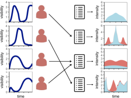
(b) Greedy algorithm

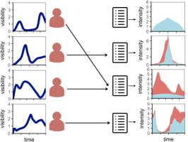
(c) CP baseline

Figure 3: Toy example with four broadcasters with budget $c_{i}=1$, four feeds, and $K=10$. Panel (a) shows the broadcasters’ intensities $\mu_{i}(t)$ and the feeds’ intensities due to other broadcasters $\gamma_{j\,|\,\mathcal{E}}$. Panels (b) and (c) show the solutions provided by the greedy algorithm and the CP baseline, respectively. In both panels, the left column shows the visibility $\mathcal{U}(i,j)$ and the right column shows the feed’s intensities due to the broadcasters and the other broadcasters.

C.4 Robustness of the greedy algorithm

To solve the visibility optimization problem defined in Eq. C.1 with Algorithm 1, we need to compute the average visibility, given by Eq. (33), which depends of a set of unknown intensities of the broadcasters and feeds. In practice, one could adopt a specific functional form for these intensities and fit them using historical data, however, that could lead to poor estimates of the visibility and, more importantly, it would be difficult to assess the impact of these empirical estimates on the approximation guarantees of the greedy algorithm. Instead, we can directly estimate the average visibility using historical data, derive a bound for the estimation error and assess how this estimation error impacts the approximation guarantees of the greedy algorithm.

Empirical estimation of the visibility. Given a directed network $\mathcal{G}=(\mathcal{V},\mathcal{E})$, a set of candidate links $\mathcal{E}_{\mathcal{B}}$, with $\tilde{\mathcal{E}}_{\mathcal{B}}\cap\mathcal{E}=\emptyset$, the intensities $\{\mu_{i}(t)\}_{i\in\mathcal{B}}$ of a set of broadcasters $\mathcal{B}\subseteq\mathcal{V}$, the users’ feed intensities $\{\gamma_{i\,|\,\mathcal{E}}(t)\}_{i\in\mathcal{V}}$ due to the broadcasters induced by the links $\mathcal{E}$, and $n$ sequences of posts of length $\Delta=t_{f}-t_{0}$, our empirical estimate of the average visibility $\mathcal{U}(\mathcal{E}_{\mathcal{B}},j)$ of the broadcasters in user $j$’s feed is given by

$$\hat{\mathcal{U}}(\mathcal{E}_{\mathcal{B}})=\sum_{j\in\mathcal{V}}\hat{\mathcal{U}}(\mathcal{E}_{\mathcal{B}},j)=\sum_{j\in\mathcal{V}}\frac{\sum_{i=1}^{K}\sum_{\ell=1}^{n}\Delta^{(\ell)}_{i,j}}{n},$$ (57)

where $\Delta^{(\ell)}_{i,j}$ is the amount of time that a post from the set of broadcasters $\mathcal{B}$ is at the $i$-th position of user $j$’s feed in realization $\ell$. Here, note that the empirical estimate does not explicitly depend on the intensities of the broadcasters and feeds and, given an arbitrary set of candidate links $\mathcal{E}_{\mathcal{B}}$, one can always measure the visibility they would reach without actual interventions.

We performed a formal analysis of the sample complexity of the above empirical estimate, however, for space constraints, we defer the details of this formal analysis to a longer version of the paper and here just state the main results. Let $0\leq y\leq 1$, we can show that:

$$\mathbb{P}\{\mathcal{U}(\mathcal{E}_{\mathcal{B}},j)-yK(t_{f}-t_{0})\leq\hat{\mathcal{U}}(\mathcal{E}_{\mathcal{B}},j)\leq\mathcal{U}(\mathcal{E}_{\mathcal{B}},j)+yK(t_{f}-t_{0})\}\geq 1-e^{Z_{y}-Q_{y}n},$$ (58)

where $Z_{y}$ and $Q_{y}$ are functions of, e.g.,

$$\beta_{j}=\inf_{t\in(t_{0},t_{f})}\frac{\mu(t)}{\mu(t)+\gamma_{j\,|\,\mathcal{E}}(t)},\,\,\rho_{j}=\sup_{t\in(t_{0},t_{f})}\frac{\mu(t)}{\mu(t)+\gamma_{j\,|\,\mathcal{E}}(t)},\,\,\mbox{and}\,\,\alpha.$$

Moreover, given the above error bound, we can characterize the approximation factor that the greedy algorithm achieves if it uses these empirical estimates:

Theorem 27.

Let the number of realizations $n\geq\frac{Z_{y}+\log\frac{\sum_{i\in\mathcal{B}}|\mathcal{W}_{i,:}|}{\delta}}{Q_{y}}$. Then, with probability at least $1-\delta$, the greedy algorithm returns a set of links $\mathcal{E}_{\mathcal{B}}$ such that

$$F(\mathcal{E}_{\mathcal{B}})\geq\frac{1}{\frac{1}{\xi}+1}OPT-4yK(t_{f}-t_{0})\sum_{i\in\mathcal{B}}c_{i},$$

where $OPT$ is the optimal value.

C.5 Experiments on synthetic data

Experimental setup. Unless stated otherwise, we use (periodic) piece-constant intensities $\mu_{i}(t)=\sum_{k=0}^{T-1}\mu_{i,k}\mathcal{I}(t\in[t_{k},t_{k+1}])$ and $\gamma_{j\,|\,\mathcal{E}}(t)=\sum_{j=0}^{T-1}\gamma_{j,k}\mathcal{I}(t\in[t_{k},t_{k+1}])$ for the broadcasters and the feeds, respectively, where $T=24$ days is the period, $t_{k+1}-t_{k}=1$ day is the length of each piece and, each piece, we pick $\mu_{i,k}$ and $\gamma_{j,k}$ uniformly at random. Note that, for piece-constant intensities, we are able to compute $\mathcal{U}(\mathcal{E}_{\mathcal{B}},j)$ analytically. We compare the performance of the greedy algorithm with the three heuristics from Section 5.2. Here, we will run both our greedy algorithm and the baselines using the true intensity values and then report the average (theoretical) value of visibility, however, note that all can be run using empirical estimates of the relevant quantities, i.e., $\mathcal{U}$ using Eq. 57 or $\int_{0}^{T}\gamma(t)dt$ using maximum likelihood estimation.

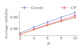
(a) $F(\mathcal{E}_{\mathcal{B}})$ vs. $K$

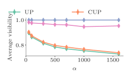
(b) $F(\mathcal{E}_{\mathcal{B}})$ vs. $\alpha$

Figure 4: Average visibility achieved by the greedy algorithm (GP) and the three heuristics (CP, UP, CUP) for a setting with $60$ broadcasters and $600$ feeds. Panel (a) shows the average visibility, $F(\mathcal{E}_{\mathcal{B}})$, for different $K$ values, where we sampled $\mu_{i,k}$ and $\gamma_{j,k}$ from $U[0.01,0.1]$ and $U[0.4,50]$, respectively, and $c_{i}=20$. Panel (b) shows the average visibility, normalized with respect to the visibility achieved by the greedy algorithm, where we sampled $\mu_{i,k}$ and $\gamma_{j,k}$ from $U[0.01,0.1]$ and $U[0.05,0.05]\times\alpha$, respectively, $K=10$ and $c_{i}=50$.

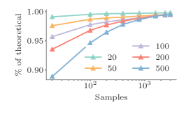
(a) $F(\mathcal{E}_{\hat{\mathcal{B}}})/F(\mathcal{E}_{\mathcal{B}})$ vs. $n$

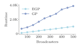
(b) Running time vs. # broadcasters

Figure 5: Robustness and running time of the greedy algorithm. Panel (a) compares the average visibility achieved by the solution $\mathcal{E}_{\mathcal{B}}$ ($\mathcal{E}_{\hat{\mathcal{B}}}$) provided by the greedy algorithm using the theoretical (empirical) visibility, where we sampled $\mu_{i,k}$ and $\gamma_{j,k}$ from $U[0.001,0.1]$ and $U[0.05,0.05\times\alpha]$, respectively, $K=10$ and $c_{i}=30$. Panel (b) shows the overall running time of the greedy algorithm using the theoretical (GP) and empirical (EGP) visibility, where we sampled $\mu_{i,k}$ and $\gamma_{j,k}$ from $U[0.001,0.1]$ and $U[0.05,0.05\times\alpha]$, $K=10$, and $c_{i}=30$.

Results. First, we experiment with a toy example with four broadcasters, each with budget $c_{i}=1$, and four feeds. Our goal here is to shed light on the way our greedy algorithm picks edges in comparison with one of the baselines. As illustrated in Figure 3, while the greedy algorithm identifies the times when each feed’s intensity due to other broadcasters is low and then picks a broadcaster for each feed whose intensity is high in those times, the baseline (CP) fails to recognize such optimal matchings.

Second, we compare the performance of the greedy algorithm and all baselines in a setting with $60$ broadcasters and $600$ feeds. Figure 4 summarizes the results, which show that the greedy algorithm beats the baselines by large margins under different $K$ and $\alpha$ values. We did experiment with a wide range of parameter settings (e.g., $K$, $\alpha$, $T$ or $c_{i}$) and found that the greedy algorithm consistently beats the baselines.

Third, we compare the visibility values achieved by the solution $\mathcal{E}_{\mathcal{B}}$ the greedy algorithm provides using the theoretical visibility, given by Eq. 37, against the solution $\mathcal{E}_{\hat{\mathcal{B}}}$ it provides using the empirical visibility, given by Eq. 57. Figure 5a summarizes the results, which show that, in agreement with Theorem 27, the quality of the solution the greedy algorithm provides using the empirical visibility converges to the one it provides using the theoretical visibility.

Finally, we compute the running time of the greedy algorithm against the number of broadcasters. Figure 5b summarizes the results, which show that the running time is linear in the number of walls. In additional experiments, we also found that the running time is linear in the number of walls, superlinear with respect to the number of pieces $T$ and it is independent on the budget per broadcaster, however, for space constraints, we do not include the corresponding plots.

References

• Altschuler et al. [2016] Jason Altschuler, Aditya Bhaskara, Gang Fu, Vahab Mirrokni, Afshin Rostamizadeh, and Morteza Zadimoghaddam. Greedy column subset selection: New bounds and distributed algorithms. In Proceedings of the 33rd International Conference on Machine Learning, 2016.
• Backstrom et al. [2011] L. Backstrom, E. Bakshy, J. M. Kleinberg, T. M. Lento, and I. Rosenn. Center of attention: How facebook users allocate attention across friends. In ICWSM, 2011.
• Bian et al. [2017] Andrew An Bian, Joachim M Buhmann, Andreas Krause, and Sebastian Tschiatschek. Guarantees for greedy maximization of non-submodular functions with applications. In Proceedings of the 34th International Conference on Machine Learning-Volume 70, pages 498–507. JMLR. org, 2017.
• Biega et al. [2018] Asia J Biega, Krishna P Gummadi, and Gerhard Weikum. Equity of attention: Amortizing individual fairness in rankings. In SIGIR, 2018.
• Bogunovic et al. [2018] Ilija Bogunovic, Junyao Zhao, and Volkan Cevher. Robust maximization of non-submodular objectives. 2018.
• Borodin et al. [2014] Allan Borodin, Dai Tri Man Le, and Yuli Ye. Weakly submodular functions. arXiv preprint arXiv:1401.6697, 2014.
• Calinescu et al. [2011] Gruia Calinescu, Chandra Chekuri, Martin Pál, and Jan Vondrák. Maximizing a monotone submodular function subject to a matroid constraint. SIAM Journal on Computing, 40(6):1740–1766, 2011.
• Candes et al. [2006] Emmanuel J Candes, Justin K Romberg, and Terence Tao. Stable signal recovery from incomplete and inaccurate measurements. Communications on Pure and Applied Mathematics: A Journal Issued by the Courant Institute of Mathematical Sciences, 59(8):1207–1223, 2006.
• Cha et al. [2010] M. Cha, H. Haddadi, F. Benevenuto, and K. Gummadi. Measuring user influence in twitter: The million follower fallacy. In ICWSM, 2010.
• Chen et al. [2018] Lin Chen, Moran Feldman, and Amin Karbasi. Weakly submodular maximization beyond cardinality constraints: Does randomization help greedy? In ICML, 2018.
• Conforti and Cornuéjols [1984] Michele Conforti and Gérard Cornuéjols. Submodular set functions, matroids and the greedy algorithm: tight worst-case bounds and some generalizations of the rado-edmonds theorem. Discrete applied mathematics, 7(3):251–274, 1984.
• Crawford [2015] M. Crawford. The world beyond your head: On becoming an individual in an age of distraction. Farrar, Straus and Giroux, 2015.
• Das and Kempe [2011] Abhimanyu Das and David Kempe. Submodular meets spectral: Greedy algorithms for subset selection, sparse approximation and dictionary selection. In Proceedings of the 28th International Conference on Machine Learning, 2011.
• De et al. [2019] Abir De, Utkarsh Upadhyay, and Manuel Gomez-Rodriguez. Temporal point processes. Technical report, Saarland University, 2019.
• Diamond and Boyd [2016] Steven Diamond and Stephen Boyd. Cvxpy: A python-embedded modeling language for convex optimization. The Journal of Machine Learning Research, 17(1):2909–2913, 2016.
• Du et al. [2008] Ding-Zhu Du, Ronald L Graham, Panos M Pardalos, Peng-Jun Wan, Weili Wu, and Wenbo Zhao. Analysis of greedy approximations with nonsubmodular potential functions. In Proceedings of the nineteenth annual ACM-SIAM symposium on Discrete algorithms, pages 167–175. Society for Industrial and Applied Mathematics, 2008.
• Elenberg et al. [2016] Ethan R Elenberg, Rajiv Khanna, Alexandros G Dimakis, and Sahand Negahban. Restricted strong convexity implies weak submodularity. arXiv preprint arXiv:1612.00804, 2016.
• Feige [2009] Uriel Feige. On maximizing welfare when utility functions are subadditive. SIAM Journal on Computing, 39(1):122–142, 2009.
• Feige and Vondrak [2006] Uriel Feige and Jan Vondrak. Approximation algorithms for allocation problems: Improving the factor of 1-1/e. In 2006 47th Annual IEEE Symposium on Foundations of Computer Science (FOCS’06), pages 667–676. IEEE, 2006.
• Filmus and Ward [2012] Yuval Filmus and Justin Ward. A tight combinatorial algorithm for submodular maximization subject to a matroid constraint. In 2012 IEEE 53rd Annual Symposium on Foundations of Computer Science, pages 659–668. IEEE, 2012.
• Fisher et al. [1978] Marshall L Fisher, George L Nemhauser, and Laurence A Wolsey. An analysis of approximations for maximizing submodular set functions—ii. In Polyhedral combinatorics, pages 73–87. Springer, 1978.
• Friedman [2004] Nir Friedman. Inferring cellular networks using probabilistic graphical models. Science, 303(5659):799–805, 2004.
• Friedman et al. [2000] Nir Friedman, Michal Linial, Iftach Nachman, and Dana Pe’er. Using bayesian networks to analyze expression data. Journal of computational biology, 7(3-4):601–620, 2000.
• Fujishige [2005] Satoru Fujishige. Submodular functions and optimization, volume 58. Elsevier, 2005.
• Gomez-Rodriguez et al. [2014] M. Gomez-Rodriguez, K. P. Gummadi, and B. Schoelkopf. Quantifying information overload in social media and its impact on social contagions. In ICWSM, 2014.
• Halabi et al. [2018] Marwa El Halabi, Francis Bach, and Volkan Cevher. Combinatorial penalties: Which structures are preserved by convex relaxations? 2018.
• Harshaw et al. [2019] Christopher Harshaw, Moran Feldman, Justin Ward, and Amin Karbasi. Submodular maximization beyond non-negativity: Guarantees, fast algorithms, and applications. In ICML, 2019.
• Hassani et al. [2017] Hamed Hassani, Mahdi Soltanolkotabi, and Amin Karbasi. Gradient methods for submodular maximization. In NIPS, 2017.
• Hodas and Lerman [2012] N. Hodas and K. Lerman. How visibility and divided attention constrain social contagion. In SocialCom, 2012.
• Horel and Singer [2016] Thibaut Horel and Yaron Singer. Maximization of approximately submodular functions. In Advances in Neural Information Processing Systems, pages 3045–3053, 2016.
• Irrthum et al. [2010] Alexandre Irrthum, Louis Wehenkel, Pierre Geurts, et al. Inferring regulatory networks from expression data using tree-based methods. PloS one, 5(9):e12776, 2010.
• Iyer and Bilmes [2012] Rishabh Iyer and Jeff Bilmes. Algorithms for approximate minimization of the difference between submodular functions, with applications. arXiv preprint arXiv:1207.0560, 2012.
• Kang and Lerman [2015] J. Kang and K. Lerman. Vip: Incorporating human cognitive biases in a probabilistic model of retweeting. In ICSC, 2015.
• Karimi et al. [2016] M. Karimi, E. Tavakoli, M. Farajtabar, L. Song, and M. Gomez-Rodriguez. Smart broadcasting: Do you want to be seen? In KDD, 2016.
• Krause and Guestrin [2005] Andreas Krause and Carlos E Guestrin. Near-optimal nonmyopic value of information in graphical models. In UAI, 2005.
• Krause et al. [2008] Andreas Krause, Ajit Singh, and Carlos Guestrin. Near-optimal sensor placements in gaussian processes: Theory, efficient algorithms and empirical studies. Journal of Machine Learning Research, 9(Feb):235–284, 2008.
• Lehmann et al. [2006] Benny Lehmann, Daniel Lehmann, and Noam Nisan. Combinatorial auctions with decreasing marginal utilities. Games and Economic Behavior, 55(2):270–296, 2006.
• Lerman and Hogg [2014] K. Lerman and T. Hogg. Leveraging position bias to improve peer recommendation. PloS one, 9(6):e98914, 2014.
• Lü and Zhou [2011] L. Lü and T. Zhou. Link prediction in complex networks: A survey. Physica A: statistical mechanics and its applications, 2011.
• Mirrokni et al. [2008] Vahab Mirrokni, Michael Schapira, and Jan Vondrák. Tight information-theoretic lower bounds for welfare maximization in combinatorial auctions. In Proceedings of the 9th ACM conference on Electronic commerce, pages 70–77. ACM, 2008.
• Narasimhan and Bilmes [2012] Mukund Narasimhan and Jeff A Bilmes. A submodular-supermodular procedure with applications to discriminative structure learning. arXiv preprint arXiv:1207.1404, 2012.
• Nemhauser et al. [1978] George L Nemhauser, Laurence A Wolsey, and Marshall L Fisher. An analysis of approximations for maximizing submodular set functions—i. Mathematical programming, 14(1):265–294, 1978.
• Powers et al. [2015] Thomas Powers, David W Krout, and Les Atlas. Sensor selection from independence graphs using submodularity. In 2015 18th International Conference on Information Fusion (Fusion), pages 333–337. IEEE, 2015.
• Schrijver [2003] Alexander Schrijver. Combinatorial optimization: polyhedra and efficiency, volume 24. Springer Science & Business Media, 2003.
• Singh and Joachims [2018] Ashudeep Singh and Thorsten Joachims. Fairness of exposure in rankings. In Proceedings of the 24th ACM SIGKDD International Conference on Knowledge Discovery & Data Mining, pages 2219–2228. ACM, 2018.
• Spasojevic et al. [2015] N. Spasojevic, Z. Li, A. Rao, and P. Bhattacharyya. When-to-post on social networks. In KDD, 2015.
• Tan et al. [2010] Vincent YF Tan, Animashree Anandkumar, and Alan S Willsky. Learning gaussian tree models: Analysis of error exponents and extremal structures. IEEE Transactions on Signal Processing, 58(5):2701–2714, 2010.
• Upadhyay et al. [2018] U. Upadhyay, A. De, and M. Gomez-Rodriguez. Deep reinforcement learning of marked temporal point processes. In NeurIPS, 2018.
• Vondrák [2008] Jan Vondrák. Optimal approximation for the submodular welfare problem in the value oracle model. In Proceedings of the fortieth annual ACM symposium on Theory of computing, pages 67–74. ACM, 2008.
• Vondrák [2010] Jan Vondrák. Submodularity and curvature: The optimal algorithm. 2010.
• Zarezade et al. [2017] A. Zarezade, U. Upadhyay, H. Rabiee, and M. Gomez-Rodriguez. Redqueen: An online algorithm for smart broadcasting in social networks. In WSDM, 2017.
• Zarezade et al. [2018] A. Zarezade, A. De, U. Upadhyay, H. Rabiee, and M. Gomez-Rodriguez. Steering social activity: A stochastic optimal control point of view. JMLR, 2018.