A Bivariate Spline Solution to the Exterior Helmholtz Equation
and its Applications

Abstract

We explain how to use smooth bivariate splines of arbitrary degree to solve the exterior Helmholtz equation based on a Perfectly Matched Layer (PML) technique. In a previous study (cf. [26]), it was shown that bivariate spline functions of high degree can approximate the solution of the bounded domain Helmholtz equation with an impedance boundary condition for large wave numbers $k\sim 1000$. In this paper, we extend this study to the case of the Helmholtz equation in an unbounded domain. The PML is constructed using a complex stretching of the coordinates in a rectangular domain, resulting in a weighted Helmholtz equation with Dirichlet boundary conditions. The PML weights are also approximated by using spline functions. The computational algorithm developed in [26] is used to approximate the solution of the resulting weighted Helmholtz equation. Numerical results show that the PML formulation for the unbounded domain Helmholtz equation using bivariate splines is very effective over a range of examples.

1 Introduction

We are interested in approximating the numerical solution of the Helmholtz equation over an exterior domain with the Sommerfeld radiation condition at infinity. The problem can be described as follows: Find the scattered field $u$ that satisfies

$$-\Delta u-k^{2}u=f\;\;\mbox{in}\;\;\mathbb{R}^{2}\setminus\overline{D},$$

$$u=g\;\;\mbox{on}\;\;\Gamma:=\partial D,$$

$$\lim_{r\rightarrow\infty}\sqrt{r}\left(\dfrac{\partial u}{\partial r}-iku\right)=0,\;\;r=|{\bf x}|,\;{\bf x}\in\mathbb{R}^{2}$$ (1)

where $D$ is a polygonal domain, $f$ is an $L^{2}$ integrable function with compact support over $\mathbb{R}^{2}\setminus\overline{D}$, $u$ is the solution to be solved and $k:=\omega/c$ is the wave number, $\omega$ being the angular frequency of the waves and $c$ the sound speed or speed of light dependent on the applications. The last equation, the Sommerfeld radiation condition, is assumed to hold uniformly in all directions. We assume that the wavenumber $k>0$ is constant. The more general case of inhomogeneous and anisotropic media will be considered in a future publication. In this paper, we assume a Dirichlet boundary condition on $D$, but the analysis and numerical results can be extended easily to Neumann or Robin boundary conditions.

The Helmholtz equation arises in many applications as a simplified model of wave propagation in the frequency domain. The modeling of acoustic and electromagnetic wave propagation in the time-harmonic regime are well-known examples. In particular, there is increasing interest in understanding electromagnetic scattering by subwavelength apertures or holes [34, 35, 36]. Scattering problems that involve periodic and layered media have also attracted attention [38, 20]. As a result, robust and accurate numerical algorithms for solving the Helmholtz equation have been studied over the years. For low frequencies, these problems can be handled using low order finite elements and finite differences. However as the wavenumber is increased, low order finite elements and finite differences become very expensive due to small mesh sizes that are needed to adequately resolve the wave. High order finite elements, least squares finite elements, Trefftz Discontinuous Galerkin methods have been proposed to handle large wavenumbers. In the case of wave propagation in unbounded domains, accurate treatment of truncation boundaries is also of paramount importance.

We plan to use bivariate spline functions to numerically solve the exterior Helmholtz problem [1]. Since our method involves a volumetric discretization, we need to truncate the unbounded domain while minimizing reflections from the artificial boundary. In an ideal framework, this truncation should satisfy at least three properties: efficiency, easiness of implementation, and robustness. There are several approaches available in the literature: infinite element methods (IFM)[40], boundary element methods (BEM) [8, 19], Dirichlet-to-Neumann operators (DtN) [15, 37, 21], Absorbing Boundary Conditions (ABC) [41], and Perfectly Matched Layer (PML) methods (e.g. [3] and many current studies). The BEM approach involves a discretization of the partial differential equation on a lower dimensional surface. In the DtN and ABC approaches, a Robin boundary condition is placed on the truncating boundary to absorb waves from the interior computational domain and to minimize reflections back into the domain. In PML approaches, a boundary layer of finite thickness is placed on the exterior of the computational domain to absorb and attenuate any waves coming from the interior. Moreover, the PML layer should preserve the solution inside the computational region of interest while exponentially damping the wave inside the PML region. Since the wave becomes exponentially small inside the PML layer, a hard Dirichlet boundary condition can be imposed on the exterior boundary of the PML layer.

The PML technique was first introduced in [Berenger, 1994[3]] in the context of Maxwell’s equations, but has now become an efficient approach for dealing with exterior domain wave propagation problems such as Helmholtz equations and Navier equations in two and three dimensions. Many PML functions have been designed and implemented. The original PML by Berenger was constructed in Cartesian coordinates for the Maxwell equations, and extended to curvilinear coordinates by Collino and Monk [12]. In [11], Chew and Wheedon demonstrated that the PML can be constructed by a complex change of variables.

In this paper, we shall use the PML technique in [23] and apply spline functions to solve (1). Bivariate and trivariate splines can be used for numerical solution of partial differential equations. We refer the reader to [2], [29], [22], [18], [28], [26], and etc.. In particular, in [26], the Helmholtz equation over a bounded domain in $\mathbb{R}^{2}$ is solved numerically by using bivariate spline functions. The researchers in [26] designed a bivariate spline method which very effectively solves the Helmholtz equation with large wave number with $k\geq 1000$. This paper is a complement of [26].

The rest of this paper is presented as follows. We first describe the PML formulation as a complex stretching of coordinates leading to a weighted Helmholtz equation. The exterior domain Helmholtz equation is then approximated by the PML problem with Dirichlet boundary conditions in a bounded domain. We apply the theory in [26] to show the well-posedness of the truncated PML problem. We next present bivariate splines and prove error estimates of the approximation of splines to the solution of the truncated PML problem. We finish with several numerical results that demonstrate the convergence of spline functions to the PML problem.

2 The PML formulation

We shall use a Cartesian PML for the scattering problem in the unbounded exterior of a 2D domain. We give a brief description of the setup, which can also be found in [23]. We shall assume $\Omega\subset\mathbb{R}^{2}$ is a bounded polygonal domain contained inside a rectangle $[-a_{1},a_{1}]\times[-a_{2},a_{2}]$ for some $a_{1},a_{2}>0$. The Cartesian PML is formulated in terms of the symmetric functions $\gamma_{1}(x_{1})$ and $\gamma_{2}(x_{2})$ for each point ${\bf x}=(x_{1},x_{2})$ in $\mathbb{R}^{2}\backslash\overline{\Omega}$. For some $b_{j}>0$ such that $0<a_{j}<b_{j}$, $j=1,2$ define the $\gamma_{j}$ by

$$\gamma_{j}(x_{j})=1+i\sigma_{j}(x_{j})$$

where the imaginary parts $\sigma_{j}$ are given by

$$\sigma_{j}(x_{j})=\left\{\begin{array}[]{@{}l@{\quad}l}0&\mbox{if $|x_{j}|<a_{j}$,}\\[3.0pt] \sigma_{0}\left(\dfrac{|x_{j}|-a_{j}}{b_{j}-a_{j}}\right)^{n}&\mbox{if $a_{j}\leq|x_{j}|\leq b_{j}$,}\\[3.0pt] \sigma_{0}&\mbox{if $|x_{j}|>b_{j}.$}\end{array}\right.$$

where $n$ is a non-negative integer usually $n=0,1,2,3,4$ in applications. Other PML functions can be considered, e.g. unbounded functions [5, 6]. In this paper we will consider only polynomial $\gamma_{j}$ defined above. We shall use the following notation $A=\mbox{diag}\left(\dfrac{\gamma_{2}(x_{2})}{\gamma_{1}(x_{1})},\dfrac{\gamma_{1}(x_{1})}{\gamma_{2}(x_{2})}\right)$ and $J=\gamma_{1}(x_{1})\gamma_{2}(x_{2})$. We denote by $\Omega_{\!{}_{F}}=([-a_{1},a_{1}]\times[-a_{2},a_{2}])\backslash\overline{D}$ the region outside the scatterer, and by $\Omega_{\!{}_{PML}}$ the PML region. We refer to Figure 1 for an illustration of the geometric setting.

Figure 1: An Illustration of the problem domain with a perfectly matched layer $\Omega_{\!{}_{PML}}$. The computational region of interest is the annulus $\Omega_{\!{}_{F}}$.

Then the exterior Helmholtz problem (1) is approximated by the truncated PML problem in $\Omega:=\Omega_{\!{}_{PML}}\cup\Omega_{\!{}_{F}}$: Find $u_{\rm PML}\in H^{1}_{\Gamma}(\Omega):=\{v\in H^{1}(\Omega):\;v=g\;\mbox{on}\;\Gamma,\;v=0,\;\mbox{on}\;\Gamma_{\!{}_{PML}}\}$

$$-\nabla\cdot A\nabla u_{\rm PML}-k^{2}Ju_{\rm PML} = f\;\;\hbox{ in }\Omega$$

$$u_{\rm PML} = g\;\;\hbox{ on }\;\;\Gamma$$

$$u_{\rm PML} = 0,\;\;\hbox{ on }\Gamma_{\!{}_{PML}}.$$ (2)

Note that inside $\Omega_{\!{}_{F}}$ we have $A=I$ and $J=1$ and the PML equation reduces to the standard Helmholtz equation. It is known that the truncated Cartesian PML problem above converges exponentially to the solution of the exterior Helmholtz equation inside the domain $\Omega_{\!{}_{F}}$ with a rate of convergence depending on the thickness of the PML layer and on the size of the parameter $\sigma_{0}$. Therefore it is sufficient to approximate the PML solution $u_{\rm PML}$ using bivariate splines. As the bivariate splines can efficiently and effectively solve the boundary value problem of Helmholtz equation as demonstrated in [26], we apply the bivariate splines to approximate the PML solution.

3 The Well-Posedness of the exterior domain Helmholtz equation

In this section we first present the existence, uniqueness and stability of the truncated Cartesian PML problem. Then we explain the approximation of the PML solution $u_{\rm PML}$ to the exact solution $u$ of (1).

Let $\mathbb{L}^{2}(\Omega)$ be the space of all complex-valued square integrable functions over $\Omega$ and $\mathbb{H}^{1}(\Omega)\subset\mathbb{L}^{2}(\Omega)$ be the complex-valued square integrable functions over $\Omega$ such that their gradients are in $\mathbb{L}^{2}(\Omega)$. Let $\mathbb{H}^{1}_{0}(\Omega)$ be the space of complex valued functions with bounded gradients which vanish on the boundary of $\Omega$. The weak formulation of the PML exterior domain Helmholtz equation can be defined in a standard fashion as follows. Find $u_{\rm PML}\in\mathbb{H}^{1}_{0}(\Omega)$ that satisfies $u_{\rm PML}|_{\Gamma}=g$, $u_{\rm PML}|_{\Gamma_{{\rm PML}}}=0$ and

$$\int_{\Omega}\left(A\nabla u_{\rm PML}\cdot\nabla\overline{v}-k^{2}Ju_{\rm PML}\overline{v}\right)\;d{\bf x} = \int_{\Omega}f\overline{v}\;d{\bf x}$$ (3)

for all $v\in\mathbb{H}^{1}_{0}(\Omega)$. For convenience, let $B_{k^{2}}(u_{\rm PML},v)$ be the sesquilinear form on the left hand side of (3). The above equation can then be simply rewritten as

$$B_{k^{2}}(u_{\rm PML},v)=\langle f,v\rangle_{\Omega},\quad\forall v\in\mathbb{H}^{1}_{0}(\Omega).$$ (4)

where $\langle f,v\rangle_{\Omega}=\int_{\Omega}f\overline{v}d{\bf x}$. We shall use the Fredholm alternative theorem to establish the existence and uniqueness of the PML weak solution $u_{\rm PML}$.

Consider the following two second order elliptic partial differential equations:

$$\begin{cases}B_{\lambda}(u,v)&=0,\hbox{ in }\Omega\cr u&=0,\hbox{ in }\partial\Omega\end{cases}$$ (5)

and

$$\begin{cases}B_{\lambda}(u,v)&=\langle f,v\rangle_{\Omega},\hbox{ in }\Omega\cr u&=0,\hbox{ in }\partial\Omega,\end{cases}$$ (6)

where $\lambda>0$ is a constant, $f\in L^{2}(\Omega)$. We have the following well-known result:

Theorem 1 (Fredholm Alternative Theorem)

Fix $\lambda>0$. Precisely one of the following two statements holds: Either (5) has a nonzero weak solution $u\in\mathbb{H}^{1}(\Omega)$ or there exists a unique weak solution $u_{f}\in\mathbb{H}^{1}(\Omega)$ satisfying (6).

• Proof. We refer to [13] for a proof. $\Box$

Theorem 2

Let $g\in H^{-1/2}(\Gamma)$ and $f\in L^{2}(\Omega)$. Suppose that $\sigma_{j},j=1,2$ be bounded, continuous, non-negative and monotonically increasing functions. Then, the truncated PML problem (2) has a unique weak solution $u_{\rm PML}\in\mathbb{H}^{1}(\Omega)$ in the sense of (4) for every real value $k$, except at most for a discrete set of values of $k$.

• Proof. If $k^{2}$ is not an eigenvalue of (5), then we use Fredholm Alternative Theorem 1 to conclude that the PDE in (6) has a unique solution. Otherwise, it is well-known that there are only countable numbers of eigenvalues of the Dirichlet problem of Laplace operator and these eigenvalues $\lambda_{i}>0,i=1,2,\cdots,\infty$ with $\lambda_{j}\to\infty$. $\Box$

Next we discuss the stability of the weak solution $u_{\rm PML}$. To analyze the weak formulation, it is convenient to introduce the following norm which is equivalent to the standard $H^{1}$ norm:

$${|||}u{|||}_{H}^{2}= \int_{\Omega}\left(\sum_{j=1}^{2}|A_{jj}|\left|\dfrac{\partial u}{\partial x_{j}}\right|^{2}+k^{2}|J||u|^{2}\right)\;d{\bf x}$$ (7)

$$= |u|^{2}_{H}+k^{2}\|u\|^{2}_{H}$$ (8)

where $|u|^{2}_{H}=\int_{\Omega}\sum_{j=1}^{2}|A_{jj}|\left|\partial_{x_{j}}u\right|^{2}\;d{\bf x}$ the PML weighted $\mathbb{H}^{1}(\Omega)$ semi-norm and by $\|u\|^{2}_{H}=\int_{\Omega}|J||u|^{2}d{\bf x}$ the weighted $\mathbb{L}^{2}(\Omega)$ norm.

The following continuity condition of the sesquilinear form $B_{k^{2}}(u,v)$ can be obtained easily.

Lemma 1

Suppose that $f\in L^{2}(\Omega)$. Then

$$|B_{k^{2}}(u,v)|\leq C_{B}{|||}u{|||}_{H}\,{|||}v{|||}_{H},$$ (9)

where $C_{B}$ is a positive constant dependent on $\Omega$ only.

One of the major theoretical results in this paper is the following

Theorem 3

Let $\Omega\subset\mathbb{R}^{2}$ be a bounded Lipschitz domain. Suppose that $k^{2}$ is not a Dirichlet eigenvalue of (5) over $\Omega$. Then there exists $C_{*}>0$ which does not go to zero when $k\to\infty$ such that

$$\inf_{v\in\mathbb{H}^{1}(\Omega)}\sup_{u\in\mathbb{H}^{1}(\Omega)}\frac{\hbox{Re}(B_{k^{2}}(u,v))}{{|||}u{|||}_{H}\,{|||}v{|||}_{H}}\geq C_{*}.$$ (10)

• Proof. Suppose (10) does not hold. Then there exists $v_{n}\in\mathbb{H}^{1}(\Omega)$ such that ${|||}v_{n}{|||}_{H}=1$ and

  $$\sup_{u\in\mathbb{H}^{1}(\Omega)}\frac{\hbox{Re}(B_{k^{2}}(u,v_{n}))}{{|||}u{|||}_{H}}\leq\frac{1}{n}$$

  for $n=1,\cdots,\infty$. The boundedness of $v_{n}$ implies that there exists a convergent subsequence that converges in $\mathbb{L}^{2}(\Omega)$, by the Rellich-Kondrachov Theorem. Without loss of generality we may assume that $v_{n}\to v^{*}$ in the $\mathbb{L}^{2}(\Omega)$ norm and in the semi-norm on $\mathbb{H}^{1}(\Omega)$ with ${|||}v^{*}{|||}_{H}=1$. It follows that for each $u\in\mathbb{H}^{1}(\Omega)$ with ${|||}u{|||}_{H}=1$, $\hbox{Re}(B_{k^{2}}(u,v_{n}))\to 0$. Hence, $\hbox{Re}(B_{k^{2}}(u,v^{*}))=0$ for all $u\in\mathbb{H}^{1}(\Omega)$. By using $u=v^{*}$, we see that $B_{k^{2}}(v^{*},v^{*}))=0$.

  So if $v^{*}\not=0$, $v^{*}\in\mathbb{H}^{1}_{0}(\Omega)$ is an eigenfunction with eigenvalue $k^{2}$ of the Dirichlet problem for the truncated homogeneous PML problem (5). This contradicts the assumption that $k^{2}$ is not a Dirichlet eigenvalue of (5). Hence, we have $v^{*}\equiv 0$ which contradicts to the fact ${|||}v^{*}{|||}_{H}=1$. Therefore, $C_{*}>0$ in (10).

  We next show that $C_{*}$ does not go to zero when $k\to\infty$. For each integer $k>0$, let $L_{k}$ be the best lower bound in (10). We claim that $L_{k}\not\to 0$. Indeed, for $L_{k}>0$, we can find $v_{k}$ with ${|||}v_{k}{|||}_{H}=1$ such that

  $$\sup_{u\in\mathbb{H}^{1}(\Omega)}\frac{\hbox{Re}(B_{k^{2}}(u,v_{k}))}{{|||}u{|||}_{H}}\leq 2L_{k}.$$

  That is, $\hbox{Re}(B_{k^{2}}(v_{k},v_{k}))\leq 2L_{k}$. Since $|v_{k}|_{H}\leq 1$ and $k^{2}\|v_{k}\|_{H}^{2}\leq 1$ or $\|v_{k}\|_{H}\leq 1/k\leq 1$, we use Rellich-Kondrachov Theorem again to conclude that there exists a $u^{*}\in\mathbb{H}^{1}(\Omega)$ such that $v_{k}\to u^{*}$ in $L^{2}$ norm and $|v_{k}|_{H}\to|u^{*}|_{H}$ without loss of generality. As $\|v_{k}\|_{H}\leq 1/k$, we have $\|u^{*}\|_{H}\leq 2/k$ for $k>0$ large enough. It follows that $u^{*}\equiv 0$. Thus, $\nabla u^{*}\equiv 0$, that is, $|u^{*}|_{H}=0$. Hence, $|v_{k}|_{H}\to 0$. If $L_{k}\to 0$, we have $\large{|}|v_{k}|_{H}^{2}-k^{2}\|v_{k}\|_{H}^{2}\large{|}=|\hbox{Re}(B_{k^{2}}(v_{k},v_{k}))|\to 0$. It follows that $k^{2}\|v_{k}\|_{H}^{2}\to 0$. However, since ${|||}v_{k}{|||}_{H}=1$, we have $k^{2}\|v_{k}\|_{H}^{2}\to 1$. That is, we got a contradiction. Therefore, $L_{k}$ does not go to zero when $k\to\infty$. $\Box$

Furthermore, the weak solution is stable. Indeed,

Theorem 4

Let $\Omega\subset\mathbb{R}^{2}$ be a bounded Lipschitz domain as described in the introduction section. Suppose that $k^{2}$ is not a Dirichlet eigenvalue of the elliptic PDE (5) over $\Omega$. Let $u_{\rm PML}\in\mathbb{H}^{1}(\Omega)$ be the unique weak solution to (3) as in Theorem 2. Then there exists a constant $C>0$ independent of $f$ such that

$${|||}u_{\rm PML}{|||}_{H}\leq C\|f\|$$ (11)

for $k\geq 1$, where $C$ is dependent on the constant $C_{*}$ which is the lower bound in (10) and hence, $C$ will not go to $\infty$ as $k\to\infty$.

• Proof. Let $u_{\rm PML}$ be the weak solution of the exterior domain Helmholtz equation satisfying (1). By using (10), we have

  $$C_{*}{|||}u_{\rm PML}{|||}_{H} \leq\sup_{u\in\mathbb{H}^{1}(\Omega)}\frac{\hbox{Re}(B_{k^{2}}(u,u_{\rm PML}))}{{|||}u{|||}_{H}}=\sup_{u\in\mathbb{H}^{1}(\Omega)}\frac{\hbox{Re}(\langle u,f\rangle_{\Omega}}{{|||}u{|||}_{H}}\leq\|f\|$$ (12)

  by using Cauchy-Schwarz inequality in the last step. $\Box$

We refer to [7, 23] for more properties of the weak solution $u_{\rm PML}$. In particular it is known that $u_{\rm PML}$ approximates the solution $u$ of exterior domain Helmholtz equation (1) very well. Indeed, in [7], we saw if $\sigma_{0}$ is the PML strength, and $M=b-a$ is the size of the PML layer with stretching functions in the $x_{1}$ and $x_{2}$ directions equal, for convenience, then the truncated PML problem is stable provided that $M\sigma_{0}$ is sufficiently large. Moreover, the solution of the truncated PML problem 6 converges exponentially to the solution of the exterior Helmholtz problem 1. More precisely, the following result can be found in [7].

Theorem 5 (Theorem 5.8 of [7])

Suppose that $\sigma_{0}M$ is large enough. Let $g\in H^{1/2}(\Gamma)$ be given, $u$ be the solution of the exterior Helmholtz problem (1) with $f\equiv 0$ and $u_{{\rm PML}}$ be the solution of the truncated PML problem. Then there exist constants $c>0,C>0$ such that,

$$\|u-u_{\rm PML}\|_{H^{1}(\Omega)}\leq Ce^{-c\sigma_{0}M}\|g\|_{H^{1/2}(\Gamma)}.$$ (13)

The result of Theorem 5 justifies the use of the PML technique to truncate the exterior Helmholtz problem. Furthermore, Theorem 5 also shows that good accuracy can be achieved by simply increasing the value of the PML parameter $\sigma_{0}$ on a fixed grid. Numerical behavior of $\sigma$ vs. $M$ can be found in a later section.

4 Bivariate Spline Spaces and Spline Solutions

Let us begin by reviewing some basic properties of bivariate spline spaces which will be useful in the study in this paper. We refer to [27] and [2] for details. Given a polygonal region $\Omega:=\Omega_{\rm PML}$, a collection $\triangle:=\{T_{1},...,T_{n}\}$ of triangles is an ordinary triangulation of $\Omega$ if $\Omega=\cup_{i=1}^{n}T_{i}$ and if any two triangles $T_{i},T_{j}$ intersect at most at a common vertex or a common edge. We say $\triangle$ is $\beta$ quasi-uniform if

$$\max_{T\in\triangle}\frac{|T|}{\rho_{T}}\leq\beta<\infty$$ (14)

where $\rho_{T}$ is the radius of the inscribed circle of $T\in\triangle$. For $r\geq 0$ and $d>r$, let

$$S^{r}_{d}(\triangle)=\{s\in C^{r}(\Omega):s|_{T}\in\mathbb{P}_{d},\forall T\in\triangle\}$$ (15)

be the spline space of degree $d$ and smoothness $r\geq 0$ over triangulation $\triangle$.

Let us quickly explain the structure of spline functions in $S^{r}_{d}(\triangle)$. For a triangle $T_{i}\in\triangle$, $T_{i}=(v_{1},v_{2},v_{3})$, we define the barycentric coordinates $(b_{1},b_{2},b_{3})$ of a point $(x_{o},y_{o})\in\Omega$. These coordinates are the solution of the following system of equations

$$b_{1}+b_{2}+b_{3}=1$$

$$b_{1}v_{1,x}+b_{2}v_{2,x}+b_{3}v_{3,x}=x_{o}$$

$$b_{1}v_{1,y}+b_{2}v_{2,y}+b_{3}v_{3,y}=y_{o},$$

and are nonnegative if $(x_{o},y_{o})\in T_{i}$, where $v_{1,x}$ denotes the $x$ coordinate of vertex $v_{1}$. The barycentric coordinates are then used to define the Bernstein polynomials of degree $d$:

$$B^{T}_{i,j,k}(x,y):=\frac{d!}{i!j!k!}b_{1}^{i}b_{2}^{j}b_{3}^{k},\hskip 28.45274pti+j+k=d.$$

which form a basis for the space $\mathcal{P}_{d}$ of polynomials of degree $d$. Therefore we can represent all $P\in\mathcal{P}_{d}$ in B-form:

$$P=\sum_{i+j+k=d}p_{ijk}B^{T}_{ijk},$$

where the $B$-coefficients $p_{ijk}$ are uniquely determined by $P$.

We define the spline space $S^{-1}_{d}:=\{s|_{T_{i}}\in\mathcal{P}_{d}\},T_{i}\in\triangle$, where $T_{i}$ is a triangle in a triangulation $\triangle$ of $\Omega$. We use this piecewise continuous polynomial space to define

$$S^{r}_{d}:=C^{r}(\Omega)\cap S^{0}_{d}(\triangle),$$ (16)

See properties and implementation of these spline spaces in [27] and a method of implementation of multivariate splines in [2]. We include information about spline smoothness here which is significantly different from the finite element method and discontinuous Galerkin method. Note that the implementation of bivariate splines in [39] is similar to the finite element.

We start with the recurrence relation (de Castlejau algorithm)

$$B^{d}_{ijk}=b_{1}B^{d-l}_{i-1,j,k}+b_{2}B^{d-l}_{i,j-1,k}+b_{3}B^{d-l}_{i,j,k-1},\quad\textnormal{for all }i+j+k=d,$$

where all items with negative subscripts are taken to be 0, allows us to define ${\bf c}^{(0)}={\bf c}$ with

$${\bf c}^{(0)}_{ijk}:=p_{ijk},i+j+k=d.$$

Then for $\l=1,...,d$, we have ${\bf c}^{\l}$ with

$${\bf c}^{(\l)}_{ijk}=b_{1}{\bf c}^{(\l-1)}_{i+1,j,k}+b_{2}{\bf c}^{(\l-1)}_{i,j+1,k}+b_{3}{\bf c}^{(\l-1)}_{i,j,k+1},$$

so, letting $u=(x,y)$, we can write

$$P(u)=\sum_{i+j+k=d-\l}{\bf c}^{(\l)}_{ijk}B^{d-\l}_{ijk}(u).$$

Let $u,v\in\mathbb{R}^{2}$ be represented in barycentric coordinates by $(\alpha_{1},\alpha_{2},\alpha_{3})$ and $(\beta_{1},\beta_{2},\beta_{3})$ respectively. Then the vector $a=u-v$ is given in barycentric coordinates by $a_{i}=\alpha_{i}-\beta_{i}$, and the derivative in that direction is given by

$$a\cdot\nabla B_{ijk}^{d}(v)=d\big{(}a_{1}B^{d-l}_{i-1,j,k}+a_{2}B^{d-l}_{i,j-1,k}+a_{3}B^{d-l}_{i,j,k-1}\big{)}$$ (17)

for any $i+j+k=d$. With the above, we can derive smoothness conditions as follows.

Consider two triangles $T_{1}=(v_{1},v_{2},v_{3})$ and $T_{2}=(v_{4},v_{3},v_{2})$ joined along the edge $e_{23}=\langle v_{2},v_{3}\rangle$. Let

$$p(x,y):=\sum_{i+j+k=d}c_{ijk}B^{d}_{ijk}(x,y),\quad\quad q(x,y):=\sum_{i+j+k=d}r_{ijk}R^{d}_{ijk}(x,y)$$

To enforce continuity of the spline consisting of $p$ and $q$ over domain $T_{1}\cup T_{2}$, we enforce $p(x,y)|_{e_{23}}=q(x,y)|_{e_{23}}$ which leads to the condition $c_{0}jk=r_{0}kj$ for all $j+k=d$. This also guarantees that the derivatives in a direction tangent to $e_{23}$ will match. Next we take a direction ${\bf a}$ not parallel to $e_{23}$ whose barycentric coordinates with respect to $T_{1}$ and $T_{2}$ are denoted $\alpha$ and $\beta$, respectively. We require

$${\bf a}\cdot\nabla p(x,y)|_{e_{23}} ={\bf a}\cdot\nabla q(x,y)|_{e_{23}}$$

or

$$d\sum_{j+k=d-1}{\bf c}^{(1)}_{0jk}(\alpha)B_{0jk}^{d-1}(v) =d\sum_{j+k=d-1}{\bf r}^{(1)}_{0jk}(\beta)R_{0jk}^{d-1}(v),$$

where ${\bf c}$, ${\bf r}$ are iterates of the de Casteljau algorithm mentioned above.

But on $e_{23}$ we have $B_{0jk}=R_{0kj}$, so it follows that the derivatives of $p$ and $q$ will match on $e_{23}$ if and only if

$${\bf c}^{(1)}_{0jk}(\alpha)={\bf r}^{(1)}_{0kj}(\beta).$$

See more detail in [27] for higher order smoothness.

It is clear to see that the smoothness conditions are linear equations in terms of coefficient vector ${\bf c}=[c_{ijk},i+j+k=d]\cup[r_{ijk},i+j+k=d]$. The $C^{0}$ and $C^{1}$ smoothness conditions can be equivalently written as linear system $H{\bf c}=0$. In general, we collect the coefficients of all polynomials over triangles in $\triangle$ and put them together to form a vector ${\bf c}$ and put all smoothness conditions together to form a set of smoothness constraints $H{\bf c}=0$. Certainly, more detail can be found in [27]. We refer [2] for how to implement these spline functions for numerical solution of some basic partial differential equations. See [29], [22], [18], [28], [26] for spline solution to other PDEs.

As solutions to the Helmholtz equation will be a complex valued solution, let us use a complex spline space in this paper defined by

$$\mathbb{S}^{r}_{p}(\triangle)=\{s=s_{r}+{\bf i}s_{i},s_{i},s_{r}\in S^{r}_{p}(\triangle)\}.$$ (18)

The complex spline space $\mathbb{S}^{r}_{p}(\triangle)$ has the similar approximation properties as the standard real-valued spline space $S^{r}_{p}(\triangle)$. The following theorem can be established by the same constructional techniques (cf. [27] for spline space $S^{r}_{p}(\triangle)$ for real valued functions):

Theorem 6

Suppose that $\triangle$ is a $\gamma$-quasi-uniform triangulation of polygonal domain $\Omega$. Let $p\geq 3r+2$ be the degree of spline space $\mathbb{S}_{p}^{r}(\triangle)$. For every $u\in\mathbb{H}^{m+1}(\Omega)$, there exists a quasi-interpolatory spline function $Q_{p}(u)\in\mathbb{S}^{r}_{p}(\triangle)$ such that

$$\sum_{T\in\triangle}\|D^{\alpha}_{x}D^{\beta}_{y}(u-Q_{p}(u))\|^{2}_{2,T}\leq K_{5}|\triangle|^{2(m+1-s)}|u|^{2}_{2,p+1,\Omega}$$ (19)

for $\alpha+\beta=s,0\leq s\leq m+1$, where $0\leq m\leq p$, $K_{5}$ is a positive constant dependent only on $\gamma$, $\Omega$, and $p$.

With the above preparation, we now introduce spline weak solution to (1). Let $s_{\rm PML}\in\mathbb{S}^{r}_{p}(\triangle)$ be a spline function satisfying $s_{\triangle}|_{\Gamma}=g$ and the weak formulation:

$$B_{k^{2}}(s_{\triangle},v)=\langle f,v\rangle_{\Omega},\quad\forall v\in\mathbb{S}^{r}_{p}(\triangle)\cap\mathbb{H}^{1}_{0}(\Omega).$$ (20)

$s_{\rm PML}$ is called a PML solution of (1). We will show that $s_{\rm PML}$ approximates the PML solution $u_{\rm PML}$ discussed in the previous section.

To do so, we first explain the well-posedness of $s_{\rm PML}$. Similar to Theorem 2 and 3 in the previous section, we have

Theorem 7

Let $\Omega\subset\mathbb{R}^{2}$ be a bounded Lipschitz domain. Suppose that $k^{2}$ is not a Dirichlet eigenvalue of (5) over $\Omega$. Let $\mathbb{S}^{1}_{p}(\triangle)$ be the complex valued spline space defined above, where $\triangle$ is a triangulation of $\Omega$. Then there exists a unique spline weak solution $s_{\rm PML}\in\mathbb{S}^{1}_{p}(\triangle)$ satisfying (20). Furthermore, $s_{\rm PML}$ is stable in the sense that

$${|||}s_{\rm PML}{|||}_{H}\leq C\|f\|_{2,\Omega}.$$

where $C>0$ is a constant does not go to $\infty$ when $k\to\infty$.

Next we discuss the approximation of $s_{\rm PML}$ to the PML solution $u_{\rm PML}$. The orthogonality condition follows easily:

$$B_{k^{2}}(u_{\rm PML}-s_{\rm PML},v)=0,\quad\forall v\in\mathbb{S}^{r}_{p}(\triangle)\cap\mathbb{H}^{1}_{0}(\Omega).$$ (21)

For convenience, let us first consider homogeneous Helmholtz equation. That is, $f\equiv 0$ in (1). Thus we are ready to prove one of the following main results in this paper.

Theorem 8

Let $\Omega$ be a bounded Lipschitz domain as defined in the introduction. Suppose that $k^{2}$ is not a Dirichlet eigenvalue of the elliptic PDE in (5). Let $u_{\rm PML}$ be the unique weak solution in $\mathbb{H}^{1}(\Omega)$ satisfying (3) and $s_{\rm PML}\in\mathbb{S}^{r}_{p}(\triangle)$ be the spline weak solution satisfying (31). Suppose that the exact solution $u\in\mathbb{H}^{s}(\Omega)$ of (1) with $1\leq s\leq p$. Then there exists a positive constant $C>0$ which does not go to $\infty$ when $k\to\infty$ such that

$${|||}u-s_{\rm PML}{|||}_{H}\leq C\exp(-c\sigma_{0}M)\|g\|_{H^{1/2}(\Gamma)}+C(1+k|\triangle|)|\triangle|^{s-1}|u_{\rm PML}|_{s,2,\Omega},$$ (22)

where $|u_{\rm PML}|_{s,2,\Omega}$ is the semi-norm in $\mathbb{H}^{s}(\Omega)$.

• Proof. We first apply the lower bound in Theorem 2 to $u-s_{\rm PML}$ and have

  $$C_{*}{|||}u_{\rm PML}-s_{\rm PML}{|||}^{2}_{H}\leq|B_{k^{2}}(u_{\rm PML}-s_{\rm PML},u_{\rm PML}-s_{\rm PML})|.$$ (23)

  Next we use the orthogonality condition (21) to have

  $$|B_{k^{2}}(u_{\rm PML}-s_{\rm PML},u_{\rm PML}-s_{\rm PML})| = |B_{k^{2}}(u_{\rm PML}-s_{\rm PML},u_{\rm PML}-Q_{p}(u_{\rm PML})|$$

  $$\leq C_{B}{|||}u_{\rm PML}-s_{\rm PML}{|||}_{H}{|||}u_{\rm PML}-Q_{p}(u_{\rm PML}){|||}_{H}$$

  by using Lemma 1, i.e. (9), where $Q_{p}(u_{\rm PML})$ is the quasi-interpolatory spline of $u_{\rm PML}$ as in Theorem 6. It follows that

  $${|||}u_{\rm PML}-s_{\rm PML}{|||}_{H}\leq C_{*}^{-1}C_{B}{|||}u_{\rm PML}-Q_{p}(u_{\rm PML}){|||}_{H}.$$ (24)

  Finally, we use the approximation property of spline space $\mathbb{S}^{r}_{p}(\triangle)$, i.e. (19). For $u_{\rm PML}\in\mathbb{H}^{s}(\Omega)$ with $1\leq s\leq p$, we use the quasi-interpolatory operator $Q_{p}(u_{\rm PML})$ to have

  $${|||}u_{\rm PML}-Q_{p}(u_{\rm PML}){|||}_{H}\leq C(1+k|\triangle|)|\triangle|^{s-1}|u_{\rm PML}|_{s,2,\Omega}$$

  for a constant $C$ dependent on $\omega$, $p$ and the smallest angle of $\triangle$ only.

  Now we can use Theorem 5 to finish the proof. Indeed, we combine the estimates above with the estimate in 13 to have

  $${|||}u-s_{\rm PML}{|||}_{H} \leq {|||}u-u_{\rm PML}{|||}_{H}+{|||}u_{\rm PML}-s_{\rm PML}{|||}_{H}$$ (25)

  $$\leq C_{1}\exp(-cM\sigma_{0})\|g\|_{H^{1/2}(\Gamma)}+C_{2}(1+k|\triangle|)|\triangle|^{s-1}|u_{\rm PML}|_{s,2,\Omega},$$ (26)

  where $c>0,C_{1}$ are positive constants as in Theorem 5 and $C_{2}>0$ is another positive constant dependent on the lower bound $C_{*}$ and the approximation property in Theorem 6. $\Box$

Next let $u_{f,g}$ be the exact solution of (1) and let $u_{f,0}$ be the weak solution of

$$-\Delta u-k^{2}u=f\;\; \mbox{in}\;\;\mathbb{R}^{2}\setminus\overline{D}$$

$$u=0\;\; \mbox{on}\;\;\Gamma:=\partial D,$$

$$\lim_{r\rightarrow\infty}\sqrt{r}\left(\dfrac{\partial u}{\partial r}-iku\right)=0,\;\; r=|{\bf x}|,\;{\bf x}\in\mathbb{R}^{2}.$$

by using Theorem 1. We extend $u_{f,0}$ outside of $\Omega$ by zero naturally. We know $u=u_{f,g}-u_{f,0}$ satisfies the exterior domain problem (1) of Helmholtz equation with Sommerfeld radiation condition at $\infty$. Then by Theorem 5, there exists a PML solution $u_{PML}$ which converges to $u$ very well satisfying (13). Let $s_{f,0}$ be the spline approximation of the elliptic PDE (4). In fact, $s_{f,0}$ is the spline solution to the following boundary value problem:

$$-\Delta u-k^{2}u=f\;\; \mbox{in}\;\;\Omega,$$ (28)

$$u=0\;\; \mbox{on}\;\;\partial\Omega.$$

According to [2], we can find a spline approximation $s_{f,0}$ to the exact solution $u$ of the PDE above as long as $k^{2}$ is not an eigenvalue of Dirichlet problem of the Laplace operator over $\Omega$. By extending $s_{f,0}$ outside of $\Omega$ by zero, we see that $s_{f,0}$ is a good approximation of $u_{f,0}$ satisfying the Sommerfeld radiation condition in (4).

Let $u_{\rm PML}$ be the PML approximation of (1) and $s_{\rm PML}$ be the spline approximation of (1) with $f=0$. Let

$$s_{\triangle}=s_{f,0}+s_{\rm PML}$$ (29)

be the spline weak solution to the original PDE (1). Then we can show

$$\|u_{f,g}-s_{\triangle}\| = \|u_{f,g}-s_{f,0}-s_{\rm PML}\|=\|u_{f,g}-u_{f,0}-u_{\rm PML}+\|u_{f,0}-s_{f,0}+u_{\rm PML}-s_{\rm PML}\|$$

$$\leq \|u-u_{\rm PML}\|+\|u_{f,0}-s_{f,0}\|+\|u_{\rm PML}-s_{\rm PML}\|.$$

We use Theorem 5 to the first term, Theorem 8 in [2] to the middle term, and a part of the proof of Theorem 8 to the last term on the right-hand side of the above estimate.

Theorem 9

Let $\Omega$ be a bounded Lipschitz domain as defined in the introduction. Suppose that $k^{2}$ is not a Dirichlet eigenvalue of the elliptic PDE in (5), nor a Dirichlet eigenvalue of the Laplace operator over $\Omega$. Let $u_{\rm PML}$ be the unique weak solution in $\mathbb{H}^{1}(\Omega)$ satisfying (4) and $s_{\rm PML}\in\mathbb{S}^{r}_{p}(\triangle)$ be the spline weak solution satisfying (31). Suppose that the exact solution $u_{f,g}\in\mathbb{H}^{s}(\Omega)$ of (1) with $1\leq s\leq p$. Similarly, suppose that the exact solution $u_{f,0}\in\mathbb{H}^{s}(\Omega)$ of (4). Then there exists a positive constant $C>0$ which does not go to $\infty$ when $k\to\infty$ such that

$${|||}u_{f,g}-s_{\triangle}{|||}_{H}\leq C\exp(-c\sigma_{0}M)\|g\|_{H^{1/2}(\Gamma)}+C(1+k|\triangle|)|\triangle|^{s-1}|u_{f,0}|_{s,2,\Omega}+C(1+k|\triangle|)|\triangle|^{s-1}|u_{\rm PML}|_{s,2,\Omega},$$ (30)

where $|u_{\rm PML}|_{s,2,\Omega}$ is the semi-norm in $\mathbb{H}^{s}(\Omega)$.

5 Numerical Implementation

The implementation of bivariate splines is different from the traditional finite element method and the spline method in [39]. It builds a system of equations with smoothness constraints (across interior edges) and boundary condition constraints and then solves a constrained minimization instead of coding all smoothness and boundary condition constraints into basis functions and then solving a linear system of smaller size. The constrained minimization is solved using an iterative method with a very few iterations. See an explanation of the implementation in [2]. Several advantages of the implementation in [2] are:

• (1) piecewise polynomials of any degree $p\geq 1$ and higher order smoothness can be used easily. Certainly, they are subject to the memory of a computer. We usually use $p=5$ and often use $p=5,\cdots,15$ together with the uniform refinement or adaptive refinement to obtain the best possible solution within the budget of computer memory.

• (2) there is no quadrature formula. The computation of the related inner product and triple product is done using formula; Note that the right-hand side function $f$ is approximated by using a continuous spline if $f$ is continuous or a discontinuous spline function $s_{f}\in\mathbb{S}^{-1}_{p}(\triangle)$.

• (3) the computation of the mass matrix and weighted stiffness matrix is done in parallel;

• (4) the matrices for the smoothness conditions (across interior edges) and boundary conditions are done in parallel and are used as side constraints during the minimization of the discrete partial differential equations.

• (5) Using spline functions of higher degree than 1, the bivariate spline method can find accurate solution without using a pre-conditioner as shown in Example 4 in the next section.

In addition to triangulations, the implementation in [2] has been extended to the setting of polygonal splines of arbitrary degrees over a partition of polygons of any sides (cf. [14] and [25]).

Our computational algorithm is given as follows. For spline space $\mathbb{S}^{1}_{p}(\triangle)$, let ${\bf c}$ be the coefficient vector associated with a spline function $s\in\mathbb{S}^{-1}_{p}(\triangle)$ which satisfies the smoothness conditions $H{\bf c}=0$ so that $s\in\mathbb{S}^{1}_{p}(\triangle)$. More precisely, as in the implementation explained in [2], ${\bf c}$ is a stack of the polynomial coefficients over each triangle in $\triangle$. That is, ${\bf c}$ is the vector for a spline function $s\in\mathbb{S}^{-1}_{p}(\triangle)$ a discontinuous piecewise polynomial function over $\triangle$. Let $H$ be the smoothness matrix such that $s\in\mathbb{S}^{1}_{p}(\triangle)$ if and only if $H{\bf c}=0$.

In our computation, we approximate $A_{ii},i=1,2$, $J$, and $f$ by continuous spline functions in $\mathbb{S}^{0}_{p}(\triangle)$ as $A_{ii},J$ are continuously differentiable. For example, we use a good interpolation method to find a polynomial interpolation of $J$ over each triangle $T$ and these interpolatory polynomials over all triangles in $\triangle$ form a continuous spline in $\mathbb{S}^{0}_{p}(\triangle)$. We denote the interpolatory spline of $J$ by $\tilde{J}$. Similar for each entry in $A$. It is easy to see that $\tilde{A}$ and $\tilde{J}$ approximate $A$ and $J$ very well. See [27]. In our computation, we really use the spline weak solution $s_{\triangle}$ which satisfies the following weak formulation:

$$\int_{\Omega}\left[\tilde{A}\nabla s_{\!{}_{\Delta}}\cdot\nabla v-k^{2}\tilde{J}s_{\!{}_{\Delta}}v\right]d{\bf x}=\int_{\Omega}s_{\!{}_{F}}vd{\bf x}$$ (31)

for all testing spline functions $v\in{\cal S}^{-1}_{d}(\triangle)$ which vanish on $\Gamma_{\!{}_{PML}}$, and satisfy the boundary condition $v=s_{g}$ on the boundary of the scatterer $\Gamma$, with $\tilde{A}$, $\tilde{J}$ the spline approximations of $A$ and $J$ respectively. Note that this approximate weak form (31) enables us to find the exact integrations in the (31) without using any quadrature formulas.

Next let $D$ be the Dirichlet boundary condition matrix such that the linear system $D{\bf c}={\bf g}$ is a discretization of the Dirichlet boundary condition, e.g. using interpolation at $p+1$ equally-spaced points over the boundary edge(s) of each boundary triangle, where ${\bf g}$ is a vector consisting of boundary values $g$ on $\Gamma$. Let $M$ and $K$ be the mass and stiffness matrices associated with the integrations in (31). Then the spline solution to (31) can be given in terms of these matrices as follows:

$${\bf c}_{\triangle}^{\top}K\overline{{\bf c}}-k^{2}{\bf c}_{\triangle}^{\top}M\overline{{\bf c}}={\bf f}^{\top}M\overline{{\bf c}}+{\bf g}^{\top}M_{\Gamma}{\bf c},\quad\forall{\bf c}\in\mathbb{C}^{N}$$ (32)

for ${\bf c},{\bf c}_{\triangle}$ which satisfies $H{\bf c}_{\triangle}=0$ and $D{\bf c}_{\triangle}={\bf g}$ while $H{\bf c}_{\triangle}=0$, where $N$ is the dimension of spline space $\mathbb{S}^{1}_{p}(\triangle)$. We now further weaken the formulation in (32) to require (32) holds for all splines in $\mathbb{S}^{-1}_{p}(\triangle)$.

To solve this constrained systems of linear equations, we use the so-called the constrained iterative minimization method in [2]. We only do a few iterative steps. It makes our spline solutions very accurate for the Helmholtz problem with high wave numbers. See numerical results in the next section and the numerical results in [26] for boundary value problems of the Helmholtz equation.

In numerical experiments, we are faced with the issue of choosing the PML strength $\sigma_{0}$ and PML width $M$. Ideally, $M$ should be as small as possible for a given accuracy level in order to control the computational cost of the PML layer. The result of Theorem 5 for the continuous PML problem show that the exponential rate of convergence is proportional to $\sigma_{0}M$. In Fig 8, we investigate how the accuracy of the spline solution for the PML problem depends on the PML strength $\sigma_{0}$ and the PML width $M$. The domain is an annulus with a square hole of size $0.5\times 0.5$. The interior PML boundary is a square of size $2\times 2$ and the outer boundary is a square of size $(2+M)\times(2+M)$, where $M$ varies from $0.1$ to $1$, and the PML strength $\sigma$ varies from $0$ to $35$. The exact solution is $u(r,\theta)=e^{i\theta}H^{(1)}_{1}(kr)$ for $k=2\pi$ and for spline degrees $d=3,5,8$. The grid size is fixed at $h=0.1$ in all examples.

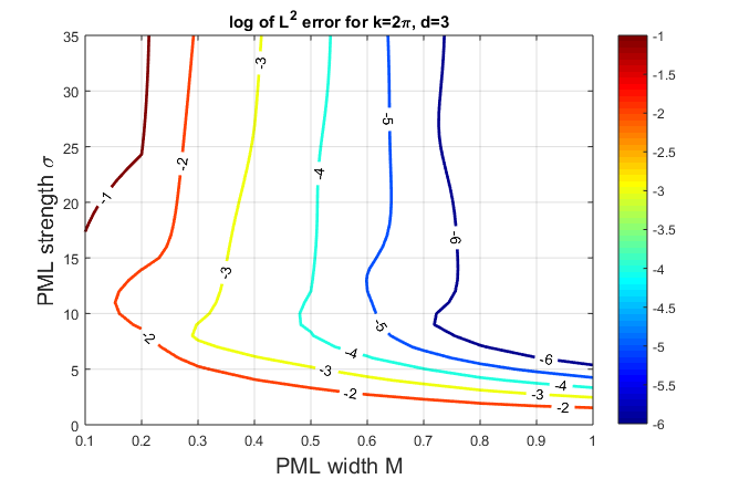
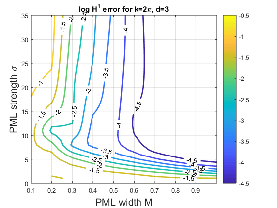
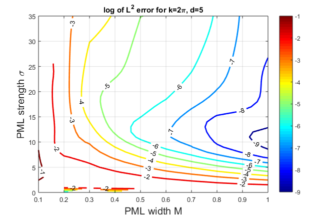
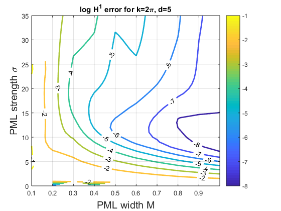
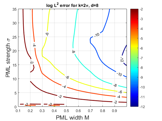
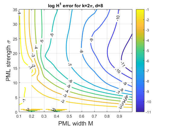
Figure 2: Contour plots for the $L^{2}$ and $H^{1}$ errors on a log scale for different PML strengths $\sigma_{0}$ and PML widths using splines of degrees $d=3,5,8$.

The results shown in Fig 8 illustrate that to attain a specified accuracy level, one can either increase the value of $\sigma_{0}$ or increase the size of the PML layer. For these examples, increasing the value of the PML strength above a certain threshhold does not improve the accuracy. In fact, in some cases the error gets worse with increasing $\sigma_{0}$. Results also show that higher order polynomial degrees require smaller PML sizes. For example for an $L^{2}$ accuracy of $10^{-6}$, the degree 3 splines require a PML width of 0.72 with $\sigma_{0}=10$, degree 5 splines require a PML width of 0.46 with $\sigma_{0}=12$, and the optimal PML width is 0.3 with $\sigma_{0}=20$ when the degree of the splines is 8. In all examples, one needs a larger PML size in order to attain higher accuracy.

6 Numerical Results

In this section, we present numerical results that demonstrate the performance of bivariate spline functions in solving the exterior Helmholtz problem (1). Our discretization seeks to approximate the solution of the PML problem (2).

For comparison with the PML solution, we also test the performance of the first order absorbing boundary condition, that is the solution of

$$-\Delta u-k^{2}u = f\;\hbox{ in }\Omega,$$

$$u = g\;\hbox{ on }\;\Gamma,$$

$$\dfrac{\partial u}{\partial n}-iku = 0\;\hbox{ on }\;\Gamma_{\!{}_{PML}}.$$ (33)

The Robin boundary condition on $\Gamma_{\!{}_{PML}}$ is a low order truncating boundary which can be added easily to a PML code. In fact, we approximate the Sommerfeld radiation condition by imposing the Robin boundary condition on the exterior boundary of the PML problem (2) and then set the PML parameter $\sigma_{0}=0$.

We choose the PML functions for $j=1,2$ as

$$\sigma_{j}(x_{j})=\left\{\begin{array}[]{@{}l@{\quad}l}0&\mbox{if $|x_{j}|<a_{j}$,}\\[3.0pt] \sigma_{0}\left(\dfrac{|x_{j}|-a_{j}}{b_{j}-a_{j}}\right)^{n}&\mbox{if $a_{j}\leq|x_{j}|\leq b_{j}$}\end{array}\right.$$

where $[-a_{1},a_{1}]\times[-a_{2},a_{2}]$ is the inner PML boundary, and $[-b_{1},b_{1}]\times[-b_{2},b_{2}]$ is the outer PML boundary. In all numerical experiments , we set $n=4$. Other choices of $n=0,1,2,3,5,\cdots$ or even unbounded functions (see [5, 6]) can be made, but preliminary numerical results suggest that the fourth order PML function considered here results a better accuracy. The errors are measured by the relative $L^{2}$ and $H^{1}$ norms on the triangulation $\Delta$ defined by

$$\mbox{L2error}=\dfrac{\|s_{\!{}_{\triangle}}-u\|_{L^{2}(\Delta)}}{\|u\|_{L^{2}(\Delta)}},\;\;\;\mbox{H1error}=\dfrac{\|\nabla(s_{\!{}_{\triangle}}-u)\|_{L^{2}(\Delta)}}{\|\nabla u\|_{L^{2}(\Delta)}},$$

where $s_{\!{}_{\triangle}}$ is the computed spline solution and $u$ the exact solution. In our computation, we actually use the discrete $\ell_{2}$ errors based on $500\times 500$ equally-spaced points over $[-b_{1},b_{1}]\times[-b_{2},b_{2}]$ exterior of $D$ to compute these relative errors above.

Example 1

Our first example is a detailed investigation of scattering of a plane wave from a disk $D_{2}$ of radius $a=2$ centered at the origin. We impose the PML layer inside the rectangular annulus $[-5,5]^{2}\setminus(-3,3)^{2}$. The computational region of interest for the problem is the annular region outside the circle $(-3,3)\setminus\overline{D_{2}}$. It is well known that if the plane wave is propagating along the positive $x$-axis ${\bf d}=(1,0)$, then the solution of the scattering problem can be expressed as a series of Hankel functions in polar coordinates

$$u(r,\theta) = -\left[\dfrac{J_{0}(ka)}{H_{0}^{(1)}(ka)}H_{0}^{(1)}(kr)+2\sum_{m=1}^{\infty}i^{m}\dfrac{J_{m}(ka)}{H_{m}^{(1)}(ka)}H_{m}^{(1)}(kr)\cos(m\theta)\right],$$ (34)

where $J_{m}(z)$ denotes the Bessel function of order $m$ and $H_{m}^{(1)}(z)$ is the Hankel function of the first kind and order $m$. In this example, a simple calculation verifies that $f=0$.

The incident field is a plane wave $\exp(ik{\bf x}\cdot{\bf d})$, and we take Dirichlet data on the boundary of the scatterer as

$$g({\bf x})=u(r,\theta)|_{\Gamma}.$$

Our choice of boundary data eliminates errors due to the approximation of the disk by regular polygons, since we are only interested in errors due to discretization and due to the PML. The minimal tolerance for the iterative method was set at $\varepsilon=10^{-10}$.

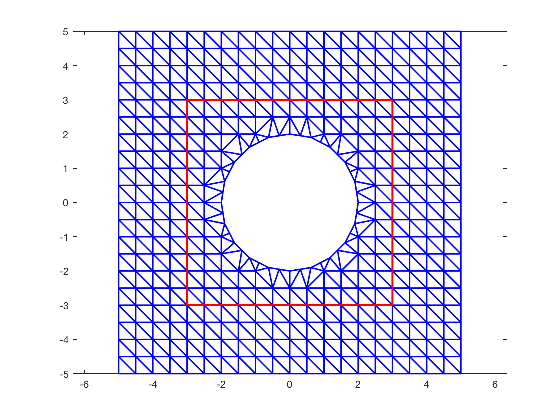
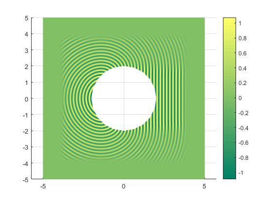
Figure 3: Meshes in Example 1 for $h=0.5$. Left: structured mesh aligned with inner PML boundary. Right: PML solution of the exterior Helmholtz equation with a wavenumber of $k=32$.

$h$	# dofs	PML $H^{1}$-error	PML $L^{2}$-error
1.000	3780	5.206370e-01	4.820429e-01
0.500	15120	3.428191e-02	1.821518e-02
0.333	33264	5.605999e-03	1.752080e-03
0.250	59220	1.292328e-03	2.777040e-04
0.200	92736	4.314135e-04	6.456502e-05

Table 1: Example 1.1: scattering from a disk, structured mesh PML solution with $\sigma_{0}=13$: $H^{1}$ and $L^{2}$ errors using fifth order splines $S^{1}_{5}(\Delta)$ for $h=1/\ell$, $\ell=1,2,3,4$ for $k=8$. The computational domain is the annular region outside a disk of radius 2, $[-3,3]^{2}\backslash\overline{D_{2}}$ and the PML layer is $[-5,5]^{2}\backslash(-3,3)^{2}.$

$d$	# dofs	PML $H^{1}$-error	ABC1 $H^{1}$ error	PML $L^{2}$-error	ABC1 $L^{2}$ error
5	15120	3.428191e-02	1.110241e-01	1.821518e-02	1.133321e-01
6	20160	4.833353e-03	9.584999e-02	1.555229e-03	1.006903e-01
7	25920	9.907632e-04	8.816546e-02	2.898009e-04	9.254443e-02
8	32400	1.196707e-04	8.274271e-02	2.746106e-05	8.680763e-02
9	39600	2.111239e-05	7.864768e-02	4.794616e-06	8.247796e-02
10	47520	2.013801e-06	7.541922e-02	5.266287e-07	7.906767e-02

Table 2: Example 1.2: scattering from a disk. Comparison of the PML and first order ABC on a structured mesh. $H^{1}$ and $L^{2}$ errors of spline solutions of various degrees $S^{1}_{d}(\Delta)$ for $d=5,6,7,8,9,10$, for wavenumber $k=8$ and meshwidth $h=0.5.$ The computational region of interest is the annular region outside a disk of radius 2, $[-3,3]^{2}\backslash\overline{D_{2}}$ and the PML layer is $[-5,5]^{2}\backslash(-3,3)^{2}$

EXAMPLE 1.1: The $h$-version
We first investigate convergence by refining a structured mesh uniformly so that $h=1,1/2,1/3,1/4,1/5$ while keeping the wavenumber fixed at $k=8$. Solutions are sought in the space $S^{1}_{5}(\Delta)$. Results are shown in Table 1. Both the $L^{2}$ and $H^{1}$ errors reduce by an order of magnitude with each refinement level. However the matrix size of the problem increases drastically with each uniform refinement, requiring $92736$ degrees of freedom for $h=0.2$ to reach an accuracy level of $4.3\times 10^{-2}\%$ error in the $H^{1}$ norm.

EXAMPLE 1.2: The $p$-version
Our next experiment investigates convergence when the polynomial degree $d$ is raised when $k=8$ and $h=0.5$ are fixed. Solutions are sought in the spaces $S^{1}_{d}(\Delta)$ for $d=5,6,7,8,9,10$. Results are presented in Table 2. In Table 2, we compare the PML solution with that of the first order absorbing boundary condition (see problem 6). As expected, the PML drastically outperforms the first order ABC. The error from the first order ABC stagnates at $7\%$ even using degree $10$ splines. This suggests that the dominant source of error is the ABC rather than the discretization, and the importance of accurate truncation of the exterior Helmholtz problem. Table 2 also shows that raising the degree of the splines rather than refining the mesh results in a significant reduction in the degrees of freedoms necessary to get a specified accuracy level. For example when $d=10$, the $H^{1}$ error is about $2\times 10^{-4}\%$ requiring $47520$ degrees of freedom.

$d$	# dofs	PML $H^{1}$-error	PML $L^{2}$-error
5	829,416	1.007229e+00	1.004805e+00
6	1,105,888	6.792040e-01	6.770829e-01
7	1,421,856	8.881512e-02	8.472434e-02
8	1,777,320	9.921788e-03	6.929828e-03
9	2,172,881	2.048858e-03	8.027105e-04
10	2,606,736	4.099069e-04	1.26832e-04

Table 3: Example 1.3: scattering from a disk, for a large wavenumber $k=100$, meshwidth $h=1/15$ on the domain in Figure 3. PML solution with $\sigma_{0}=13$: $H^{1}$ and $L^{2}$ errors using $S^{1}_{d}(\Delta)$ for $d=5,6,7,8,9,10.$

EXAMPLE 1.3: High Frequency Scattering
In the next experiment, the wavenumber is set at $k=100$, and the mesh is fixed at $h=1/15$ on the mesh in Figure 3. This is a high wavenumber, considering the characteristic length of the domain $kL\sim 800$. In Table 3, we investigate convergence of spline solutions to the Helmholtz scattering problem with $k=100$ in the spaces $S^{1}_{d}(\Delta)$ for polynomial degrees $d=5,6,7,8,9,10$. Results show good convergence at high wavenumber if $d$ is chosen large enough.

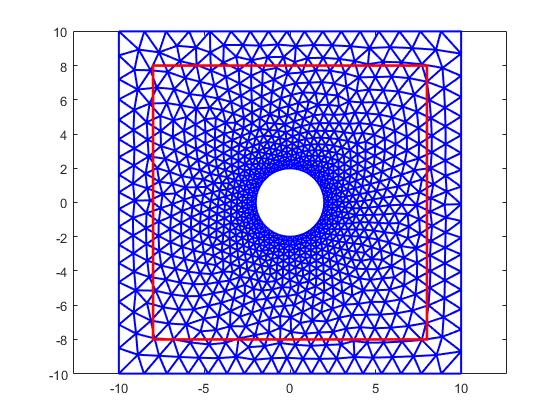
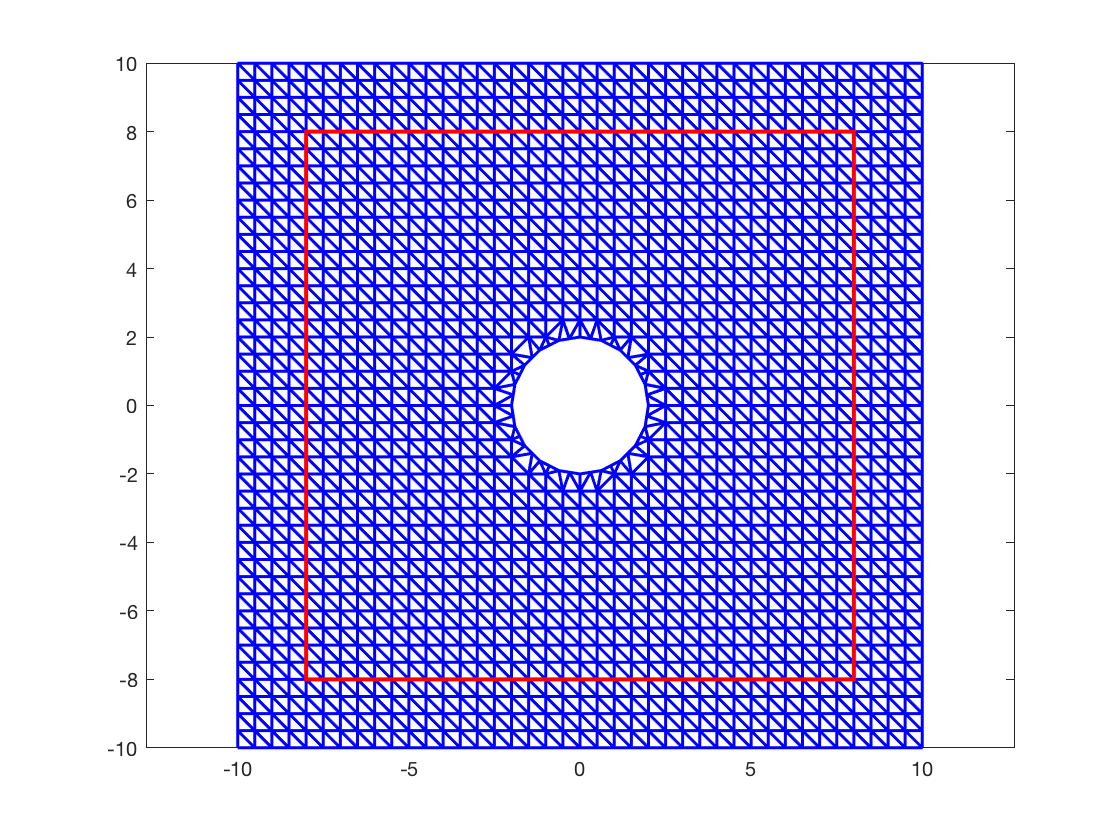
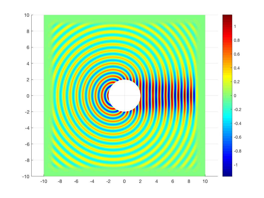
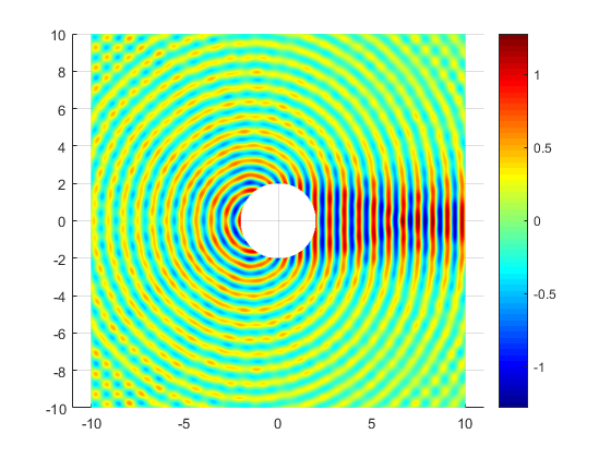
Figure 4: Top left: non-uniform mesh. Top right: uniform mesh. Bottom left: PML solution in $S^{1}_{8}(\Delta)$ for wavenumber $k=8$. Bottom right: First order ABC solution with a Robin boundary condition on the exterior boundary with wavenumber $k=8$. The effect of spurious reflections can be observed in the ABC solution.

$d$	# dofs	PML $H^{1}$-error	PML $L^{2}$-error
5	65520	5.631785e-02	4.420372e-02
6	87360	6.686595e-03	2.336916e-03
7	112320	1.214879e-03	3.377661e-04
8	140400	1.849320e-04	4.058609e-05
9	171600	2.635489e-05	5.472983e-06
10	205920	3.483980e-06	7.143510e-07

Table 4: convergence for scattering from a disk, uniform mesh with $h=0.5$. PML solution with $\sigma_{0}=13$: $H^{1}$ and $L^{2}$ errors using splines $S^{1}_{d}(\Delta)$ for $d=5,6,7,8,9,10$, wavenumber $k=8$. The computational domain is the annular region $(-8,8)^{2}\backslash[-2,2]^{2}$ and the PML layer is $[-10,10]^{2}\backslash(-8,8)^{2}.$

$d$	# dofs	PML $H^{1}$-error	PML $L^{2}$-error
5	42756	2.075821e-01	1.953157e-01
6	57008	7.687323e-02	7.205546e-02
7	73296	1.682735e-02	1.504267e-02
8	91620	3.660845e-03	2.922866e-03
9	111980	8.114318e-04	5.587460e-04
10	134376	2.211674e-04	1.501277e-04

Table 5: Example 1.4:$p$-version for a non-uniform mesh with $h=0.5$. PML solution with $\sigma_{0}=13$: $H^{1}$ and $L^{2}$ errors using $S^{1}_{d}(\Delta)$ for $d=5,6,7,8,9,10$, wavenumber $k=8$. The computational region of interest is the annular region $(-8,8)^{2}\backslash\overline{D_{2}}$ and the PML layer is $[-10,10]^{2}\backslash(-8,8)^{2}.$

EXAMPLE 1.4: A large domain
In Tables 4 and 5, the domain of the scattering problem is increased to the annulus $[-10,10]\setminus\overline{D_{2}}$, and the PML layer is set at $[-10,10]\setminus(-8,8)$, while the wavenumber is fixed at $k=8$. We test two cases of a structured mesh aligned with the PML boundaries and an unstructured mesh that cuts through the inner PML boundary. The unstructured mesh is graded so that the triangles in the PML layer are larger than triangles close to the scatterer, as shown in Figure 4. We only investigate convergence with respect to polynomial degree $d=5,6,7,8,9,10$ with a PML layer. Numerical results in Table 5 suggest good convergence even if the mesh is not aligned with the PML layer. There is a slight advantage to using unstructured meshes with larger triangles in the PML layer, with respect to the degrees of freedom required. An adaptive PML $hp$ procedure using error indicators is need to guarantee optimality with respect to mesh size and polynomial degrees.

Example 2

This example is taken from Table 1 of [23], where the authors use piecewise linear functions to solve a scattering problem with a PML layer. We are interested in using bivariate spline functions to solve this problem. This is an example of scattering of a spherical wave from a square $D=[-1,1]^{2}\subset\mathbb{R}^{2}$. The wavenumber is $k=2$, and the boundary condition on the surface of the scatterer is given by $g=e^{i\theta}H_{1}^{(1)}(kr)$. This implies that the exact solution is $u(r,\theta)=e^{i\theta}H_{1}^{(1)}(kr)$ in the exterior of $D$. Note that in this example $f=0$.

We choose the PML parameter $\sigma_{0}=13$. The region of computational interest is the annulus $(-3,3)^{2}\setminus[-1,1]^{2}$, and the PML layer is placed on $[-5,5]^{2}\setminus(-3,3)^{2}$. As in Table 1 of ([23]), we investigate convergence of the error in the $L^{2}$ and $H^{1}$ norms for different mesh sizes (see Figure 5).

EXAMPLE 2.1: Continuous Piecewise Linears
We first use continuous piecewise linears $S^{0}_{1}(\Delta)$ to replicate the results in Table 1 of ([23]) Results are shown in Table (6). We observe first order convergence in the $H^{1}$ norm and second order convergence in $L^{2}$ in agreement with the results in ([23]).

Figure 5: Meshes in Example 2 for $h=1,0.5$. The PML layer is outside the red boundary.

$h$	# dofs	PML $H^{1}$-error	ratio	PML $L^{2}$-error	ratio
1	576	0.882	0.00	0.601	0.000
1/2	2304	0.421	2.10	0.234	2.572
1/4	9216	0.192	2.19	0.0676	3.458
1/8	36864	0.0938	2.05	0.0174	3.891
1/16	147456	0.0463	2.03	0.00437	3.97

Table 6: Example 2.1: The $h$-version. PML solution with $\sigma_{0}=13$: $H^{1}$ and $L^{2}$ errors using linear splines $S^{0}_{1}(\Delta)$ for $h=1/2^{\ell}$, $\ell=0,1,2,3,4$ with exact solution $u(r,\theta)=e^{i\theta}H^{(1)}_{1}(kr)$ for $k=2$. The computational domain is the annular region $(-3,3)^{2}\backslash[-1,1]^{2}$ and the PML layer is $[-5,5]^{2}\backslash(-3,3)^{2}.$

EXAMPLE 2.2: The $p$ version
Next, we increase the degree of the spline spaces for a fixed mesh (we choose a course mesh $h=1$). The spline spaces $S^{1}_{d}(\Delta)\subset C^{1}(\Omega)$ are chosen with degree $d=5,6,7,8,9,10$. Results are shown in Table 7. Compared with the results in Table 6, we are able to obtain good accuracy with much fewer degrees of freedom on a relatively course mesh.

$d$	# dofs	PML $H^{1}$-error	ratio	PML $L^{2}$-error	ratio
5	4032	3.739715e-03	-	1.368041e-03	-
6	5376	1.901169e-03	1.97	1.040349e-03	1.31
7	6912	4.698431e-04	4.05	2.910898e-04	3.57
8	8640	1.488127e-04	3.16	1.162590e-04	2.50
9	10560	4.826350e-05	3.08	1.599918e-05	7.27
10	12672	4.742504e-05	1.02	4.377348e-05	0.37

Table 7: Example 2.2: The $p$-version. PML solution with $\sigma_{0}=13$: $H^{1}$ and $L^{2}$ errors of spline solutions of various degrees $S^{1}_{d}(\Delta)$ for $d=5,6,7,8,9,10$, with exact solution $u(r,\theta)=e^{i\theta}H^{(1)}_{1}(kr)$ for wavenumber $k=2$ and mesh width $h=1.$ The computational domain is the annular region $(-3,3)^{2}\backslash[-1,1]^{2}$ and the PML layer is $[-5,5]^{2}\backslash(-3,3)^{2}$.

Example 3

EXAMPLE 3.1: Helmholtz equation in a variable medium
In this section we illustrate the performance of bivariate splines for the variable media Helmholtz equation with a contrast function $b({\bf x})$ whose support is contained in $\Omega_{F}$.

$$-\Delta u({\bf x})-k^{2}(1-b({\bf x}))u({\bf x})=k^{2}b({\bf x})f({\bf x})\;\;\mbox{in}\;\;\Omega$$ (35)

$$u({\bf x})=g({\bf x})\;\;\mbox{on}\;\;\Gamma$$ (36)

satisfying the Sommerfeld radiation condition at infinity. This is similar to Example 4.1 of [1] where the source function is a plane wave. We use a point source incident field. The domain $\Omega=[-3,3]^{2}\backslash\overline{B}_{0.25}$ and $\Omega_{\rm PML}=[-3,3]^{2}\backslash(-2,2)^{2}$ where $B_{0.25}$ is a disk of radius 0.25 centered at the origin. We choose the contrast function as $b({\bf x})=0.5\;\mbox{erfc}(5(|{\bf x}|^{2}-1))$ where the error function $\mbox{erfc}(r)$ is defined by

$$\mbox{erfc}(r)=\dfrac{2}{\sqrt{\pi}}\int_{r}^{\infty}e^{-t^{2}}\;dt.$$

The function $b({\bf x})$ decays to zero quickly outside a bounded set (see Fig 6). We take the data function as $f({\bf x})=H_{0}^{(1)}(k|{\bf x}|)$, and choose Dirichlet data on $\Gamma$ as $g({\bf x})=u({\bf x})|_{\Gamma}$. The exact solution is then $u({\bf x})=H_{0}^{(1)}(k|{\bf x}|)$.

$d$	# dofs	PML $H^{1}$-error	PML $L^{2}$-error
5	49,770	2.521487e-03	1.703128e-03
6	66,360	5.461371e-04	4.989304e-04
7	85,320	1.630330e-04	1.677855e-04
8	106,650	6.051181e-05	6.425829e-05
9	130,350	1.688453e-05	1.756126e-05
10	156,420	7.292140e-06	7.701371e-06

Table 8: Example 3: Helmholtz equation in a variable medium. PML solution with $\sigma_{0}=10$: $H^{1}$ and $L^{2}$ errors of spline solutions of various degrees $S^{1}_{d}(\triangle)$ for $d=5,6,7,8,9,10$. The exact solution is $u({\bf x})=H_{0}^{(1)}(k|{\bf x}|)$ with $k=15$. The domain is shown in Figure 6.

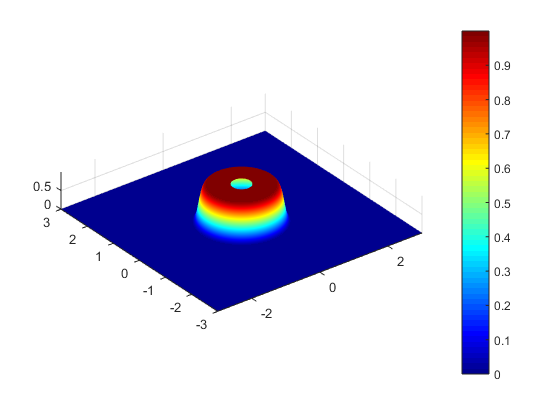
(a) Bump function $b({\bf x})=0.5\mbox{erfc}(5(|{\bf x}|^{2}-1))$.

(b) Mesh

Figure 6: The contrast function and mesh in Example 3.

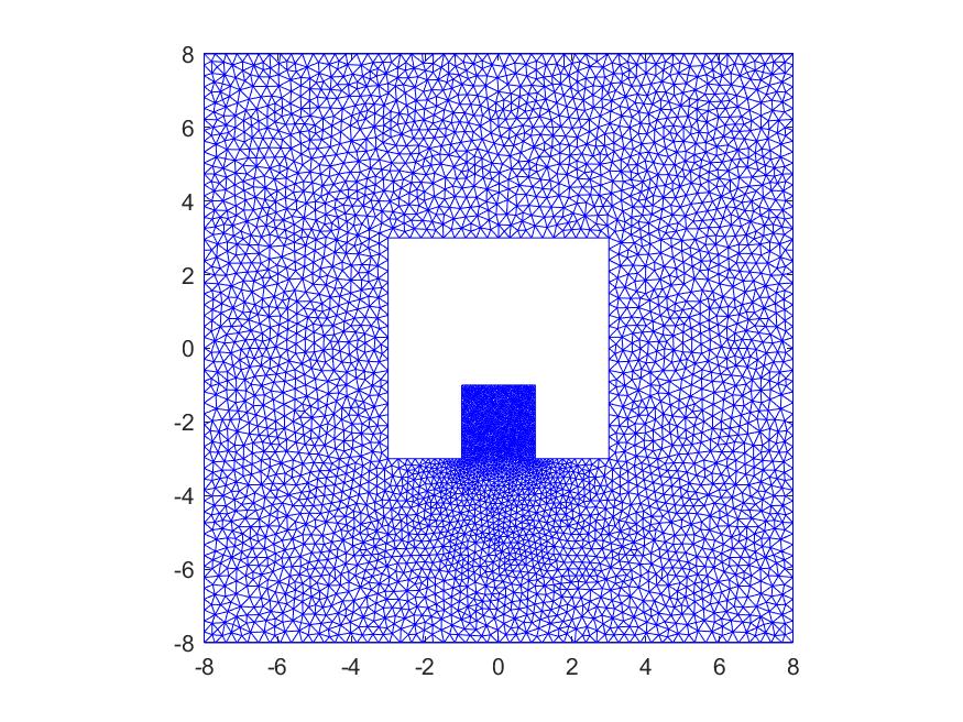
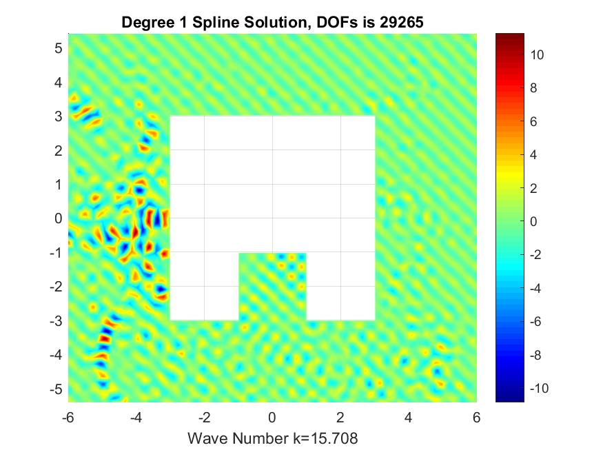
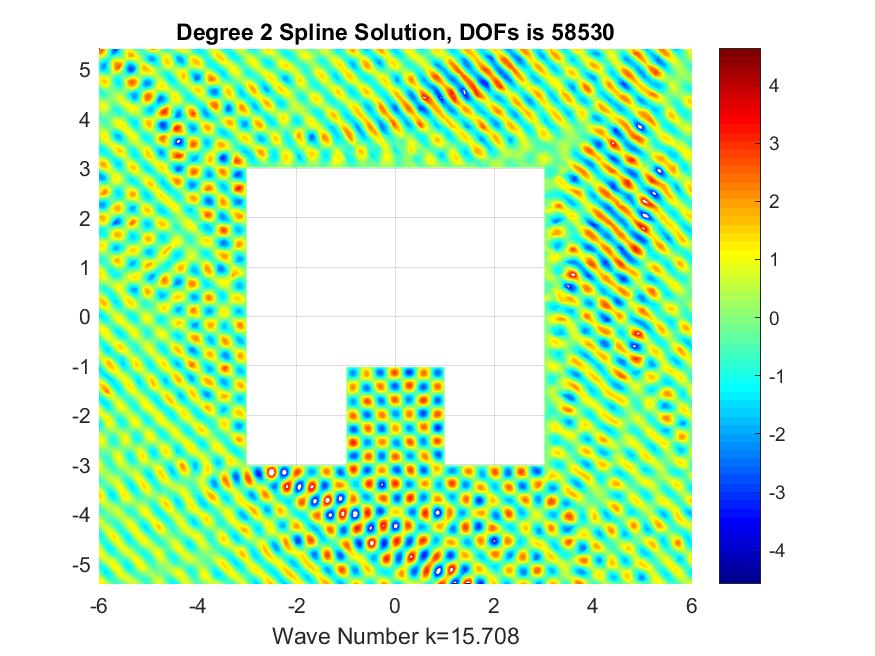
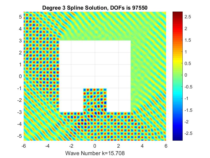
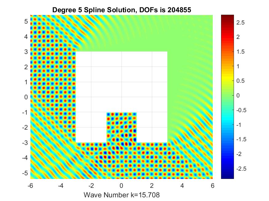
Figure 7: The truncated sound soft scattering problem using spline functions of degree $d=1,2,\cdots,5$. When $d\geq 3$, the resulting spline solution well resolves total wave (incident plus scattered).

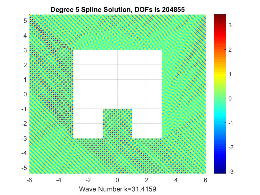
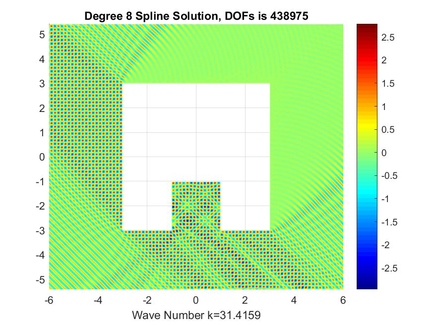
Figure 8: The truncated sound soft scattering problem using spline functions of degree $d=5$ and $d=8$. When $k=10\pi$, the spline solution of degree 5 does not produce an accurate approximation, but the spline solution of degree 8 does.

Example 4

This example is taken from [16] where the authors investigate the use of a pre-conditioner to solve the truncated sound soft scattering problem based on the shifted-Laplace equation. See [17] for another preconditioning approach. The domain and mesh are depicted in Figure 7 (top left panel). The outer boundary is a square of size $12\times 12$. The obstacle is a square of size $6\times 6$ placed symmetrically inside, with a $2\times 2$ square removed from the bottom side. We solve the truncated sound soft scattering problem with an incident plane wave coming from the bottom left corner of the graph, with the direction of propagation at 45 degrees with the positive $x$-axis. The scatterer in this example is trapping, since there exist closed paths of rays in its exterior. The researchers in [16] experimented the GMRES and used a preconditioner to find accurate solutions for various wave numbers $k$. From spline solutions of various degrees shown in Figure 7, we can see that when $d=1$ and $d=2$, the solutions are not accurate enough in the sense the waves are considerably less well resolved. When the spline degree is raised to $d\geq 3$, the solutions get better (see Figure 7), that is, the resulting total field (incident plus scattered) is well resolved. Even using bivariate spline functions of degree 5, the solution is generated within 200 seconds a laptop computer. Furthermore, for wave number $k=10\pi$, the degree 5 spline solution is not well-resolved as shown in Figure 8. However, when we use spline functions of degree 8, we are able to find a very accurate approximation. See the right graph of Figure 8. For large wave number, $k=500$ or larger, see the bivariate spline solution in [26].

Example 5

In our final numerical experiment, we investigate a “real life” example of the scattering of a point source located at one focus of an elliptic amphitheater (see Figure 9). We impose Dirichlet boundary conditions on the boundary of the elliptic walls associated with the point source and the fundamental solution of the Helmholtz equation

$$u({\bf x})|_{\!{}_{\Gamma}}=-\frac{i}{4}H_{0}^{(1)}(k|{\bf x}-{\bf x}_{0}|),$$

where ${\bf x}_{0}$ is the left focus of the inner ellipse. The inner and outer PML boundaries are the rectangles $[-2,2]^{2}$ and $[-2.2,2.2]^{2}$. In architectural acoustics, it is well known that a point source at the left focus leads to a maximum sound pressure at the right focus, in agreement with our results in Figure 9.

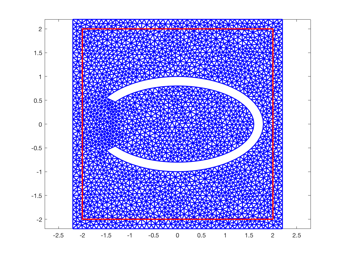
(a) Mesh for elliptic section with a PML layer.

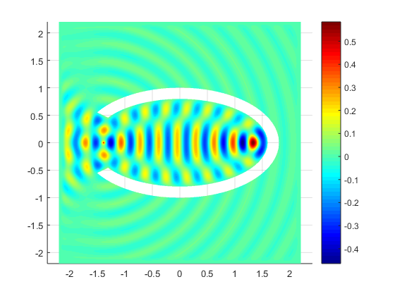
(b) real part of the PML solution, wavenumber $k=6\pi$

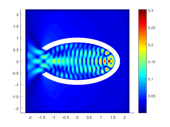
(c) modulus of the PML solution, wavenumber $k=6\pi$

Figure 9: Example 4: PML solution of acoustic wave propagation in a horizontal cross section of an elliptic amphitheater. A source at one focus leads to maximum sound pressure at the other focus.

7 Conclusion

We have shown how to approximate the solution of the exterior Helmholtz equation by using bivariate splines with a PML layer. Numerical results suggest good accuracy when using high order splines. Extension of our study to the Helmholtz equation in heterogeneous and anisotropic media will be reported elsewhere. Extension of the bivariate spline method to the 3D setting will be investigated in the near future.

References

- [1] Ambikarasan S., Borges C., Imbert-Gerard, L.-M., and Greengard, L., Fast, adaptive, high order accurate discretization of the Lippmann-Schwinger equation in two dimensions, SIAM J. Sci. Comput, 38, (2016) pp. A1770-A1787,
- [2] G. Awanou, M. J. Lai, P. Wenston, The multivariate spline method for numerical solution of partial differential equations, in Wavelets and Splines, Nashboro Press, Brentwood, 2006, pp. 24– 74.
- [3] J.P. Bérenger, A perfectly matched layer for the absorption of electromagnetic waves, J. Comput. Phys. 114 (1994) 185–200.
- [4] J.P. Bérenger, A perfectly matched layer for the FDTD solution of wave-structure interaction problems, IEEE T. Antennas and Propagation 44 (1996) 110–117.
- [5] A. Bermúdez, L. Hervella-Nieto, A. Prieto, R. Rodriguez, An exact bounded PML for the Helmholtz equation, C. R. Acad. Sci. Paris, Ser. I 339 (2004) 803–808.
- [6] A. Bermúdez, L. Hervella-Nieto, A. Prieto, R. Rodriguez, An exact bounded perfectly matched layer for time-harmonic scattering problems, SIAM J. Sci. Comput. 30 (1) (2007/2008) 312-338.
- [7] J. Bramble, J.E. Pasciak, Analysis of a Cartesian PML approximation to acoustic scattering problems in and , J. Comput. Appl. Math. 247, (2013), 209-230
- [8] G. Chen and J. Zhou, Boundary Element Methods, Academic Press Ltd, London, 1992
- [9] Z. Chen and X. Xiang A source transfer domain decomposition method for Helmholtz equations in unbounded domain, SIAM J. Numer. Anal. 51 (2013), 2331–2356.
- [10] Z. Chen and W. Zheng, Convergence of the uniaxial perfectly matched layer method for time-harmonic scattering problems in two-layered media, SIAM J. Numer. Anal. 48 (2010), 2158–2185.
- [11] W.C. Chew and W.H. Wheedon, A 3D Perfectly Matched Medium from Modified Maxwell’s equations with Stretched Coordinates, Microwave Opt. Technol. Lett., 7, pp. 599-604, 1994.
- [12] F. Collino, P. Monk The Perfectly Matched Layer in Curvilinear Coordinates, SIAM J. Sci. Comput. Vol 19, 6, pp. 2061-20190, 1998.
- [13] L. Evans, Partial Differential Equations, American Math. Society, Providence, 1998.
- [14] Floater, M. and Lai,M.-J.:Polygonal spline spaces and the numerical solution of the Poisson equation, SIAM J. Numer. Anal. 54, 797–824 (2016).
- [15] D. Givoli, Recent Advances in the DtN-FE method, J. Comput. Phys., Vol 122, pp.231-243, 1995.
- [16] M. J. Gander, J. G. Graham, and E. A. Spence, Applying GMRES to the Helmholtz equation with shifted Laplacian preconditioning: What is the largest shift for which wave number-independent convergence is guaranteed, Numer. Math., vol. 131, issue 3, page 567-614(2015).
- [17] J. G. Graham, E. A. Spence, and E. Vainikko, Domain decomposition decomposition preconditioning for high frequency Helmholtz problem with absorption, Math. Comp. vol. 86, Number 307, (2017), Pages 2089–2127.
- [18] J. Gutierrez, M.-J. Lai, G. Slavov: Bivariate spline solution of time dependent nonlinear PDE for a population density over irregular domains. Math. Biosci. 270, 263 -277 (2015)
- [19] W.S. Hall, The Boundary Element Method, Kluwer Academic Publishers, Group, Dordrecht, 1994
- [20] Y. He, D.P. Nicholls and J. Shen, An efficient and stable spectral method for electromagnetic scattering from a layered periodic structure. J. Comput. Phys., 231(8):3007-3022, 2012.
- [21] G. Hsiao, N. Nigam, J. Pasciak and L. Xu, Error Estimates for the DtN-FEM for the Scattering Problem in Acosutics, J. Comput. Appl. Math. Vol 235, 17, pp. 4949-4965, 2011
- [22] X. Hu, Han, D. and Lai, M. -J., Bivariate Splines of Various Degrees for Numerical Solution of PDE, SIAM Journal of Scientific Computing, vol. 29 (2007) pp. 1338–1354.
- [23] S. Kim and J. E. Pasciak, Analysis of a Cartesian PML approximation to acoustic scattering problems in , J. Math. Anal. Appl. 370 (2010) 168–186.
- [24] S. Kim, J.E. Pasciak, Analysis of the spectrum of a Cartesian perfectly matched layer (PML) approximation to acoustic scattering problems, J. Math. Anal. Appl. 361 (2) (2010) 420 -430.
- [25] M. -J., Lai, and Lanterman, J., A polygonal spline method for general 2nd order elliptic equations and its applications, in Approximation Theory XV: San Antonio, 2016, Springer Verlag, (2017) edited by G. Fasshauer and L. L. Schumaker, pp. 119–154.
- [26] M. -J. Lai and C. Mersmann, Bivariate Splines for Numerical Solution of Helmholtz Equation with Large Wave Number, under preparation, 2018.
- [27] M. -J. Lai and L. L. Schumaker, Spline Functions over Triangulations, Cambridge University Press, 2007.
- [28] M. -J. Lai and C. Wang, A Bivariate Spline Method for Second Order Elliptic Equations in Non-Divergence Form, Journal of Scientific Computing, (2018) pp. 803–829.
- [29] M. -J. Lai and Wenston, P., Bivariate Splines for Fluid Flows, Computers and Fluids, vol. 33 (2004) pp. 1047–1073.
- [30] M. Lassas and E. Somersalo, On the existence and convergence of the solution of PML equations, Computing, 60(3):229–241, 1998.
- [31] M. Lassas and E. Somersalo. Analysis of the PML equations in general convex geometry. Proc. Roy. Soc. Edinburgh Sect. A, 131(5):1183–1207, 2001.
- [32] N. N. Lebedev. Special functions and their applications. Revised English edition. Translated and edited by Richard A. Silverman. Prentice-Hall Inc., Englewood Cliffs, N.J., 1965.
- [33] Chao Liang and Xueshuang Xiang, Convergence of an Anisotropic Perfectly Matched Layer Method for Helmholtz Scattering Problems, Numer. Math. Theor. Meth. Appl. Vol. 9, No. 3, pp. 358–382 (2016)
- [34] J. Lin and H. Zhang, Scattering by a periodic array of subwavelength slits I: field enhancement in the diffraction regime, SIAM J. Multiscale Model. Sim., 16 (2018), 922-953.
- [35] J. Lin and H. Zhang, Scattering by a periodic array of subwavelength slits II: surface bound states, total transmission and field enhancement in homogenization regimes, SIAM J. Multiscale Model. Sim., 16 (2018), 954-990.
- [36] J. Lin and H. Zhang, Scattering and field enhancement of a perfect conducting narrow slit, SIAM J. Appl. Math., 77 (2017), 951-976.
- [37] D. Nicholls, N. Nigam, Error analysis of an enhanced DtN-FE method for exterior scattering problems, numer. Math., Vol 105, pp. 267-298, 2006.
- [38] D.P. Nicholls, Three-dimensional acoustic scattering by layered media: a novel surface formulation with operator expansions implementation. Proc. R. Soc. Lond. Ser. A Math. Phys. Eng. Sci., 468(2139):731–758, 2012.
- [39] L. L. Schumaker, Spline Functions: Computational Methods, SIAM Publication, 2015.
- [40] Joseph J. Shiron and Ivo Babuška, A Comparison of Approximate Boundary Conditions and Infinite Element Methods for Exterior Helmholtz problems, Comput. Methods Appl. Mech. Eng. Vol 164, No. 1-2, pp. 121-139 (1998).
- [41] A. Zarmi, E. Turkel, A general approach for high order absorbing boundary conditions for the Helmholtz equation, J. Comput. Phys., Vol 242, pp. 387-404, 2013.