Distributed Learning of Average Belief
Over Networks Using Sequential Observations

Abstract

This paper addresses the problem of distributed learning of average belief with sequential observations, in which a network of $n>1$ agents aim to reach a consensus on the average value of their beliefs, by exchanging information only with their neighbors. Each agent has sequentially arriving samples of its belief in an online manner. The neighbor relationships among the $n$ agents are described by a graph which is possibly time-varying, whose vertices correspond to agents and whose edges depict neighbor relationships. Two distributed online algorithms are introduced for undirected and directed graphs, which are both shown to converge to the average belief almost surely. Moreover, the sequences generated by both algorithms are shown to reach consensus with an $O({1}/{t})$ rate with high probability, where $t$ is the number of iterations. For undirected graphs, the corresponding algorithm is modified for the case with quantized communication and limited precision of the division operation. It is shown that the modified algorithm causes all $n$ agents to either reach a quantized consensus or enter a small neighborhood around the average of their beliefs. Numerical simulations are then provided to corroborate the theoretical results.

1 Introduction

Considerable interest in developing algorithms for distributed computation and decision making problems of all types has arisen over the past few decades, including consensus problems [2], multi-agent coverage problems [3], power distribution system management [4, 5], and multi-robot formation control [6]. These problems have found applications in different fields, including sensor networks [7], robotic teams [6], social networks [8], internet of things [9], and electric power grids [10, 4]. For large-scale complex networks, distributed computation and control are especially promising, thanks to their attractive features of fault tolerance and cost saving, and their ability to accommodate various physical constraints such as limitations on sensing, computation, and communication.

Among the distributed control and computation problems, the consensus problem [2, 11] is one of the most basic and important task. In a typical consensus process, the agents in a given group all try to agree on some quantity by communicating what they know only to their neighboring agents. In particular, one important type of consensus process, called distributed averaging [12], aims to compute the average of the initial values of the quantity of interest to the agents. Existing work has developed elegant solutions to such conventional distributed averaging problems, such as linear iterations [13]; gossiping [14, 15]; push-sum [16], also known as weighted gossip [17]; ratio consensus [18]; and double linear iterations [19].

In the present work, we extend the conventional distributed averaging problem setting to the case where each distributed agent has its local belief/measurement arriving sequentially. In the previous studies of distributed averaging, each agent $i$ was assumed to hold $x_{i}(1)$ at initial time $t=1$, which corresponds to the true belief, and the subsequent averaging and communication processes are carried out entirely over $x_{i}(1)$, $i\in\{1,2,\ldots,n\}$. In contrast, we consider here the case where a series of local observations, denoted by $x_{i}(t)$, $t\in\{1,2,\ldots\}$, is available to each agent $i$, which are used to estimate the unknown true belief $\bar{x}_{i}$. We refer to this setting as distributed learning of average belief using sequential observations.

Consider the motivating example of a sensor network, where each sensor needs to take a sequence of local measurements in order to obtain an accurate estimate of a local mean (or belief as referred to earlier) due to environmental and instrumentation noises; at the same time we have the goal of estimating the global/field mean through message exchange among sensors. It is clear that in this case there are multiple averaging processes taking place simultaneously, one globally among sensors, and a local one at each sensor. This is the main difference between our problem and traditional distributed averaging which only focuses on the global averaging process by assuming that the local mean is already available.

In general, the setting considered here belongs to the family of problems on distributed learning and control. We note that the distributed learning settings with noisy observations have also been investigated in several previous studies, e.g. [20, 7]. The key differences between our work here and those studies are the following: (1) in our formulation, uncertainties are not modeled as coming from external noise sources independent of the sample observations, as the case in the previous study [20]; (2) our algorithms are not developed based on a distributed estimation framework as in [7], where the observability of the system need to be assumed. Therefore, we note that there are multiple averaging processes going on simultaneously in our setting—a global one among the agents, and a local one at each agent. Similar ideas have been exploited in [21] and [22] for two different problems, distributed inference and estimation, respectively. In the classical literature on distributed averaging and consensus, however, only the global averaging process is considered since the local mean is already available. It would be desirable to embed the multiple underlying averaging processes here into the same updating procedure as in the classical distributed averaging process, without much modification. In particular, we should manage to integrate the new measurements/samples that occur in an online fashion into the classical distributed averaging process, which serves as the goal of the present work. To this end, we introduce two distributed online algorithms and formally establish their convergence and convergence rates.

To implement the algorithms, the agents are required to send, receive, as well as evaluate the running average of local beliefs with infinite precision. However, in a realistic network of agents, messages with only limited length are allowed to be transmitted among agents due to the capacity constraints of communication links. This is usually referred to as quantized communication in distributed averaging, see previous works on reaching quantized consensus under such quantization [23, 24, 25]. Additionally, in the distributed belief averaging algorithms considered here, limited precision of belief averages may occur due to the division operation in the local update at each agent. This is similar but more involved than the previous works on distributed averaging with integer/quantized values at each agent [11, 26, 27]. We thus discuss the convergence of the proposed algorithms in the presence of these two quantization effects. We can show that under certain conditions, the quantized update can converge to a small neighborhood of the actual average belief with bounded errors, even with such joint quantization effects.

The main contributions of this paper are threefold. First, we propose a new setting of distributed averaging using sequential observations, and develop two easily-implementable distributed algorithms for undirected and directed graphs, respectively. Second, we establish almost sure convergence and polynomial convergence rate with high probability for both algorithms. In addition, we investigate the effects of quantized communication and limited precision of the division operation on the algorithm for undirected graphs, and provide a convergence analysis under certain conditions.

This paper builds on some earlier results presented in [1], but presents a more comprehensive treatment of the problem. Specifically, the paper establishes the convergence rate for the algorithm over directed graphs, and characterizes the effects of two types of quantization on the algorithm over undirected graphs, which were not included in [1].

The rest of the paper is organized as follows. The problem is formulated and stated in Section 2. Two algorithms are presented to solve the problem over undirected and directed graphs, in Section 3, along with results on their convergence rates. In Section 4, the convergence results for the algorithm under system quantization are provided, for both static and dynamic graphs. The analysis of the algorithms and proofs of the main results are given in Section 5. The theoretical results are verified by numerical simulations in Section 6, followed by conclusions in Section 7.

2 Problem Formulation

Consider a network consisting of $n>1$ agents, with the set of agents denoted by $\mathcal{N}=\{1,2,\cdots,n\}$. The neighbor relationships among the $n$ agents are described by a time-varying $n$-vertex graph $\mathbb{N}(t)=\left(\mathcal{N},{\mathcal{E}}(t)\right)$, called the neighbor graph, with ${\mathcal{E}}(t)$ denoting the set of edges at time $t$. Note that the graph $\mathbb{N}(t)$ can be either undirected or directed. The $n$ vertices represent the $n$ agents and the edges indicate the neighbor relationships. Specifically, if the communications among agents are bidirectional, the graph $\mathbb{N}(t)$ is undirected, and agents $i$ and $j$ are neighbors at time $t$ if and only if $(i,j)$ is an edge in $\mathbb{N}(t)$. We use ${\mathcal{N}}_{i}(t)$ to denote the set of neighbors of agent $i$, i.e., the degree of vertex $i$ at time $t$. We also define ${\mathcal{N}}_{i}^{+}(t):=\mathcal{N}_{i}(t)\bigcup\{i\}$ as the set of neighbors including the agent $i$ itself. Otherwise, if the communications are unidirectional, we say that an agent $j$ is an out-neighbor of agent $i$ at time $t$ if agent $i$ can send information to agent $j$ at time $t$. In this case, we also say that agent $i$ is an in-neighbor of agent $j$ at time $t$. Then, agent $j$ is a out-neighbor of agent $i$ (and thus agent $i$ is an in-neighbor of agent $j$) at time $t$ if and only if $(i,j)$ is a directed edge in $\mathbb{N}(t)$. Thus, the neighbor graph $\mathbb{N}(t)$ becomes directed, in which the directions of edges represent the directions of information flow. By a slight abuse of notation, we use ${\mathcal{N}}_{i}(t)$ to denote the set of out-neighbors of agent $i$ at time $t$, and also let ${\mathcal{N}}_{i}^{+}(t)={\mathcal{N}}_{i}(t)\bigcup\{i\}$. We also use $o_{i}(t)$ to denote the number of out-neighbors of agent $i$ at time $t$, or equivalently, the out-degree of vertex $i$ in $\mathbb{N}(t)$.

We assume that time is discrete in that $t$ takes values in $\{1,2,\ldots\}$. Each agent $i$ receives a real-valued scalar $x_{i}(t)$ at each time $t$. We assume that the samples $\{x_{i}(t)\}_{t=1}^{\infty}$ form an independent and identically distributed (i.i.d.) process, and the sequence is generated according to a random variable $X_{i}$ with distribution $f_{X_{i}}(\cdot)$. For simplicity, we assume that the support set for $X_{i}$ is bounded, i.e., there exists a constant $K$ such that $|X_{i}(\omega)|\leq K$ for all $i\in{\mathcal{N}}$ and $\omega$, where $\omega$ indicates an arbitrary sample realization. Note that the agents’ observations do not need to be identical, i.e., the $f_{X_{i}}(\cdot)$, $i\in{\mathcal{N}}$, do not need to be structurally the same. We use $\bar{x}_{i}$ to denote the expectation of agent $i$’s local observations, i.e.,

$$\bar{x}_{i}=E[X_{i}]~{},$$

and call $\bar{x}_{i}$ the local belief of agent $i$. An application context for this problem in sensor networks was described in the introduction as a motivating example.

At each time step $t$, each agent $i$ can exchange information only with its current neighbors $j\in\mathcal{N}_{i}(t)$. Thus, only local information is available to each agent, i.e., each agent $i$, only knows its own samples, the information received from its current neighbors in $\mathcal{N}_{i}(t)$, and nothing more, while the global connectivity patterns remain unknown to any agent in the network.

Suppose that each agent has control over a real-valued variable $y_{i}(t)$ which it can update from time to time. Let

$$\bar{x}=\frac{1}{n}\sum_{i=1}^{n}\bar{x}_{i}~{},$$ (1)

represent the average belief within the network. Our goal is to devise distributed algorithms for each agent $i$, over either undirected or directed graphs, which ensures that

$$\lim_{t\rightarrow\infty}y_{i}(t)=\bar{x}~{},\;\;\;\;\;\forall i~{},$$

almost surely (a.s.). Moreover, we would like to characterize the convergence properties of such algorithms with high probability (w.h.p.), and their extensions to the case with quantization effects of the system, as we will elaborate next.

3 Distributed Learning Algorithms

In this section, we introduce two algorithms for distributed learning of average belief using sequential observations over time-varying graphs. We establish both almost sure convergence and ${O}(1/t)$ convergence rate w.h.p. for the algorithms.

3.1 Algorithms

We first consider the case where $\mathbb{N}(t)$ is a time-varying undirected graph. At initial time $t=1$, each agent $i$ sets $y_{i}(1)=x_{i}(t)$, where we note that $x_{i}(t)$ is an i.i.d. sample of the local belief ${X}_{i}$. For each time $t>1$, each agent $i$ first broadcasts its current $y_{i}(t)$ to all its current neighbors in ${\mathcal{N}}_{i}(t)$. At the same time, each agent $i$ receives $y_{j}(t)$ from all its neighbors $j\in{\mathcal{N}}_{i}(t)$. Then, each agent $i$ updates its variable by setting

$$y_{i}(t+1) = w_{ii}(t)y_{i}(t)+\sum_{j\in{\mathcal{N}}_{i}(t)}w_{ij}(t)y_{j}(t)$$ (2)

$$+z_{i}(t+1)-z_{i}(t)~{},$$

where

$$z_{i}(t)=\frac{1}{t}\sum_{\tau=1}^{t}x_{i}(\tau)$$ (3)

is the running average of the data, and $w_{ij}(t)$ is the real-valued weight from the matrix $W(t)=[w_{ij}(t)]\in\mathbb{R}^{n\times n}$. The update rule (2) can be written in a more compact form as

$$y(t+1)=W(t)y(t)+z(t+1)-z(t)~{},$$ (4)

where $y(t),z(t)\in\mathbb{R}^{n}$ are the column vectors obtained by stacking up $y_{i}(t)$s and $z_{i}(t)$s, respectively.

We make the following standard assumptions on $W(t)$ hereafter unless stated otherwise.

Assumption 1.

The weight matrix $W(t)$ has the following properties at any time $t$.

A.1) $W(t)$ is a symmetric stochastic matrix with positive diagonal entries, i.e., $\forall i,j\in{\mathcal{N}}$,

$$w_{ii}(t)>0,\;w_{ij}(t)=w_{ji}(t)\geq 0,\;\text{and}$$

$$\sum_{k=1}^{n}w_{kj}(t)=\sum_{k=1}^{n}w_{ik}(t)=1~{}.$$

A.2) $W(t)$ is consistent with the network connectivity constraint, i.e., if $(i,j)\notin{\mathcal{E}}(t)$, then $w_{ij}(t)=0$. $\Box$

Note that Assumption 1 is a standard one for the conventional distributed averaging problem (without any sequential observations) [23]. Such weights $w_{ij}(t)$ can be designed in a distributed manner using the well-known Metropolis weights [13].

Moreover, note that even though $z_{i}(t)$ used in the update is a running average over time, an agent need not store all its received samples. Instead, each agent $i$ can only keep track of $z_{i}(t)$ and update following

$$z_{i}(t+1)=\frac{tz_{i}(t)+x_{i}(t+1)}{t+1}~{}.$$ (5)

The algorithm (2) requires that the communication between any pair of neighboring agents be bidirectional. Such a requirement may not always be satisfied in applications. For example, different agents may have distinct transmission radii. In this subsection, we introduce another algorithm to handle the case when the neighbor graph $\mathbb{N}(t)$ is directed, i.e., the communication between agents is unidirectional. The algorithm makes use of the idea of the push-sum protocol [16], which solves the conventional distributed averaging problem for directed neighbor graphs.

Now, we consider the following algorithm (for directed neighbor graphs). Each agent $i$ has control over two real-valued variables $y_{i}(t)$ and $v_{i}(t)$, which are initialized as $y_{i}(1)=x_{i}(1)$ and $v_{i}(1)=1$, respectively. At each time $t>1$, each agent $i$ sends the weighted current values $\frac{y_{i}(t)}{1+o_{i}(t)}$ and $\frac{v_{i}(t)}{1+o_{i}(t)}$ to all its current neighbors and updates its variables according to the rules

$${\color[rgb]{0,0,0}\mu_{i}}(t+1) =\frac{y_{i}(t)}{1+o_{i}(t)}+\sum_{j\in{\mathcal{N}}_{i}(t)}\frac{y_{j}(t)}{1+o_{j}(t)}~{},$$

$$v_{i}(t+1) =\frac{v_{i}(t)}{1+o_{i}(t)}+\sum_{j\in{\mathcal{N}}_{i}(t)}\frac{v_{j}(t)}{1+o_{j}(t)}~{},$$

$$y_{i}(t+1) ={\color[rgb]{0,0,0}\mu_{i}}(t+1)+z_{i}(t+1)-z_{i}(t)~{},$$ (6)

where $o_{i}(t)$ denotes the number of observers at agent $i$ at time $t$, and $z_{i}(t)$ is the running average as defined in (3). The quotient ${{\color[rgb]{0,0,0}\mu_{i}}(t)}/{v_{i}(t)}$ can then be shown to converge to $\bar{x}$.

3.2 Convergence Results

To establish convergence results, we first introduce some concepts on the connectivity of time-varying graphs. An undirected graph $\mathbb{G}$ is called connected if there is a path between each pair of distinct vertices in $\mathbb{G}$. A directed graph $\mathbb{G}$ is called strongly connected if there is a directed path between each ordered pair of distinct vertices in $\mathbb{G}$. By the union of a finite sequence of undirected (or directed) graphs, $\mathbb{G}_{1},\mathbb{G}_{2},\ldots,\mathbb{G}_{p}$, each with the vertex set ${\mathcal{V}}$, is meant the undirected (or directed) graph $\mathbb{G}$ with vertex set ${\mathcal{V}}$ and edge set equaling the union of the edge sets of all the graphs in the sequence. We say that such a finite sequence is jointly connected (or jointly strongly connected) if the union of its members is a connected (or strongly connected) graph. We say that an infinite sequence of undirected (or directed) graphs $\mathbb{G}_{1},\mathbb{G}_{2},\ldots$ is repeatedly jointly connected (or repeatedly jointly strongly connected) if there is a positive integer $r$ such that for each $k\geq 0$, the finite sequence $\mathbb{G}_{rk+1},\mathbb{G}_{rk+2},\ldots,\mathbb{G}_{r(k+1)}$ is jointly connected (or jointly strongly connected).

Now we are ready to present the connectivity assumption on the undirected neighbor graphs $\{\mathbb{N}(t)\}$, building upon which we establish the convergence of system (4).

Assumption 2.

The sequence of undirected neighbor graphs $\{\mathbb{N}(t)\}$ is repeatedly jointly connected. $\Box$

Theorem 1.

Let all $n$ agents adhere to the update rule (2). Suppose that Assumptions 1 and 2 hold. Then,

$$\lim_{t\rightarrow\infty}y_{i}(t)=\bar{x}~{},\;\;\;\;\;\forall i,$$ (7)

almost surely. Moreover, the sequence $\{y_{i}(t)\}$ reaches consensus for all $i\in\mathcal{N}$ with the order of $O({1}/{t})$ w.h.p. $\Box$

A precise proof of the theorem is relegated to Section 5, but here we provide the basic intuition behind it. First, it is straightforward to verify that

$$\lim_{t\rightarrow\infty}\frac{1}{n}\sum_{i=1}^{n}z_{i}(t)=\frac{1}{n}\sum_{i=1}^{n}\bar{x}_{i}~{}.$$ (8)

Since $y(1)=x(1)=z(1)$, from (4), it follows that $\mathbf{1}^{\top}y(2)=\mathbf{1}^{\top}z(2)$, where $\mathbf{1}$ denotes the vector whose entries all equal to $1$ and $\mathbf{1}^{\top}$ denotes its transpose. By induction, it follows that $\mathbf{1}^{\top}y(t)=\mathbf{1}^{\top}z(t)$ for any $t$, which implies by ignoring the small perturbation terms $z(t+1)-z(t)$ (later we will show that this term converges polynomially fast to the zero vector $\mathbf{0}$ w.h.p.), $y(t+1)=W(t)y(t)$ leads all $y_{i}(t)$ to the same value [23]. Note that, from (8) and (1), $\sum_{i=1}^{n}z_{i}(t)$ will converge to $n\bar{x}$, and therefore we could expect that each $y_{i}(t)$ will converge to $\bar{x}$ since $\mathbf{1}^{\top}y(t)=\mathbf{1}^{\top}z(t)$.

Likewise, we impose the following assumption on the connectivity of the neighbor graph $\mathbb{N}(t)$ when it is directed.

Assumption 3.

The sequence of directed neighbor graphs $\{\mathbb{N}(t)\}$ is repeatedly jointly strongly connected. $\Box$

Now we are ready to present the convergence result for the update rule (6) for directed neighbor graphs, which shows that it also achieves the same convergence result as update rule (4) for undirected neighbor graphs.

Theorem 2.

Let all $n$ agents adhere to the update rule (6). Suppose that Assumptions 1 and 3 hold. Then,

$$\lim_{t\rightarrow\infty}\frac{{\color[rgb]{0,0,0}\mu_{i}}(t)}{v_{i}(t)}=\bar{x}~{},\;\;\;\;\;\forall i~{},$$ (9)

a.s. Moreover, the sequence $\{{{\mu_{i}}(t)}/{v_{i}(t)}\}$ reaches consensus for all $i\in\mathcal{N}$ with the order of $O({1}/{t})$ w.h.p. $\Box$

Proof of this theorem is given later in Section 5.

Based on Theorems 1 and 2, we also obtain the following corollary which quantifies the convergence performance of the update rules for a finite time $t$. The proof is deferred to Section 5.

Corollary 1.

For the update (2), there exist constants $\lambda_{1}\in[0,1)$ and $C_{1},C_{2}>0$, such that after $t\geq(2C_{2})^{-1}\cdot\log\left(\frac{2}{\delta(1-2e^{-2C_{2}})}\right)$ iterations,

$$|y_{i}(t)-\bar{x}|\leq C_{1}\lambda_{1}^{t}+({C_{2}+K+\bar{x}_{i}})/{t},~{}~{}\forall i\in{\mathcal{N}}~{}~{}$$

holds with probability at least $1-\delta$. The same finite-time performance also holds for the update (6).

4 Quantization Effects

In this section, we investigate the effects of two common sources of quantization on algorithm (2). Specifically, the quantization includes quantized communication and limited precision of the division operation, which are common in realistic distributed computation systems. The joint effects of the two quantization are considered over both static and dynamic neighbor graphs.

4.1 Static Graphs

The algorithm (2) requires the agents to send and receive real-valued variables $y(t)$ at each iteration. However, in a realistic network, with limited capacity of communication links, the messages transmitted among agents can have only limited length. On the other hand, both updates (3) and (5) require one step of division operation. As such, the result $z(t)$ may only have limited precision due to the finite digits of representing divided numbers in realistic digital computers. This effect can be viewed as one type of quantization on the value of $z(t)$. With these two quantization effects, the precise belief averaging cannot be achieved in general (except in some special cases). We first analyze the performance of system (4) subject to these effects over a static neighbor graph. To this end, we impose the following standard assumption on the static graph and the corresponding weight matrix.

Assumption 4.

The communication graph $\mathbb{N}(t)$ is static and connected, i.e., $\mathbb{N}(t)=({\mathcal{N}},{\mathcal{E}})$ for all $t$ where $({\mathcal{N}},{\mathcal{E}})$ is a connected undirected graph. Accordingly, there exists a matrix $W$ which satisfies Assumption 1 in that $W(t)=W$ for all $t$, and has the following properties:

A.1) $W$ has dominant diagonal entries, i.e., $w_{ii}>1/2$ for all $i\in{\mathcal{N}}$.

A.2) For any $(i,j)\in{\mathcal{E}}$, we have $w_{ij}\in\mathbb{Q}^{+}$, where $\mathbb{Q}^{+}$ is the set of rational numbers in the interval $(0,1)$. $\Box$

Note that conditions A.1) and A.2) are specifically needed for the convergence of quantized systems as in [25]. In a practical implementation, it is not restrictive to have rational numbers as weights and require dominant diagonal weights. As reported in [25, Appendix A], the quantized update may fail to converge even in the deterministic setting of distributed averaging. Thus, conditions A.1) and A.2) are essential here since our analysis will rely on the results developed in [25].

Let $\tilde{z}_{i}(t)$ denote the value of $z(t)$ after the division in (3), or equivalently (5). We impose an assumption on $\tilde{z}_{i}(t)$ as follows.

Assumption 5.

There exists a precision $\Delta>0$ such that $\tilde{z}_{i}(t)$ is multiples of $\Delta$ for any time $t$ and $i\in{\mathcal{N}}$. $\Box$

It follows from Assumption 5 that the decimal part of $\tilde{z}_{i}(t)$ can only have a finite number of values. For notational convenience, we introduce the following definitions. Define the sets ${\mathcal{B}}$ and ${\mathcal{C}}$ as,

$${\mathcal{B}}:=\{b:b=k\Delta+\Delta/2,k=0,1,\cdots\},$$ (10)

$${\mathcal{C}}:=\{b:b=k\Delta,k=0,1,\cdots\}.$$ (11)

Let ${\mathcal{R}}:\mathbb{R}\to\mathbb{R}$ be the operation that rounds the value to the nearest multiples of $\Delta$, i.e.,

$${\mathcal{R}}(x)=\mathop{\mathrm{argmin}}_{b\in{\mathcal{C}}}|b-x|.$$ (12)

Hence, we have $\tilde{z}_{i}(t)={\mathcal{R}}(z_{i}(t))$. In particular, if $x\in{\mathcal{B}}$ for some $k>0$, we define the value of ${\mathcal{R}}(x)$ as ${\mathcal{R}}(x):=(k+1)\Delta$. In practice, the value of the quantized $\tilde{z}_{i}(t)$ can be evaluated by simply keeping track of the summation of all the previous data at time $t$, i.e., define $s_{i}(t):=\sum_{\tau\leq t}x_{i}(\tau)$, and then calculate $\tilde{z}_{i}(t)={\mathcal{R}}(s_{i}(t)/t)$. In this regard, the imprecision caused by the division operation will not accumulate over time.

To avoid the information loss caused by the quantized communication, we adopt the following update:

$$y(t+1)=W{\mathcal{Q}}(y(t))+y(t)-{\mathcal{Q}}(y(t))+\Delta\tilde{z}(t+1)~{},$$ (13)

where ${\mathcal{Q}}:\mathbb{R}^{n}\to\mathbb{R}^{n}$ denotes the operation of element-wise quantization on a vector, and $\Delta\tilde{z}(t+1):=\tilde{z}(t+1)-\tilde{z}(t)$. The deterministic quantizer ${\mathcal{Q}}$ can be either truncation quantizer ${\mathcal{Q}}_{t}$, the ceiling quantizer ${\mathcal{Q}}_{c}$, or the rounding quantizer ${\mathcal{Q}}_{r}$, which round the values to, respectively, the nearest lower integer, the nearest upper integer, or the nearest integer. For more discussion on the types of deterministic quantizers, see [25, Section IV]. Without any loss of generality, we analyze the system with a truncation quantizer ${\mathcal{Q}}_{t}$.

Since $W$ is column stochastic (i.e., $\mathbf{1}^{\top}W=\mathbf{1}^{\top}$), from equation (13), we have

$$\mathbf{1}^{\top}y(t+1)=\mathbf{1}^{\top}y(t)+\mathbf{1}^{\top}\big{(}\tilde{z}(t+1)-\tilde{z}(t)\big{)}.$$ (14)

Hence, the property that $\mathbf{1}^{\top}y(t)=\mathbf{1}^{\top}\tilde{z}(t)$ for any $t$ also holds under quantized communication provided $\mathbf{1}^{\top}y(1)=\mathbf{1}^{\top}\tilde{z}(1)$. In addition, we define $m(t)$ and $M(t)$ as follows:

$$m(t):=\min_{i\in{\mathcal{N}}}\lfloor y_{i}(t)\rfloor,~{}~{}~{}M(t):=\max_{i\in{\mathcal{N}}}\lfloor y_{i}(t)\rfloor,~{}~{}\forall t\geq 0~{},$$

where $\lfloor\cdot\rfloor$ denotes the floor function. Let $\alpha_{i}=1-w_{ii}+\gamma$, and $\gamma>0$ be a sufficiently small positive scalar that guarantees $\alpha_{i}<0.5$. As shown in [25], the value of $\gamma$ is not necessarily known and is only used here for the convenience of analysis. Define $\alpha:=\max\limits_{i\in{\mathcal{N}}}\alpha_{i}$, which is also upper bounded by $0.5$, and a value $\bar{x}_{{\mathcal{R}}}$ as

$$\bar{x}_{{\mathcal{R}}}:=\frac{1}{n}\sum_{i\in{\mathcal{N}}}{\mathcal{R}}(\bar{x}_{i})~{}.$$ (15)

If $\bar{x}_{i}\notin{\mathcal{B}},\forall i\in{\mathcal{N}}$, then the value of $\bar{x}_{{\mathcal{R}}}$ corresponds to the average of all beliefs with limited precisions. Note that the difference between $\bar{x}_{{\mathcal{R}}}$ and the actual average belief $\bar{x}$ is no greater than $\Delta/2$ by definition. We will show that the quantized system (13) will converge to the neighborhood of $\bar{x}_{{\mathcal{R}}}$ a.s., provided that $\bar{x}_{i}\notin{\mathcal{B}},\forall i\in{\mathcal{N}}$. Formally, we have the following proposition on the convergence of system (13).

Proposition 1.

Let all $n$ agents adhere to the update rule (13). Under Assumptions 4 and 5, if $\bar{x}_{i}\notin{\mathcal{B}},\forall i\in{\mathcal{N}}$, then almost surely either

1) the system reaches quantized consensus to the value $\bar{x}_{{\mathcal{R}}}$ defined in (15), i.e.,

$$\left\{\begin{array}[]{ll}\lfloor y_{i}(t)\rfloor=\lfloor y_{j}(t)\rfloor,\;\forall i,j\in{\mathcal{N}}~{},\\ |y_{i}(t)-\bar{x}_{{\mathcal{R}}}|<1,\;\forall i\in{\mathcal{N}}~{},\end{array}\right.$$

which implies that $|y_{i}(t)-\bar{x}|<1+{\Delta}/{2},\forall i\in{\mathcal{N}}$, or

2) all $n$ agents’ values live in a small neighborhood around $\bar{x}_{{\mathcal{R}}}$ in that

$$\left\{\begin{array}[]{ll}|y_{i}(t)-y_{j}(t)|\leq\alpha_{i}+\alpha_{j},\;\forall i,j\in{\mathcal{N}}~{},\\ |y_{i}(t)-\bar{x}_{{\mathcal{R}}}|\leq 2\alpha,\;\forall i\in{\mathcal{N}}~{},\end{array}\right.$$

which implies that $|y_{i}(t)-\bar{x}|<2\alpha+{\Delta}/{2},\forall i\in{\mathcal{N}}$. $\Box$

Proposition 1 states that under the condition that $\bar{x}_{i}\notin{\mathcal{B}},\forall i\in{\mathcal{N}}$, system (13) will either reach a quantized consensus with error smaller than $1+{\Delta}/{2}$ to the actual average belief $\bar{x}$, or enter a bounded neighborhood of $\bar{x}$ with size smaller than $2\alpha+{\Delta}/{2}$. This result can be viewed as extension of the one for standard distributed averaging with quantized communications [25]. Notably, the quantization effect caused by the division operation enlarges the error away from exact consensus by an amount of ${\Delta}/{2}$, which is usually small in practice. The proof of the proposition is provided in Section 5.

Remark 1.

It is worth noting that the limiting behavior of the quantized system (13) differs from the results in [25] in three ways: i) quantized communication does not necessarily cause exact cyclic behavior of $y(t)$ due to the randomness in the sequential data sample $x_{i}(t)$; ii) limited precision of $\tilde{z}(t)$ induces inevitable mismatch to the convergent point from the actual average belief $\bar{x}$ by a small amount; instead, the system can only converge to some value $\bar{x}_{{\mathcal{R}}}$ close to $\bar{x}$ up to a small deviation; iii) the convergence result holds almost surely, instead of in deterministic finite number of iterations. $\Box$

4.2 Dynamic Graphs

In this subsection, we extend the previous convergence result over static graphs to dynamic graphs. It follows from [29] that even without sequential data samples, i.e., $\Delta\tilde{z}(t+1)\equiv 0$, there exist counterexamples which show that quantized communication could prevent consensus update from converging for general dynamic graphs. Therefore, we consider a special class of dynamic graphs, namely, the probabilistic dynamic graphs model, where each link has a positive probability to appear in the graph at any time $t$. The probabilistic model is formally detailed in the following assumption. We note that this is still a fairly large class of graphs.

Assumption 6.

The neighbor graph $\mathbb{N}(t)$ is dynamic. Specifically, there exists an underlying graph $({\mathcal{N}},{\mathcal{E}})$ and a corresponding matrix $W$ satisfying Assumption 1 and Assumption 4. At each time $t$, $W(t)$ is constructed from $W$ as follows:

$$w_{ij}(t)=\left\{\begin{array}[]{ll}w_{ij},&\text{if~{}~{}}(i,j)\in{\mathcal{E}}(t)~{},\\ 0,&\text{if~{}~{}}(i,j)\notin{\mathcal{E}}(t)~{},\end{array}\right.$$

and $w_{ii}(t)=1-\sum_{j\in{\mathcal{N}}_{i}}w_{ij}(t)$. Moreover, let $\{{\mathcal{F}}_{t}\}_{t\geq 1}$ be the $\sigma$-field generated by the random graphs $\{\mathbb{N}(\tau)\}_{\tau\leq t}$, i.e., ${\mathcal{F}}_{t}=\sigma(\mathbb{N}(1),\cdots,\mathbb{N}(t))$. Then, $Prob[(i,j)\in{\color[rgb]{0,0,0}{\mathcal{E}}(t)}|{\mathcal{F}}_{t-1}]\geq p$ for all $t$ and all $(i,j)\in{\mathcal{E}}$, where $p>0$ is a positive constant and $({\mathcal{N}},{\mathcal{E}})$ is a connected undirected graph. $\Box$

We note that Assumption 6, a probabilistic model for dynamic graphs, is different from the deterministic models in Assumptions 2 and 3. This probabilistic model has been adopted in many prior work on distributed averaging, including asynchronous gossiping graphs [30], wireless sensor networks subject to probabilistic link failures [31], and conventional distributed averaging with quantized communication [29].

The update rule over the dynamic graph thus becomes

$$y(t+1)={W}(t){\mathcal{Q}}(y(t))+y(t)-{\mathcal{Q}}(y(t))+\Delta\tilde{z}(t+1)~{}.$$ (16)

The following proposition describes the limiting behavior of system (16), the proof of which is provided in Section 5.

Proposition 2.

Let all $n$ agents adhere to the update rule (16). Under Assumption 6, if $\bar{x}_{i}\notin{\mathcal{B}},\forall i\in{\mathcal{N}}$, then the result in Proposition 1 still holds. $\Box$

5 Analysis

In this section, we provide proofs of the results presented in Sections 3 and 4.

5.1 Preliminaries

The proofs for the results in Section 3 will appeal to the stability properties of discrete-time linear consensus processes. We begin with the idea of a certain semi-norm which was introduced in [15]. Let $||\cdot||$ be the induced infinity norm on $\mathbb{R}^{m\times n}$. For $M\in\mathbb{R}^{m\times n}$, define

$$|M|_{\infty}=\min_{c\in\mathbb{R}^{1\times n}}||M-\mathbf{1}c||~{}.$$

It has been shown in [15] that $|\cdot|_{\infty}$ is a semi-norm, namely that it is positively homogeneous and satisfies the triangle inequality. Moreover, this particular semi-norm is sub-multiplicative (see Lemma 1 in [32]). In particular, from Lemmas 2 and 3 in [32], for any $x\in\mathbb{R}^{n}$ and nonnegative matrix $A\in\mathbb{R}^{n\times n}$, we have

$$|x|_{\infty} =\frac{1}{2}\displaystyle\left(\max_{i}x_{i}-\min_{j}x_{j}\right)~{}$$ (17)

$$|A|_{\infty} =\frac{1}{2}\max_{i,j}\sum_{k=1}^{n}|a_{ik}-a_{jk}|~{}.$$

Moreover, from [33], $|A|_{\infty}\leq 1$ if $A$ is a stochastic matrix.

We first introduce the notion of internal stability, which has been proposed and studied in [32].

Consider a discrete-time linear consensus process modeled by a linear recursion equation of the form

$$x(k+1)=S(k)x(k)~{},\;\;\;\;\;x(k_{0})=x_{0}~{},$$ (18)

where $x(k)$ is a vector in $\mathbb{R}^{n}$ and $S(k)$ is an $n\times n$ stochastic matrix. It is easy to verify that the equilibria of (18) include points of the form $a\mathbf{1}$. We say that the system described by (18) is uniformly exponentially consensus stable if there exist a finite positive constant $\gamma$ and a constant $0\leq\lambda<1$ such that for any $k_{0}$ and $x_{0}$, the corresponding solution satisfies

$$|x(k)|_{\infty}\leq\gamma\lambda^{k-k_{0}}|x_{0}|_{\infty}~{},\;\;\;\;\;k\geq k_{0}~{}.$$

Uniform exponential consensus stability implies that solutions of (18) approach a consensus vector (i.e., all the entries of $x(t)$ have the same value) exponentially fast.

Exponential consensus stability can be characterized by graph connectivity. Toward this end, we need the following concept. The graph of a nonnegative symmetric matrix $M\in\mathbb{R}^{n\times n}$, denoted by $\gamma(M)$, is an undirected graph on $n$ vertices with an edge between vertex $i$ and vertex $j$ if and only if $m_{ji}\neq 0$ (and thus $m_{ij}\neq 0$).

Lemma 1.

Let ${\mathcal{F}}$ denote a compact subset of the set of all $n\times n$ symmetric stochastic matrices with positive diagonal entries. Suppose that $F(1),F(2),\ldots$ is an infinite sequence of matrices in ${\mathcal{F}}$. Then, the discrete-time linear recursion equation $x(k+1)=F(k)x(k)$, $k\geq 1$, is uniformly exponentially consensus stable if and only if the sequence of graphs $\gamma(F(1)),\gamma(F(2)),\gamma(F(3))\ldots$ is repeatedly jointly connected. $\Box$

This lemma is a direct consequence of Theorem 4 in [32].

Now we turn to input-output stability of discrete-time linear consensus processes. Toward this end, we rewrite the equation (18) in an input-output form as follows:

$$x(k+1) =S(k)x(k)+B(k)u(k)~{},$$ (19)

$$y(k) =C(k)x(k)~{}.$$ (20)

We are interested in the case when $B(k)$ and $C(k)$ are stochastic matrices for all $k$. We say that the system defined by (19)-(20) is uniformly bounded-input, bounded-output consensus stable if there exists a finite constant $\eta$ such that for any $k_{0}$ and any input signal $u(k)$ the corresponding zero-state response satisfies

$$\sup_{k\geq k_{0}}|y(k)|_{\infty}\leq\eta\sup_{k\geq k_{0}}|u(k)|_{\infty}~{}.$$

It is worth noting that $y(t)$ may not be bounded even though the system is uniformly bounded-input, bounded-output consensus stable.

The following result establishes the connection between uniform bounded-input, bounded-output stability, and uniform exponential stability.

Proposition 3.

(Theorem 2 in [34]) Suppose that (18) is uniformly exponentially consensus stable. Then, the system (19)-(20) is uniformly bounded-input, bounded-output consensus stable. $\Box$

5.2 Proof of Theorem 1

The system (4) can be viewed as a linear consensus system with input $u(t)=z(t+1)-z(t)$, $S(t)=W(t)$ a stochastic matrix, and $B(t)=C(t)=I$, where $I$ is the identity matrix, which is also a stochastic matrix. Let $\Phi(t,\tau)$ be the discrete-time state transition matrix of $S(t)$, i.e.,

$$\Phi(t,\tau)=\left\{\begin{array}[]{ll}S(t-1)S(t-2)\cdots S(\tau)&\mbox{ if $t>\tau$}~{},\\ I&\mbox{ if $t=\tau$}~{}.\end{array}\right.$$ (23)

It is easy to verify that $\Phi(t,\tau)$ is a stochastic matrix for any $t\geq\tau$. Then, the output is given by $y(t)=\Phi(t,1)y(1)+\hat{y}(t)$, where $\hat{y}(t)$ is the zero-state response and the first component on the right-hand side is the zero-input response. It then follows that

$$|y(t)|_{\infty} \leq |\Phi(t,1)y(1)|_{\infty}+|\hat{y}(t)|_{\infty}$$ (24)

$$\leq |\Phi(t,1)y(1)|_{\infty}+\sup_{\tau\geq t}|\hat{y}(\tau)|_{\infty}~{}.$$

Since the sequence of neighbor graphs is repeatedly jointly connected, by Lemma 1, the system $y(t+1)=W(t)y(t)$ is uniformly exponentially consensus stable, and thus the system (4) is uniformly input-bounded, output-bounded consensus stable by Proposition 3. Since $|\Phi(t,1)y(1)|_{\infty}$ converges to $0$ exponentially fast, to prove the theorem, it suffices to show that $\sup_{\tau\geq t}|\hat{y}(\tau)|_{\infty}$ converges to $0$ almost surely with the order of $O({1}/{t})$ with high probability, and the consensual value reached by the sequence $\{y_{i}(t)\}$ is indeed $\bar{x}$. Since $\sup_{\tau\geq t}|\hat{y}(\tau)|_{\infty}\leq\eta\sup_{\tau\geq t}|u(\tau)|_{\infty}$ for some constant $\eta$, and noting that from (17), $\sup_{\tau\geq t}|u(\tau)|_{\infty}\leq 2\sup_{\tau\geq t}\max_{i}|u_{i}(\tau)|$, it will be enough to study the convergence of $\sup_{\tau\geq t}\max_{i}|u_{i}(\tau)|$.

Note that $u_{i}(t)=z_{i}(t+1)-z_{i}(t)$ for any $i\in{\mathcal{N}}$, and

$$\left|z_{i}(t+1)-z_{i}(t)\right|=\left|\frac{\sum_{k=1}^{t+1}x_{i}(k)}{t+1}-\frac{\sum_{k=1}^{t}x_{i}(k)}{t}\right|$$

$$= \frac{\left|t\cdot x_{i}(t+1)-\sum_{k=1}^{t}x_{i}(k)\right|}{t(t+1)}$$

$$\leq \frac{\left|x_{i}(t+1)\right|}{t+1}+\frac{\left|\sum_{k=1}^{t}x_{i}(k)\right|}{t(t+1)}~{}.$$

Recall that $|X_{i}(\omega)|\leq K$ for some constant $K$. Also, by the Strong Law of Large Numbers, we have that ${|\sum_{k=1}^{t}x_{i}(k)|}/{t}$ converges to $\bar{x}_{i}$ a.s. Thus, ${|\sum_{k=1}^{t}x_{i}(k)|}/{[t(t+1)]}$ converges to $0$ a.s., which implies that almost surely, the sequence $\{y_{i}(t)\}$ reaches to a consensual value $\bar{y}$ for all $i\in\mathcal{N}$. Moreover, since $\mathbf{1}^{\top}y(t)=\mathbf{1}^{\top}z(t)$ and thus $\sum_{i\in\mathcal{N}}y_{i}(t)/n=\sum_{i\in\mathcal{N}}z_{i}(t)/n$ holds for any $t\geq 0$, and also $z_{i}(t)$ converges to $\bar{x}_{i}$ a.s. (by the Strong Law of Large Numbers), we have $\sum_{i\in\mathcal{N}}y_{i}(t)/n$ converges to $\sum_{i\in\mathcal{N}}\bar{x}_{i}/n=\bar{x}$ a.s. Therefore, we obtain that the consensual value $\bar{y}$ equals the value of $\bar{x}$, which concludes the first argument in Theorem 1.

In addition, using the Chernoff bound, for any $\delta>0$, with a probability of at least $1-2e^{-2\delta t}$, we have

$$\left|\frac{\sum_{k=1}^{t}x_{i}(k)}{t}-\bar{x}_{i}\right|\leq\delta~{}.$$

Then,

$$P\left(\sup_{\tau\geq t}\left|\frac{\sum_{k=1}^{\tau}x_{i}(k)}{\tau}-\bar{x}_{i}\right|\leq\delta\right)$$

$$= P\left(\forall\tau\geq t,\;\left|\frac{\sum_{k=1}^{\tau}x_{i}(k)}{\tau}-\bar{x}_{i}\right|\leq\delta\right)$$

$$\geq 1-\sum_{\tau\geq t}P\left(\left|\frac{\sum_{k=1}^{\tau}x_{i}(k)}{\tau}-\bar{x}_{i}\right|>\delta\right)$$

$$\geq 1-\sum_{\tau\geq t}2e^{-2\delta\tau}=1-\frac{2e^{-2\delta t}}{1-e^{-2\delta}}~{},$$

which implies that w.h.p.,

$$\sup_{\tau\geq t}\left|\frac{\sum_{k=1}^{\tau}x_{i}(k)}{\tau}\right|\leq\bar{x}_{i}+\delta~{},$$ (25)

and furthermore,

$$\sup_{\tau\geq t}\left|z_{i}(\tau+1)-z_{i}(\tau)\right|\leq\frac{K+\bar{x}_{i}+\delta}{t+1}~{},$$ (26)

which is decreasing uniformly with the order of $O({1}/{t})$. From (24), this means that the sequence $\{y(t)\}$ reaches consensus with the rate of $O({1}/{t})$, which completes the proof.  

5.3 Proof of Theorem 2

The proof of Theorem 2 also relies on the concept of uniformly exponentially consensus stability and Proposition 3. Define the state in update (7) as

$$h_{i}(t):=\frac{{\color[rgb]{0,0,0}\mu_{i}}(t)}{v_{i}(t)},~{}~{}\forall i\in{\mathcal{N}}.$$ (27)

For notational convenience, we also define, for any time $t$,

$$\Delta z_{i}(t):=z_{i}(t)-z_{i}(t-1),~{}~{}l_{i}(t):=\frac{1}{1+o_{i}(t)},~{}~{}\forall i\in{\mathcal{N}}.$$

We first rewrite the update (6) as an input-output system of the form (19)-(20). In particular, from (6), we have

$$h_{i}(t+1)=\frac{\sum_{j\in{\mathcal{N}}^{+}_{i}(t)}l_{j}(t)(w_{j}(t)+\Delta z_{j}(t))}{\sum_{j\in{\mathcal{N}}^{+}_{i}(t)}l_{j}(t)v_{j}(t)}$$

$$=h_{i}(t)\cdot\frac{l_{i}(t)\left(1+{\Delta z_{i}(t)}/{{\color[rgb]{0,0,0}\mu_{i}}(t)}\right)}{l_{i}(t)+\sum_{j\in{\mathcal{N}}_{i}(t)}l_{j}(t)\cdot{v_{j}(t)}/{v_{i}(t)}}$$

$$+\sum_{j\in{\mathcal{N}}_{i}(t)}h_{j}(t)\cdot\frac{l_{j}(t)\left(1+{\Delta z_{j}(t)}/{w_{j}(t)}\right)}{l_{j}(t)+\sum_{k\in{\mathcal{N}}^{+}_{i}(t),k\neq j}l_{k}(t)\cdot{v_{k}(t)}/{v_{j}(t)}}~{},$$

where we recall that ${\mathcal{N}}^{+}_{i}(t)$ is the set of neighbors including agent $i$ at time $t$. Let the entries of $S(t)$ and $B(t)$ in (19) be

$$s_{ij}(t)=\frac{l_{j}(t)v_{j}(t)}{\sum_{j\in{\mathcal{N}}^{+}_{i}(t)}l_{j}(t){v_{j}(t)}},~{}~{}b_{ij}(t)=s_{ij}(t),$$ (28)

respectively. Then, the update (6) can be written as

$$h(t+1)=S(t)h(t)+B(t)\left(\Delta z(t)\oslash v(t)\right),$$ (29)

where $\oslash$ denotes the Hadamard (element-wise) division operation.

Note that both $S(t)$ and $B(t)$ are stochastic matrices. The following lemma shows the uniformly exponentially consensus stability of the zero-input response (i.e., the input $\Delta z(t)=0$).

Lemma 2.

Under Assumptions 1 and 3, the system $h(t+1)=S(t)h(t)$ is uniformly exponentially consensus stable, with $h(t)$ and $S(t)$ defined in (27) and (28), respectively. $\Box$

Proof: From Lemma 1 (a) in [35], we know that under Assumptions 1 and 3, there exist constants $C^{\prime}>0$ and $\lambda\in(0,1)$ such that for any $i\in{\mathcal{N}}$

$$\bigg{|}h_{i}(t+1)-\frac{\mathbf{1}^{\top}y(t)}{n}\bigg{|}\leq C^{\prime}\cdot\lambda^{t}.$$

Hence, there exists a constant $C=C^{\prime}/(\lambda\cdot|h(0)|_{\infty})>0$ such that

$$|h(t)|_{\infty}= \frac{1}{2}\left(\max_{i}h_{i}(t)-\min_{j}h_{j}(t)\right)$$

$$\leq \frac{1}{2}\bigg{|}\max_{i}h_{i}(t)-\frac{\mathbf{1}^{\top}y(t-1)}{n}\bigg{|}$$

$$+\frac{1}{2}\bigg{|}\max_{j}h_{j}(t)-\frac{\mathbf{1}^{\top}y(t-1)}{n}\bigg{|}$$

$$\leq \frac{C^{\prime}}{\lambda}\cdot\lambda^{t}=C\cdot|h(0)|_{\infty}\cdot\lambda^{t}.$$ (30)

By definition, the update is uniformly exponentially consensus stable, which completes the proof.  

We are now in a position to prove Theorem 2.

Proof of Theorem 2: The system (29) can be viewed as a linear consensus system with input $u(t)=\Delta z(t)\oslash v(t)$ and $C(t)=I$. Recall the definition of $\Phi(t,\tau)$ in (23), we can write the output as

$$h(t)=\Phi(t,1)h(1)+\hat{h}(t)~{},$$

where $\Phi(t,1)$ is as defined in (23), $\hat{h}(t)$ and $\Phi(t,1)h(1)$ are the zero-state and zero-input responses, respectively. Since

$$|h(t)|_{\infty}\leq|\Phi(t,1)h(1)|_{\infty}+\sup_{\tau\geq t}|\hat{h}(\tau)|_{\infty}~{},$$

and $|\Phi(t,1)h(1)|_{\infty}$ converges to zero exponentially fast according to Lemma 2, it suffices to study the convergence rate of $\sup_{\tau\geq t}|\hat{h}(\tau)|_{\infty}$.

In addition, by Proposition 3 and Lemma 2, the update (29) is uniformly input-bounded, output-bounded consensus stable. Hence, it follows that $\sup_{\tau\geq t}|\hat{y}(\tau)|_{\infty}\leq\eta\sup_{\tau\geq t}|u(\tau)|_{\infty}$ for some constant $\eta>0$. It is thus sufficient to bound the convergence rate of $\sup_{\tau\geq t}\max_{i}|\Delta z_{i}(\tau)/v_{i}(\tau)|$. By Lemma 3 in [19], there exists a constant $\epsilon>0$, such that for any $i\in{\mathcal{N}}$, the state $v_{i}(t)$ that follows the update (7) is lower bounded by $\epsilon$. Thus we obtain

$$\bigg{|}\frac{\Delta z_{i}(t)}{v_{i}(t)}\bigg{|}\leq\frac{1}{\epsilon}\cdot\left|z_{i}(t)-z_{i}(t-1)\right|.$$ (31)

From the proof of Theorem 1, this implies that i) $|\Delta z_{i}(\tau)/v_{i}(\tau)|$ converges to zero a.s.; ii) $|\Delta z_{i}(\tau)/v_{i}(\tau)|$ also converges with a rate of $O({1}/{t})$ w.h.p., which completes the proof.  

5.4 Proof of Corollary 1

From (24), we further obtain that

$$|y(t)|_{\infty}\leq|\Phi(t,1)y(1)|_{\infty}+\sup_{\tau\geq t}|z_{i}(\tau+1)-z_{i}(\tau)|~{},$$

for some constant $\eta>0$. Since $\Phi(t,1)$ is a stochastic matrix, there exists a $\lambda_{1}\in[0,1)$ and $C_{1}>0$ such that $|\Phi(t,1)y(1)|_{\infty}\leq C_{1}\lambda_{1}^{t}$. Also, from (26), we know that there exists $C_{2}>0$ such that $\sup_{\tau\geq t}\left|z_{i}(\tau+1)-z_{i}(\tau)\right|\leq C_{2}/t$ with probability at least $1-[{2e^{-2(C_{2}-K-\bar{x}_{i})t}}]/[{1-e^{-2(C_{2}-K-\bar{x}_{i})}}]$. Letting $\delta=[{2e^{-2(C_{2}-K-\bar{x}_{i})t}}]/[{1-e^{-2(C_{2}-K-\bar{x}_{i})}}]$, we obtain the desired expression for $t=t(\delta)$, which completes the proof of the first argument. The second argument also holds due to (31), which relates $|{\Delta z_{i}(t)}/{v_{i}(t)}|$ to $\left|z_{i}(t)-z_{i}(t-1)\right|$. This concludes the proof.  

5.5 Proof of Proposition 1

The proofs for the results in Section 4 will depend on the results in [25] and [29]. To prove Proposition 1, we first state the following lemma, which is in the spirit of Proposition 1 in [29].

Lemma 3.

Consider the quantized system (13). Under Assumptions 4 and 5, if $\bar{x}_{i}\notin{\mathcal{B}},\forall i\in{\mathcal{N}}$, then almost surely, the values of $y_{i}(t)$, $t\in\{1,2,\ldots\}$, belong to a finite set for all $i\in{\mathcal{N}}$. $\Box$

Proof: As shown in [25], the three types of quantizers from communications, i.e., truncation quantizer ${\mathcal{Q}}_{t}$, ceiling quantizer ${\mathcal{Q}}_{c}$, and rounding quantizer ${\mathcal{Q}}_{r}$, are all related and can be transformed to each other. Thus, it is sufficient to analyze the quantized update (13) using any one of the types. Without any loss of generality, we focus here on the truncation quantizer, i.e., ${\mathcal{Q}}(\cdot)=\lfloor\cdot\rfloor$.

Under A.2) in Assumption 4, there exist co-prime positive integers $a_{ij}$ and $b_{ij}$ such that $w_{ij}=a_{ij}/b_{ij}$. Let $B_{i}$ be the least common multiple of the integers $\{b_{ij}:\forall j\in{\mathcal{N}}_{i}\}$, where ${\mathcal{N}}_{i}$ is the set of neighbors of agent $i$ on the static graph $({\mathcal{N}},{\mathcal{E}})$. Define the decimal part of $y_{i}(t)$ as $c_{i}(t):=y_{i}(t)-\lfloor y_{i}(t)\rfloor$. Then, $c_{i}(t)\in[0,1)$ satisfies

$$c_{i}(t)= y_{i}(t)-\lfloor y_{i}(t)\rfloor$$

$$= \sum_{j\in{\mathcal{N}}_{i}}w_{ij}(\lfloor y_{j}(t-1)\rfloor-\lfloor y_{i}(t-1)\rfloor)-\lfloor y_{i}(t)\rfloor$$

$$+y_{i}(t-1)+\Delta\tilde{z}_{i}(t)$$

$$= \sum_{j\in{\mathcal{N}}_{i}}\frac{a_{ij}}{b_{ij}}(\lfloor y_{j}(t-1)\rfloor-\lfloor y_{i}(t-1)\rfloor)-\lfloor y_{i}(t)\rfloor$$

$$+c_{i}(t-1)+\lfloor y_{i}(t-1)\rfloor+\Delta\tilde{z}_{i}(t)$$

$$= c_{i}(t-1)+\frac{Z_{i}(t)}{B_{i}}+\Delta\tilde{z}_{i}(t),$$ (32)

where $Z_{i}(t)\in\mathbb{Z}$ is an integer. Note that $\Delta\tilde{z}(t)$ can only take values of multiples of $\Delta$. Hence, $c_{i}(t)\in[0,1)$ can only take a finite number of values.

We first show that as $t\to\infty$, $\tilde{z}_{i}(t+1)-\tilde{z}_{i}(t)=0$ a.s. In particular, let ${\mathcal{R}}_{h}(x)$ denote the operation of finding the belief in ${\mathcal{B}}$ that is closest to $x$, i.e.,

$${\mathcal{R}}_{h}(x)=\mathop{\mathrm{argmin}}_{b\in{\mathcal{B}}}|b-x|.$$ (33)

Recall the definition of the belief set ${\mathcal{B}}$ in (10). Since $\bar{x}_{i}\notin{\mathcal{B}}$, we have $|\bar{x}_{i}-{\mathcal{R}}_{h}(\bar{x}_{i})|>0,\forall i\in{\mathcal{N}}$. By the Strong Law of Large Numbers, we have $\lim_{t\to\infty}\left|z_{i}(t)-\bar{x}_{i}\right|=0$ a.s. Thus, for any sample realization $\omega$, let $\delta=|\bar{x}_{i}-{\mathcal{R}}_{h}(\bar{x}_{i})|$; then there exists an integer $T_{i}$ such that $\left|z_{i}(t)(\omega)-\bar{x}_{i}\right|\leq\delta$ for any $t\geq T_{i}$. In addition, for any $x\in\mathbb{R}$, if $|x-\bar{x}_{i}|\leq|\bar{x}_{i}-{\mathcal{R}}_{h}(\bar{x}_{i})|$, then ${\mathcal{R}}(x)={\mathcal{R}}(\bar{x}_{i})$. Hence, for any $t\geq T_{i}$, it follows that

$$\tilde{z}_{i}(t+1)={\mathcal{R}}({z}_{i}(t+1))={\mathcal{R}}(\bar{x}_{i})={\mathcal{R}}({z}_{i}(t))=\tilde{z}_{i}(t),$$

for this realization $\omega$. Therefore, we obtain

$$y_{i}(t+1)= y_{i}(t)+\sum_{j\in{\mathcal{N}}_{i}}w_{ij}(\lfloor y_{j}(t)\rfloor-\lfloor y_{i}(t)\rfloor)$$

$$\leq c_{i}(t)+\lfloor y_{i}(t)\rfloor+\left(\sum_{j\in{\mathcal{N}}_{i}}w_{ij}\right)(M(t)-\lfloor y_{i}(t)\rfloor)$$

$$\leq c_{i}(t)+M(t).$$

This reduces to the argument of Proposition 1 in [25], which implies that $\lfloor y_{i}(t+1)\rfloor\leq M(t)$, and thus $\{M(t)\}$ is a non-increasing sequence. Similarly, we can show that $\{m(t)\}$ is a non-decreasing sequence. Therefore, the integer part of $y_{i}(t)$ (i.e., $\lfloor y_{i}(t)\rfloor$) takes values in the finite set $\{m(T_{i}),m(T_{i})+1,\cdots,M(T_{i})-1,M(T_{i})\}$. Since both the integer and the decimal parts take finite numbers of values, so does the value of $y(t)$. Note that the argument above holds for any realization $\omega$ in the sample space, which completes the proof.  

Lemma 3 implies that with sufficiently long time, the limited precision of the running average of the data becomes negligible almost surely in the analysis of the quantized system (13).

We next prove Proposition 1.

Proof of Proposition 1: From the proof of Lemma 3, if $\bar{x}_{i}\notin{\mathcal{B}},\forall i$, for any realization $\omega$, there exists a $T_{i}$ for each $i\in{\mathcal{N}}$, such that for $t\geq T_{i}$, the term $\Delta\tilde{z}_{i}(t)$ will be zero. Let $T_{0}=\max_{i\in{\mathcal{N}}}T_{i}$; then from the iteration $T_{0}$ on, the system (13) reduces to system (11) in [25] with initial values $y_{i}(T_{0}),\forall i\in{\mathcal{N}}$. Moreover, we have obtained that for any $t\geq T_{0}$, it holds that $\tilde{z}_{i}(t)={\mathcal{R}}(\bar{x}_{i})$. Hence, the average of $y(T_{0})$ satisfies

$$\frac{\mathbf{1}^{\top}y(T_{0})}{n}=\frac{\mathbf{1}^{\top}\tilde{z}(T_{0})}{n}=\frac{1}{n}\sum_{i\in{\mathcal{N}}}{\mathcal{R}}(\bar{x}_{i})=\bar{x}_{{\mathcal{R}}},$$

since ${\mathbf{1}^{\top}y(T_{0})}/{n}={\mathbf{1}^{\top}\tilde{z}(T_{0})}/{n}$ holds for all time $t$. Then, the statement in Proposition 1 follows directly from Proposition $4$ in [25]. Moreover, note that the difference between $\bar{x}_{{\mathcal{R}}}$ and actual average belief $\bar{x}$ is no greater than $\Delta/2$, since $|{\mathcal{R}}(\bar{x}_{i})-\bar{x}_{i}|<\Delta/2,\forall i\in{\mathcal{N}}$. This further bounds the deviation between $y_{i}(t)$ and $\bar{x}_{i}$. Note that the argument above holds for any realization $\omega$, which completes the proof.  

5.6 Proof of Proposition 2

The proof of Proposition 2 is similar to that of Proposition 1, where the key is to ensure that $y_{i}(t)$ only takes a finite number of values a.s. We thus first present the following lemma.

Lemma 4.

Consider the quantized system (16). Under Assumption 6, if $\bar{x}_{i}\notin{\mathcal{B}},\forall i\in{\mathcal{N}}$, then almost surely, the values of $y_{i}(t)$, $t\in\{1,2,\ldots\}$, belong to a finite set for all $i\in{\mathcal{N}}$. $\Box$

Proof: The proof for that the integer part $\lfloor y_{i}(t)\rfloor$ can only take a finite number of values is identical to that in Section 5.5. Moreover, by Assumption 6, $w_{ij}(t)$ takes values of either $w_{ij}=a_{ij}/b_{ij}$ or $0$. Thus, for the decimal part, there still exists the least common multiple $B_{i}^{\prime}$ for the integers $\{b_{ij}:\forall j\in{\mathcal{N}},j\neq i\}$. Note that by Assumption 6, we need to consider all other agents $j\in{\mathcal{N}}$, $j\neq i$, which are possibly connected with agent $i$. Therefore, $c_{i}(t)=c_{i}(t-1)+{Z_{i}(t)}/{B_{i}^{\prime}}+\Delta\tilde{z}_{i}(t)$ still holds for some time-varying integer ${Z_{i}(t)}$, which implies that $c_{i}(t)$ can only take a finite number of values. The rest of proof follows directly from the proof of Lemma 3.  

Similarly, as shown in the proof of Lemma 3, the limited precision of the running average of the data becomes negligible a.s. with sufficiently long time. Thus, by Lemma 4, the proof of Proposition 2 follows from that of Theorem $2$ in [29], and we will not repeat it here for brevity.

Remark 2.

Note that for the case when $\bar{x}_{i}\in{\mathcal{B}}$ for some $i\in{\mathcal{N}}$, it is not clear whether the convergence results in [25] and [29] can be extended to the setting here with the joint quantization effects. In this case, the term $\Delta\tilde{z}_{i}(t)$ becomes a random variable that does not vanish to zero, since the consecutive samples ${z}_{i}(t)$ and ${z}_{i}(t+1)$ are drawn around $\bar{x}_{i}$ and can be truncated to either $\bar{x}_{i}+\Delta/2$ or $\bar{x}_{i}-\Delta/2$. Therefore, the term $\Delta\tilde{z}_{i}(t)$ can take values of $\Delta$, $-\Delta$, or $0$, randomly at any time $t$. Based on extensive simulations, we conjecture that the random error $\Delta\tilde{z}_{i}(t)$ will not accumulate, and that systems (14) and (16) will asymptotically enter a small neighborhood around the desired average belief a.s. We will illustrate this via numerical simulations in Section 6, but a formal proof of this result is yet not available. $\Box$

6 Numerical results

In this section, we illustrate the convergence performance of the proposed algorithms through numerical examples. We consider a network of $n=10$ agents. Throughout the discussion of our numerical results, the local beliefs of each agent $\bar{x}_{i}$ are generated uniformly from $[0,100]$, and the sequential samples $\{x_{i}(t)\}_{t=1}^{\infty}$ are generated from a normal distribution with each local belief $\bar{x}_{i}$ as the mean and $10$ as the variance. At any time $t$, we use the average error

$$e(t):=\frac{\sum_{i=1}^{n}|y_{i}(t)-\bar{x}|}{n}$$

to capture the convergence performance.

6.1 Undirected Graphs

We first study the convergence performance over a static undirected graph. We test the proposed algorithm on connected Random Geometric Graphs (RGG). The RGGs are generated following [25] with connectivity radius $R$ selected as $R=\sqrt{10*\log(n)/n}=1$. This choice of connectivity radius has been adopted by many in the literature on RGG [25]. The doubly stochastic matrix $W$ is generated following the Metropolis weights [13]. For each fixed $W$, we have repeated the simulation $20$ times (in terms of different realizations of agents’ observed samples) and present simulation results on convergence in Fig. 1a (with the curve representing average error and shaded region for variance).

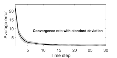
(a) Convergence of the average error

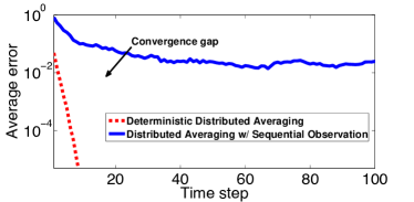
(b) Comparison with deterministic Distributed Averaging

Figure 1: Performance evaluation over a static undirected graph

It can be readily seen that our algorithm converges nicely with bounded variance. Moreover, comparing its convergence with that of the deterministic distributed averaging algorithm, where true beliefs are revealed to each agent at the initial time step, we see a clear (order-wise) gap between these two scenarios, which is primarily due to the sequential arriving nature of the data in our sequential data arriving setting (notice that in Fig. 1b we have changed the y-axis to log scale). This also validates the proved ${O}(1/t)$ convergence rate of the algorithm, which is order-wise slower than the deterministic scenario (which is exponentially fast).

We then investigate the convergence performance over a time-varying undirected graph. Following [29], we generate random probabilistic dynamic-graphs on the basis of a connected union graph. In particular, given a union graph $({\mathcal{N}},{\mathcal{E}})$, the agents $i$ and $j$ with $(i,j)\in{\mathcal{E}}$ are connected with probability $p$, generating a time-varying $\mathbb{N}(t)$. We make sure that the generated graph is connected. Note that such time-varying graphs satisfy both Assumptions 2 and 6. The Metropolis weights are then calculated over this $\mathbb{N}(t)$ at each time $t$. As shown in Fig. 2, a higher value of $p$ leads to a faster convergence rate as expected. Moreover, a smaller variance is incurred when the graph has less variability over time. In any case, the polynomial convergence rate shown in Theorem 1 is corroborated.

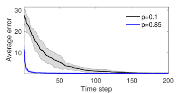
(a)

Figure 2: Performance evaluation over a time-varying undirected graph

6.2 Directed Graphs

We next investigate the convergence performance over directed graphs. To generate random directed graphs, we first generate undirected RGGs and then randomly delete some of the unidirectional edges between agents. With a fixed union graph, a time-varying graph is generated in the same way as in Section 6.1. Thus, the graphs satisfy Assumption 3. We have tested the update (6) for both static and time-varying graphs. It can be seen in Fig. 3 that the network-wide belief averaging is successfully achieved at polynomial rate, which corroborates the theoretical results in Theorem 2. Similarly, a higher value of $p$ results in a faster convergence rate and a smaller variance.

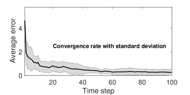
(a) Convergence of the average error over a static graph

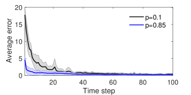
(b) Convergence of the average error over a time-varying graph

Figure 3: Performance evaluation over a directed graph

6.3 Quantization

In addition, we also study the effects of the two sources of quantization considered in Section 4. To satisfy conditions A.1) and A.2) in Assumption 4, we adopt a modified Metropolis weight as in [25]. Specifically, we let

$$w_{ij}(t) =\frac{1}{C(1+\max\{n_{i}(t),n_{j}(t)\})}~{},\;\;(i,j)\in\mathbb{N}(t)~{},$$ (34)

with $C>1$ and $w_{ii}(t)$ selected such that $\sum_{j=1}^{n}w_{ij}(t)=1$. Moreover, we choose the communication quantizer ${\mathcal{Q}}$ to be the truncation operator, and the precision $\Delta$ to be $0.1$. We first consider the case when the local belief $\bar{x}_{t}\notin{\mathcal{B}}$ for any $i\in{\mathcal{N}}$. It is demonstrated in Fig. 4 that over a static undirected graph, the average error $e(t)$ indeed converges in around $130$ iterations under the quantization we consider. In contrast to the results without quantization, however, the convergence of the error $e(t)$ is stalled at somewhere above zero (note that we have log scale y-axis in Fig. 4a). In fact, as shown in Fig. 4b, the local state $y_{i}(t)$ converges to the neighborhood of the average belief at a very fast rate. In the middle of convergence, oscillation of the states is observed, which is similar to the cyclic behavior as reported in [25]. Due to the stochastic nature of the sequential data, the oscillation may not be exact cyclic. Eventually, the local state values converge to the quantized consensus that deviates from the actual average belief by less than $1$. More examples have been observed to have similar convergence results as shown in Fig. 4, which corroborate the convergence results in Proposition 1.

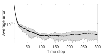
(a) Convergence of the average error

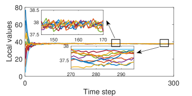
(b) Convergence of the local state $y_{i}(t)$

Figure 4: Performance evaluation under quantization over a static graph. In (b), each curve corresponds to the evolution of local state $y_{i}(t)$ at each agent.

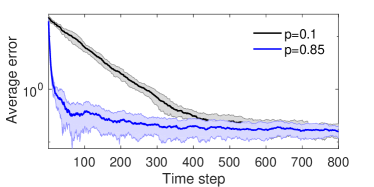
(a) Convergence of the average error

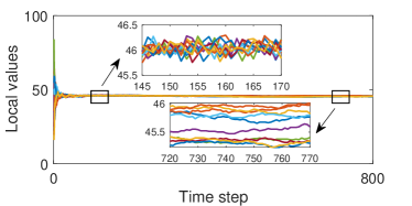
(b) Convergence of the local state $y_{i}(t)$ with $p=0.85$

Figure 5: Performance evaluation under quantization over a time-varying graph. In (b), each curve corresponds to the evolution of local state $y_{i}(t)$ at each agent.

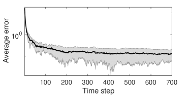
(a) Convergence of the average error

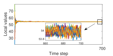
(b) Convergence of the local state $y_{i}(t)$

Figure 6: Performance evaluation under quantization when $\bar{x}_{i}\in{\mathcal{B}}$ for all $i\in{\mathcal{N}}$. In (b), each curve corresponds to the evolution of local state $y_{i}(t)$ at each agent.

Likewise, as shown in Fig. 5a, over a time-varying graph, the average error $e(t)$ converges (in around $300$ and $600$ iterations for $p=0.85$ and $p=0.1$, respectively), at a relatively slower rate than the case with a static graph. Moreover, the error $e(t)$ still fails to converge to exactly zero due to the quantization effects. Furthermore, the convergence behavior of the local states $y_{i}(t)$ in Fig. 5b resembles what is shown in Fig. 4b, while it takes longer time to converge to quantized consensus. Additionally, we are also interested in the convergence performance when some local beliefs $\bar{x}_{i}$ are inside the belief set ${\mathcal{B}}$. We thus specifically round the random beliefs $\bar{x}_{i}$ to the set ${\mathcal{B}}$ by finding the value in ${\mathcal{B}}$ that is closest to $\bar{x}_{i}$ in magnitude. Fig. 6a illustrates that the local states also fail to reach exact consensus to the average belief. Interestingly, the states here do not achieve the quantized consensus as in Fig. 4b and Fig.5b, while keep oscillating (though not exact cycling) around the neighborhood of the consensual belief. This somehow reflects the difficulty we encountered in theoretical analysis, that the difference of the running average with limited precision will randomly take values from $\Delta$, $-\Delta$, or $0$ (see Remark 2). The random error $\Delta\tilde{z}_{i}(t)$ does not accumulate over time and the size of the neighborhood is bounded to be within $1$.

6.4 Convergence Speed

We also numerically investigate how the convergence speed is influenced by the quantization effects. As shown in Fig. 7, we compare the convergence of the average errors under various levels of quantization. Note that $\Delta=0$ represents the case where only communication quantization exists and the division operation leads to no precision errors. As expected, a higher level of quantization leads to a slower convergence rate and a larger steady-state error. Surprisingly, however, the convergence rate is insensitive to either sources of quantizations. This implies that $O(1/t)$ seems to be an inherent convergence rate in the distributed averaging problem using sequential data. Thus, we conjecture that the rate to reach consensus under quantization is still in the order of $O(1/t)$, whose proof is left for future work.

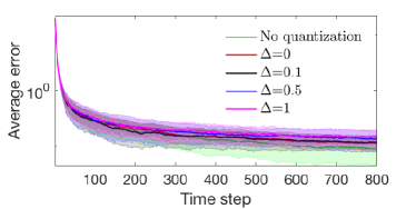
(a)

Figure 7: Performance evaluation under various levels of quantizations.

7 Conclusion

In this paper, we have studied distributed learning of average belief over networks with sequential observations, where in contrast to the conventional distributed averaging problem setting, each agent’s local belief is not available immediately and can only be learned through its own observations. Two distributed algorithms have been introduced for solving the problem over time-varying undirected and directed graphs, and their polynomial convergence rates have been established. We have also modified the algorithm for the practical case in which both quantized communication and limited precision of division operation occur. Numerical results have been provided to corroborate our theoretical findings.

For future work, we plan to investigate other important aspects of the proposed scheme for distributed learning of average belief with sequential data, e.g., the case under malicious data attack or with privacy requirement among agents. It is also interesting to connect the proposed scheme with other distributed and multi-agent learning algorithms [36, 22, 37, 38, 39].

The work of K. Zhang and T. Başar was supported in part by Office of Naval Research (ONR) MURI Grant N00014-16-1-2710, and in part by US Army Research Office (ARO) Grant W911NF-16-1-0485. The work of M. Liu is partially supported by the NSF under grants ECCS 1446521, CNS-1646019, and CNS-1739517. The authors also thank Zhuoran Yang from Princeton University for the helpful discussion that improves the final version of the paper.

References

- [1] Y. Liu, J. Liu, T. Başar, and M. Liu. Distributed belief averaging using sequential observations. In Proceedings of the 2017 American Control Conference, pages 680–685, 2017.
- [2] A. Jadbabaie, J. Lin, and A. S. Morse. Coordination of groups of mobile autonomous agents using nearest neighbor rules. IEEE Transactions on Automatic Control, 48(6):988–1001, 2003.
- [3] J. Cortés, S. Martínez, T. Karataş, and F. Bullo. Coverage control for mobile sensing networks. IEEE Transactions on Robotics and Automation, 20(2):243–255, 2004.
- [4] K. Zhang, W. Shi, H. Zhu, E. Dall’Anese, and T. Başar. Dynamic power distribution system management with a locally connected communication network. IEEE Journal of Selected Topics in Signal Processing, 12(4):673–687, 2018.
- [5] K. Zhang, L. Lu, C. Lei, H. Zhu, and Y. Ouyang. Dynamic operations and pricing of electric unmanned aerial vehicle systems and power networks. Transportation Research Part C: Emerging Technologies, 92:472–485, 2018.
- [6] L. Krick, M. E. Broucke, and B. A. Francis. Stabilisation of infinitesimally rigid formations of multi-robot networks. International Journal of Control, 82(3):423–439, 2009.
- [7] S. Kar, J. M. Moura, and K. Ramanan. Distributed parameter estimation in sensor networks: Nonlinear observation models and imperfect communication. IEEE Transactions on Information Theory, 58(6):3575–3605, 2012.
- [8] J. Liu, N. Hassanpour, S. Tatikonda, and A. S. Morse. Dynamic threshold models of collective action in social networks. In Proceedings of the 51st IEEE Conference on Decision and Control, pages 3991–3996, 2012.
- [9] T. Chen, S. Barbarossa, X. Wang, G. B. Giannakis, and Z. Zhang. Learning and management for Internet-of-Things: Accounting for adaptivity and scalability. Proc. of the IEEE, November 2018.
- [10] K. Zhang, W. Shi, H. Zhu, and T. Başar. Distributed equilibrium-learning for power network voltage control with a locally connected communication network. In IEEE Annual American Control Conference, pages 3092–3097. IEEE, 2018.
- [11] A. Kashyap, T. Başar, and R. Srikant. Quantized consensus. Automatica, 43(7):1192–1203, 2007.
- [12] L. Xiao and S. Boyd. Fast linear iterations for distributed averaging. Systems and Control Letters, 53(1):65–78, 2004.
- [13] L. Xiao, S. Boyd, and S. Lall. A scheme for robust distributed sensor fusion based on average consensus. In Proceedings of the 4th International Conference on Information Processing in Sensor Networks, pages 63–70, 2005.
- [14] S. Boyd, A. Ghosh, B. Prabhakar, and D. Shah. Randomized gossip algorithms. IEEE Transactions on Information Theory, 52(6):2508–2530, 2006.
- [15] J. Liu, S. Mou, A. S. Morse, B. D. O. Anderson, and C. Yu. Deterministic gossiping. Proceedings of the IEEE, 99(9):1505–1524, 2011.
- [16] D. Kempe, A. Dobra, and J. Gehrke. Gossip-based computation of aggregate information. In Proceedings of the 44th Annual IEEE Symposium on Foundations of Computer Science, pages 482–491, 2003.
- [17] F. Bénézit, V. Blondel, P. Thiran, J. N. Tsitsiklis, and M. Vetterli. Weighted gossip: Distributed averaging using non-doubly stochastic matrices. In Proceedings of the 2010 IEEE International Symposium on Information Theory, pages 1753–1757, 2010.
- [18] A. D. Domínguez-García, S. T. Cady, and C. N. Hadjicostis. Decentralized optimal dispatch of distributed energy resources. In Proceedings of the 51st IEEE Conference on Decision and Control, pages 3688–3693, 2012.
- [19] J. Liu and A. S. Morse. Asynchronous distributed averaging using double linear iterations. In Proceedings of the 2012 American Control Conference, pages 6620–6625, 2012.
- [20] M. Huang and J. H. Manton. Coordination and consensus of networked agents with noisy measurements: Stochastic algorithms and asymptotic behavior. SIAM Journal on Control and Optimization, 48(1):134–161, 2009.
- [21] S. Kar and J. M. Moura. Consensus+innovations distributed inference over networks: Cooperation and sensing in networked systems. IEEE Signal Processing Magazine, 30(3):99–109, 2013.
- [22] M. A. Rahimian and A. Jadbabaie. Distributed estimation and learning over heterogeneous networks. In Communication, Control, and Computing (Allerton), 2016 54th Annual Allerton Conference on, pages 1314–1321, 2016.
- [23] A. Nedić, A. Olshevsky, A. Ozdaglar, and J. N. Tsitsiklis. On distributed averaging algorithms and quantization effects. IEEE Transactions on Automatic Control, 54(11):2506–2517, 2009.
- [24] R. Carli, F. Fagnani, P. Frasca, and S. Zampieri. Gossip consensus algorithms via quantized communication. Automatica, 46(1):70–80, 2010.
- [25] M. El Chamie, J. Liu, and T. Başar. Design and analysis of distributed averaging with quantized communication. IEEE Transactions on Automatic Control, 61(12):3870–3884, 2016.
- [26] K. Cai and H. Ishii. Quantized consensus and averaging on gossip digraphs. IEEE Transactions on Automatic Control, 56(9):2087–2100, 2011.
- [27] T. Başar, S. R. Etesami, and A. Olshevsky. Fast convergence of quantized consensus using Metropolis chains. In Proceedings of the 53rd IEEE Conference on Decision and Control, pages 1330–1334. IEEE, 2014.
- [28] R. Durrett. Probability: Theory and Examples. Cambridge University Press, 2010.
- [29] M. El Chamie, J. Liu, T. Başar, and B. Açıkmeşe. Distributed averaging with quantized communication over dynamic graphs. In Proceedings of the 55th IEEE Conference on Decision and Control, pages 4827–4832. IEEE, 2016.
- [30] J. Lavaei and R. M. Murray. Quantized consensus by means of gossip algorithm. IEEE Transactions on Automatic Control, 57(1):19–32, 2012.
- [31] S. Patterson, B. Bamieh, and A. El Abbadi. Convergence rates of distributed average consensus with stochastic link failures. IEEE Transactions on Automatic Control, 55(4):880–892, 2010.
- [32] J. Liu, A. S. Morse, A. Nedić, and T. Başar. Internal stability of linear consensus processes. In Proceedings of the 53rd IEEE Conference on Decision and Control, pages 922–927, 2014.
- [33] E. Seneta. Non-negative Matrices and Markov Chains. Sringer, 2006.
- [34] J. Liu, T. Başar, and A. Nedić. Input-output stability of linear consensus processes. In Proceedings of the 55th IEEE Conference on Decision and Control, pages 6978–6983, 2016.
- [35] A. Nedić and A. Olshevsky. Distributed optimization over time-varying directed graphs. IEEE Transactions on Automatic Control, 60(3):601–615, 2015.
- [36] O. Shamir. Fundamental limits of online and distributed algorithms for statistical learning and estimation. In Advances in Neural Information Processing Systems, pages 163–171, 2014.
- [37] W. Zhang, P. Zhao, W. Zhu, S. C. Hoi, and T. Zhang. Projection-free distributed online learning in networks. In International Conference on Machine Learning, pages 4054–4062, 2017.
- [38] K. Zhang, Z. Yang, H. Liu, T. Zhang, and T. Başar. Fully decentralized multi-agent reinforcement learning with networked agents. In International Conference on Machine Learning, pages 5867–5876, 2018.
- [39] K. Zhang, Z. Yang, and T. Başar. Networked multi-agent reinforcement learning in continuous spaces. In Proceedings of the 57rd IEEE Conference on Decision and Control, 2018.