Correlation effects in spin models in the presence of a spin bath

Álvaro Gómez-León1, Tim Cox2 and Philip Stamp2 1Instituto de Ciencia de Materiales, CSIC, Cantoblanco, Madrid E-28049, Spain 2Department of Physics and Astronomy, University of British Columbia, 6224 Agricultural Road, Vancouver, British Columbia, V6T 1Z1, Canada
(March 15, 2024)
Abstract

We analyze the effect of a bath of spins interacting with a spin system in terms of the equation of motion technique. We show that this formalism can be used with general spin systems and baths, and discuss the concrete case of a Quantum Ising model longitudinally coupled to the bath. We show how the uncorrelated solutions change when spin-spin correlations are included, the properties of the quasiparticle excitations and the effect of internal dynamics in the spin bath.

I Introduction

Spins systems are among the most studied models in physics, but their properties are also closely related with systems in many other fields of science VoterModel ; Biophysics ; BirdNavigation . These models are interesting because they display many emergent phenomena due to collective effects, and in addition, because of their relevance in the development of quantum computersQAnnealing . Most works on spin models mainly consider closed systems and study the equilibrium phase diagram, the critical exponents, and more recently, also the quench dynamicsQuenchDynamics-PhaseTrans ; sachdev_2011 . Less it is known about these models in the presence of environments, specially for those described by a collection of localized modes. These are known to produce radically different effects than the usual oscillator bath in certain regimes LiHoFPhaseTransition ; HyperfineLiHoF ; Theory-SpinBath . As the coupling to localized spin environments is generally not weak111Typically oscillator bath couplings scale as 1/N1𝑁1/\sqrt{N} due to their delocalized nature, being N𝑁N the number of modes. Therefore perturbative calculations can, in most cases, capture the main properties., the calculations are generally non-perturbative and must be done carefully, which implies that in the case of quantum models, the effect of correlations can become quite important.

For practical purposes, the study of spin models has recently become more important due to the development of the first quantum simulators and quantum computers D-wave ; Google-QC ; IBM . In this case, environments are ubiquitous and its interaction with the quantum computer during the computation time needs to be properly understood – e.g., the fate of the quantum critical point (QCP) during the quantum annealing process, in the presence of an environment. In the case of quantum computers made of flux qubits, spin environments can be produced by paramagnetic impurities and nuclear isotopes in the substrate, and even if they weakly couple, their effect in the dynamics can be non-trivial SQUID-dyn . Also it has been shown that for superconducting qubits dielectric loss can dominate, and it is produced by effective two level systems MartinisDecoherenceSquid .

To understand the physical effect of spin bath environments we study a spin model coupled to a set of localized spins. We use the equation of motion (EOM) technique for the Green’s functions, and a decoupling scheme based on a hierarchical expansion in terms of correlations. This approach transforms the EOM into a Dyson’s equation for the Green’s function, with explicit non-perturbative expressions for the self-energy, which include a full frequency and momentum dependence. Hence it can also be used to study quantum dynamics of excited states, as already shown in AnalyticalDecoherence . The lowest order solution agrees with mean-field (MF) treatments and can explain some general features of the effect of a baths of spins, as the solutions are solely characterized by the connectivity between Ising spins and bath spins (i.e., the three different coordination numbers that one can define for this model). Higher order corrections depend on the specific details of the bath, however, we numerically solve the self-consistent equations for some specific cases and demonstrate that quantum correlations tend to suppress the effect of the bath of spins, with respect to the MF calculations.

II Model and method

We consider a model with a central system and a bath. The central system is made of a set of interacting spins coupled to an external field B→→𝐡\vec{B}. Similarly, the bath is made of a set of spins as well, but we assume that these are non-interacting, although they can be affected by an external field Ξ”β†’β†’Ξ”\vec{\Delta}222Interactions between bath spins can be easily introduced, but it is known that large interactions would make the environment behave as an effective oscillator bath, as the modes would not be localized anymore.. The total Hamiltonian is H=HS+HB𝐻subscript𝐻𝑆subscript𝐻𝐡H=H_{S}+H_{B}, where HSsubscript𝐻𝑆H_{S} and HBsubscript𝐻𝐡H_{B} are given by (Greek indices specify the direction of the spin vector and latin indices label the different sites):

HSsubscript𝐻𝑆\displaystyle H_{S} =\displaystyle= βˆ’βˆ‘ΞΌ,iBμ​SiΞΌβˆ’βˆ‘ΞΌβˆ‘i,j>iVi,jμ​Siμ​SjΞΌsubscriptπœ‡π‘–subscriptπ΅πœ‡superscriptsubscriptπ‘†π‘–πœ‡subscriptπœ‡subscript𝑖𝑗𝑖superscriptsubscriptπ‘‰π‘–π‘—πœ‡superscriptsubscriptπ‘†π‘–πœ‡superscriptsubscriptπ‘†π‘—πœ‡\displaystyle-\sum_{\mu,i}B_{\mu}S_{i}^{\mu}-\sum_{\mu}\sum_{i,j>i}V_{i,j}^{\mu}S_{i}^{\mu}S_{j}^{\mu} (1)
HBsubscript𝐻𝐡\displaystyle H_{B} =\displaystyle= βˆ’βˆ‘ΞΌ,lΔμ​IlΞΌ+βˆ‘ΞΌβˆ‘i,lAi,lμ​Siμ​IlΞΌsubscriptπœ‡π‘™subscriptΞ”πœ‡superscriptsubscriptπΌπ‘™πœ‡subscriptπœ‡subscript𝑖𝑙superscriptsubscriptπ΄π‘–π‘™πœ‡superscriptsubscriptπ‘†π‘–πœ‡superscriptsubscriptπΌπ‘™πœ‡\displaystyle-\sum_{\mu,l}\Delta_{\mu}I_{l}^{\mu}+\sum_{\mu}\sum_{i,l}A_{i,l}^{\mu}S_{i}^{\mu}I_{l}^{\mu} (2)

HSsubscript𝐻𝑆H_{S} corresponds to a general spin model coupled to an external field B→→𝐡\vec{B} and with arbitrary interaction Vi,jΞΌsuperscriptsubscriptπ‘‰π‘–π‘—πœ‡V_{i,j}^{\mu}, while HBsubscript𝐻𝐡H_{B} corresponds to the bath Hamiltonian which couples to a field Ξ”β†’β†’Ξ”\vec{\Delta} and interacts with the central system via Ai,lΞΌsuperscriptsubscriptπ΄π‘–π‘™πœ‡A_{i,l}^{\mu}. To study the properties of the system we define the next double-time Green’s functions Zubarev :

Gn,mΞ±,β​(t,tβ€²)superscriptsubscriptπΊπ‘›π‘šπ›Όπ›½π‘‘superscript𝑑′\displaystyle G_{n,m}^{\alpha,\beta}\left(t,t^{\prime}\right) =\displaystyle= βˆ’iβ€‹βŸ¨Snα​(t);Omβ​(tβ€²)βŸ©π‘–superscriptsubscript𝑆𝑛𝛼𝑑superscriptsubscriptπ‘‚π‘šπ›½superscript𝑑′\displaystyle-i\langle S_{n}^{\alpha}\left(t\right);O_{m}^{\beta}\left(t^{\prime}\right)\rangle (3)
Yn,mΞ±,β​(t,tβ€²)superscriptsubscriptπ‘Œπ‘›π‘šπ›Όπ›½π‘‘superscript𝑑′\displaystyle Y_{n,m}^{\alpha,\beta}\left(t,t^{\prime}\right) =\displaystyle= βˆ’iβ€‹βŸ¨Inα​(t);Omβ​(tβ€²)βŸ©π‘–superscriptsubscript𝐼𝑛𝛼𝑑superscriptsubscriptπ‘‚π‘šπ›½superscript𝑑′\displaystyle-i\langle I_{n}^{\alpha}\left(t\right);O_{m}^{\beta}\left(t^{\prime}\right)\rangle (4)

where ; indicates that the Green’s functions may be a time ordered, retarded or advanced. Also OmΞ²superscriptsubscriptπ‘‚π‘šπ›½O_{m}^{\beta} is some general spin operator at site mπ‘šm (i.e., it can represent a system or a bath spin). The equation of motion for the Green’s function is:

iβ€‹βˆ‚tGn,mΞ±,β𝑖subscript𝑑superscriptsubscriptπΊπ‘›π‘šπ›Όπ›½\displaystyle i\partial_{t}G_{n,m}^{\alpha,\beta} =\displaystyle= δ​(tβˆ’tβ€²)β€‹βŸ¨[SnΞ±,OmΞ²]±⟩+i​ϡμ​α​ρ​Bμ​Gn,mρ,β𝛿𝑑superscript𝑑′delimited-⟨⟩subscriptsuperscriptsubscript𝑆𝑛𝛼superscriptsubscriptπ‘‚π‘šπ›½plus-or-minus𝑖subscriptitalic-Ο΅πœ‡π›ΌπœŒsubscriptπ΅πœ‡superscriptsubscriptπΊπ‘›π‘šπœŒπ›½\displaystyle\delta\left(t-t^{\prime}\right)\langle\left[S_{n}^{\alpha},O_{m}^{\beta}\right]_{\pm}\rangle+i\epsilon_{\mu\alpha\rho}B_{\mu}G_{n,m}^{\rho,\beta}
+i​ϡμ​α​ρ​(βˆ‘iβ‰ nVi,nμ​Gi​n,mμ​ρ,Ξ²βˆ’βˆ‘lAn,lμ​Yl​n,mμ​ρ,Ξ²)𝑖subscriptitalic-Ο΅πœ‡π›ΌπœŒsubscript𝑖𝑛superscriptsubscriptπ‘‰π‘–π‘›πœ‡superscriptsubscriptπΊπ‘–π‘›π‘šπœ‡πœŒπ›½subscript𝑙superscriptsubscriptπ΄π‘›π‘™πœ‡superscriptsubscriptπ‘Œπ‘™π‘›π‘šπœ‡πœŒπ›½\displaystyle+i\epsilon_{\mu\alpha\rho}\left(\sum_{i\neq n}V_{i,n}^{\mu}G_{in,m}^{\mu\rho,\beta}-\sum_{l}A_{n,l}^{\mu}Y_{ln,m}^{\mu\rho,\beta}\right)

where […]Β±subscriptdelimited-[]…plus-or-minus\left[\ldots\right]_{\pm} refers to anti-commutator or commutator, respectivelyFermionic-GF ; SCHREIBER197927 (i.e., to a fermionic or bosonic Green’s function). We have defined the three-spin correlators Gi​n,mμ​ρ,β​(t,tβ€²)=βˆ’iβ€‹βŸ¨Siμ​Snρ;Omβ⟩superscriptsubscriptπΊπ‘–π‘›π‘šπœ‡πœŒπ›½π‘‘superscript𝑑′𝑖superscriptsubscriptπ‘†π‘–πœ‡superscriptsubscriptπ‘†π‘›πœŒsuperscriptsubscriptπ‘‚π‘šπ›½G_{in,m}^{\mu\rho,\beta}\left(t,t^{\prime}\right)=-i\langle S_{i}^{\mu}S_{n}^{\rho};O_{m}^{\beta}\rangle and Yl​n,mν​ρ,β​(t,tβ€²)=βˆ’iβ€‹βŸ¨Ilν​Snρ;Omβ⟩superscriptsubscriptπ‘Œπ‘™π‘›π‘šπœˆπœŒπ›½π‘‘superscript𝑑′𝑖superscriptsubscriptπΌπ‘™πœˆsuperscriptsubscriptπ‘†π‘›πœŒsuperscriptsubscriptπ‘‚π‘šπ›½Y_{ln,m}^{\nu\rho,\beta}\left(t,t^{\prime}\right)=-i\langle I_{l}^{\nu}S_{n}^{\rho};O_{m}^{\beta}\rangle.

An important feature of many-body systems is the hierarchical structure of the EOM, where interaction terms produce higher-order Green’s functions. To deal with this hierarchy, one needs to devise a method to decouple the infinite set of equations into smaller blocks, which correctly captures the regime of interest. For that purpose we separate the Green’s functions into their uncorrelated and correlated parts: Gi​n,mμ​ρ,Ξ²=⟨SiΞΌβŸ©β€‹Gn,mρ,Ξ²+⟨SnΟβŸ©β€‹Gi,mΞΌ,Ξ²+𝒒i​n,mμ​ρ,Ξ²superscriptsubscriptπΊπ‘–π‘›π‘šπœ‡πœŒπ›½delimited-⟨⟩superscriptsubscriptπ‘†π‘–πœ‡superscriptsubscriptπΊπ‘›π‘šπœŒπ›½delimited-⟨⟩superscriptsubscriptπ‘†π‘›πœŒsuperscriptsubscriptπΊπ‘–π‘šπœ‡π›½superscriptsubscriptπ’’π‘–π‘›π‘šπœ‡πœŒπ›½G_{in,m}^{\mu\rho,\beta}=\langle S_{i}^{\mu}\rangle G_{n,m}^{\rho,\beta}+\langle S_{n}^{\rho}\rangle G_{i,m}^{\mu,\beta}+\mathcal{G}_{in,m}^{\mu\rho,\beta} (we will use calligraphic letters to denote the correlated parts). This separation is completely general and just transforms the initial EOM for the two-point function in two coupled equations, one for the two-point functions and one for the correlated parts. Physically, the terms ⟨SiΞΌβŸ©β€‹Gn,mρ,Ξ²+⟨SnΟβŸ©β€‹Gi,mΞΌ,Ξ²delimited-⟨⟩superscriptsubscriptπ‘†π‘–πœ‡superscriptsubscriptπΊπ‘›π‘šπœŒπ›½delimited-⟨⟩superscriptsubscriptπ‘†π‘›πœŒsuperscriptsubscriptπΊπ‘–π‘šπœ‡π›½\langle S_{i}^{\mu}\rangle G_{n,m}^{\rho,\beta}+\langle S_{n}^{\rho}\rangle G_{i,m}^{\mu,\beta} are similar to the Hartree and Fock contributions. They capture the average effect of all the other spins on the two-point function, while the correlated part 𝒒i​n,mμ​ρ,Ξ²superscriptsubscriptπ’’π‘–π‘›π‘šπœ‡πœŒπ›½\mathcal{G}_{in,m}^{\mu\rho,\beta} contains the corrections due to correlations with additional spins.

Our approximation to close the system of equations will assume that correlated parts scale in some particular way with the parameters of the system, such that they can be neglected when they are small enoughHierarchyCorr-Majorana ; HIerarchy-Topology . We will organize terms in inverse powers of the coordination number Z𝑍Z, where Z𝑍Z generally denotes any coordination number required to describe the model (for the Ising model just one coordination number is required, while for the examples below we show that three different coordination numbers are needed. In this case the smallest coordination number will dominate the scaling). Doing this, it is possible to systematically include higher order corrections by simply adding higher order correlated parts.

It must be mentioned that the scaling of correlations converges more slowly in 1D (it goes as ∼Zβˆ’1similar-toabsentsuperscript𝑍1\sim Z^{-1}, with Z=2𝑍2Z=2). However, it is still an interesting case, because in low dimensional systems quantum corrections are usually enhanced. This facilitates the study of quantum corrections due to the spin bath, and for this reason we will consider the 1D case for the numerical results. However one must keep in mind that the equations are general for arbitrary dimension. Furthermore, we will show that including the correlated parts in the equation of motion, allows to recover the exact quantum critical point in absence of the spin bath, thus providing a good benchmark for our results. For accurate results in low dimensional cases, the present technique could also be combined with different fermionization or bosonization techniquessachdev_2011 , and straightforwardly applying the same Green’s function analysis.

Let us apply this decoupling scheme to Eq.II and Fourier transform to frequency domain. One finds:

ω​Gn,mΞ±,Ξ²πœ”superscriptsubscriptπΊπ‘›π‘šπ›Όπ›½\displaystyle\omega G_{n,m}^{\alpha,\beta} =\displaystyle= ⟨[SnΞ±,OmΞ²]±⟩+iβ€‹βˆ‘ΞΌΟ΅ΞΌβ€‹Ξ±β€‹Οβ€‹(BΞΌ+βˆ‘iβ‰ nVi,nΞΌβ€‹βŸ¨SiΞΌβŸ©βˆ’βˆ‘lAn,lΞΌβ€‹βŸ¨Ilμ⟩)​Gn,mρ,Ξ²delimited-⟨⟩subscriptsuperscriptsubscript𝑆𝑛𝛼superscriptsubscriptπ‘‚π‘šπ›½plus-or-minus𝑖subscriptπœ‡subscriptitalic-Ο΅πœ‡π›ΌπœŒsubscriptπ΅πœ‡subscript𝑖𝑛superscriptsubscriptπ‘‰π‘–π‘›πœ‡delimited-⟨⟩superscriptsubscriptπ‘†π‘–πœ‡subscript𝑙superscriptsubscriptπ΄π‘›π‘™πœ‡delimited-⟨⟩superscriptsubscriptπΌπ‘™πœ‡superscriptsubscriptπΊπ‘›π‘šπœŒπ›½\displaystyle\langle\left[S_{n}^{\alpha},O_{m}^{\beta}\right]_{\pm}\rangle+i\sum_{\mu}\epsilon_{\mu\alpha\rho}\left(B_{\mu}+\sum_{i\neq n}V_{i,n}^{\mu}\langle S_{i}^{\mu}\rangle-\sum_{l}A_{n,l}^{\mu}\langle I_{l}^{\mu}\rangle\right)G_{n,m}^{\rho,\beta}
+iβ€‹βˆ‘ΞΌΟ΅ΞΌβ€‹Ξ±β€‹Οβ€‹(βˆ‘iβ‰ nVi,nμ​(⟨SnΟβŸ©β€‹Gi,mΞΌ,Ξ²+𝒒i​n,mμ​ρ,Ξ²)βˆ’βˆ‘lAn,lμ​(⟨SnΟβŸ©β€‹Yl,mΞΌ,Ξ²+𝒴l​n,mμ​ρ,Ξ²))𝑖subscriptπœ‡subscriptitalic-Ο΅πœ‡π›ΌπœŒsubscript𝑖𝑛superscriptsubscriptπ‘‰π‘–π‘›πœ‡delimited-⟨⟩superscriptsubscriptπ‘†π‘›πœŒsuperscriptsubscriptπΊπ‘–π‘šπœ‡π›½superscriptsubscriptπ’’π‘–π‘›π‘šπœ‡πœŒπ›½subscript𝑙superscriptsubscriptπ΄π‘›π‘™πœ‡delimited-⟨⟩superscriptsubscriptπ‘†π‘›πœŒsuperscriptsubscriptπ‘Œπ‘™π‘šπœ‡π›½superscriptsubscriptπ’΄π‘™π‘›π‘šπœ‡πœŒπ›½\displaystyle+i\sum_{\mu}\epsilon_{\mu\alpha\rho}\left(\sum_{i\neq n}V_{i,n}^{\mu}\left(\langle S_{n}^{\rho}\rangle G_{i,m}^{\mu,\beta}+\mathcal{G}_{in,m}^{\mu\rho,\beta}\right)-\sum_{l}A_{n,l}^{\mu}\left(\langle S_{n}^{\rho}\rangle Y_{l,m}^{\mu,\beta}+\mathcal{Y}_{ln,m}^{\mu\rho,\beta}\right)\right)

The first line corresponds to the uncorrelated contribution, while the second line corresponds to the contribution from correlations between spins. Notice the appearance of the Green’s function Yl,mΞΌ,Ξ²=βˆ’iβ€‹βŸ¨IlΞΌ;Omβ⟩superscriptsubscriptπ‘Œπ‘™π‘šπœ‡π›½π‘–superscriptsubscriptπΌπ‘™πœ‡superscriptsubscriptπ‘‚π‘šπ›½Y_{l,m}^{\mu,\beta}=-i\langle I_{l}^{\mu};O_{m}^{\beta}\rangle, which couples the equation of motion for the Ising spins with the one for the bath spins:

ω​Yn,mΞ±,Ξ²πœ”superscriptsubscriptπ‘Œπ‘›π‘šπ›Όπ›½\displaystyle\omega Y_{n,m}^{\alpha,\beta} =\displaystyle= ⟨[InΞ±,OmΞ²]±⟩+iβ€‹βˆ‘ΞΌΟ΅ΞΌβ€‹Ξ±β€‹Οβ€‹(Ξ”ΞΌβˆ’βˆ‘iAi,nΞΌβ€‹βŸ¨Siμ⟩)​Yn,mρ,Ξ²delimited-⟨⟩subscriptsuperscriptsubscript𝐼𝑛𝛼superscriptsubscriptπ‘‚π‘šπ›½plus-or-minus𝑖subscriptπœ‡subscriptitalic-Ο΅πœ‡π›ΌπœŒsubscriptΞ”πœ‡subscript𝑖superscriptsubscriptπ΄π‘–π‘›πœ‡delimited-⟨⟩superscriptsubscriptπ‘†π‘–πœ‡superscriptsubscriptπ‘Œπ‘›π‘šπœŒπ›½\displaystyle\langle\left[I_{n}^{\alpha},O_{m}^{\beta}\right]_{\pm}\rangle+i\sum_{\mu}\epsilon_{\mu\alpha\rho}\left(\Delta_{\mu}-\sum_{i}A_{i,n}^{\mu}\langle S_{i}^{\mu}\rangle\right)Y_{n,m}^{\rho,\beta}
βˆ’iβ€‹βˆ‘ΞΌ,iϡμ​α​ρ​Ai,nμ​(⟨InΟβŸ©β€‹Gi,mΞΌ,Ξ²+𝒴n​i,mρ​μ,Ξ²)𝑖subscriptπœ‡π‘–subscriptitalic-Ο΅πœ‡π›ΌπœŒsuperscriptsubscriptπ΄π‘–π‘›πœ‡delimited-⟨⟩superscriptsubscriptπΌπ‘›πœŒsuperscriptsubscriptπΊπ‘–π‘šπœ‡π›½superscriptsubscriptπ’΄π‘›π‘–π‘šπœŒπœ‡π›½\displaystyle-i\sum_{\mu,i}\epsilon_{\mu\alpha\rho}A_{i,n}^{\mu}\left(\langle I_{n}^{\rho}\rangle G_{i,m}^{\mu,\beta}+\mathcal{Y}_{ni,m}^{\rho\mu,\beta}\right)

Finally, one can write the equations in a more compact form using matrix notation:

(Ο‰βˆ’β„^)β‹…G^β‹…πœ”^ℍ^𝐺\displaystyle\left(\omega-\hat{\mathbb{H}}\right)\cdot\hat{G} =\displaystyle= Ο‡^Β±+V^⋅𝒒^superscript^πœ’plus-or-minusβ‹…^𝑉^𝒒\displaystyle\hat{\chi}^{\pm}+\hat{V}\cdot\hat{\mathcal{G}} (8)

where G^^𝐺\hat{G} is a vector containing all the system and bath two-point functions, Ο‡^Β±superscript^πœ’plus-or-minus\hat{\chi}^{\pm} contains the source terms coming from the commutators/anti-commutators, 𝒒^^𝒒\hat{\mathcal{G}} contains all extra contributions from correlations, V^^𝑉\hat{V} is the general interaction matrix for the correlated parts, and ℍ^^ℍ\hat{\mathbb{H}} is the effective Hamiltonian for the two-point Green’s functions. If the contribution from the correlated parts 𝒒^^𝒒\hat{\mathcal{G}} is small enough, the solution can be obtained by direct matrix inversion. This is a good approximation near fixed points of the RG flow, where solutions are approximately described by free spin Hamiltonians with renormalized parameters. Furthermore, if one defines g^=(Ο‰βˆ’β„^)βˆ’1^𝑔superscriptπœ”^ℍ1\hat{g}=\left(\omega-\hat{\mathbb{H}}\right)^{-1}, the previous equation resembles a Dyson’s equation, and from the correlated parts it can be shown that V^⋅𝒒^β‹…^𝑉^𝒒\hat{V}\cdot\hat{\mathcal{G}} can be written as Ξ£^​(Ο‰)β‹…G^β‹…^Ξ£πœ”^𝐺\hat{\Sigma}\left(\omega\right)\cdot\hat{G}, giving rise to the self-energy and the familiar Dyson’s equation.

G^=g^β‹…Ο‡^Β±+g^β‹…Ξ£^β‹…G^^𝐺⋅^𝑔superscript^πœ’plus-or-minusβ‹…^𝑔^Ξ£^𝐺\hat{G}=\hat{g}\cdot\hat{\chi}^{\pm}+\hat{g}\cdot\hat{\Sigma}\cdot\hat{G} (9)

III Uncorrelated solution

To close the system of equations one can neglect the correlated parts in Eq.8. Then the solution for the Green’s function is given by a matrix inversion. Eqs.II and II have two contributions from each interaction term, similar to the well known Hartree and Fock terms. If one ignores the Fock contribution, the coupling between Green’s functions at different sites vanishes and the equations are diagonal in real space. This is equivalent to derive an effective-medium Hamiltonian for each spin, where all correlations between sites are neglected. In this case one finds poles at Ο‰s​(n)=(βˆ‘Ξ±hsα​(n))2subscriptπœ”π‘ π‘›superscriptsubscript𝛼superscriptsubscriptβ„Žπ‘ π›Όπ‘›2\omega_{s}\left(n\right)=\sqrt{\left(\sum_{\alpha}h_{s}^{\alpha}\left(n\right)\right)^{2}} for the central system, and at Ο‰b​(n)=(βˆ‘Ξ±hbα​(n))2subscriptπœ”π‘π‘›superscriptsubscript𝛼superscriptsubscriptβ„Žπ‘π›Όπ‘›2\omega_{b}\left(n\right)=\sqrt{\left(\sum_{\alpha}h_{b}^{\alpha}\left(n\right)\right)^{2}} for the bath, where hsμ​(n)=BΞΌ+βˆ‘iβ‰ nVn,iμ​MiΞΌβˆ’βˆ‘lAn,lμ​mlΞΌsuperscriptsubscriptβ„Žπ‘ πœ‡π‘›subscriptπ΅πœ‡subscript𝑖𝑛superscriptsubscriptπ‘‰π‘›π‘–πœ‡superscriptsubscriptπ‘€π‘–πœ‡subscript𝑙superscriptsubscriptπ΄π‘›π‘™πœ‡superscriptsubscriptπ‘šπ‘™πœ‡h_{s}^{\mu}\left(n\right)=B_{\mu}+\sum_{i\neq n}V_{n,i}^{\mu}M_{i}^{\mu}-\sum_{l}A_{n,l}^{\mu}m_{l}^{\mu} and hbμ​(n)=Ξ”ΞΌβˆ’βˆ‘iAi,nμ​MiΞΌsuperscriptsubscriptβ„Žπ‘πœ‡π‘›subscriptΞ”πœ‡subscript𝑖superscriptsubscriptπ΄π‘–π‘›πœ‡superscriptsubscriptπ‘€π‘–πœ‡h_{b}^{\mu}\left(n\right)=\Delta_{\mu}-\sum_{i}A_{i,n}^{\mu}M_{i}^{\mu}. As the Green’s functions depend on the local magnetization MnΞ±=⟨Snα⟩superscriptsubscript𝑀𝑛𝛼delimited-⟨⟩superscriptsubscript𝑆𝑛𝛼M_{n}^{\alpha}=\langle S_{n}^{\alpha}\rangle and mnΞ±=⟨Inα⟩superscriptsubscriptπ‘šπ‘›π›Όdelimited-⟨⟩superscriptsubscript𝐼𝑛𝛼m_{n}^{\alpha}=\langle I_{n}^{\alpha}\rangle, they need to be determined self-consistency. Physically, this happens due to the non-linearities introduced by the interaction term. Defining the spectral function JΞ±,β​(Ο‰)=i​[gn,nΞ±,β​(Ο‰+i​ϡ)βˆ’gn,nΞ±,β​(Ο‰βˆ’i​ϡ)]​(eΟ‰TΒ±1)βˆ’1superscriptπ½π›Όπ›½πœ”π‘–delimited-[]superscriptsubscriptπ‘”π‘›π‘›π›Όπ›½πœ”π‘–italic-Ο΅superscriptsubscriptπ‘”π‘›π‘›π›Όπ›½πœ”π‘–italic-Ο΅superscriptplus-or-minussuperscriptπ‘’πœ”π‘‡11J^{\alpha,\beta}\left(\omega\right)=i\left[g_{n,n}^{\alpha,\beta}\left(\omega+i\epsilon\right)-g_{n,n}^{\alpha,\beta}\left(\omega-i\epsilon\right)\right]\left(e^{\frac{\omega}{T}}\pm 1\right)^{-1}, the self-consistency equations are obtained from the relation between the statistical average and the spectral function i2​ϡμ​ν​α​MnΞ±=∫JΞ½,μ​(Ο‰)​𝑑ω/2​π𝑖2subscriptitalic-Ο΅πœ‡πœˆπ›Όsuperscriptsubscript𝑀𝑛𝛼superscriptπ½πœˆπœ‡πœ”differential-dπœ”2πœ‹\frac{i}{2}\epsilon_{\mu\nu\alpha}M_{n}^{\alpha}=\int J^{\nu,\mu}\left(\omega\right)d\omega/2\pi Zubarev (the Β±plus-or-minus\pm sign corresponds to fermionic or bosonic Green’s function, respectively). The previous solution for the Green’s functions, in combination with the solutions of these non-linear equations characterizing the local magnetization MnΞ±superscriptsubscript𝑀𝑛𝛼M_{n}^{\alpha} and mlΞ±superscriptsubscriptπ‘šπ‘™π›Όm_{l}^{\alpha}, fully determine the properties of the system if correlations can be neglected. Furthermore, as in this uncorrelated case the Green’s functions display simple poles only, one can rewrite the integral over frequency as a sum over poles. Then the final form of the self-consistency equations is:

MnΞ±superscriptsubscript𝑀𝑛𝛼\displaystyle M_{n}^{\alpha} =\displaystyle= hsα​(n)2​ωs​(n)​tanh⁑(Ο‰s​(n)2​T)superscriptsubscriptβ„Žπ‘ π›Όπ‘›2subscriptπœ”π‘ π‘›subscriptπœ”π‘ π‘›2𝑇\displaystyle\frac{h_{s}^{\alpha}\left(n\right)}{2\omega_{s}\left(n\right)}\tanh\left(\frac{\omega_{s}\left(n\right)}{2T}\right) (10)
mnΞ±superscriptsubscriptπ‘šπ‘›π›Ό\displaystyle m_{n}^{\alpha} =\displaystyle= hbα​(n)2​ωb​(n)​tanh⁑(Ο‰b​(n)2​T)superscriptsubscriptβ„Žπ‘π›Όπ‘›2subscriptπœ”π‘π‘›subscriptπœ”π‘π‘›2𝑇\displaystyle\frac{h_{b}^{\alpha}\left(n\right)}{2\omega_{b}\left(n\right)}\tanh\left(\frac{\omega_{b}\left(n\right)}{2T}\right) (11)

This result has been particularized for spin 1/2, but larger spins can be studied similarly, as we discuss below for the specific case of the Quantum Ising model. This simple result is a good first estimate to see if the solutions are characterized by a magnetic texture. For example, it can capture the anti-ferromagnetic ordering for the case Vi,j<0subscript𝑉𝑖𝑗0V_{i,j}<0. With this information one can build more complete solutions, based on the symmetries of the ground states.

Quantum Ising model longitudinally coupled to the spin bath:

As a more specific case, let us consider the ferromagnetic Quantum Ising model, longitudinally coupled to a bath of spins (we set Vi,jx,y=0superscriptsubscript𝑉𝑖𝑗π‘₯𝑦0V_{i,j}^{x,y}=0, By,z=0subscript𝐡𝑦𝑧0B_{y,z}=0, Ai,lx,y=0superscriptsubscript𝐴𝑖𝑙π‘₯𝑦0A_{i,l}^{x,y}=0 and initially Ξ”β†’=0β†’Ξ”0\vec{\Delta}=0). In this case the poles for the central system are Ο‰s=B2+(V0​Mzβˆ’ZB​A​mz)2subscriptπœ”π‘ superscript𝐡2superscriptsubscript𝑉0subscript𝑀𝑧subscript𝑍𝐡𝐴subscriptπ‘šπ‘§2\omega_{s}=\sqrt{B^{2}+\left(V_{0}M_{z}-Z_{B}Am_{z}\right)^{2}}, while the ones for the bath are Ο‰b=ZB​S​A​Mzsubscriptπœ”π‘subscript𝑍𝐡𝑆𝐴subscript𝑀𝑧\omega_{b}=Z_{BS}AM_{z}. The self-consistency equations can be directly obtained from Eq.10 (to simplify notation we rename V0=ZS​Vsubscript𝑉0subscript𝑍𝑆𝑉V_{0}=Z_{S}V, Vi,jz=Vsuperscriptsubscript𝑉𝑖𝑗𝑧𝑉V_{i,j}^{z}=V and A=Ai,lz𝐴superscriptsubscript𝐴𝑖𝑙𝑧A=A_{i,l}^{z}). We have assumed homogeneous magnetization to simplify the expressions, which holds if the system has a uniform magnetization solution. This not obvious in the presence of the spin bath, as it can mediate interactions between the system spins, modulating the initially spatially homogeneous solution. However, we assume bath configurations which do not destroy the homogeneous magnetization.

When correlations are neglected, the physics is dominated by three coordination numbers or connectivities: ZSsubscript𝑍𝑆Z_{S} corresponds to the number of spins which directly interact in the central system, ZBsubscript𝑍𝐡Z_{B} to the number of bath spins connected to each spin, and ZB​Ssubscript𝑍𝐡𝑆Z_{BS} to the number of spins directly interacting with each bath spin. The coordination number ZSsubscript𝑍𝑆Z_{S} is well known in the analysis of the Ising model, but with the addition of the bath of spins, now two additional coordination numbers are needed. Interestingly, when correlations are neglected, the results only depend on the topology of the lattice (i.e., the graph connectivity), while the geometrical effects will appear when correlations between sites are added.

An obvious question now is how the different phase transitions are affected by the bath. To obtain the Curie temperature, Tcsubscript𝑇𝑐T_{c} we fix B=0𝐡0B=0 and expand to third order in powers of Mzsubscript𝑀𝑧M_{z}. The solution for Mz=0subscript𝑀𝑧0M_{z}=0 is found to be:

Tcsubscript𝑇𝑐\displaystyle T_{c} ≃similar-to-or-equals\displaystyle\simeq V08+(V02)2+ZB​ZB​S​A2​1+8​|Pβ†’|+4​|Pβ†’|264subscript𝑉08superscriptsubscript𝑉022subscript𝑍𝐡subscript𝑍𝐡𝑆superscript𝐴218→𝑃4superscript→𝑃264\displaystyle\frac{V_{0}}{8}+\frac{\sqrt{\left(\frac{V_{0}}{2}\right)^{2}+Z_{B}Z_{BS}A^{2}\frac{1+8\left|\vec{P}\right|+4\left|\vec{P}\right|^{2}}{6}}}{4} (12)

It is easy to see that Tc​(Aβ†’0)=V0/4subscript𝑇𝑐→𝐴0subscript𝑉04T_{c}\left(A\rightarrow 0\right)=V_{0}/4, in agreement with the Curie-Weiss law for the Ising model. The critical temperature seems to increase with all coordination numbers and with the total spin of the bath |Pβ†’|→𝑃\left|\vec{P}\right| (see details of the calculation in the AppendixA, where arbitrary spin value for the bath is assumed). This result requires some clarification, as it is known that the T𝑇T-dependence for the longitudinal magnetization should not be affected if the spin couples to a single bath spinPage_1984 . The reason for this discrepancy is the lack of correlations between the Ising spin and the local bath spin for the uncorrelated solution. If one considers instead the electro-nuclear basis at each site, or includes correlations between the bath and the Ising spin, both results agree. To confirm this, we have calculated in the Appendix the deviation from the exact solution for the case of a single Ising spin coupled to a bath spin. It shows that the limits of high and low temperature are well captured by the uncorrelated solution. However, as one goes to intermediate temperatures, correlations between the two spins become important, and the exact solution deviates from the uncorrelated one (Fig.5 in the Appendix). This provides a practical example of the importance of correlations, specially near the phase transitions, and also confirms the validity of our results near the fixed points of the theory.

Importantly, our solution can describe the case in which the spin bath is non-local (ZB​S>1subscript𝑍𝐡𝑆1Z_{BS}>1), which has not been previously discussed. Also, as previously indicated, the electro-nuclear correlations can be easily incorporated by exactly diagonalizing the local electro-nuclear Hamiltonian Ryan-Spinbath .

To find the critical field Bcsubscript𝐡𝑐B_{c} which characterizes the quantum phase transition (QPT) we take the limit Tβ†’0→𝑇0T\rightarrow 0 and expand to first order in powers of Mzsubscript𝑀𝑧M_{z}:

Mzsubscript𝑀𝑧\displaystyle M_{z} ≃similar-to-or-equals\displaystyle\simeq ZB​A​|Pβ†’|2​B2+A2​|Pβ†’|2​ZB2+B2​V0​Mz2​[B2+A2​|Pβ†’|2​ZB2]3/2subscript𝑍𝐡𝐴→𝑃2superscript𝐡2superscript𝐴2superscript→𝑃2superscriptsubscript𝑍𝐡2superscript𝐡2subscript𝑉0subscript𝑀𝑧2superscriptdelimited-[]superscript𝐡2superscript𝐴2superscript→𝑃2superscriptsubscript𝑍𝐡232\displaystyle\frac{Z_{B}A\left|\vec{P}\right|}{2\sqrt{B^{2}+A^{2}\left|\vec{P}\right|^{2}Z_{B}^{2}}}+\frac{B^{2}V_{0}M_{z}}{2\left[B^{2}+A^{2}\left|\vec{P}\right|^{2}Z_{B}^{2}\right]^{3/2}} (13)

This shows that Mz​(Tβ†’0)=0subscript𝑀𝑧→𝑇00M_{z}\left(T\rightarrow 0\right)=0 is not a solution, and the QPT between the ferromagnetic and the paramagnetic phases is blocked due to a remnant magnetization induced by the bath. Furthermore, this remnant magnetization scales as the first term in Eq.13. This means, strictly speaking, that there is no QPT, although transverse terms in the interaction can recover the QCP. Interestingly, all three coordination numbers appear in the result for the critical temperature, while ZB​Ssubscript𝑍𝐡𝑆Z_{BS} is absent in the expression for the quantum critical point. Fig.1 compares the characteristic behavior of the longitudinal magnetization in the presence of the spin bath for different cases. It shows that at low temperatures, the longitudinal coupling to the bath blocks the QPT (red), but it can be recovered by adding a transverse field Ξ”xβ‰ 0subscriptΞ”π‘₯0\Delta_{x}\neq 0 to the bath spins (green). Increasing the temperature also unblocks the transition (blue), because it disorders the bath, but the phase transition is not strictly at T=0𝑇0T=0.

Refer to caption
Figure 1: Phase diagram for the uncorrelated solution as a function of B/V𝐡𝑉B/V. (Black) Isolated Ising model at low T. (Red) Ising model longitudinally coupled to a static bath for A/V=0.05𝐴𝑉0.05A/V=0.05 and low T𝑇T. (Blue) Ising model longitudinally coupled to a static bath at higher T𝑇T. Temperature disorders the spin bath and unblocks the phase transition. (Green) Ising model at low T𝑇T longitudinally coupled to a dynamical spin bath (Ξ”β‰ 0Ξ”0\Delta\neq 0), which unblocks the QPT as well. We have considered ZB​S=ZB=1subscript𝑍𝐡𝑆subscript𝑍𝐡1Z_{BS}=Z_{B}=1 for the plot.

The phase diagram in absence of correlations captures qualitatively the different phases, but the critical point is overestimated. For the 1D Ising model it is well known that the exact critical field corresponds to B/V=1/2𝐡𝑉12B/V=1/2 , and this discrepancy happens due to corrections produced by correlations. In the last section we will show that a very good agreement is obtained if correlated parts are added, but let us first consider the effect of the Fock terms in the T=0𝑇0T=0 regime.

IV Correlations between spins

In general, quantum systems are made of interacting particles, and although their interactions may be weak, the correlations generated by these interactions may still have important consequences. For example, it is well known that near classical and quantum phase transitions, systems display macroscopic correlations, at length scales much larger than the typical length scales present in the microscopic model. This is a particular case of emergence, where the system behaves in a different way than the particles in the underlying microscopic model. Therefore, it is clear that in some cases correlations are important, and results where correlations are neglected will be significantly affected. Another important case, present in low dimensional quantum systems, is when due to confinement, the role of quantum fluctuations is enhanced. A well known consequence of this is the absence of certain phase transitions in low dimensional models.

To include the effect of correlations one just needs to keep the terms that were previously neglected in the equation of motion. The simplest contribution is the Fock term, which couples two-point Green’s functions at different sites. With this term added, two-point correlations are captured. If the system is translationally invariant, the Green’s function is diagonal in kπ‘˜k-space and the matrix inversion can be performed analytically. The main effect of the Fock term is to make quasiparticles dispersive, and to interpolate between the fixed points of the theory, where correlations between sites can be neglected (e.g., between the B=0𝐡0B=0 and the V=0𝑉0V=0 limits of the Quantum Ising model). For the present case with a spin bath, this correction can also correlate the Ising and the bath Green’s functions (see terms ⟨SnΟβŸ©β€‹Yl,mΞΌ,Ξ²delimited-⟨⟩superscriptsubscriptπ‘†π‘›πœŒsuperscriptsubscriptπ‘Œπ‘™π‘šπœ‡π›½\langle S_{n}^{\rho}\rangle Y_{l,m}^{\mu,\beta} and ⟨InΟβŸ©β€‹Gi,mΞΌ,Ξ²delimited-⟨⟩superscriptsubscriptπΌπ‘›πœŒsuperscriptsubscriptπΊπ‘–π‘šπœ‡π›½\langle I_{n}^{\rho}\rangle G_{i,m}^{\mu,\beta} in Eq.II and Eq.II, respectively). This implies that in general, magnons in the Ising model become a mixture of Ising magnons and excitations in the spin bath. Finally, the correction due to the correlated part of the three-point function requires to calculate a new equation of motion, which in the present case will also encode magnon-magnon interactions. Formally, it can be shown that the equation of motion for the correlated part of the three-point function can be written in the next form:

(Ο‰βˆ’β„^𝒒)⋅𝒒^=Ξ›^0+Ξ›^β‹…G^β‹…πœ”subscript^ℍ𝒒^𝒒subscript^Ξ›0β‹…^Ξ›^𝐺\left(\omega-\mathbb{\hat{H}}_{\mathcal{G}}\right)\cdot\hat{\mathcal{G}}=\hat{\Lambda}_{0}+\hat{\Lambda}\cdot\hat{G} (14)

once it is truncated by neglecting four-point correlations, which are expected to scale as Zβˆ’2superscript𝑍2Z^{-2}333In the present case the system is characterized by three different coordination numbers, and the smallest one will dominate this scaling.. In Eq.14 we have defined ℍ𝒒subscriptℍ𝒒\mathbb{H}_{\mathcal{G}} as the β€œHamiltonian” for the correlated part, which is obtained from its equation of motion, and Ξ›^^Ξ›\hat{\Lambda} and Ξ›^0subscript^Ξ›0\hat{\Lambda}_{0} are the two types of source terms which can be present. The solution can be written as:

𝒒^=Ξ›^0+Ξ›^β‹…G^Ο‰βˆ’β„^𝒒^𝒒subscript^Ξ›0β‹…^Ξ›^πΊπœ”subscript^ℍ𝒒\hat{\mathcal{G}}=\frac{\hat{\Lambda}_{0}+\hat{\Lambda}\cdot\hat{G}}{\omega-\hat{\mathbb{H}}_{\mathcal{G}}} (15)

Inserting this result in Eq.8, yields the solution for the two-point function including correlations from the three-point function:

G^^𝐺\displaystyle\hat{G} =\displaystyle= Ο‡^Β±+Ξ£^0Ο‰βˆ’β„^βˆ’Ξ£^superscript^πœ’plus-or-minussubscript^Ξ£0πœ”^ℍ^Ξ£\displaystyle\frac{\hat{\chi}^{\pm}+\hat{\Sigma}_{0}}{\omega-\hat{\mathbb{H}}-\hat{\Sigma}} (16)

where the self-energies are defined as Ξ£^≑V^β‹…Ξ›^Ο‰βˆ’β„π’’^Ξ£β‹…^𝑉^Ξ›πœ”subscriptℍ𝒒\hat{\Sigma}\equiv\frac{\hat{V}\cdot\hat{\Lambda}}{\omega-\mathbb{H}_{\mathcal{G}}} and Ξ£^0≑V^β‹…Ξ›^0Ο‰βˆ’β„π’’subscript^Ξ£0β‹…^𝑉subscript^Ξ›0πœ”subscriptℍ𝒒\hat{\Sigma}_{0}\equiv\frac{\hat{V}\cdot\hat{\Lambda}_{0}}{\omega-\mathbb{H}_{\mathcal{G}}}. Equation 16 shows that in general, Ξ£^^Ξ£\hat{\Sigma} modifies the pole structure of the Green’s function , while Ξ£^0subscript^Ξ£0\hat{\Sigma}_{0} modifies the spectral weight.

Although the formal description of the previous solutions seems quite simple, a full solution can be a challenging task due to the self-consistency equations, and in general, one needs to make use of numerical methods. Nevertheless, it is also possible to obtain some analytical results by means of perturbative expansions and other approximation methods. In this work we will focus on the effect of two-spin correlations, which capture the magnon quasiparticles. The specific effect of the correlated parts will be analyzed only for the correction to the longitudinal magnetization, while more general effects will be discussed in future works.

Correlations for the Quantum Ising model longitudinally coupled to the spin bath:

Now we include correlations in the transverse Ising model, as the significance of this model for current quantum computing architectures is crucial. The addition of the Fock term modifies the previous equations of motion, and can couple the Ising and bath spins. For the case with Ξ”β†’=0β†’Ξ”0\vec{\Delta}=0 the main difference with the previous solution is the change in the quasiparticle excitations, from localized spin flips to magnons with dispersion relation:

Ο‰k=(Mz​V0βˆ’ZB​A​mz)2+B2βˆ’B​Mx​Vksubscriptπœ”π‘˜superscriptsubscript𝑀𝑧subscript𝑉0subscript𝑍𝐡𝐴subscriptπ‘šπ‘§2superscript𝐡2𝐡subscript𝑀π‘₯subscriptπ‘‰π‘˜\omega_{k}=\sqrt{\left(M_{z}V_{0}-Z_{B}Am_{z}\right)^{2}+B^{2}-BM_{x}V_{k}} (17)

Notice that the last term vanishes at both fixed points B=0𝐡0B=0 and V=0𝑉0V=0, agreeing with the uncorrelated solutions. However, as one interpolates between the two, the quasiparticles turn mobile and the band structure becomes dispersive. Results including the Hartree and Fock terms in the equations of motion are similar to the Random Phase Approximation (RPA)(Ryan-Spinbath, ). The self-consistency equations are now:

Mzsubscript𝑀𝑧\displaystyle M_{z} =\displaystyle= 12​Mz​V0βˆ’ZB​A​mz1Nβ€‹βˆ‘kΟ‰k​coth⁑(Ο‰k2​T)12subscript𝑀𝑧subscript𝑉0subscript𝑍𝐡𝐴subscriptπ‘šπ‘§1𝑁subscriptπ‘˜subscriptπœ”π‘˜hyperbolic-cotangentsubscriptπœ”π‘˜2𝑇\displaystyle\frac{1}{2}\frac{M_{z}V_{0}-Z_{B}Am_{z}}{\frac{1}{N}\sum_{k}\omega_{k}\coth\left(\frac{\omega_{k}}{2T}\right)} (18)
Mxsubscript𝑀π‘₯\displaystyle M_{x} =\displaystyle= 12​B1Nβ€‹βˆ‘kΟ‰k​coth⁑(Ο‰k2​T)12𝐡1𝑁subscriptπ‘˜subscriptπœ”π‘˜hyperbolic-cotangentsubscriptπœ”π‘˜2𝑇\displaystyle\frac{1}{2}\frac{B}{\frac{1}{N}\sum_{k}\omega_{k}\coth\left(\frac{\omega_{k}}{2T}\right)} (19)

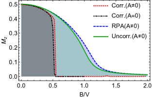
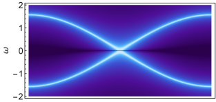
In absence of the spin bath (A=0𝐴0A=0), the phase diagram does not change much with respect to the uncorrelated result. The critical field Bcsubscript𝐡𝑐B_{c} shifts towards slightly larger values, stabilizing the ferromagnetic phase. On the other hand, this approximation captures that, at the quantum phase transition, the magnon gap closes, as it can be seen in the spin-spin correlation function (Fig.2, top).
Refer to caption
Refer to caption
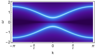
Figure 2: Complex part of the bosonic Green’s function Gk,kz,z​(Ο‰)superscriptsubscriptπΊπ‘˜π‘˜π‘§π‘§πœ”G_{k,k}^{z,z}\left(\omega\right) as a function of kπ‘˜k and Ο‰πœ”\omega. (Top) In absence of the spin bath, the magnon gap closes at the critical point Bc≃1.1​Vsimilar-to-or-equalssubscript𝐡𝑐1.1𝑉B_{c}\simeq 1.1V. (Bottom) Gap does not close at the critical point if the longitudinal coupling to the bath is included. We have considered A=0.05​V𝐴0.05𝑉A=0.05V and a 1D lattice with ZB=ZB​S=1subscript𝑍𝐡subscript𝑍𝐡𝑆1Z_{B}=Z_{BS}=1. The results are expressed in logarithmic scale to enhance the contrast.

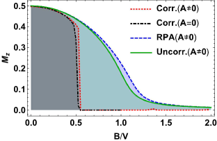
When the spin bath is included (Aβ‰ 0𝐴0A\neq 0), the difference between the uncorrelated and correlated phase diagrams gets reduced (see Fig.3, green and blue lines). The reason is that two-point correlations between Ising spins dominate near the unperturbed Ising critical point, which is now shifted. This can be seen in Fig.3, where the main differences happen near the Ising critical point Bc≃1.1​Vsimilar-to-or-equalssubscript𝐡𝑐1.1𝑉B_{c}\simeq 1.1V, and the two solutions match again for larger B𝐡B. Therefore, spin-spin correlations do not change quantitatively the phase diagram, in the presence of the spin bath.
Refer to caption
Figure 3: Mzsubscript𝑀𝑧M_{z} vs B/V𝐡𝑉B/V for the Ising model longitudinally coupled to a bath of spins at T=0𝑇0T=0. (Green) Uncorrelated solution for A=0.05​V𝐴0.05𝑉A=0.05V and ZB=1subscript𝑍𝐡1Z_{B}=1. (Blue) RPA solution including for A=0.05​V𝐴0.05𝑉A=0.05V and ZB=1subscript𝑍𝐡1Z_{B}=1. (Black) Solution including correlated parts without the spin bath (A=0𝐴0A=0). (Red) Solution including correlations for a large spin bath (A=0.2​V𝐴0.2𝑉A=0.2V and ZB=100subscript𝑍𝐡100Z_{B}=100).

On the other hand, the effect of the bath in the correlation functions is more crucial, as it leads to a mode softening at the critical point. Without the spin bath, the magnon gap closes, signaling a divergence of the correlation length between Ising spins; however, the presence of the remnant field produced by the spin bath makes the gap finite for all B𝐡B, and the correlation length between spins remains finite. Furthermore, the effect of a dynamical bath due to a transverse field Ξ”β‰ 0Ξ”0\Delta\neq 0 modifies this picture non-trivially. The fact that Eq.17 corresponds to Ising magnons under an effective longitudinal field ∼ZB​A​mzsimilar-toabsentsubscript𝑍𝐡𝐴subscriptπ‘šπ‘§\sim Z_{B}Am_{z} is not a coincidence. When the bath is static (Ξ”=0Ξ”0\Delta=0), system and bath do not get entangled, but making the bath dynamical (Ξ”β‰ 0Ξ”0\Delta\neq 0) correlates both systems and modifies the quasiparticle picture. Fig.4 shows the appearance of an electro-nuclear mode with non-vanishing spectral weight. This mode emerges near ω≃0similar-to-or-equalsπœ”0\omega\simeq 0 when κ≑ZB​ZB​S​A2​B​Δ​mx​Mxβ‰ 0πœ…subscript𝑍𝐡subscript𝑍𝐡𝑆superscript𝐴2𝐡Δsubscriptπ‘šπ‘₯subscript𝑀π‘₯0\kappa\equiv Z_{B}Z_{BS}A^{2}B\Delta m_{x}M_{x}\neq 0 and corresponds to a mixture of magnon and bath excitation, as it can be seen from the poles of the Green’s function:

Ο‰~k=Β±Ξ©2+Ο‰k22Β±ΞΊ+(Ξ©2βˆ’Ο‰k22)2subscript~πœ”π‘˜plus-or-minusplus-or-minussuperscriptΞ©2superscriptsubscriptπœ”π‘˜22πœ…superscriptsuperscriptΞ©2superscriptsubscriptπœ”π‘˜222\tilde{\omega}_{k}=\pm\sqrt{\frac{\Omega^{2}+\omega_{k}^{2}}{2}\pm\sqrt{\kappa+\left(\frac{\Omega^{2}-\omega_{k}^{2}}{2}\right)^{2}}} (20)

where Ξ©=Ξ”2+ZB​S2​A2Ξ©superscriptΞ”2superscriptsubscript𝑍𝐡𝑆2superscript𝐴2\Omega=\sqrt{\Delta^{2}+Z_{BS}^{2}A^{2}} (details in the Appendix). The presence of this mode has been observed in (LiHoFPhaseTransition, ) and discussed in detail in ref.(Ryan-Spinbath, ). There it is shown that this mode does not carry spectral weight unless the bath is dynamical, and that it allows to recover the QCP.
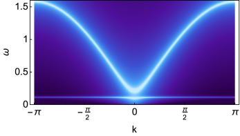
Refer to caption
Figure 4: Emergence of an electro-nuclear mode at the critical point when system and bath get correlated due to a finite Ξ”=10βˆ’3​BΞ”superscript103𝐡\Delta=10^{-3}B.

Finally, we discuss the impact of adding the correlated parts in the equation of motion. As previously mentioned, their effect can be incorporated in terms of a self-energy, but in the general case, the self-energy will be a complicated function of frequency and momentum. To estimate their effect we analyze the longitudinal magnetization, which can be addressed more easily by using the Majorana representation for spins(MajoranaRep, ):

SΞ±=βˆ’i2​ϡα​θ1​θ2​ηθ1​ηθ2superscript𝑆𝛼𝑖2subscriptitalic-ϡ𝛼subscriptπœƒ1subscriptπœƒ2superscriptπœ‚subscriptπœƒ1superscriptπœ‚subscriptπœƒ2S^{\alpha}=-\frac{i}{2}\epsilon_{\alpha\theta_{1}\theta_{2}}\eta^{\theta_{1}}\eta^{\theta_{2}} (21)

This representation simplifies the self-consistency equations, and makes the self-energy for the longitudinal magnetization Ξ£z​z​(kβ†’,Ο‰)superscriptΞ£π‘§π‘§β†’π‘˜πœ”\Sigma^{zz}\left(\vec{k},\omega\right) a function of Ο‰πœ”\omega only. Furthermore, unlike the Wigner-Jordan transformation, this representation is local and the separation between correlated and uncorrelated parts is analogous to the spins case. The derivation of the equations of motion, as well as the decoupling scheme is analogous to the case of the spin representation, as described in the Appendix.

The phase diagram including the correlated parts is shown in Fig.3. In absence of the spin bath (A=0𝐴0A=0, black line), the ferromagnetic phase shrinks and the QCP shifts to B/V≃1/2similar-to-or-equals𝐡𝑉12B/V\simeq 1/2, which is the exact result for the 1D Ising model. When the spin bath is included (Aβ‰ 0𝐴0A\neq 0, red line), the phase boundary shifts towards larger values of B/V𝐡𝑉B/V, as it happened in the uncorrelated phase diagram. However, in this case the remnant magnetic field produced by the spin bath is highly renormalized by the correlated parts. This can be seen from the specific values chosen for the bath in Fig.3 (A=0.2​V𝐴0.2𝑉A=0.2V and ZB=100subscript𝑍𝐡100Z_{B}=100), which for the uncorrelated solution would produce a phase boundary shifted towards much larger values of B/V𝐡𝑉B/V. Importantly, although the QPT seems to be recovered when correlated parts are included, this is not the case. One can check that Mz​(T=0)=0subscript𝑀𝑧𝑇00M_{z}\left(T=0\right)=0 is not a fixed point of the self-consistency equations, although its final value is very small due to the large renormalization.

Conclusions:

We have shown that a large variety of spin models interacting with spin baths can be treated using the equation of motion technique. This approach allows for non-perturbative solutions, even to lowest order, and using our decoupling scheme one can include corrections in a systematic way. Neglecting correlations yields the standard MF solution, while adding the lowest order correlations between pairs of spins reproduces the RPA results.

As a concrete example, we have analyzed the Quantum Ising model coupled to a local bath of spins, where each Ising spin is coupled to a set of ZBsubscript𝑍𝐡Z_{B} independent spins. This case is interesting due to the changes produced by the longitudinal interaction on the critical properties. In the absence of correlations we have obtained solutions for arbitrary spin value in the bath, and demonstrated that a remnant magnetic field produced by the bath can block the quantum phase transition. When correlations are included, system and bath quasiparticles can mix, transforming the standard magnons into electro-nuclear modes. We have shown that the effect of internal dynamics in the spin bath entangles the system and bath spins, and that this leads to the emergence of electro-nuclear modes near the phase transition.

When higher correlations are added (i.e., the correlated parts of the Green’s functions), some quantities are accurately captured. For the Quantum Ising model we have obtained the exact critical point in 1D and shown that the effect of the spin bath gets highly renormalized by the virtual processes.

Future directions for this work include the study of more complicated spin models, as for example with transverse terms and dipolar interactions, or considering more complex connectivity between bath and system (e.g., if a bath spin can interact with more than a single Ising spin, the results would appreciably change). To conclude, effective models of spin systems interacting with localized modes are ubiquitous in experiments at low temperature. Some examples are: dangling bonds DanglingBonds , nuclear spins LiHoFPhaseTransition ; MorelloNuclearSpinBathSingleMolecule ; Nuclearspinbathquantumdots , paramagnetic impurities ParamagneticImpurities ; ParamagneticImpuritiesII , and localized vibrational modes Discretphononmodes . Therefore a a theoretical approach that allows to systematically study them is very relevant for the field.

We would like to thank R. D. McKenzie for helpful discussions. This work was supported by the National Scientific and Engineering Research Council of Canada and A.G-L. acknowledges the Juan de la Cierva program.

References

  • (1) E.Β B.-N. P.L.Β Krapivsky, S.Β Redner, A Kinetic View of Statistical Physics, Cambridge University Press, 2010.
  • (2) S.Β Lloyd, J. Phys.: Conf. Ser. 302, 012037 (2011).
  • (3) H.Β G. Hiscock etΒ al., Proceedings of the National Academy of Sciences (2016).
  • (4) A.Β Das and B.Β K. Chakrabarti, Rev. Mod. Phys. 80, 1061 (2008).
  • (5) K.Β Sengupta, S.Β Powell, and S.Β Sachdev, Phys. Rev. A 69, 053616 (2004).
  • (6) S.Β Sachdev, Quantum Phase Transitions, Cambridge University Press, 2 edition, 2011.
  • (7) H.Β M. RΓΈnnow etΒ al., Science 308, 389 (2005).
  • (8) M.Β Schechter and P.Β C.Β E. Stamp, Phys. Rev. Lett. 95, 267208 (2005).
  • (9) N.Β V. Prokof’ev and P.Β C.Β E. Stamp, Reports on Progress in Physics 63, 669 (2000).
  • (10) S.Β Boixo etΒ al., Nature Physics 10, 218 (2014).
  • (11) R.Β Barends etΒ al., Nature 534, 222 (2016).
  • (12) E.Β F. Dumitrescu etΒ al., Phys. Rev. Lett. 120, 210501 (2018).
  • (13) S.Β Tomsovic, Proceedings from the Institute for Nuclear Theory-Vol.5: Tunneling in complex systems, World Scientific Pub Co Inc, 1998.
  • (14) J.Β M. Martinis etΒ al., Phys. Rev. Lett. 95, 210503 (2005).
  • (15) C.Β Deng and X.Β Hu, Phys. Rev. B 73, 241303 (2006).
  • (16) D.Β Zubarev, Soviet Physics Uspekhi 3, 320 (1960).
  • (17) H.-Y. WANG, K.-Q. CHEN, and E.-G. WANG, International Journal of Modern Physics B 16, 3803 (2002).
  • (18) J.Β Schreiber, Physica B+C 96, 27 (1979).
  • (19) A.Β GΓ³mez-LeΓ³n, Phys. Rev. B 96, 064426 (2017).
  • (20) A.Β GΓ³mez-LeΓ³n, Phys. Rev. B 94, 035144 (2016).
  • (21) J.Β H. Page, S.Β R.Β P. Smith, and D.Β R. Taylor, Journal of Physics C: Solid State Physics 17, 73 (1984).
  • (22) R.Β D. McKenzie and P.Β C.Β E. Stamp, Phys. Rev. B 97, 214430 (2018).
  • (23) V.Β R. Vieira, Phys. Rev. B 23, 6043 (1981).
  • (24) A.Β M. Holder, K.Β D. Osborn, C.Β Lobb, and C.Β B. Musgrave, Physical review letters 111, 065901 (2013).
  • (25) A.Β Morello, O.Β N. Bakharev, H.Β B. Brom, R.Β Sessoli, and L.Β J. deΒ Jongh, Phys. Rev. Lett. 93, 197202 (2004).
  • (26) E.Β Chekhovich etΒ al., Nature materials 12, 494 (2013).
  • (27) L.Β Luan etΒ al., Scientific reports 5, 8119 (2015).
  • (28) C.Β M. Quintana etΒ al., Phys. Rev. Lett. 118, 057702 (2017).
  • (29) J.Β Lisenfeld etΒ al., Scientific reports 6, 23786 (2016).

Appendix A Comparison between the uncorrelated and the exact solution for two spins

Here we discuss the limitations of the uncorrelated solution in terms of a two spin system. Consider the next Hamiltonian:

H=βˆ’Bx​Sxβˆ’Bz​Szβˆ’Ξ”z​Iz+A​Iz​Sz𝐻subscript𝐡π‘₯superscript𝑆π‘₯subscript𝐡𝑧superscript𝑆𝑧subscriptΔ𝑧superscript𝐼𝑧𝐴superscript𝐼𝑧superscript𝑆𝑧H=-B_{x}S^{x}-B_{z}S^{z}-\Delta_{z}I^{z}+AI^{z}S^{z} (22)

where a single spin is coupled to a single bath spin. The interaction between the two spins is longitudinal and proportional to A𝐴A. In addition, the Ising spin has a longitudinal field Bzsubscript𝐡𝑧B_{z} which mimics the effect of the field produced by all the other Ising spins in the Ising model, and a transverse field Bxsubscript𝐡π‘₯B_{x}. Also the bath spin can be biased by a longitudinal field Ξ”zsubscriptΔ𝑧\Delta_{z}. The exact calculation is possible due to the small size of the Hilbert space, and the statistical average for the magnetization of the Ising spin can be obtained analytically:

Mz=Zβˆ’1​Tr​{eβˆ’HT​Sz}subscript𝑀𝑧superscript𝑍1Trsuperscript𝑒𝐻𝑇superscript𝑆𝑧\displaystyle M_{z}=Z^{-1}\textrm{Tr}\left\{e^{-\frac{H}{T}}S^{z}\right\} =\displaystyle= eβˆ’Ξ”2​T​(A+2​Bz)​sinh⁑((A+2​Bz)2+4​B24​T)Z​(A+2​Bz)2+4​B2βˆ’eΞ”2​T​(Aβˆ’2​Bz)​sinh⁑((Aβˆ’2​Bz)2+4​B24​T)Z​(Aβˆ’2​Bz)2+4​B2superscript𝑒Δ2𝑇𝐴2subscript𝐡𝑧superscript𝐴2subscript𝐡𝑧24superscript𝐡24𝑇𝑍superscript𝐴2subscript𝐡𝑧24superscript𝐡2superscript𝑒Δ2𝑇𝐴2subscript𝐡𝑧superscript𝐴2subscript𝐡𝑧24superscript𝐡24𝑇𝑍superscript𝐴2subscript𝐡𝑧24superscript𝐡2\displaystyle e^{-\frac{\Delta}{2T}}\left(A+2B_{z}\right)\frac{\sinh\left(\frac{\sqrt{\left(A+2B_{z}\right)^{2}+4B^{2}}}{4T}\right)}{Z\sqrt{\left(A+2B_{z}\right)^{2}+4B^{2}}}-e^{\frac{\Delta}{2T}}\left(A-2B_{z}\right)\frac{\sinh\left(\frac{\sqrt{\left(A-2B_{z}\right)^{2}+4B^{2}}}{4T}\right)}{Z\sqrt{\left(A-2B_{z}\right)^{2}+4B^{2}}} (23)

where

Z=2​eΞ”2​T​cosh⁑((Aβˆ’2​Bz)2+4​Bx24​T)+2​eβˆ’Ξ”2​T​cosh⁑((A+2​Bz)2+4​Bx24​T)𝑍2superscript𝑒Δ2𝑇superscript𝐴2subscript𝐡𝑧24superscriptsubscript𝐡π‘₯24𝑇2superscript𝑒Δ2𝑇superscript𝐴2subscript𝐡𝑧24superscriptsubscript𝐡π‘₯24𝑇Z=2e^{\frac{\Delta}{2T}}\cosh\left(\frac{\sqrt{\left(A-2B_{z}\right)^{2}+4B_{x}^{2}}}{4T}\right)+2e^{-\frac{\Delta}{2T}}\cosh\left(\frac{\sqrt{\left(A+2B_{z}\right)^{2}+4B_{x}^{2}}}{4T}\right) (24)

is the partition function. On the other hand, we make use of the self-consistency equations for the magnetization, obtained from the uncorrelated solutions of the Green’s functions in the main text:

Mzsubscript𝑀𝑧\displaystyle M_{z} =\displaystyle= Bzβˆ’A​mz2​Bx2+(Bzβˆ’A​mz)2​tanh⁑(Bx2+(Bzβˆ’A​mz)22​T)subscript𝐡𝑧𝐴subscriptπ‘šπ‘§2superscriptsubscript𝐡π‘₯2superscriptsubscript𝐡𝑧𝐴subscriptπ‘šπ‘§2superscriptsubscript𝐡π‘₯2superscriptsubscript𝐡𝑧𝐴subscriptπ‘šπ‘§22𝑇\displaystyle\frac{B_{z}-Am_{z}}{2\sqrt{B_{x}^{2}+\left(B_{z}-Am_{z}\right)^{2}}}\tanh\left(\frac{\sqrt{B_{x}^{2}+\left(B_{z}-Am_{z}\right)^{2}}}{2T}\right) (25)
Mxsubscript𝑀π‘₯\displaystyle M_{x} =\displaystyle= Bx2​Bx2+(Bzβˆ’A​mz)2​tanh⁑(Bx2+(Bzβˆ’A​mz)22​T)subscript𝐡π‘₯2superscriptsubscript𝐡π‘₯2superscriptsubscript𝐡𝑧𝐴subscriptπ‘šπ‘§2superscriptsubscript𝐡π‘₯2superscriptsubscript𝐡𝑧𝐴subscriptπ‘šπ‘§22𝑇\displaystyle\frac{B_{x}}{2\sqrt{B_{x}^{2}+\left(B_{z}-Am_{z}\right)^{2}}}\tanh\left(\frac{\sqrt{B_{x}^{2}+\left(B_{z}-Am_{z}\right)^{2}}}{2T}\right) (26)
mzsubscriptπ‘šπ‘§\displaystyle m_{z} =\displaystyle= Ξ”zβˆ’A​Mz2​(Ξ”zβˆ’A​Mz)2​tanh⁑((Ξ”zβˆ’A​Mz)22​T)subscriptΔ𝑧𝐴subscript𝑀𝑧2superscriptsubscriptΔ𝑧𝐴subscript𝑀𝑧2superscriptsubscriptΔ𝑧𝐴subscript𝑀𝑧22𝑇\displaystyle\frac{\Delta_{z}-AM_{z}}{2\sqrt{\left(\Delta_{z}-AM_{z}\right)^{2}}}\tanh\left(\frac{\sqrt{\left(\Delta_{z}-AM_{z}\right)^{2}}}{2T}\right) (27)

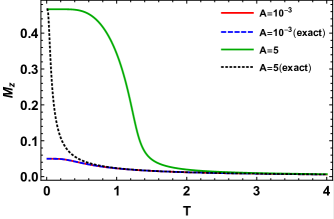
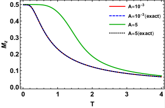
The comparison between the two solutions is shown in Fig.5. It shows that in the absence of a transverse field (Bx≃0similar-to-or-equalssubscript𝐡π‘₯0B_{x}\simeq 0) the longitudinal bath does not affect the Curie temperature, which is missed by the uncorrelated solution. On the other hand, for non-vanishing transverse field (i.e., when the Ising model becomes β€œquantum”), the bath modifies the behavior with temperature, specially in the low temperature regime.

Notice that the exact solution in terms of Green’s functions is also possible in this case, by just including the correlated part. This indicates that the intermediate temperature regime needs to be characterized including correlations (as one would expect, specially at the Curie temperature, where the correlation length diverges).
Refer to caption
Refer to caption
Figure 5: Comparison between the self-consistent solution and the exact calculation. (Left) Case with Bz=0.1subscript𝐡𝑧0.1B_{z}=0.1 and Bx=1subscript𝐡π‘₯1B_{x}=1, and (right) case with Bz=1subscript𝐡𝑧1B_{z}=1 and Bx=0.1subscript𝐡π‘₯0.1B_{x}=0.1. In general, the uncorrelated solution and the exact one, perfectly agree at low and high temperature, while for intermediate values they differ (for weak A𝐴A they agree very well in general). When the system is in the analog of a FM phase, with Bxβ‰ͺBzmuch-less-thansubscript𝐡π‘₯subscript𝐡𝑧B_{x}\ll B_{z} (right), the hyperfine coupling (even for large A𝐴A) would not make an important change in the Curie temperature (which happens for intermediate values of T𝑇T). This is in contrast with the case Bx≫Bzmuch-greater-thansubscript𝐡π‘₯subscript𝐡𝑧B_{x}\gg B_{z} (left), where specially at low T𝑇T the cases with small and large A𝐴A are quite different.

Appendix B Quantum Ising model coupled to a spin bath

The case of the Quantum Ising model is obtained from the general equation of motion by setting By,z=0subscript𝐡𝑦𝑧0B_{y,z}=0, Vi,jx,y=0superscriptsubscript𝑉𝑖𝑗π‘₯𝑦0V_{i,j}^{x,y}=0, Ξ”x,y=0subscriptΞ”π‘₯𝑦0\Delta_{x,y}=0 and Ai,lx,y=0superscriptsubscript𝐴𝑖𝑙π‘₯𝑦0A_{i,l}^{x,y}=0. Furthermore, if the bath spins are static (Ξ”β†’=0β†’Ξ”0\vec{\Delta}=0), it is useful to consider for its basis the set of eigenstates |P,Pz⟩ket𝑃subscript𝑃𝑧|P,P_{z}\rangle, where P𝑃P labels the spin value P∈[|Pβ†’|,|Pβ†’|βˆ’1,…,1/2]𝑃→𝑃→𝑃1…12P\in\left[\left|\vec{P}\right|,\left|\vec{P}\right|-1,\ldots,1/2\right] and Pz∈[P,Pβˆ’1,…,βˆ’P]subscript𝑃𝑧𝑃𝑃1…𝑃P_{z}\in\left[P,P-1,\ldots,-P\right] its projection. Their equation of motion is calculated analogously, from the Heisenberg equation:

βˆ‚tO^=i​[H,O^]subscript𝑑^𝑂𝑖𝐻^𝑂\partial_{t}\hat{O}=i\left[H,\hat{O}\right] (28)

The advantage of using this basis is that it allows to calculate the solutions for arbitrary spin value. The Hamiltonian reads in this basis:

HS=βˆ’Bβ€‹βˆ‘iSixβˆ’βˆ‘i,j>iVi,j​Siz​Sjzβˆ’Ξ”zβ€‹βˆ‘lβˆ‘P,PzPz​XP,lPz,Pz+βˆ‘i,lAi,l​Sizβ€‹βˆ‘P,PzPz​XP,lPz,Pzsubscript𝐻𝑆𝐡subscript𝑖superscriptsubscript𝑆𝑖π‘₯subscript𝑖𝑗𝑖subscript𝑉𝑖𝑗superscriptsubscript𝑆𝑖𝑧superscriptsubscript𝑆𝑗𝑧subscriptΔ𝑧subscript𝑙subscript𝑃subscript𝑃𝑧subscript𝑃𝑧superscriptsubscript𝑋𝑃𝑙subscript𝑃𝑧subscript𝑃𝑧subscript𝑖𝑙subscript𝐴𝑖𝑙superscriptsubscript𝑆𝑖𝑧subscript𝑃subscript𝑃𝑧subscript𝑃𝑧superscriptsubscript𝑋𝑃𝑙subscript𝑃𝑧subscript𝑃𝑧H_{S}=-B\sum_{i}S_{i}^{x}-\sum_{i,j>i}V_{i,j}S_{i}^{z}S_{j}^{z}-\Delta_{z}\sum_{l}\sum_{P,P_{z}}P_{z}X_{P,l}^{P_{z},P_{z}}+\sum_{i,l}A_{i,l}S_{i}^{z}\sum_{P,P_{z}}P_{z}X_{P,l}^{P_{z},P_{z}} (29)

where

XP,lPz,Pz=|P,Pz⟩lβ€‹βŸ¨P,Pz|lsuperscriptsubscript𝑋𝑃𝑙subscript𝑃𝑧subscript𝑃𝑧subscriptket𝑃subscript𝑃𝑧𝑙subscriptbra𝑃subscript𝑃𝑧𝑙X_{P,l}^{P_{z},P_{z}}=|P,P_{z}\rangle_{l}\langle P,P_{z}|_{l}

is the projector onto the eigenstate of the bath at site l𝑙l. Neglecting correlations one finds that the average value of each projector, and the magnetization mnz=βˆ‘Pz,PPzβ€‹βŸ¨XP,nPz,Pz⟩superscriptsubscriptπ‘šπ‘›π‘§subscriptsubscript𝑃𝑧𝑃subscript𝑃𝑧delimited-⟨⟩superscriptsubscript𝑋𝑃𝑛subscript𝑃𝑧subscript𝑃𝑧m_{n}^{z}=\sum_{P_{z},P}P_{z}\langle X_{P,n}^{P_{z},P_{z}}\rangle are given by:

⟨XP,na,a⟩delimited-⟨⟩superscriptsubscriptπ‘‹π‘ƒπ‘›π‘Žπ‘Ž\displaystyle\langle X_{P,n}^{a,a}\rangle =\displaystyle= e(aβˆ’1)​hbT2​(ehbTβˆ’1)2cosh⁑[hbT​(|Pβ†’|+1)]βˆ’cosh⁑(hb2​T)superscriptπ‘’π‘Ž1subscriptβ„Žπ‘π‘‡2superscriptsuperscript𝑒subscriptβ„Žπ‘π‘‡12subscriptβ„Žπ‘π‘‡β†’π‘ƒ1subscriptβ„Žπ‘2𝑇\displaystyle\frac{e^{\left(a-1\right)\frac{h_{b}}{T}}}{2}\frac{\left(e^{\frac{h_{b}}{T}}-1\right)^{2}}{\cosh\left[\frac{h_{b}}{T}\left(\left|\vec{P}\right|+1\right)\right]-\cosh\left(\frac{h_{b}}{2T}\right)} (30)
mnzsuperscriptsubscriptπ‘šπ‘›π‘§\displaystyle m_{n}^{z} =\displaystyle= βˆ’14​csch​(hb2​T)​3+cosh⁑(hbT)βˆ’2​(2+|Pβ†’|)​cosh⁑[hb2​T​(1+2​|Pβ†’|)]+2​|Pβ†’|​cosh⁑[hb2​T​(3+2​|Pβ†’|)]cosh⁑(hb2​T)βˆ’cosh⁑[hbT​(|Pβ†’|+1)]14cschsubscriptβ„Žπ‘2𝑇3subscriptβ„Žπ‘π‘‡22→𝑃subscriptβ„Žπ‘2𝑇12→𝑃2→𝑃subscriptβ„Žπ‘2𝑇32→𝑃subscriptβ„Žπ‘2𝑇subscriptβ„Žπ‘π‘‡β†’π‘ƒ1\displaystyle-\frac{1}{4}\text{csch}\left(\frac{h_{b}}{2T}\right)\frac{3+\cosh\left(\frac{h_{b}}{T}\right)-2\left(2+\left|\vec{P}\right|\right)\cosh\left[\frac{h_{b}}{2T}\left(1+2\left|\vec{P}\right|\right)\right]+2\left|\vec{P}\right|\cosh\left[\frac{h_{b}}{2T}\left(3+2\left|\vec{P}\right|\right)\right]}{\cosh\left(\frac{h_{b}}{2T}\right)-\cosh\left[\frac{h_{b}}{T}\left(\left|\vec{P}\right|+1\right)\right]} (31)

where hb​(n)=Ξ”zβˆ’βˆ‘iAi,n​Mizsubscriptβ„Žπ‘π‘›subscriptΔ𝑧subscript𝑖subscript𝐴𝑖𝑛superscriptsubscript𝑀𝑖𝑧h_{b}\left(n\right)=\Delta_{z}-\sum_{i}A_{i,n}M_{i}^{z}. This solution is specific for half-integer spins, but the case for integer spins can be calculated analogously. Finally, we use the solution for the fermionic Green’s function to obtain the self-consistency equations for the magnetization:

Mzsubscript𝑀𝑧\displaystyle M_{z} =\displaystyle= hs2​ωs​tanh⁑(Ο‰s2​T)subscriptβ„Žπ‘ 2subscriptπœ”π‘ subscriptπœ”π‘ 2𝑇\displaystyle\frac{h_{s}}{2\omega_{s}}\tanh\left(\frac{\omega_{s}}{2T}\right) (32)
Mxsubscript𝑀π‘₯\displaystyle M_{x} =\displaystyle= B2​ωs​tanh⁑(Ο‰s2​T)𝐡2subscriptπœ”π‘ subscriptπœ”π‘ 2𝑇\displaystyle\frac{B}{2\omega_{s}}\tanh\left(\frac{\omega_{s}}{2T}\right) (33)

With these results one can now estimate the Curie temperature and the critical field. For the Curie temperature we are looking for solutions with B=0𝐡0B=0. We consider the case where the bath is unbiased by an external field to simplify the expressions (Ξ”z=0subscriptΔ𝑧0\Delta_{z}=0). Expanding for small Mzsubscript𝑀𝑧M_{z} up to third order, and solving for the value of T𝑇T that makes Mz=0subscript𝑀𝑧0M_{z}=0, we find:

Tcsubscript𝑇𝑐\displaystyle T_{c} =\displaystyle= V08+14​(V02)2+ZB​ZB​S​A2​1+8​|Pβ†’|+4​|Pβ†’|26subscript𝑉0814superscriptsubscript𝑉022subscript𝑍𝐡subscript𝑍𝐡𝑆superscript𝐴218→𝑃4superscript→𝑃26\displaystyle\frac{V_{0}}{8}+\frac{1}{4}\sqrt{\left(\frac{V_{0}}{2}\right)^{2}+Z_{B}Z_{BS}A^{2}\frac{1+8\left|\vec{P}\right|+4\left|\vec{P}\right|^{2}}{6}} (34)

It shows that for this approximation, the Curie temperature would increase with all the coordination numbers (remember V0=Zs​Vsubscript𝑉0subscript𝑍𝑠𝑉V_{0}=Z_{s}V), as well as with the total spin of the bath |Pβ†’|→𝑃\left|\vec{P}\right| . As discussed in the previous section of the Appendix, this result is not correct for a local spin bath, because the Curie temperature should not be affected by the longitudinally coupled bath. The correction is provided by the correlations between the Ising spins and the bath spins. On the other hand, this model can also have several Ising spins coupled to each bath spin, and in this case the Curie temperature can be affected. Similarly for the critical field one finds:

Mz≃ZB​A​|Pβ†’|2​B2+A2​|Pβ†’|2​ZB2+B2​V0​Mz2​[B2+A2​|Pβ†’|2​ZB2]3/2+π’ͺ​(Mz2)similar-to-or-equalssubscript𝑀𝑧subscript𝑍𝐡𝐴→𝑃2superscript𝐡2superscript𝐴2superscript→𝑃2superscriptsubscript𝑍𝐡2superscript𝐡2subscript𝑉0subscript𝑀𝑧2superscriptdelimited-[]superscript𝐡2superscript𝐴2superscript→𝑃2superscriptsubscript𝑍𝐡232π’ͺsuperscriptsubscript𝑀𝑧2M_{z}\simeq\frac{Z_{B}A\left|\vec{P}\right|}{2\sqrt{B^{2}+A^{2}\left|\vec{P}\right|^{2}Z_{B}^{2}}}+\frac{B^{2}V_{0}M_{z}}{2\left[B^{2}+A^{2}\left|\vec{P}\right|^{2}Z_{B}^{2}\right]^{3/2}}+\mathcal{O}\left(M_{z}^{2}\right) (35)

Then Mz=0subscript𝑀𝑧0M_{z}=0 is not a solution due to a remnant magnetization, which saturates for large A≫Bmuch-greater-than𝐴𝐡A\gg B.

Appendix C Effect of two-spin correlations

In order to include two-point correlations, we include the Fock term in the equation of motion. This couples Green’s functions at different lattice sites:

ω​Gn,mΞ±,Ξ²πœ”superscriptsubscriptπΊπ‘›π‘šπ›Όπ›½\displaystyle\omega G_{n,m}^{\alpha,\beta} =\displaystyle= ⟨[SnΞ±,OmΞ²]±⟩+iβ€‹βˆ‘ΞΌΟ΅ΞΌβ€‹Ξ±β€‹Οβ€‹(BΞΌ+βˆ‘iβ‰ nVi,nμ​MiΞΌβˆ’βˆ‘lAn,lμ​mlΞΌ)​Gn,mρ,Ξ²delimited-⟨⟩subscriptsuperscriptsubscript𝑆𝑛𝛼superscriptsubscriptπ‘‚π‘šπ›½plus-or-minus𝑖subscriptπœ‡subscriptitalic-Ο΅πœ‡π›ΌπœŒsubscriptπ΅πœ‡subscript𝑖𝑛superscriptsubscriptπ‘‰π‘–π‘›πœ‡superscriptsubscriptπ‘€π‘–πœ‡subscript𝑙superscriptsubscriptπ΄π‘›π‘™πœ‡superscriptsubscriptπ‘šπ‘™πœ‡superscriptsubscriptπΊπ‘›π‘šπœŒπ›½\displaystyle\langle\left[S_{n}^{\alpha},O_{m}^{\beta}\right]_{\pm}\rangle+i\sum_{\mu}\epsilon_{\mu\alpha\rho}\left(B_{\mu}+\sum_{i\neq n}V_{i,n}^{\mu}M_{i}^{\mu}-\sum_{l}A_{n,l}^{\mu}m_{l}^{\mu}\right)G_{n,m}^{\rho,\beta}
+iβ€‹βˆ‘ΞΌΟ΅ΞΌβ€‹Ξ±β€‹Οβ€‹Mnρ​(βˆ‘iβ‰ nVi,nμ​Gi,mΞΌ,Ξ²βˆ’βˆ‘lAn,lμ​Yl,mΞΌ,Ξ²)𝑖subscriptπœ‡subscriptitalic-Ο΅πœ‡π›ΌπœŒsuperscriptsubscriptπ‘€π‘›πœŒsubscript𝑖𝑛superscriptsubscriptπ‘‰π‘–π‘›πœ‡superscriptsubscriptπΊπ‘–π‘šπœ‡π›½subscript𝑙superscriptsubscriptπ΄π‘›π‘™πœ‡superscriptsubscriptπ‘Œπ‘™π‘šπœ‡π›½\displaystyle+i\sum_{\mu}\epsilon_{\mu\alpha\rho}M_{n}^{\rho}\left(\sum_{i\neq n}V_{i,n}^{\mu}G_{i,m}^{\mu,\beta}-\sum_{l}A_{n,l}^{\mu}Y_{l,m}^{\mu,\beta}\right)
ω​Yn,mΞ±,Ξ²πœ”superscriptsubscriptπ‘Œπ‘›π‘šπ›Όπ›½\displaystyle\omega Y_{n,m}^{\alpha,\beta} =\displaystyle= ⟨[InΞ±,OmΞ²]±⟩+iβ€‹βˆ‘ΞΌΟ΅ΞΌβ€‹Ξ±β€‹Οβ€‹(Ξ”ΞΌβˆ’βˆ‘iAi,nΞΌβ€‹βŸ¨Siμ⟩)​Yn,mρ,Ξ²βˆ’iβ€‹βˆ‘ΞΌ,iϡμ​α​ρ​Ai,nΞΌβ€‹βŸ¨InΟβŸ©β€‹Gi,mΞΌ,Ξ²delimited-⟨⟩subscriptsuperscriptsubscript𝐼𝑛𝛼superscriptsubscriptπ‘‚π‘šπ›½plus-or-minus𝑖subscriptπœ‡subscriptitalic-Ο΅πœ‡π›ΌπœŒsubscriptΞ”πœ‡subscript𝑖superscriptsubscriptπ΄π‘–π‘›πœ‡delimited-⟨⟩superscriptsubscriptπ‘†π‘–πœ‡superscriptsubscriptπ‘Œπ‘›π‘šπœŒπ›½π‘–subscriptπœ‡π‘–subscriptitalic-Ο΅πœ‡π›ΌπœŒsuperscriptsubscriptπ΄π‘–π‘›πœ‡delimited-⟨⟩superscriptsubscriptπΌπ‘›πœŒsuperscriptsubscriptπΊπ‘–π‘šπœ‡π›½\displaystyle\langle\left[I_{n}^{\alpha},O_{m}^{\beta}\right]_{\pm}\rangle+i\sum_{\mu}\epsilon_{\mu\alpha\rho}\left(\Delta_{\mu}-\sum_{i}A_{i,n}^{\mu}\langle S_{i}^{\mu}\rangle\right)Y_{n,m}^{\rho,\beta}-i\sum_{\mu,i}\epsilon_{\mu\alpha\rho}A_{i,n}^{\mu}\langle I_{n}^{\rho}\rangle G_{i,m}^{\mu,\beta}

Using a transformation to momentum space, while assuming spatially homogeneous solutions, we find:

ω​GkΞ±,Ξ²πœ”superscriptsubscriptπΊπ‘˜π›Όπ›½\displaystyle\omega G_{k}^{\alpha,\beta} =\displaystyle= ⟨[SΞ±,OΞ²]±⟩+iβ€‹βˆ‘ΞΌΟ΅ΞΌβ€‹Ξ±β€‹Οβ€‹Ο‰s,μ​Gkρ,Ξ²+iβ€‹βˆ‘ΞΌΟ΅ΞΌβ€‹Ξ±β€‹Οβ€‹Mρ​(Vkμ​GkΞΌ,Ξ²βˆ’ZB​Aμ​YkΞΌ,Ξ²)delimited-⟨⟩subscriptsuperscript𝑆𝛼superscript𝑂𝛽plus-or-minus𝑖subscriptπœ‡subscriptitalic-Ο΅πœ‡π›ΌπœŒsubscriptπœ”π‘ πœ‡superscriptsubscriptπΊπ‘˜πœŒπ›½π‘–subscriptπœ‡subscriptitalic-Ο΅πœ‡π›ΌπœŒsubscriptπ‘€πœŒsuperscriptsubscriptπ‘‰π‘˜πœ‡superscriptsubscriptπΊπ‘˜πœ‡π›½subscript𝑍𝐡superscriptπ΄πœ‡superscriptsubscriptπ‘Œπ‘˜πœ‡π›½\displaystyle\langle\left[S^{\alpha},O^{\beta}\right]_{\pm}\rangle+i\sum_{\mu}\epsilon_{\mu\alpha\rho}\omega_{s,\mu}G_{k}^{\rho,\beta}+i\sum_{\mu}\epsilon_{\mu\alpha\rho}M_{\rho}\left(V_{k}^{\mu}G_{k}^{\mu,\beta}-Z_{B}A^{\mu}Y_{k}^{\mu,\beta}\right) (36)
ω​YkΞ±,Ξ²πœ”superscriptsubscriptπ‘Œπ‘˜π›Όπ›½\displaystyle\omega Y_{k}^{\alpha,\beta} =\displaystyle= ⟨[IΞ±,OΞ²]±⟩+iβ€‹βˆ‘ΞΌΟ΅ΞΌβ€‹Ξ±β€‹Οβ€‹Ο‰b,μ​Ykρ,Ξ²βˆ’iβ€‹βˆ‘ΞΌΟ΅ΞΌβ€‹Ξ±β€‹Οβ€‹mρ​ZB​S​Aμ​GkΞΌ,Ξ²delimited-⟨⟩subscriptsuperscript𝐼𝛼superscript𝑂𝛽plus-or-minus𝑖subscriptπœ‡subscriptitalic-Ο΅πœ‡π›ΌπœŒsubscriptπœ”π‘πœ‡superscriptsubscriptπ‘Œπ‘˜πœŒπ›½π‘–subscriptπœ‡subscriptitalic-Ο΅πœ‡π›ΌπœŒsubscriptπ‘šπœŒsubscript𝑍𝐡𝑆superscriptπ΄πœ‡superscriptsubscriptπΊπ‘˜πœ‡π›½\displaystyle\langle\left[I^{\alpha},O^{\beta}\right]_{\pm}\rangle+i\sum_{\mu}\epsilon_{\mu\alpha\rho}\omega_{b,\mu}Y_{k}^{\rho,\beta}-i\sum_{\mu}\epsilon_{\mu\alpha\rho}m_{\rho}Z_{BS}A^{\mu}G_{k}^{\mu,\beta} (37)

where Ο‰s,ΞΌ=BΞΌ+βˆ‘iβ‰ nV0μ​MΞΌβˆ’ZB​Aμ​mΞΌsubscriptπœ”π‘ πœ‡subscriptπ΅πœ‡subscript𝑖𝑛superscriptsubscript𝑉0πœ‡subscriptπ‘€πœ‡subscript𝑍𝐡superscriptπ΄πœ‡subscriptπ‘šπœ‡\omega_{s,\mu}=B_{\mu}+\sum_{i\neq n}V_{0}^{\mu}M_{\mu}-Z_{B}A^{\mu}m_{\mu} and Ο‰b,ΞΌ=Ξ”ΞΌβˆ’ZB​S​Aμ​MΞΌsubscriptπœ”π‘πœ‡subscriptΞ”πœ‡subscript𝑍𝐡𝑆superscriptπ΄πœ‡subscriptπ‘€πœ‡\omega_{b,\mu}=\Delta_{\mu}-Z_{BS}A^{\mu}M_{\mu}.

For the case of the Ising model longitudinally coupled to a bath of spins and Ξ”x=0subscriptΞ”π‘₯0\Delta_{x}=0, the poles of the Ising spins Green’s functions are at:

Ο‰ksubscriptπœ”π‘˜\displaystyle\omega_{k} =\displaystyle= B2+(Mz​V0βˆ’ZB​A​mz)2βˆ’B​Mx​Vksuperscript𝐡2superscriptsubscript𝑀𝑧subscript𝑉0subscript𝑍𝐡𝐴subscriptπ‘šπ‘§2𝐡subscript𝑀π‘₯subscriptπ‘‰π‘˜\displaystyle\sqrt{B^{2}+\left(M_{z}V_{0}-Z_{B}Am_{z}\right)^{2}-BM_{x}V_{k}} (38)

The corresponding self-consistency equations are obtained from the anti-commutator Green’s functions:

Mzsubscript𝑀𝑧\displaystyle M_{z} =\displaystyle= Mz​V0βˆ’ZB​A​mz2​1Nβ€‹βˆ‘kΟ‰k​coth⁑(Ο‰k2​T)subscript𝑀𝑧subscript𝑉0subscript𝑍𝐡𝐴subscriptπ‘šπ‘§21𝑁subscriptπ‘˜subscriptπœ”π‘˜hyperbolic-cotangentsubscriptπœ”π‘˜2𝑇\displaystyle\frac{M_{z}V_{0}-Z_{B}Am_{z}}{2\frac{1}{N}\sum_{k}\omega_{k}\coth\left(\frac{\omega_{k}}{2T}\right)} (39)
Mxsubscript𝑀π‘₯\displaystyle M_{x} =\displaystyle= B2​1Nβ€‹βˆ‘kΟ‰k​coth⁑(Ο‰k2​T)𝐡21𝑁subscriptπ‘˜subscriptπœ”π‘˜hyperbolic-cotangentsubscriptπœ”π‘˜2𝑇\displaystyle\frac{B}{2\frac{1}{N}\sum_{k}\omega_{k}\coth\left(\frac{\omega_{k}}{2T}\right)} (40)

If the bath is static one can see that the bath occupation probabilities are unchanged and that Ising spins and bath spins are not entangled.

If the bath has internal dynamics, now driven by Ξ”xβ‰ 0subscriptΞ”π‘₯0\Delta_{x}\neq 0, one finds that the poles are not simple Ising magnons anymore, but combinations of the bath and system excitations:

ω±=Ξ©2+Ο‰k22Β±ΞΊ+(Ξ©2βˆ’Ο‰k22)2subscriptπœ”plus-or-minusplus-or-minussuperscriptΞ©2superscriptsubscriptπœ”π‘˜22πœ…superscriptsuperscriptΞ©2superscriptsubscriptπœ”π‘˜222\omega_{\pm}=\sqrt{\frac{\Omega^{2}+\omega_{k}^{2}}{2}\pm\sqrt{\kappa+\left(\frac{\Omega^{2}-\omega_{k}^{2}}{2}\right)^{2}}} (41)

where ΞΊ=ZB​ZB​S​A2​Bx​Δx​mx​Mxπœ…subscript𝑍𝐡subscript𝑍𝐡𝑆superscript𝐴2subscript𝐡π‘₯subscriptΞ”π‘₯subscriptπ‘šπ‘₯subscript𝑀π‘₯\kappa=Z_{B}Z_{BS}A^{2}B_{x}\Delta_{x}m_{x}M_{x}, Ο‰k=Bx2+(Bz+V0​Mzβˆ’ZB​A​mz)2βˆ’Bx​Vk​Mxsubscriptπœ”π‘˜superscriptsubscript𝐡π‘₯2superscriptsubscript𝐡𝑧subscript𝑉0subscript𝑀𝑧subscript𝑍𝐡𝐴subscriptπ‘šπ‘§2subscript𝐡π‘₯subscriptπ‘‰π‘˜subscript𝑀π‘₯\omega_{k}=\sqrt{B_{x}^{2}+\left(B_{z}+V_{0}M_{z}-Z_{B}Am_{z}\right)^{2}-B_{x}V_{k}M_{x}} and Ξ©=Ξ”x2+(Ξ”zβˆ’ZB​S​A​Mz)Ξ©superscriptsubscriptΞ”π‘₯2subscriptΔ𝑧subscript𝑍𝐡𝑆𝐴subscript𝑀𝑧\Omega=\sqrt{\Delta_{x}^{2}+\left(\Delta_{z}-Z_{BS}AM_{z}\right)}. Analogously one can calculate the self-consistency equations for the magnetization, and the correlation functions:

Mzsubscript𝑀𝑧\displaystyle M_{z} =\displaystyle= Ο‰z2​ξ,Mx=Bx2​ξsubscriptπœ”π‘§2πœ‰subscript𝑀π‘₯subscript𝐡π‘₯2πœ‰\displaystyle\frac{\omega_{z}}{2\xi},\ M_{x}=\frac{B_{x}}{2\xi} (42)
ΞΎπœ‰\displaystyle\xi ≑\displaystyle\equiv 1Nβ€‹βˆ‘kΟ‰+β€‹Ο‰βˆ’β€‹(Ο‰+2βˆ’Ο‰βˆ’2)(1βˆ’Ξ»k)​[(Ξ©2βˆ’Ο‰βˆ’2)​ω+​tanh⁑(Ο‰βˆ’2​T)βˆ’(Ξ©2βˆ’Ο‰+2)β€‹Ο‰βˆ’β€‹tanh⁑(Ο‰+2​T)]1𝑁subscriptπ‘˜subscriptπœ”subscriptπœ”superscriptsubscriptπœ”2superscriptsubscriptπœ”21subscriptπœ†π‘˜delimited-[]superscriptΞ©2superscriptsubscriptπœ”2subscriptπœ”subscriptπœ”2𝑇superscriptΞ©2superscriptsubscriptπœ”2subscriptπœ”subscriptπœ”2𝑇\displaystyle\frac{1}{N}\sum_{k}\frac{\omega_{+}\omega_{-}\left(\omega_{+}^{2}-\omega_{-}^{2}\right)}{\left(1-\lambda_{k}\right)\left[\left(\Omega^{2}-\omega_{-}^{2}\right)\omega_{+}\tanh\left(\frac{\omega_{-}}{2T}\right)-\left(\Omega^{2}-\omega_{+}^{2}\right)\omega_{-}\tanh\left(\frac{\omega_{+}}{2T}\right)\right]}

where

Ξ»ksubscriptπœ†π‘˜\displaystyle\lambda_{k} =ZB​A​Δx​Mx​[Ο‰βˆ’β€‹tanh⁑(Ο‰+2​T)βˆ’Ο‰+​tanh⁑(Ο‰βˆ’2​T)](Ξ©2βˆ’Ο‰+2)β€‹Ο‰βˆ’β€‹tanh⁑(Ο‰+2​T)βˆ’(Ξ©2βˆ’Ο‰βˆ’2)​ω+​tanh⁑(Ο‰βˆ’2​T)absentsubscript𝑍𝐡𝐴subscriptΞ”π‘₯subscript𝑀π‘₯delimited-[]subscriptπœ”subscriptπœ”2𝑇subscriptπœ”subscriptπœ”2𝑇superscriptΞ©2superscriptsubscriptπœ”2subscriptπœ”subscriptπœ”2𝑇superscriptΞ©2superscriptsubscriptπœ”2subscriptπœ”subscriptπœ”2𝑇\displaystyle=\frac{Z_{B}A\Delta_{x}M_{x}\left[\omega_{-}\tanh\left(\frac{\omega_{+}}{2T}\right)-\omega_{+}\tanh\left(\frac{\omega_{-}}{2T}\right)\right]}{\left(\Omega^{2}-\omega_{+}^{2}\right)\omega_{-}\tanh\left(\frac{\omega_{+}}{2T}\right)-\left(\Omega^{2}-\omega_{-}^{2}\right)\omega_{+}\tanh\left(\frac{\omega_{-}}{2T}\right)}
Γ—ZB​S​A​Bx​mx​[Ο‰βˆ’β€‹tanh⁑(Ο‰+2​T)βˆ’Ο‰+​tanh⁑(Ο‰βˆ’2​T)](Ο‰k2βˆ’Ο‰+2)β€‹Ο‰βˆ’β€‹tanh⁑(Ο‰+2​T)βˆ’(Ο‰k2βˆ’Ο‰βˆ’2)​ω+​tanh⁑(Ο‰βˆ’2​T)absentsubscript𝑍𝐡𝑆𝐴subscript𝐡π‘₯subscriptπ‘šπ‘₯delimited-[]subscriptπœ”subscriptπœ”2𝑇subscriptπœ”subscriptπœ”2𝑇superscriptsubscriptπœ”π‘˜2superscriptsubscriptπœ”2subscriptπœ”subscriptπœ”2𝑇superscriptsubscriptπœ”π‘˜2superscriptsubscriptπœ”2subscriptπœ”subscriptπœ”2𝑇\displaystyle\times\frac{Z_{BS}AB_{x}m_{x}\left[\omega_{-}\tanh\left(\frac{\omega_{+}}{2T}\right)-\omega_{+}\tanh\left(\frac{\omega_{-}}{2T}\right)\right]}{\left(\omega_{k}^{2}-\omega_{+}^{2}\right)\omega_{-}\tanh\left(\frac{\omega_{+}}{2T}\right)-\left(\omega_{k}^{2}-\omega_{-}^{2}\right)\omega_{+}\tanh\left(\frac{\omega_{-}}{2T}\right)}

Therefore the self-consistency equations can be written in an analogous form to the case Ξ”β†’=0β†’Ξ”0\vec{\Delta}=0, by just redefining the function ΞΎπœ‰\xi, which contains a mixing term proportional to Ξ»k∝ZB​S​ZB​A2​Bx​Δx​Mx​mxproportional-tosubscriptπœ†π‘˜subscript𝑍𝐡𝑆subscript𝑍𝐡superscript𝐴2subscript𝐡π‘₯subscriptΞ”π‘₯subscript𝑀π‘₯subscriptπ‘šπ‘₯\lambda_{k}\propto Z_{BS}Z_{B}A^{2}B_{x}\Delta_{x}M_{x}m_{x}. Importantly, in this case the bath-bath correlators are also non-vanishing, as they get entangled through the Ising spins.

Appendix D Correlated parts

The equations of motion for the correlated parts are obtained analogously, by calculating the Heisenberg equations of motion:

βˆ‚tSpρ​SnΞ±subscript𝑑superscriptsubscriptπ‘†π‘πœŒsuperscriptsubscript𝑆𝑛𝛼\displaystyle\partial_{t}S_{p}^{\rho}S_{n}^{\alpha} =\displaystyle= βˆ‘ΞΌ,iBμ​(ϡμ​ρ​θ​Spθ​SnΞ±+ϡμ​α​θ​Spρ​SnΞΈ)subscriptπœ‡π‘–subscriptπ΅πœ‡subscriptitalic-Ο΅πœ‡πœŒπœƒsuperscriptsubscriptπ‘†π‘πœƒsuperscriptsubscript𝑆𝑛𝛼subscriptitalic-Ο΅πœ‡π›Όπœƒsuperscriptsubscriptπ‘†π‘πœŒsuperscriptsubscriptπ‘†π‘›πœƒ\displaystyle\sum_{\mu,i}B_{\mu}\left(\epsilon_{\mu\rho\theta}S_{p}^{\theta}S_{n}^{\alpha}+\epsilon_{\mu\alpha\theta}S_{p}^{\rho}S_{n}^{\theta}\right) (43)
+βˆ‘ΞΌβˆ‘i,j>iVi,jμ​[ϡμ​ρ​θ​(Ξ΄j,p​Siμ​SpΞΈ+Ξ΄i,p​Spθ​SjΞΌ)​SnΞ±+ϡμ​α​θ​Spρ​(Ξ΄j,n​Siμ​SnΞΈ+Ξ΄i,n​Snθ​SjΞΌ)]subscriptπœ‡subscript𝑖𝑗𝑖superscriptsubscriptπ‘‰π‘–π‘—πœ‡delimited-[]subscriptitalic-Ο΅πœ‡πœŒπœƒsubscript𝛿𝑗𝑝superscriptsubscriptπ‘†π‘–πœ‡superscriptsubscriptπ‘†π‘πœƒsubscript𝛿𝑖𝑝superscriptsubscriptπ‘†π‘πœƒsuperscriptsubscriptπ‘†π‘—πœ‡superscriptsubscript𝑆𝑛𝛼subscriptitalic-Ο΅πœ‡π›Όπœƒsuperscriptsubscriptπ‘†π‘πœŒsubscript𝛿𝑗𝑛superscriptsubscriptπ‘†π‘–πœ‡superscriptsubscriptπ‘†π‘›πœƒsubscript𝛿𝑖𝑛superscriptsubscriptπ‘†π‘›πœƒsuperscriptsubscriptπ‘†π‘—πœ‡\displaystyle+\sum_{\mu}\sum_{i,j>i}V_{i,j}^{\mu}\left[\epsilon_{\mu\rho\theta}\left(\delta_{j,p}S_{i}^{\mu}S_{p}^{\theta}+\delta_{i,p}S_{p}^{\theta}S_{j}^{\mu}\right)S_{n}^{\alpha}+\epsilon_{\mu\alpha\theta}S_{p}^{\rho}\left(\delta_{j,n}S_{i}^{\mu}S_{n}^{\theta}+\delta_{i,n}S_{n}^{\theta}S_{j}^{\mu}\right)\right]
βˆ’βˆ‘ΞΌβˆ‘i,lAi,lμ​Ilμ​(Ξ΄p,i​ϡμ​ρ​θ​Spθ​SnΞ±+Ξ΄n,i​ϡμ​α​θ​Spρ​SnΞΈ)subscriptπœ‡subscript𝑖𝑙superscriptsubscriptπ΄π‘–π‘™πœ‡superscriptsubscriptπΌπ‘™πœ‡subscript𝛿𝑝𝑖subscriptitalic-Ο΅πœ‡πœŒπœƒsuperscriptsubscriptπ‘†π‘πœƒsuperscriptsubscript𝑆𝑛𝛼subscript𝛿𝑛𝑖subscriptitalic-Ο΅πœ‡π›Όπœƒsuperscriptsubscriptπ‘†π‘πœŒsuperscriptsubscriptπ‘†π‘›πœƒ\displaystyle-\sum_{\mu}\sum_{i,l}A_{i,l}^{\mu}I_{l}^{\mu}\left(\delta_{p,i}\epsilon_{\mu\rho\theta}S_{p}^{\theta}S_{n}^{\alpha}+\delta_{n,i}\epsilon_{\mu\alpha\theta}S_{p}^{\rho}S_{n}^{\theta}\right)
βˆ‚tIpρ​SnΞ±subscript𝑑superscriptsubscriptπΌπ‘πœŒsuperscriptsubscript𝑆𝑛𝛼\displaystyle\partial_{t}I_{p}^{\rho}S_{n}^{\alpha} =\displaystyle= βˆ‘ΞΌ,θϡμ​α​θ​Bμ​Ipρ​SnΞΈ+Ο΅ΞΌβ€‹Ξ±β€‹ΞΈβ€‹βˆ‘ΞΌ,ΞΈβˆ‘i,j>iVi,jμ​Ipρ​(Ξ΄j,n​Siμ​SnΞΈ+Ξ΄i,n​Snθ​SjΞΌ)+βˆ‘ΞΌ,θϡμ​ρ​θ​Δμ​Ipθ​SnΞ±subscriptπœ‡πœƒsubscriptitalic-Ο΅πœ‡π›Όπœƒsubscriptπ΅πœ‡superscriptsubscriptπΌπ‘πœŒsuperscriptsubscriptπ‘†π‘›πœƒsubscriptitalic-Ο΅πœ‡π›Όπœƒsubscriptπœ‡πœƒsubscript𝑖𝑗𝑖superscriptsubscriptπ‘‰π‘–π‘—πœ‡superscriptsubscriptπΌπ‘πœŒsubscript𝛿𝑗𝑛superscriptsubscriptπ‘†π‘–πœ‡superscriptsubscriptπ‘†π‘›πœƒsubscript𝛿𝑖𝑛superscriptsubscriptπ‘†π‘›πœƒsuperscriptsubscriptπ‘†π‘—πœ‡subscriptπœ‡πœƒsubscriptitalic-Ο΅πœ‡πœŒπœƒsubscriptΞ”πœ‡superscriptsubscriptπΌπ‘πœƒsuperscriptsubscript𝑆𝑛𝛼\displaystyle\sum_{\mu,\theta}\epsilon_{\mu\alpha\theta}B_{\mu}I_{p}^{\rho}S_{n}^{\theta}+\epsilon_{\mu\alpha\theta}\sum_{\mu,\theta}\sum_{i,j>i}V_{i,j}^{\mu}I_{p}^{\rho}\left(\delta_{j,n}S_{i}^{\mu}S_{n}^{\theta}+\delta_{i,n}S_{n}^{\theta}S_{j}^{\mu}\right)+\sum_{\mu,\theta}\epsilon_{\mu\rho\theta}\Delta_{\mu}I_{p}^{\theta}S_{n}^{\alpha} (44)
βˆ’βˆ‘ΞΌβˆ‘i,lAi,lμ​(Ξ΄i,n​ϡμ​α​θ​Ilμ​Ipρ​SnΞΈ+Ξ΄l,p​ϡμ​ρ​θ​Ipθ​Snα​SiΞΌ)subscriptπœ‡subscript𝑖𝑙superscriptsubscriptπ΄π‘–π‘™πœ‡subscript𝛿𝑖𝑛subscriptitalic-Ο΅πœ‡π›ΌπœƒsuperscriptsubscriptπΌπ‘™πœ‡superscriptsubscriptπΌπ‘πœŒsuperscriptsubscriptπ‘†π‘›πœƒsubscript𝛿𝑙𝑝subscriptitalic-Ο΅πœ‡πœŒπœƒsuperscriptsubscriptπΌπ‘πœƒsuperscriptsubscript𝑆𝑛𝛼superscriptsubscriptπ‘†π‘–πœ‡\displaystyle-\sum_{\mu}\sum_{i,l}A_{i,l}^{\mu}\left(\delta_{i,n}\epsilon_{\mu\alpha\theta}I_{l}^{\mu}I_{p}^{\rho}S_{n}^{\theta}+\delta_{l,p}\epsilon_{\mu\rho\theta}I_{p}^{\theta}S_{n}^{\alpha}S_{i}^{\mu}\right)
βˆ‚tIpρ​InΞ±subscript𝑑superscriptsubscriptπΌπ‘πœŒsuperscriptsubscript𝐼𝑛𝛼\displaystyle\partial_{t}I_{p}^{\rho}I_{n}^{\alpha} =\displaystyle= βˆ‘ΞΌ(Ξ”ΞΌβˆ’βˆ‘iSiΞΌ)​(ϡμ​ρ​θ​Ai,pμ​Ipθ​InΞ±+ϡμ​α​θ​Ai,nμ​Ipρ​InΞΈ)subscriptπœ‡subscriptΞ”πœ‡subscript𝑖superscriptsubscriptπ‘†π‘–πœ‡subscriptitalic-Ο΅πœ‡πœŒπœƒsuperscriptsubscriptπ΄π‘–π‘πœ‡superscriptsubscriptπΌπ‘πœƒsuperscriptsubscript𝐼𝑛𝛼subscriptitalic-Ο΅πœ‡π›Όπœƒsuperscriptsubscriptπ΄π‘–π‘›πœ‡superscriptsubscriptπΌπ‘πœŒsuperscriptsubscriptπΌπ‘›πœƒ\displaystyle\sum_{\mu}\left(\Delta_{\mu}-\sum_{i}S_{i}^{\mu}\right)\left(\epsilon_{\mu\rho\theta}A_{i,p}^{\mu}I_{p}^{\theta}I_{n}^{\alpha}+\epsilon_{\mu\alpha\theta}A_{i,n}^{\mu}I_{p}^{\rho}I_{n}^{\theta}\right) (45)

The correlated part of the Green’s functions are obtained subtracting the uncorrelated contributions. For example for the case of 𝒒p​n,mρ​α,Ξ²superscriptsubscriptπ’’π‘π‘›π‘šπœŒπ›Όπ›½\mathcal{G}_{pn,m}^{\rho\alpha,\beta} one has iβ€‹βˆ‚t𝒒p​n,mρ​α,Ξ²=iβ€‹βˆ‚tGp​n,mρ​α,Ξ²βˆ’iβ€‹βŸ¨SpΟβŸ©β€‹βˆ‚tGn,mΞ±,Ξ²βˆ’iβ€‹βŸ¨SnΞ±βŸ©β€‹βˆ‚tGp,mρ,β𝑖subscript𝑑superscriptsubscriptπ’’π‘π‘›π‘šπœŒπ›Όπ›½π‘–subscript𝑑superscriptsubscriptπΊπ‘π‘›π‘šπœŒπ›Όπ›½π‘–delimited-⟨⟩superscriptsubscriptπ‘†π‘πœŒsubscript𝑑superscriptsubscriptπΊπ‘›π‘šπ›Όπ›½π‘–delimited-⟨⟩superscriptsubscript𝑆𝑛𝛼subscript𝑑superscriptsubscriptπΊπ‘π‘šπœŒπ›½i\partial_{t}\mathcal{G}_{pn,m}^{\rho\alpha,\beta}=i\partial_{t}G_{pn,m}^{\rho\alpha,\beta}-i\langle S_{p}^{\rho}\rangle\partial_{t}G_{n,m}^{\alpha,\beta}-i\langle S_{n}^{\alpha}\rangle\partial_{t}G_{p,m}^{\rho,\beta}. Finally, separating into uncorrelated and correlated parts, and neglecting higher order correlators, one finds:

ω​𝒒p​n,mρ​α,Ξ²πœ”superscriptsubscriptπ’’π‘π‘›π‘šπœŒπ›Όπ›½\displaystyle\omega\mathcal{G}_{pn,m}^{\rho\alpha,\beta} ≃similar-to-or-equals\displaystyle\simeq ⟨[Spρ​SnΞ±,OmΞ²]Β±βŸ©βˆ’βŸ¨SpΟβŸ©β€‹βŸ¨[SnΞ±,OmΞ²]Β±βŸ©βˆ’βŸ¨SnΞ±βŸ©β€‹βŸ¨[Spρ,OmΞ²]±⟩delimited-⟨⟩subscriptsuperscriptsubscriptπ‘†π‘πœŒsuperscriptsubscript𝑆𝑛𝛼superscriptsubscriptπ‘‚π‘šπ›½plus-or-minusdelimited-⟨⟩superscriptsubscriptπ‘†π‘πœŒdelimited-⟨⟩subscriptsuperscriptsubscript𝑆𝑛𝛼superscriptsubscriptπ‘‚π‘šπ›½plus-or-minusdelimited-⟨⟩superscriptsubscript𝑆𝑛𝛼delimited-⟨⟩subscriptsuperscriptsubscriptπ‘†π‘πœŒsuperscriptsubscriptπ‘‚π‘šπ›½plus-or-minus\displaystyle\langle\left[S_{p}^{\rho}S_{n}^{\alpha},O_{m}^{\beta}\right]_{\pm}\rangle-\langle S_{p}^{\rho}\rangle\langle\left[S_{n}^{\alpha},O_{m}^{\beta}\right]_{\pm}\rangle-\langle S_{n}^{\alpha}\rangle\langle\left[S_{p}^{\rho},O_{m}^{\beta}\right]_{\pm}\rangle
+iβ€‹βˆ‘ΞΌ,θϡμ​ρ​θ​Bμ​𝒒p​n,mθ​α,Ξ²+iβ€‹βˆ‘ΞΌ,θϡμ​α​θ​Bμ​𝒒p​n,mρ​θ,β𝑖subscriptπœ‡πœƒsubscriptitalic-Ο΅πœ‡πœŒπœƒsubscriptπ΅πœ‡superscriptsubscriptπ’’π‘π‘›π‘šπœƒπ›Όπ›½π‘–subscriptπœ‡πœƒsubscriptitalic-Ο΅πœ‡π›Όπœƒsubscriptπ΅πœ‡superscriptsubscriptπ’’π‘π‘›π‘šπœŒπœƒπ›½\displaystyle+i\sum_{\mu,\theta}\epsilon_{\mu\rho\theta}B_{\mu}\mathcal{G}_{pn,m}^{\theta\alpha,\beta}+i\sum_{\mu,\theta}\epsilon_{\mu\alpha\theta}B_{\mu}\mathcal{G}_{pn,m}^{\rho\theta,\beta}
+iβ€‹βˆ‘ΞΌΟ΅ΞΌβ€‹Οβ€‹ΞΈβ€‹βˆ‘iβ‰ p,nVi,pμ​(⟨Siμ​Snα⟩c​Gp,mΞΈ,Ξ²+⟨Snα​Spθ⟩c​Gi,mΞΌ,Ξ²+⟨SiΞΌβŸ©β€‹π’’p​n,mθ​α,Ξ²+⟨SpΞΈβŸ©β€‹π’’i​n,mμ​α,Ξ²)𝑖subscriptπœ‡subscriptitalic-Ο΅πœ‡πœŒπœƒsubscript𝑖𝑝𝑛superscriptsubscriptπ‘‰π‘–π‘πœ‡subscriptdelimited-⟨⟩superscriptsubscriptπ‘†π‘–πœ‡superscriptsubscript𝑆𝑛𝛼𝑐superscriptsubscriptπΊπ‘π‘šπœƒπ›½subscriptdelimited-⟨⟩superscriptsubscript𝑆𝑛𝛼superscriptsubscriptπ‘†π‘πœƒπ‘superscriptsubscriptπΊπ‘–π‘šπœ‡π›½delimited-⟨⟩superscriptsubscriptπ‘†π‘–πœ‡superscriptsubscriptπ’’π‘π‘›π‘šπœƒπ›Όπ›½delimited-⟨⟩superscriptsubscriptπ‘†π‘πœƒsuperscriptsubscriptπ’’π‘–π‘›π‘šπœ‡π›Όπ›½\displaystyle+i\sum_{\mu}\epsilon_{\mu\rho\theta}\sum_{i\neq p,n}V_{i,p}^{\mu}\left(\langle S_{i}^{\mu}S_{n}^{\alpha}\rangle_{c}G_{p,m}^{\theta,\beta}+\langle S_{n}^{\alpha}S_{p}^{\theta}\rangle_{c}G_{i,m}^{\mu,\beta}+\langle S_{i}^{\mu}\rangle\mathcal{G}_{pn,m}^{\theta\alpha,\beta}+\langle S_{p}^{\theta}\rangle\mathcal{G}_{in,m}^{\mu\alpha,\beta}\right)
+iβ€‹βˆ‘ΞΌΟ΅ΞΌβ€‹Ξ±β€‹ΞΈβ€‹βˆ‘iβ‰ p,nVi,nμ​(⟨Siμ​Spρ⟩c​Gn,mΞΈ,Ξ²+⟨Spρ​Snθ⟩c​Gi,mΞΌ,Ξ²+⟨SiΞΌβŸ©β€‹π’’p​n,mρ​θ,Ξ²+⟨SnΞΈβŸ©β€‹π’’i​p,mμ​ρ,Ξ²)𝑖subscriptπœ‡subscriptitalic-Ο΅πœ‡π›Όπœƒsubscript𝑖𝑝𝑛superscriptsubscriptπ‘‰π‘–π‘›πœ‡subscriptdelimited-⟨⟩superscriptsubscriptπ‘†π‘–πœ‡superscriptsubscriptπ‘†π‘πœŒπ‘superscriptsubscriptπΊπ‘›π‘šπœƒπ›½subscriptdelimited-⟨⟩superscriptsubscriptπ‘†π‘πœŒsuperscriptsubscriptπ‘†π‘›πœƒπ‘superscriptsubscriptπΊπ‘–π‘šπœ‡π›½delimited-⟨⟩superscriptsubscriptπ‘†π‘–πœ‡superscriptsubscriptπ’’π‘π‘›π‘šπœŒπœƒπ›½delimited-⟨⟩superscriptsubscriptπ‘†π‘›πœƒsuperscriptsubscriptπ’’π‘–π‘π‘šπœ‡πœŒπ›½\displaystyle+i\sum_{\mu}\epsilon_{\mu\alpha\theta}\sum_{i\neq p,n}V_{i,n}^{\mu}\left(\langle S_{i}^{\mu}S_{p}^{\rho}\rangle_{c}G_{n,m}^{\theta,\beta}+\langle S_{p}^{\rho}S_{n}^{\theta}\rangle_{c}G_{i,m}^{\mu,\beta}+\langle S_{i}^{\mu}\rangle\mathcal{G}_{pn,m}^{\rho\theta,\beta}+\langle S_{n}^{\theta}\rangle\mathcal{G}_{ip,m}^{\mu\rho,\beta}\right)
βˆ’iβ€‹βˆ‘ΞΌΟ΅ΞΌβ€‹Οβ€‹ΞΈβ€‹βˆ‘lAp,lμ​(⟨Snα​Ilμ⟩c​Gp,mΞΈ,Ξ²+⟨Snα​Spθ⟩c​Yl,mΞΌ,Ξ²+⟨IlΞΌβŸ©β€‹π’’p​n,mθ​α,Ξ²+⟨SpΞΈβŸ©β€‹π’΄l​n,mμ​α,Ξ²)𝑖subscriptπœ‡subscriptitalic-Ο΅πœ‡πœŒπœƒsubscript𝑙superscriptsubscriptπ΄π‘π‘™πœ‡subscriptdelimited-⟨⟩superscriptsubscript𝑆𝑛𝛼superscriptsubscriptπΌπ‘™πœ‡π‘superscriptsubscriptπΊπ‘π‘šπœƒπ›½subscriptdelimited-⟨⟩superscriptsubscript𝑆𝑛𝛼superscriptsubscriptπ‘†π‘πœƒπ‘superscriptsubscriptπ‘Œπ‘™π‘šπœ‡π›½delimited-⟨⟩superscriptsubscriptπΌπ‘™πœ‡superscriptsubscriptπ’’π‘π‘›π‘šπœƒπ›Όπ›½delimited-⟨⟩superscriptsubscriptπ‘†π‘πœƒsuperscriptsubscriptπ’΄π‘™π‘›π‘šπœ‡π›Όπ›½\displaystyle-i\sum_{\mu}\epsilon_{\mu\rho\theta}\sum_{l}A_{p,l}^{\mu}\left(\langle S_{n}^{\alpha}I_{l}^{\mu}\rangle_{c}G_{p,m}^{\theta,\beta}+\langle S_{n}^{\alpha}S_{p}^{\theta}\rangle_{c}Y_{l,m}^{\mu,\beta}+\langle I_{l}^{\mu}\rangle\mathcal{G}_{pn,m}^{\theta\alpha,\beta}+\langle S_{p}^{\theta}\rangle\mathcal{Y}_{ln,m}^{\mu\alpha,\beta}\right)
βˆ’iβ€‹βˆ‘ΞΌΟ΅ΞΌβ€‹Ξ±β€‹ΞΈβ€‹βˆ‘lAn,lμ​(⟨Spρ​Ilμ⟩c​Gn,mΞΈ,Ξ²+⟨Spρ​Snθ⟩c​Yl,mΞΌ,Ξ²+⟨IlΞΌβŸ©β€‹π’’p​n,mρ​θ,Ξ²+⟨SnΞΈβŸ©β€‹π’΄l​p,mμ​ρ,Ξ²)𝑖subscriptπœ‡subscriptitalic-Ο΅πœ‡π›Όπœƒsubscript𝑙superscriptsubscriptπ΄π‘›π‘™πœ‡subscriptdelimited-⟨⟩superscriptsubscriptπ‘†π‘πœŒsuperscriptsubscriptπΌπ‘™πœ‡π‘superscriptsubscriptπΊπ‘›π‘šπœƒπ›½subscriptdelimited-⟨⟩superscriptsubscriptπ‘†π‘πœŒsuperscriptsubscriptπ‘†π‘›πœƒπ‘superscriptsubscriptπ‘Œπ‘™π‘šπœ‡π›½delimited-⟨⟩superscriptsubscriptπΌπ‘™πœ‡superscriptsubscriptπ’’π‘π‘›π‘šπœŒπœƒπ›½delimited-⟨⟩superscriptsubscriptπ‘†π‘›πœƒsuperscriptsubscriptπ’΄π‘™π‘π‘šπœ‡πœŒπ›½\displaystyle-i\sum_{\mu}\epsilon_{\mu\alpha\theta}\sum_{l}A_{n,l}^{\mu}\left(\langle S_{p}^{\rho}I_{l}^{\mu}\rangle_{c}G_{n,m}^{\theta,\beta}+\langle S_{p}^{\rho}S_{n}^{\theta}\rangle_{c}Y_{l,m}^{\mu,\beta}+\langle I_{l}^{\mu}\rangle\mathcal{G}_{pn,m}^{\rho\theta,\beta}+\langle S_{n}^{\theta}\rangle\mathcal{Y}_{lp,m}^{\mu\rho,\beta}\right)
+i4β€‹βˆ‘ΞΈΟ΅Ξ±β€‹Οβ€‹ΞΈβ€‹(Vn,pα​Gp,mΞΈ,Ξ²βˆ’Vp,nρ​Gn,mΞΈ,Ξ²)𝑖4subscriptπœƒsubscriptitalic-Ο΅π›ΌπœŒπœƒsuperscriptsubscript𝑉𝑛𝑝𝛼superscriptsubscriptπΊπ‘π‘šπœƒπ›½superscriptsubscriptπ‘‰π‘π‘›πœŒsuperscriptsubscriptπΊπ‘›π‘šπœƒπ›½\displaystyle+\frac{i}{4}\sum_{\theta}\epsilon_{\alpha\rho\theta}\left(V_{n,p}^{\alpha}G_{p,m}^{\theta,\beta}-V_{p,n}^{\rho}G_{n,m}^{\theta,\beta}\right)
βˆ’iβ€‹βˆ‘ΞΌ,θϡρ​μ​θ​Vn,pθ​(⟨SnΞ±βŸ©β€‹βŸ¨SpΞΌβŸ©β€‹Gn,mΞΈ,Ξ²+⟨SnΞ±βŸ©β€‹βŸ¨SnΞΈβŸ©β€‹Gp,mΞΌ,Ξ²+⟨SnΞΈβŸ©β€‹βŸ¨SpΞΌβŸ©β€‹Gn,mΞ±,Ξ²)𝑖subscriptπœ‡πœƒsubscriptitalic-Ο΅πœŒπœ‡πœƒsuperscriptsubscriptπ‘‰π‘›π‘πœƒdelimited-⟨⟩superscriptsubscript𝑆𝑛𝛼delimited-⟨⟩superscriptsubscriptπ‘†π‘πœ‡superscriptsubscriptπΊπ‘›π‘šπœƒπ›½delimited-⟨⟩superscriptsubscript𝑆𝑛𝛼delimited-⟨⟩superscriptsubscriptπ‘†π‘›πœƒsuperscriptsubscriptπΊπ‘π‘šπœ‡π›½delimited-⟨⟩superscriptsubscriptπ‘†π‘›πœƒdelimited-⟨⟩superscriptsubscriptπ‘†π‘πœ‡superscriptsubscriptπΊπ‘›π‘šπ›Όπ›½\displaystyle-i\sum_{\mu,\theta}\epsilon_{\rho\mu\theta}V_{n,p}^{\theta}\left(\langle S_{n}^{\alpha}\rangle\langle S_{p}^{\mu}\rangle G_{n,m}^{\theta,\beta}+\langle S_{n}^{\alpha}\rangle\langle S_{n}^{\theta}\rangle G_{p,m}^{\mu,\beta}+\langle S_{n}^{\theta}\rangle\langle S_{p}^{\mu}\rangle G_{n,m}^{\alpha,\beta}\right)
+iβ€‹βˆ‘ΞΌ,θϡα​μ​θ​Vp,nμ​(⟨SpΟβŸ©β€‹βŸ¨SpΞΌβŸ©β€‹Gn,mΞΈ,Ξ²+⟨SpΟβŸ©β€‹βŸ¨SnΞΈβŸ©β€‹Gp,mΞΌ,Ξ²+⟨SnΞΈβŸ©β€‹βŸ¨SpΞΌβŸ©β€‹Gp,mρ,Ξ²)𝑖subscriptπœ‡πœƒsubscriptitalic-Ο΅π›Όπœ‡πœƒsuperscriptsubscriptπ‘‰π‘π‘›πœ‡delimited-⟨⟩superscriptsubscriptπ‘†π‘πœŒdelimited-⟨⟩superscriptsubscriptπ‘†π‘πœ‡superscriptsubscriptπΊπ‘›π‘šπœƒπ›½delimited-⟨⟩superscriptsubscriptπ‘†π‘πœŒdelimited-⟨⟩superscriptsubscriptπ‘†π‘›πœƒsuperscriptsubscriptπΊπ‘π‘šπœ‡π›½delimited-⟨⟩superscriptsubscriptπ‘†π‘›πœƒdelimited-⟨⟩superscriptsubscriptπ‘†π‘πœ‡superscriptsubscriptπΊπ‘π‘šπœŒπ›½\displaystyle+i\sum_{\mu,\theta}\epsilon_{\alpha\mu\theta}V_{p,n}^{\mu}\left(\langle S_{p}^{\rho}\rangle\langle S_{p}^{\mu}\rangle G_{n,m}^{\theta,\beta}+\langle S_{p}^{\rho}\rangle\langle S_{n}^{\theta}\rangle G_{p,m}^{\mu,\beta}+\langle S_{n}^{\theta}\rangle\langle S_{p}^{\mu}\rangle G_{p,m}^{\rho,\beta}\right)

Similarly for the other Green’s functions:

ω​𝒴p​n,mρ​α,Ξ²πœ”superscriptsubscriptπ’΄π‘π‘›π‘šπœŒπ›Όπ›½\displaystyle\omega\mathcal{Y}_{pn,m}^{\rho\alpha,\beta} ≃similar-to-or-equals\displaystyle\simeq ⟨[Ipρ​SnΞ±,OmΞ²]Β±βŸ©βˆ’βŸ¨IpΟβŸ©β€‹βŸ¨[SnΞ±,OmΞ²]Β±βŸ©βˆ’βŸ¨SnΞ±βŸ©β€‹βŸ¨[Ipρ,OmΞ²]±⟩delimited-⟨⟩subscriptsuperscriptsubscriptπΌπ‘πœŒsuperscriptsubscript𝑆𝑛𝛼superscriptsubscriptπ‘‚π‘šπ›½plus-or-minusdelimited-⟨⟩superscriptsubscriptπΌπ‘πœŒdelimited-⟨⟩subscriptsuperscriptsubscript𝑆𝑛𝛼superscriptsubscriptπ‘‚π‘šπ›½plus-or-minusdelimited-⟨⟩superscriptsubscript𝑆𝑛𝛼delimited-⟨⟩subscriptsuperscriptsubscriptπΌπ‘πœŒsuperscriptsubscriptπ‘‚π‘šπ›½plus-or-minus\displaystyle\langle\left[I_{p}^{\rho}S_{n}^{\alpha},O_{m}^{\beta}\right]_{\pm}\rangle-\langle I_{p}^{\rho}\rangle\langle\left[S_{n}^{\alpha},O_{m}^{\beta}\right]_{\pm}\rangle-\langle S_{n}^{\alpha}\rangle\langle\left[I_{p}^{\rho},O_{m}^{\beta}\right]_{\pm}\rangle
+iβ€‹βˆ‘ΞΌ,ΞΈ(ϡμ​α​θ​Bμ​𝒴p​n,mρ​θ,Ξ²+ϡμ​ρ​θ​Δμ​𝒴p​n,mθ​α,Ξ²)𝑖subscriptπœ‡πœƒsubscriptitalic-Ο΅πœ‡π›Όπœƒsubscriptπ΅πœ‡superscriptsubscriptπ’΄π‘π‘›π‘šπœŒπœƒπ›½subscriptitalic-Ο΅πœ‡πœŒπœƒsubscriptΞ”πœ‡superscriptsubscriptπ’΄π‘π‘›π‘šπœƒπ›Όπ›½\displaystyle+i\sum_{\mu,\theta}\left(\epsilon_{\mu\alpha\theta}B_{\mu}\mathcal{Y}_{pn,m}^{\rho\theta,\beta}+\epsilon_{\mu\rho\theta}\Delta_{\mu}\mathcal{Y}_{pn,m}^{\theta\alpha,\beta}\right)
+iβ€‹βˆ‘ΞΌ,ΞΈΟ΅ΞΌβ€‹Ξ±β€‹ΞΈβ€‹βˆ‘iβ‰ nVn,iμ​(⟨Ipρ​Siμ⟩c​Gn,mΞΈ,Ξ²+⟨Ipρ​Snθ⟩c​Gi,mΞΌ,Ξ²+⟨SnΞΈβŸ©β€‹π’΄p​i,mρ​μ,Ξ²+⟨SiΞΌβŸ©β€‹π’΄p​n,mρ​θ,Ξ²)𝑖subscriptπœ‡πœƒsubscriptitalic-Ο΅πœ‡π›Όπœƒsubscript𝑖𝑛superscriptsubscriptπ‘‰π‘›π‘–πœ‡subscriptdelimited-⟨⟩superscriptsubscriptπΌπ‘πœŒsuperscriptsubscriptπ‘†π‘–πœ‡π‘superscriptsubscriptπΊπ‘›π‘šπœƒπ›½subscriptdelimited-⟨⟩superscriptsubscriptπΌπ‘πœŒsuperscriptsubscriptπ‘†π‘›πœƒπ‘superscriptsubscriptπΊπ‘–π‘šπœ‡π›½delimited-⟨⟩superscriptsubscriptπ‘†π‘›πœƒsuperscriptsubscriptπ’΄π‘π‘–π‘šπœŒπœ‡π›½delimited-⟨⟩superscriptsubscriptπ‘†π‘–πœ‡superscriptsubscriptπ’΄π‘π‘›π‘šπœŒπœƒπ›½\displaystyle+i\sum_{\mu,\theta}\epsilon_{\mu\alpha\theta}\sum_{i\neq n}V_{n,i}^{\mu}\left(\langle I_{p}^{\rho}S_{i}^{\mu}\rangle_{c}G_{n,m}^{\theta,\beta}+\langle I_{p}^{\rho}S_{n}^{\theta}\rangle_{c}G_{i,m}^{\mu,\beta}+\langle S_{n}^{\theta}\rangle\mathcal{Y}_{pi,m}^{\rho\mu,\beta}+\langle S_{i}^{\mu}\rangle\mathcal{Y}_{pn,m}^{\rho\theta,\beta}\right)
βˆ’iβ€‹βˆ‘ΞΌ,ΞΈΟ΅ΞΌβ€‹Ξ±β€‹ΞΈβ€‹βˆ‘lβ‰ pAn,lμ​(⟨Ipρ​Ilμ⟩c​Gn,mΞΈ,Ξ²+⟨Ipρ​Snθ⟩c​Yl,mΞΌ,Ξ²+⟨IlΞΌβŸ©β€‹π’΄p​n,mρ​θ,Ξ²+⟨SnΞΈβŸ©β€‹π’²l​p,mμ​ρ,Ξ²)𝑖subscriptπœ‡πœƒsubscriptitalic-Ο΅πœ‡π›Όπœƒsubscript𝑙𝑝superscriptsubscriptπ΄π‘›π‘™πœ‡subscriptdelimited-⟨⟩superscriptsubscriptπΌπ‘πœŒsuperscriptsubscriptπΌπ‘™πœ‡π‘superscriptsubscriptπΊπ‘›π‘šπœƒπ›½subscriptdelimited-⟨⟩superscriptsubscriptπΌπ‘πœŒsuperscriptsubscriptπ‘†π‘›πœƒπ‘superscriptsubscriptπ‘Œπ‘™π‘šπœ‡π›½delimited-⟨⟩superscriptsubscriptπΌπ‘™πœ‡superscriptsubscriptπ’΄π‘π‘›π‘šπœŒπœƒπ›½delimited-⟨⟩superscriptsubscriptπ‘†π‘›πœƒsuperscriptsubscriptπ’²π‘™π‘π‘šπœ‡πœŒπ›½\displaystyle-i\sum_{\mu,\theta}\epsilon_{\mu\alpha\theta}\sum_{l\neq p}A_{n,l}^{\mu}\left(\langle I_{p}^{\rho}I_{l}^{\mu}\rangle_{c}G_{n,m}^{\theta,\beta}+\langle I_{p}^{\rho}S_{n}^{\theta}\rangle_{c}Y_{l,m}^{\mu,\beta}+\langle I_{l}^{\mu}\rangle\mathcal{Y}_{pn,m}^{\rho\theta,\beta}+\langle S_{n}^{\theta}\rangle\mathcal{W}_{lp,m}^{\mu\rho,\beta}\right)
βˆ’iβ€‹βˆ‘ΞΌ,ΞΈΟ΅ΞΌβ€‹Οβ€‹ΞΈβ€‹βˆ‘iβ‰ nAi,pμ​(⟨Ipθ​SiΞΌβŸ©β€‹Gn,mΞ±,Ξ²+⟨Ipθ​Snα⟩c​Gi,mΞΌ,Ξ²+⟨Snα​Siμ⟩c​Yp,mΞΈ,Ξ²+⟨IpΞΈβŸ©β€‹π’’i​n,mμ​α,Ξ²+⟨SiΞΌβŸ©β€‹π’΄p​n,mθ​α,Ξ²)𝑖subscriptπœ‡πœƒsubscriptitalic-Ο΅πœ‡πœŒπœƒsubscript𝑖𝑛superscriptsubscriptπ΄π‘–π‘πœ‡delimited-⟨⟩superscriptsubscriptπΌπ‘πœƒsuperscriptsubscriptπ‘†π‘–πœ‡superscriptsubscriptπΊπ‘›π‘šπ›Όπ›½subscriptdelimited-⟨⟩superscriptsubscriptπΌπ‘πœƒsuperscriptsubscript𝑆𝑛𝛼𝑐superscriptsubscriptπΊπ‘–π‘šπœ‡π›½subscriptdelimited-⟨⟩superscriptsubscript𝑆𝑛𝛼superscriptsubscriptπ‘†π‘–πœ‡π‘superscriptsubscriptπ‘Œπ‘π‘šπœƒπ›½delimited-⟨⟩superscriptsubscriptπΌπ‘πœƒsuperscriptsubscriptπ’’π‘–π‘›π‘šπœ‡π›Όπ›½delimited-⟨⟩superscriptsubscriptπ‘†π‘–πœ‡superscriptsubscriptπ’΄π‘π‘›π‘šπœƒπ›Όπ›½\displaystyle-i\sum_{\mu,\theta}\epsilon_{\mu\rho\theta}\sum_{i\neq n}A_{i,p}^{\mu}\left(\langle I_{p}^{\theta}S_{i}^{\mu}\rangle G_{n,m}^{\alpha,\beta}+\langle I_{p}^{\theta}S_{n}^{\alpha}\rangle_{c}G_{i,m}^{\mu,\beta}+\langle S_{n}^{\alpha}S_{i}^{\mu}\rangle_{c}Y_{p,m}^{\theta,\beta}+\langle I_{p}^{\theta}\rangle\mathcal{G}_{in,m}^{\mu\alpha,\beta}+\langle S_{i}^{\mu}\rangle\mathcal{Y}_{pn,m}^{\theta\alpha,\beta}\right)
βˆ’iβ€‹βˆ‘ΞΌ,θϡμ​α​θ​An,pμ​[(⟨Ipμ​IpΟβŸ©βˆ’βŸ¨IpΟβŸ©β€‹βŸ¨Ipμ⟩)​Gn,mΞΈ,Ξ²+⟨SnΞΈβŸ©β€‹(Wp​p,mμ​ρ,Ξ²βˆ’βŸ¨IpΟβŸ©β€‹Yp,mΞΌ,Ξ²)]𝑖subscriptπœ‡πœƒsubscriptitalic-Ο΅πœ‡π›Όπœƒsuperscriptsubscriptπ΄π‘›π‘πœ‡delimited-[]delimited-⟨⟩superscriptsubscriptπΌπ‘πœ‡superscriptsubscriptπΌπ‘πœŒdelimited-⟨⟩superscriptsubscriptπΌπ‘πœŒdelimited-⟨⟩superscriptsubscriptπΌπ‘πœ‡superscriptsubscriptπΊπ‘›π‘šπœƒπ›½delimited-⟨⟩superscriptsubscriptπ‘†π‘›πœƒsuperscriptsubscriptπ‘Šπ‘π‘π‘šπœ‡πœŒπ›½delimited-⟨⟩superscriptsubscriptπΌπ‘πœŒsuperscriptsubscriptπ‘Œπ‘π‘šπœ‡π›½\displaystyle-i\sum_{\mu,\theta}\epsilon_{\mu\alpha\theta}A_{n,p}^{\mu}\left[\left(\langle I_{p}^{\mu}I_{p}^{\rho}\rangle-\langle I_{p}^{\rho}\rangle\langle I_{p}^{\mu}\rangle\right)G_{n,m}^{\theta,\beta}+\langle S_{n}^{\theta}\rangle\left(W_{pp,m}^{\mu\rho,\beta}-\langle I_{p}^{\rho}\rangle Y_{p,m}^{\mu,\beta}\right)\right]
βˆ’iβ€‹βˆ‘ΞΌ,θϡμ​ρ​θ​An,pμ​(⟨IpΞΈβŸ©β€‹Gn​n,mα​μ,Ξ²βˆ’βŸ¨SnΞ±βŸ©β€‹βŸ¨IpΟβŸ©β€‹Gn,mΞΌ,Ξ²+⟨Snα​SnΞΌβŸ©β€‹Yp,mΞΈ,Ξ²βˆ’βŸ¨SnΞ±βŸ©β€‹βŸ¨SnΞΌβŸ©β€‹Yp,mρ,Ξ²)𝑖subscriptπœ‡πœƒsubscriptitalic-Ο΅πœ‡πœŒπœƒsuperscriptsubscriptπ΄π‘›π‘πœ‡delimited-⟨⟩superscriptsubscriptπΌπ‘πœƒsuperscriptsubscriptπΊπ‘›π‘›π‘šπ›Όπœ‡π›½delimited-⟨⟩superscriptsubscript𝑆𝑛𝛼delimited-⟨⟩superscriptsubscriptπΌπ‘πœŒsuperscriptsubscriptπΊπ‘›π‘šπœ‡π›½delimited-⟨⟩superscriptsubscript𝑆𝑛𝛼superscriptsubscriptπ‘†π‘›πœ‡superscriptsubscriptπ‘Œπ‘π‘šπœƒπ›½delimited-⟨⟩superscriptsubscript𝑆𝑛𝛼delimited-⟨⟩superscriptsubscriptπ‘†π‘›πœ‡superscriptsubscriptπ‘Œπ‘π‘šπœŒπ›½\displaystyle-i\sum_{\mu,\theta}\epsilon_{\mu\rho\theta}A_{n,p}^{\mu}\left(\langle I_{p}^{\theta}\rangle G_{nn,m}^{\alpha\mu,\beta}-\langle S_{n}^{\alpha}\rangle\langle I_{p}^{\rho}\rangle G_{n,m}^{\mu,\beta}+\langle S_{n}^{\alpha}S_{n}^{\mu}\rangle Y_{p,m}^{\theta,\beta}-\langle S_{n}^{\alpha}\rangle\langle S_{n}^{\mu}\rangle Y_{p,m}^{\rho,\beta}\right)

The two-bath spins correlation function is also needed:

ω​𝒲p​n,mρ​α,Ξ²πœ”superscriptsubscriptπ’²π‘π‘›π‘šπœŒπ›Όπ›½\displaystyle\omega\mathcal{W}_{pn,m}^{\rho\alpha,\beta} =\displaystyle= ⟨[Ipρ​InΞ±,OmΞ²]Β±βŸ©βˆ’βŸ¨IpΟβŸ©β€‹βŸ¨[InΞ±,OmΞ²]Β±βŸ©βˆ’βŸ¨InΞ±βŸ©β€‹βŸ¨[Ipρ,OmΞ²]±⟩delimited-⟨⟩subscriptsuperscriptsubscriptπΌπ‘πœŒsuperscriptsubscript𝐼𝑛𝛼superscriptsubscriptπ‘‚π‘šπ›½plus-or-minusdelimited-⟨⟩superscriptsubscriptπΌπ‘πœŒdelimited-⟨⟩subscriptsuperscriptsubscript𝐼𝑛𝛼superscriptsubscriptπ‘‚π‘šπ›½plus-or-minusdelimited-⟨⟩superscriptsubscript𝐼𝑛𝛼delimited-⟨⟩subscriptsuperscriptsubscriptπΌπ‘πœŒsuperscriptsubscriptπ‘‚π‘šπ›½plus-or-minus\displaystyle\langle\left[I_{p}^{\rho}I_{n}^{\alpha},O_{m}^{\beta}\right]_{\pm}\rangle-\langle I_{p}^{\rho}\rangle\langle\left[I_{n}^{\alpha},O_{m}^{\beta}\right]_{\pm}\rangle-\langle I_{n}^{\alpha}\rangle\langle\left[I_{p}^{\rho},O_{m}^{\beta}\right]_{\pm}\rangle
+iβ€‹βˆ‘ΞΌΟ΅ΞΌβ€‹Οβ€‹ΞΈβ€‹[Δμ​𝒲p​n,mθ​α,Ξ²βˆ’βˆ‘iAi,pμ​(⟨Inα​Ipθ⟩c​Gi,mΞΌ,Ξ²+⟨Inα​Siμ⟩c​Yp,mΞΈ,Ξ²+⟨IpΞΈβŸ©β€‹π’΄n​i,mα​μ,Ξ²+⟨SiΞΌβŸ©β€‹π’²p​n,mθ​α,Ξ²)]𝑖subscriptπœ‡subscriptitalic-Ο΅πœ‡πœŒπœƒdelimited-[]subscriptΞ”πœ‡superscriptsubscriptπ’²π‘π‘›π‘šπœƒπ›Όπ›½subscript𝑖superscriptsubscriptπ΄π‘–π‘πœ‡subscriptdelimited-⟨⟩superscriptsubscript𝐼𝑛𝛼superscriptsubscriptπΌπ‘πœƒπ‘superscriptsubscriptπΊπ‘–π‘šπœ‡π›½subscriptdelimited-⟨⟩superscriptsubscript𝐼𝑛𝛼superscriptsubscriptπ‘†π‘–πœ‡π‘superscriptsubscriptπ‘Œπ‘π‘šπœƒπ›½delimited-⟨⟩superscriptsubscriptπΌπ‘πœƒsuperscriptsubscriptπ’΄π‘›π‘–π‘šπ›Όπœ‡π›½delimited-⟨⟩superscriptsubscriptπ‘†π‘–πœ‡superscriptsubscriptπ’²π‘π‘›π‘šπœƒπ›Όπ›½\displaystyle+i\sum_{\mu}\epsilon_{\mu\rho\theta}\left[\Delta_{\mu}\mathcal{W}_{pn,m}^{\theta\alpha,\beta}-\sum_{i}A_{i,p}^{\mu}\left(\langle I_{n}^{\alpha}I_{p}^{\theta}\rangle_{c}G_{i,m}^{\mu,\beta}+\langle I_{n}^{\alpha}S_{i}^{\mu}\rangle_{c}Y_{p,m}^{\theta,\beta}+\langle I_{p}^{\theta}\rangle\mathcal{Y}_{ni,m}^{\alpha\mu,\beta}+\langle S_{i}^{\mu}\rangle\mathcal{W}_{pn,m}^{\theta\alpha,\beta}\right)\right]
+iβ€‹βˆ‘ΞΌΟ΅ΞΌβ€‹Ξ±β€‹ΞΈβ€‹[Δμ​𝒲p​n,mρ​θ,Ξ²βˆ’βˆ‘iAi,nμ​(⟨Ipρ​Inθ⟩c​Gi,mΞΌ,Ξ²+⟨Ipρ​Siμ⟩c​Yn,mΞΈ,Ξ²+⟨InΞΈβŸ©β€‹π’΄p​i,mρ​μ,Ξ²+⟨SiΞΌβŸ©β€‹π’²p​n,mρ​θ,Ξ²)]𝑖subscriptπœ‡subscriptitalic-Ο΅πœ‡π›Όπœƒdelimited-[]subscriptΞ”πœ‡superscriptsubscriptπ’²π‘π‘›π‘šπœŒπœƒπ›½subscript𝑖superscriptsubscriptπ΄π‘–π‘›πœ‡subscriptdelimited-⟨⟩superscriptsubscriptπΌπ‘πœŒsuperscriptsubscriptπΌπ‘›πœƒπ‘superscriptsubscriptπΊπ‘–π‘šπœ‡π›½subscriptdelimited-⟨⟩superscriptsubscriptπΌπ‘πœŒsuperscriptsubscriptπ‘†π‘–πœ‡π‘superscriptsubscriptπ‘Œπ‘›π‘šπœƒπ›½delimited-⟨⟩superscriptsubscriptπΌπ‘›πœƒsuperscriptsubscriptπ’΄π‘π‘–π‘šπœŒπœ‡π›½delimited-⟨⟩superscriptsubscriptπ‘†π‘–πœ‡superscriptsubscriptπ’²π‘π‘›π‘šπœŒπœƒπ›½\displaystyle+i\sum_{\mu}\epsilon_{\mu\alpha\theta}\left[\Delta_{\mu}\mathcal{W}_{pn,m}^{\rho\theta,\beta}-\sum_{i}A_{i,n}^{\mu}\left(\langle I_{p}^{\rho}I_{n}^{\theta}\rangle_{c}G_{i,m}^{\mu,\beta}+\langle I_{p}^{\rho}S_{i}^{\mu}\rangle_{c}Y_{n,m}^{\theta,\beta}+\langle I_{n}^{\theta}\rangle\mathcal{Y}_{pi,m}^{\rho\mu,\beta}+\langle S_{i}^{\mu}\rangle\mathcal{W}_{pn,m}^{\rho\theta,\beta}\right)\right]

These set of equations of motion provides very complex expressions for the self-energy, and their role will be analyzed in future publications, however to estimate their contribution, we consider the specific case of the correction to the longitudinal magnetization. Furthermore, we rewrite these equations of motion in terms of Majorana fermions to simplify the self-consistency equations:

SnΞ±superscriptsubscript𝑆𝑛𝛼\displaystyle S_{n}^{\alpha} =\displaystyle= βˆ’i2​ϡα​θ1​θ2​ηnΞΈ1​ηnΞΈ2𝑖2subscriptitalic-ϡ𝛼subscriptπœƒ1subscriptπœƒ2superscriptsubscriptπœ‚π‘›subscriptπœƒ1superscriptsubscriptπœ‚π‘›subscriptπœƒ2\displaystyle-\frac{i}{2}\epsilon_{\alpha\theta_{1}\theta_{2}}\eta_{n}^{\theta_{1}}\eta_{n}^{\theta_{2}} (46)
InΞ±superscriptsubscript𝐼𝑛𝛼\displaystyle I_{n}^{\alpha} =\displaystyle= βˆ’i2​ϡα​θ1​θ2​γnΞΈ1​γnΞΈ2𝑖2subscriptitalic-ϡ𝛼subscriptπœƒ1subscriptπœƒ2superscriptsubscript𝛾𝑛subscriptπœƒ1superscriptsubscript𝛾𝑛subscriptπœƒ2\displaystyle-\frac{i}{2}\epsilon_{\alpha\theta_{1}\theta_{2}}\gamma_{n}^{\theta_{1}}\gamma_{n}^{\theta_{2}} (47)

Ξ·nΞ±superscriptsubscriptπœ‚π‘›π›Ό\eta_{n}^{\alpha} being a Majorana fermion at site n𝑛n that fulfills the usual anti-commutation relation for fermions, and in addition Ξ·2=1/2superscriptπœ‚212\eta^{2}=1/2. Similarly the Ξ³nΞ±superscriptsubscript𝛾𝑛𝛼\gamma_{n}^{\alpha} refer to the Majorana fermions for the bath spins. The Green’s functions required for the calculation of the magnetization MnΞ±=βˆ’i2​ϡα​θ1​θ2β€‹βŸ¨Ξ·nΞΈ1​ηnΞΈ2⟩superscriptsubscript𝑀𝑛𝛼𝑖2subscriptitalic-ϡ𝛼subscriptπœƒ1subscriptπœƒ2delimited-⟨⟩superscriptsubscriptπœ‚π‘›subscriptπœƒ1superscriptsubscriptπœ‚π‘›subscriptπœƒ2M_{n}^{\alpha}=-\frac{i}{2}\epsilon_{\alpha\theta_{1}\theta_{2}}\langle\eta_{n}^{\theta_{1}}\eta_{n}^{\theta_{2}}\rangle are:

Gn,mΞ±,β​(t,tβ€²)superscriptsubscriptπΊπ‘›π‘šπ›Όπ›½π‘‘superscript𝑑′\displaystyle G_{n,m}^{\alpha,\beta}\left(t,t^{\prime}\right) =\displaystyle= βˆ’iβ€‹βŸ¨Ξ·nα​(t);Ξ·mβ​(tβ€²)βŸ©π‘–superscriptsubscriptπœ‚π‘›π›Όπ‘‘superscriptsubscriptπœ‚π‘šπ›½superscript𝑑′\displaystyle-i\langle\eta_{n}^{\alpha}\left(t\right);\eta_{m}^{\beta}\left(t^{\prime}\right)\rangle (48)
Pn,mΞ±,β​(t,tβ€²)superscriptsubscriptπ‘ƒπ‘›π‘šπ›Όπ›½π‘‘superscript𝑑′\displaystyle P_{n,m}^{\alpha,\beta}\left(t,t^{\prime}\right) =\displaystyle= βˆ’iβ€‹βŸ¨Ξ³nα​(t);Ξ³mβ​(tβ€²)βŸ©π‘–superscriptsubscript𝛾𝑛𝛼𝑑superscriptsubscriptπ›Ύπ‘šπ›½superscript𝑑′\displaystyle-i\langle\gamma_{n}^{\alpha}\left(t\right);\gamma_{m}^{\beta}\left(t^{\prime}\right)\rangle (49)

The longitudinal magnetization is obtained from the diagonal two-point function, with equation of motion:

ω​Gn,nΞ±,Ξ²πœ”superscriptsubscript𝐺𝑛𝑛𝛼𝛽\displaystyle\omega G_{n,n}^{\alpha,\beta} =\displaystyle= δα,Ξ²+i​ϡμ​α​θ​hsμ​(n)​Gn,nΞΈ,Ξ²subscript𝛿𝛼𝛽𝑖subscriptitalic-Ο΅πœ‡π›Όπœƒsuperscriptsubscriptβ„Žπ‘ πœ‡π‘›superscriptsubscriptπΊπ‘›π‘›πœƒπ›½\displaystyle\delta_{\alpha,\beta}+i\epsilon_{\mu\alpha\theta}h_{s}^{\mu}\left(n\right)G_{n,n}^{\theta,\beta}
+12​ϡμ​α​θ​ϡν​θ1​θ2β€‹βˆ‘iβ‰ nVn,iΞΌ,ν​𝒒i​i​n,nΞΈ1​θ2​θ,Ξ²12subscriptitalic-Ο΅πœ‡π›Όπœƒsubscriptitalic-ϡ𝜈subscriptπœƒ1subscriptπœƒ2subscript𝑖𝑛superscriptsubscriptπ‘‰π‘›π‘–πœ‡πœˆsuperscriptsubscript𝒒𝑖𝑖𝑛𝑛subscriptπœƒ1subscriptπœƒ2πœƒπ›½\displaystyle+\frac{1}{2}\epsilon_{\mu\alpha\theta}\epsilon_{\nu\theta_{1}\theta_{2}}\sum_{i\neq n}V_{n,i}^{\mu,\nu}\mathcal{G}_{iin,n}^{\theta_{1}\theta_{2}\theta,\beta}
βˆ’12​ϡμ​α​θ​ϡν​θ1​θ2β€‹βˆ‘lAn,lΞΌ,ν​𝒴l​l​n,nΞΈ1​θ2​θ,Ξ²12subscriptitalic-Ο΅πœ‡π›Όπœƒsubscriptitalic-ϡ𝜈subscriptπœƒ1subscriptπœƒ2subscript𝑙superscriptsubscriptπ΄π‘›π‘™πœ‡πœˆsuperscriptsubscript𝒴𝑙𝑙𝑛𝑛subscriptπœƒ1subscriptπœƒ2πœƒπ›½\displaystyle-\frac{1}{2}\epsilon_{\mu\alpha\theta}\epsilon_{\nu\theta_{1}\theta_{2}}\sum_{l}A_{n,l}^{\mu,\nu}\mathcal{Y}_{lln,n}^{\theta_{1}\theta_{2}\theta,\beta}

which also requires the calculation of the bath spins Green’s function:

ω​Pl,lΞ±,Ξ²πœ”superscriptsubscript𝑃𝑙𝑙𝛼𝛽\displaystyle\omega P_{l,l}^{\alpha,\beta} =\displaystyle= δα,Ξ²+i​ϡμ​α​θ​hbμ​(l)​Pl,lΞΈ,Ξ²subscript𝛿𝛼𝛽𝑖subscriptitalic-Ο΅πœ‡π›Όπœƒsuperscriptsubscriptβ„Žπ‘πœ‡π‘™superscriptsubscriptπ‘ƒπ‘™π‘™πœƒπ›½\displaystyle\delta_{\alpha,\beta}+i\epsilon_{\mu\alpha\theta}h_{b}^{\mu}\left(l\right)P_{l,l}^{\theta,\beta}
βˆ’12​ϡμ​θ1​θ2β€‹Ο΅Ξ½β€‹Ξ±β€‹ΞΈβ€‹βˆ‘iAi,lΞΌ,ν​ℛi​i​l,lΞΈ1​θ2​θ,Ξ²12subscriptitalic-Ο΅πœ‡subscriptπœƒ1subscriptπœƒ2subscriptitalic-Ο΅πœˆπ›Όπœƒsubscript𝑖superscriptsubscriptπ΄π‘–π‘™πœ‡πœˆsuperscriptsubscriptℛ𝑖𝑖𝑙𝑙subscriptπœƒ1subscriptπœƒ2πœƒπ›½\displaystyle-\frac{1}{2}\epsilon_{\mu\theta_{1}\theta_{2}}\epsilon_{\nu\alpha\theta}\sum_{i}A_{i,l}^{\mu,\nu}\mathcal{R}_{iil,l}^{\theta_{1}\theta_{2}\theta,\beta}

where we have defined hsμ​(n)=BΞΌ+βˆ‘iβ‰ nVn,iΞΌ,ν​MiΞ½βˆ’βˆ‘lAn,lΞΌ,ν​mlΞ½superscriptsubscriptβ„Žπ‘ πœ‡π‘›subscriptπ΅πœ‡subscript𝑖𝑛superscriptsubscriptπ‘‰π‘›π‘–πœ‡πœˆsuperscriptsubscriptπ‘€π‘–πœˆsubscript𝑙superscriptsubscriptπ΄π‘›π‘™πœ‡πœˆsuperscriptsubscriptπ‘šπ‘™πœˆh_{s}^{\mu}\left(n\right)=B_{\mu}+\sum_{i\neq n}V_{n,i}^{\mu,\nu}M_{i}^{\nu}-\sum_{l}A_{n,l}^{\mu,\nu}m_{l}^{\nu}, hbμ​(l)=β„¬ΞΌβˆ’βˆ‘iAi,lΞ½,μ​MiΞ½superscriptsubscriptβ„Žπ‘πœ‡π‘™subscriptβ„¬πœ‡subscript𝑖superscriptsubscriptπ΄π‘–π‘™πœˆπœ‡superscriptsubscriptπ‘€π‘–πœˆh_{b}^{\mu}\left(l\right)=\mathcal{B}_{\mu}-\sum_{i}A_{i,l}^{\nu,\mu}M_{i}^{\nu}, and 𝒴l​l​n,nΞΈ1​θ2​θ,Ξ²superscriptsubscript𝒴𝑙𝑙𝑛𝑛subscriptπœƒ1subscriptπœƒ2πœƒπ›½\mathcal{Y}_{lln,n}^{\theta_{1}\theta_{2}\theta,\beta} and β„›i​i​l,lΞΈ1​θ2​θ,Ξ²superscriptsubscriptℛ𝑖𝑖𝑙𝑙subscriptπœƒ1subscriptπœƒ2πœƒπ›½\mathcal{R}_{iil,l}^{\theta_{1}\theta_{2}\theta,\beta} are the correlated parts of the mixed-Green’s functions Yl​l​n,nΞΈ1​θ2​θ,Ξ²=βˆ’iβ€‹βŸ¨Ξ³lΞΈ3​γlΞΈ4​ηnΞΈ1;Ξ·nβ⟩superscriptsubscriptπ‘Œπ‘™π‘™π‘›π‘›subscriptπœƒ1subscriptπœƒ2πœƒπ›½π‘–superscriptsubscript𝛾𝑙subscriptπœƒ3superscriptsubscript𝛾𝑙subscriptπœƒ4superscriptsubscriptπœ‚π‘›subscriptπœƒ1superscriptsubscriptπœ‚π‘›π›½Y_{lln,n}^{\theta_{1}\theta_{2}\theta,\beta}=-i\langle\gamma_{l}^{\theta_{3}}\gamma_{l}^{\theta_{4}}\eta_{n}^{\theta_{1}};\eta_{n}^{\beta}\rangle and Ri​i​l,lΞΈ1​θ2​θ,Ξ²=βˆ’iβ€‹βŸ¨Ξ·iΞΈ1​ηiΞΈ2​γlΞΈ;Ξ³lβ⟩superscriptsubscript𝑅𝑖𝑖𝑙𝑙subscriptπœƒ1subscriptπœƒ2πœƒπ›½π‘–superscriptsubscriptπœ‚π‘–subscriptπœƒ1superscriptsubscriptπœ‚π‘–subscriptπœƒ2superscriptsubscriptπ›Ύπ‘™πœƒsuperscriptsubscript𝛾𝑙𝛽R_{iil,l}^{\theta_{1}\theta_{2}\theta,\beta}=-i\langle\eta_{i}^{\theta_{1}}\eta_{i}^{\theta_{2}}\gamma_{l}^{\theta};\gamma_{l}^{\beta}\rangle, respectively.

To lowest order one recovers the MF expressions presented in the first sections of the main text. In this case, as we are calculating the diagonal Green’s function Gn,nΞ±,Ξ²superscriptsubscript𝐺𝑛𝑛𝛼𝛽G_{n,n}^{\alpha,\beta}, there is no contribution from a Fock term to lowest order, and the contribution from magnons comes in from the correlated parts. Their equations of motion are:

ω​𝒒p​p​n,nΟƒ1​σ2​α,Ξ²πœ”superscriptsubscript𝒒𝑝𝑝𝑛𝑛subscript𝜎1subscript𝜎2𝛼𝛽\displaystyle\omega\mathcal{G}_{ppn,n}^{\sigma_{1}\sigma_{2}\alpha,\beta} =\displaystyle= βˆ’iβ€‹βˆ‘ΞΌBμ​(ϡμ​θ​σ1​𝒒p​p​n,nθ​σ2​α,Ξ²+ϡμ​θ​σ2​𝒒p​p​n,nΟƒ1​θ​α,Ξ²+ϡμ​θ​α​𝒒p​p​n,nΟƒ1​σ2​θ,Ξ²)𝑖subscriptπœ‡subscriptπ΅πœ‡subscriptitalic-Ο΅πœ‡πœƒsubscript𝜎1superscriptsubscriptπ’’π‘π‘π‘›π‘›πœƒsubscript𝜎2𝛼𝛽subscriptitalic-Ο΅πœ‡πœƒsubscript𝜎2superscriptsubscript𝒒𝑝𝑝𝑛𝑛subscript𝜎1πœƒπ›Όπ›½subscriptitalic-Ο΅πœ‡πœƒπ›Όsuperscriptsubscript𝒒𝑝𝑝𝑛𝑛subscript𝜎1subscript𝜎2πœƒπ›½\displaystyle-i\sum_{\mu}B_{\mu}\left(\epsilon_{\mu\theta\sigma_{1}}\mathcal{G}_{ppn,n}^{\theta\sigma_{2}\alpha,\beta}+\epsilon_{\mu\theta\sigma_{2}}\mathcal{G}_{ppn,n}^{\sigma_{1}\theta\alpha,\beta}+\epsilon_{\mu\theta\alpha}\mathcal{G}_{ppn,n}^{\sigma_{1}\sigma_{2}\theta,\beta}\right)
+12β€‹βˆ‘ΞΌ,νϡν​θ1​θ2β€‹βˆ‘kAp,kΞΌ,ν​ϡμ​θ​σ1​(⟨γkΞΈ1​γkΞΈ2βŸ©β€‹π’’p​p​n,nθ​σ2​α,Ξ²+⟨ηpθ​ηpΟƒ2βŸ©β€‹π’΄k​k​n,nΞΈ1​θ2​α,Ξ²)12subscriptπœ‡πœˆsubscriptitalic-ϡ𝜈subscriptπœƒ1subscriptπœƒ2subscriptπ‘˜superscriptsubscriptπ΄π‘π‘˜πœ‡πœˆsubscriptitalic-Ο΅πœ‡πœƒsubscript𝜎1delimited-⟨⟩superscriptsubscriptπ›Ύπ‘˜subscriptπœƒ1superscriptsubscriptπ›Ύπ‘˜subscriptπœƒ2superscriptsubscriptπ’’π‘π‘π‘›π‘›πœƒsubscript𝜎2𝛼𝛽delimited-⟨⟩superscriptsubscriptπœ‚π‘πœƒsuperscriptsubscriptπœ‚π‘subscript𝜎2superscriptsubscriptπ’΄π‘˜π‘˜π‘›π‘›subscriptπœƒ1subscriptπœƒ2𝛼𝛽\displaystyle+\frac{1}{2}\sum_{\mu,\nu}\epsilon_{\nu\theta_{1}\theta_{2}}\sum_{k}A_{p,k}^{\mu,\nu}\epsilon_{\mu\theta\sigma_{1}}\left(\langle\gamma_{k}^{\theta_{1}}\gamma_{k}^{\theta_{2}}\rangle\mathcal{G}_{ppn,n}^{\theta\sigma_{2}\alpha,\beta}+\langle\eta_{p}^{\theta}\eta_{p}^{\sigma_{2}}\rangle\mathcal{Y}_{kkn,n}^{\theta_{1}\theta_{2}\alpha,\beta}\right)
+12β€‹βˆ‘ΞΌ,νϡν​θ1​θ2β€‹βˆ‘kAp,kΞΌ,ν​ϡμ​θ​σ2​(⟨γkΞΈ1​γkΞΈ2βŸ©β€‹π’’p​p​n,nΟƒ1​θ​α,Ξ²+⟨ηpΟƒ1​ηpΞΈβŸ©β€‹π’΄k​k​n,nΞΈ1​θ2​α,Ξ²)12subscriptπœ‡πœˆsubscriptitalic-ϡ𝜈subscriptπœƒ1subscriptπœƒ2subscriptπ‘˜superscriptsubscriptπ΄π‘π‘˜πœ‡πœˆsubscriptitalic-Ο΅πœ‡πœƒsubscript𝜎2delimited-⟨⟩superscriptsubscriptπ›Ύπ‘˜subscriptπœƒ1superscriptsubscriptπ›Ύπ‘˜subscriptπœƒ2superscriptsubscript𝒒𝑝𝑝𝑛𝑛subscript𝜎1πœƒπ›Όπ›½delimited-⟨⟩superscriptsubscriptπœ‚π‘subscript𝜎1superscriptsubscriptπœ‚π‘πœƒsuperscriptsubscriptπ’΄π‘˜π‘˜π‘›π‘›subscriptπœƒ1subscriptπœƒ2𝛼𝛽\displaystyle+\frac{1}{2}\sum_{\mu,\nu}\epsilon_{\nu\theta_{1}\theta_{2}}\sum_{k}A_{p,k}^{\mu,\nu}\epsilon_{\mu\theta\sigma_{2}}\left(\langle\gamma_{k}^{\theta_{1}}\gamma_{k}^{\theta_{2}}\rangle\mathcal{G}_{ppn,n}^{\sigma_{1}\theta\alpha,\beta}+\langle\eta_{p}^{\sigma_{1}}\eta_{p}^{\theta}\rangle\mathcal{Y}_{kkn,n}^{\theta_{1}\theta_{2}\alpha,\beta}\right)
+12β€‹βˆ‘ΞΌ,νϡν​θ1​θ2β€‹βˆ‘kAn,kΞΌ,ν​ϡμ​θ​α​(⟨γkΞΈ1​γkΞΈ2​ηpΟƒ1​ηpΟƒ2⟩C​Gn,nΞΈ,Ξ²+⟨γkΞΈ1​γkΞΈ2βŸ©β€‹π’’p​p​n,nΟƒ1​σ2​θ,Ξ²)12subscriptπœ‡πœˆsubscriptitalic-ϡ𝜈subscriptπœƒ1subscriptπœƒ2subscriptπ‘˜superscriptsubscriptπ΄π‘›π‘˜πœ‡πœˆsubscriptitalic-Ο΅πœ‡πœƒπ›Όsubscriptdelimited-⟨⟩superscriptsubscriptπ›Ύπ‘˜subscriptπœƒ1superscriptsubscriptπ›Ύπ‘˜subscriptπœƒ2superscriptsubscriptπœ‚π‘subscript𝜎1superscriptsubscriptπœ‚π‘subscript𝜎2𝐢superscriptsubscriptπΊπ‘›π‘›πœƒπ›½delimited-⟨⟩superscriptsubscriptπ›Ύπ‘˜subscriptπœƒ1superscriptsubscriptπ›Ύπ‘˜subscriptπœƒ2superscriptsubscript𝒒𝑝𝑝𝑛𝑛subscript𝜎1subscript𝜎2πœƒπ›½\displaystyle+\frac{1}{2}\sum_{\mu,\nu}\epsilon_{\nu\theta_{1}\theta_{2}}\sum_{k}A_{n,k}^{\mu,\nu}\epsilon_{\mu\theta\alpha}\left(\langle\gamma_{k}^{\theta_{1}}\gamma_{k}^{\theta_{2}}\eta_{p}^{\sigma_{1}}\eta_{p}^{\sigma_{2}}\rangle_{C}G_{n,n}^{\theta,\beta}+\langle\gamma_{k}^{\theta_{1}}\gamma_{k}^{\theta_{2}}\rangle\mathcal{G}_{ppn,n}^{\sigma_{1}\sigma_{2}\theta,\beta}\right)
βˆ’12β€‹βˆ‘ΞΌ,νϡμ​θ1​θ2β€‹βˆ‘iβ‰ p,nVi,pΞΌ,ν​ϡν​θ​σ1​(⟨ηiΞΈ1​ηiΞΈ2βŸ©β€‹π’’p​p​n,nθ​σ2​α,Ξ²+⟨ηpθ​ηpΟƒ2βŸ©β€‹π’’i​i​n,nΞΈ1​θ2​α,Ξ²)12subscriptπœ‡πœˆsubscriptitalic-Ο΅πœ‡subscriptπœƒ1subscriptπœƒ2subscript𝑖𝑝𝑛superscriptsubscriptπ‘‰π‘–π‘πœ‡πœˆsubscriptitalic-Ο΅πœˆπœƒsubscript𝜎1delimited-⟨⟩superscriptsubscriptπœ‚π‘–subscriptπœƒ1superscriptsubscriptπœ‚π‘–subscriptπœƒ2superscriptsubscriptπ’’π‘π‘π‘›π‘›πœƒsubscript𝜎2𝛼𝛽delimited-⟨⟩superscriptsubscriptπœ‚π‘πœƒsuperscriptsubscriptπœ‚π‘subscript𝜎2superscriptsubscript𝒒𝑖𝑖𝑛𝑛subscriptπœƒ1subscriptπœƒ2𝛼𝛽\displaystyle-\frac{1}{2}\sum_{\mu,\nu}\epsilon_{\mu\theta_{1}\theta_{2}}\sum_{i\neq p,n}V_{i,p}^{\mu,\nu}\epsilon_{\nu\theta\sigma_{1}}\left(\langle\eta_{i}^{\theta_{1}}\eta_{i}^{\theta_{2}}\rangle\mathcal{G}_{ppn,n}^{\theta\sigma_{2}\alpha,\beta}+\langle\eta_{p}^{\theta}\eta_{p}^{\sigma_{2}}\rangle\mathcal{G}_{iin,n}^{\theta_{1}\theta_{2}\alpha,\beta}\right)
βˆ’12β€‹βˆ‘ΞΌ,νϡμ​θ1​θ2β€‹βˆ‘iβ‰ p,nVi,pΞΌ,ν​ϡν​θ​σ2​(⟨ηiΞΈ1​ηiΞΈ2βŸ©β€‹π’’p​p​n,nΟƒ1​θ​α,Ξ²+⟨ηpΟƒ1​ηpΞΈβŸ©β€‹π’’i​i​n,nΞΈ1​θ2​α,Ξ²)12subscriptπœ‡πœˆsubscriptitalic-Ο΅πœ‡subscriptπœƒ1subscriptπœƒ2subscript𝑖𝑝𝑛superscriptsubscriptπ‘‰π‘–π‘πœ‡πœˆsubscriptitalic-Ο΅πœˆπœƒsubscript𝜎2delimited-⟨⟩superscriptsubscriptπœ‚π‘–subscriptπœƒ1superscriptsubscriptπœ‚π‘–subscriptπœƒ2superscriptsubscript𝒒𝑝𝑝𝑛𝑛subscript𝜎1πœƒπ›Όπ›½delimited-⟨⟩superscriptsubscriptπœ‚π‘subscript𝜎1superscriptsubscriptπœ‚π‘πœƒsuperscriptsubscript𝒒𝑖𝑖𝑛𝑛subscriptπœƒ1subscriptπœƒ2𝛼𝛽\displaystyle-\frac{1}{2}\sum_{\mu,\nu}\epsilon_{\mu\theta_{1}\theta_{2}}\sum_{i\neq p,n}V_{i,p}^{\mu,\nu}\epsilon_{\nu\theta\sigma_{2}}\left(\langle\eta_{i}^{\theta_{1}}\eta_{i}^{\theta_{2}}\rangle\mathcal{G}_{ppn,n}^{\sigma_{1}\theta\alpha,\beta}+\langle\eta_{p}^{\sigma_{1}}\eta_{p}^{\theta}\rangle\mathcal{G}_{iin,n}^{\theta_{1}\theta_{2}\alpha,\beta}\right)
βˆ’12β€‹βˆ‘ΞΌ,νϡμ​θ1​θ2β€‹βˆ‘iβ‰ p,nVi,nΞΌ,ν​ϡν​θ​α​(⟨ηpΟƒ1​ηpΟƒ2​ηiΞΈ1​ηiΞΈ2⟩C​Gn,nΞΈ,Ξ²+⟨ηiΞΈ1​ηiΞΈ2βŸ©β€‹π’’p​p​n,nΟƒ1​σ2​θ,Ξ²)12subscriptπœ‡πœˆsubscriptitalic-Ο΅πœ‡subscriptπœƒ1subscriptπœƒ2subscript𝑖𝑝𝑛superscriptsubscriptπ‘‰π‘–π‘›πœ‡πœˆsubscriptitalic-Ο΅πœˆπœƒπ›Όsubscriptdelimited-⟨⟩superscriptsubscriptπœ‚π‘subscript𝜎1superscriptsubscriptπœ‚π‘subscript𝜎2superscriptsubscriptπœ‚π‘–subscriptπœƒ1superscriptsubscriptπœ‚π‘–subscriptπœƒ2𝐢superscriptsubscriptπΊπ‘›π‘›πœƒπ›½delimited-⟨⟩superscriptsubscriptπœ‚π‘–subscriptπœƒ1superscriptsubscriptπœ‚π‘–subscriptπœƒ2superscriptsubscript𝒒𝑝𝑝𝑛𝑛subscript𝜎1subscript𝜎2πœƒπ›½\displaystyle-\frac{1}{2}\sum_{\mu,\nu}\epsilon_{\mu\theta_{1}\theta_{2}}\sum_{i\neq p,n}V_{i,n}^{\mu,\nu}\epsilon_{\nu\theta\alpha}\left(\langle\eta_{p}^{\sigma_{1}}\eta_{p}^{\sigma_{2}}\eta_{i}^{\theta_{1}}\eta_{i}^{\theta_{2}}\rangle_{C}G_{n,n}^{\theta,\beta}+\langle\eta_{i}^{\theta_{1}}\eta_{i}^{\theta_{2}}\rangle\mathcal{G}_{ppn,n}^{\sigma_{1}\sigma_{2}\theta,\beta}\right)
βˆ’12β€‹βˆ‘ΞΌ,νϡμ​θ1​θ2​Vn,pΞΌ,ν​(ϡν​θ​σ1β€‹βŸ¨Ξ·pθ​ηpΟƒ2⟩+ϡν​θ​σ2β€‹βŸ¨Ξ·pΟƒ1​ηpθ⟩)​(Gn​n​n,nΞΈ1​θ2​α,Ξ²βˆ’βŸ¨Ξ·nΞΈ1​ηnΞΈ2βŸ©β€‹Gn,nΞ±,Ξ²)12subscriptπœ‡πœˆsubscriptitalic-Ο΅πœ‡subscriptπœƒ1subscriptπœƒ2superscriptsubscriptπ‘‰π‘›π‘πœ‡πœˆsubscriptitalic-Ο΅πœˆπœƒsubscript𝜎1delimited-⟨⟩superscriptsubscriptπœ‚π‘πœƒsuperscriptsubscriptπœ‚π‘subscript𝜎2subscriptitalic-Ο΅πœˆπœƒsubscript𝜎2delimited-⟨⟩superscriptsubscriptπœ‚π‘subscript𝜎1superscriptsubscriptπœ‚π‘πœƒsuperscriptsubscript𝐺𝑛𝑛𝑛𝑛subscriptπœƒ1subscriptπœƒ2𝛼𝛽delimited-⟨⟩superscriptsubscriptπœ‚π‘›subscriptπœƒ1superscriptsubscriptπœ‚π‘›subscriptπœƒ2superscriptsubscript𝐺𝑛𝑛𝛼𝛽\displaystyle-\frac{1}{2}\sum_{\mu,\nu}\epsilon_{\mu\theta_{1}\theta_{2}}V_{n,p}^{\mu,\nu}\left(\epsilon_{\nu\theta\sigma_{1}}\langle\eta_{p}^{\theta}\eta_{p}^{\sigma_{2}}\rangle+\epsilon_{\nu\theta\sigma_{2}}\langle\eta_{p}^{\sigma_{1}}\eta_{p}^{\theta}\rangle\right)\left(G_{nnn,n}^{\theta_{1}\theta_{2}\alpha,\beta}-\langle\eta_{n}^{\theta_{1}}\eta_{n}^{\theta_{2}}\rangle G_{n,n}^{\alpha,\beta}\right)
βˆ’12β€‹βˆ‘ΞΌ,νϡμ​θ1​θ2​ϡν​θ​α​Vp,nΞΌ,ν​(⟨ηpΟƒ1​ηpΟƒ2​ηpΞΈ1​ηpΞΈ2βŸ©βˆ’βŸ¨Ξ·pΟƒ1​ηpΟƒ2βŸ©β€‹βŸ¨Ξ·pΞΈ1​ηpΞΈ2⟩)​Gn,nΞΈ,Ξ²12subscriptπœ‡πœˆsubscriptitalic-Ο΅πœ‡subscriptπœƒ1subscriptπœƒ2subscriptitalic-Ο΅πœˆπœƒπ›Όsuperscriptsubscriptπ‘‰π‘π‘›πœ‡πœˆdelimited-⟨⟩superscriptsubscriptπœ‚π‘subscript𝜎1superscriptsubscriptπœ‚π‘subscript𝜎2superscriptsubscriptπœ‚π‘subscriptπœƒ1superscriptsubscriptπœ‚π‘subscriptπœƒ2delimited-⟨⟩superscriptsubscriptπœ‚π‘subscript𝜎1superscriptsubscriptπœ‚π‘subscript𝜎2delimited-⟨⟩superscriptsubscriptπœ‚π‘subscriptπœƒ1superscriptsubscriptπœ‚π‘subscriptπœƒ2superscriptsubscriptπΊπ‘›π‘›πœƒπ›½\displaystyle-\frac{1}{2}\sum_{\mu,\nu}\epsilon_{\mu\theta_{1}\theta_{2}}\epsilon_{\nu\theta\alpha}V_{p,n}^{\mu,\nu}\left(\langle\eta_{p}^{\sigma_{1}}\eta_{p}^{\sigma_{2}}\eta_{p}^{\theta_{1}}\eta_{p}^{\theta_{2}}\rangle-\langle\eta_{p}^{\sigma_{1}}\eta_{p}^{\sigma_{2}}\rangle\langle\eta_{p}^{\theta_{1}}\eta_{p}^{\theta_{2}}\rangle\right)G_{n,n}^{\theta,\beta}
ω​𝒴l​l​n,nΟƒ1​σ2​α,Ξ²πœ”superscriptsubscript𝒴𝑙𝑙𝑛𝑛subscript𝜎1subscript𝜎2𝛼𝛽\displaystyle\omega\mathcal{Y}_{lln,n}^{\sigma_{1}\sigma_{2}\alpha,\beta} =\displaystyle= βˆ’iβ€‹βˆ‘ΞΌBμ​ϡμ​θ​α​𝒴l​l​n,nΟƒ1​σ2​θ,Ξ²βˆ’iβ€‹βˆ‘ΞΌΞ”ΞΌβ€‹(ϡμ​θ​σ1​𝒴l​l​n,nθ​σ2​α,Ξ²+ϡμ​θ​σ2​𝒴l​l​n,nΟƒ1​θ​α,Ξ²)𝑖subscriptπœ‡subscriptπ΅πœ‡subscriptitalic-Ο΅πœ‡πœƒπ›Όsuperscriptsubscript𝒴𝑙𝑙𝑛𝑛subscript𝜎1subscript𝜎2πœƒπ›½π‘–subscriptπœ‡subscriptΞ”πœ‡subscriptitalic-Ο΅πœ‡πœƒsubscript𝜎1superscriptsubscriptπ’΄π‘™π‘™π‘›π‘›πœƒsubscript𝜎2𝛼𝛽subscriptitalic-Ο΅πœ‡πœƒsubscript𝜎2superscriptsubscript𝒴𝑙𝑙𝑛𝑛subscript𝜎1πœƒπ›Όπ›½\displaystyle-i\sum_{\mu}B_{\mu}\epsilon_{\mu\theta\alpha}\mathcal{Y}_{lln,n}^{\sigma_{1}\sigma_{2}\theta,\beta}-i\sum_{\mu}\Delta_{\mu}\left(\epsilon_{\mu\theta\sigma_{1}}\mathcal{Y}_{lln,n}^{\theta\sigma_{2}\alpha,\beta}+\epsilon_{\mu\theta\sigma_{2}}\mathcal{Y}_{lln,n}^{\sigma_{1}\theta\alpha,\beta}\right)
βˆ’12β€‹βˆ‘ΞΌ,νϡμ​θ1​θ2β€‹Ο΅Ξ½β€‹ΞΈβ€‹Ξ±β€‹βˆ‘iβ‰ nVi,nΞΌ,ν​(⟨γlΟƒ1​γlΟƒ2​ηiΞΈ1​ηiΞΈ2⟩C​Gn,nΞΈ,Ξ²+⟨ηiΞΈ1​ηiΞΈ2βŸ©β€‹π’΄l​l​n,nΟƒ1​σ2​θ,Ξ²)12subscriptπœ‡πœˆsubscriptitalic-Ο΅πœ‡subscriptπœƒ1subscriptπœƒ2subscriptitalic-Ο΅πœˆπœƒπ›Όsubscript𝑖𝑛superscriptsubscriptπ‘‰π‘–π‘›πœ‡πœˆsuperscriptdelimited-⟨⟩superscriptsubscript𝛾𝑙subscript𝜎1superscriptsubscript𝛾𝑙subscript𝜎2superscriptsubscriptπœ‚π‘–subscriptπœƒ1superscriptsubscriptπœ‚π‘–subscriptπœƒ2𝐢superscriptsubscriptπΊπ‘›π‘›πœƒπ›½delimited-⟨⟩superscriptsubscriptπœ‚π‘–subscriptπœƒ1superscriptsubscriptπœ‚π‘–subscriptπœƒ2superscriptsubscript𝒴𝑙𝑙𝑛𝑛subscript𝜎1subscript𝜎2πœƒπ›½\displaystyle-\frac{1}{2}\sum_{\mu,\nu}\epsilon_{\mu\theta_{1}\theta_{2}}\epsilon_{\nu\theta\alpha}\sum_{i\neq n}V_{i,n}^{\mu,\nu}\left(\langle\gamma_{l}^{\sigma_{1}}\gamma_{l}^{\sigma_{2}}\eta_{i}^{\theta_{1}}\eta_{i}^{\theta_{2}}\rangle^{C}G_{n,n}^{\theta,\beta}+\langle\eta_{i}^{\theta_{1}}\eta_{i}^{\theta_{2}}\rangle\mathcal{Y}_{lln,n}^{\sigma_{1}\sigma_{2}\theta,\beta}\right)
+12β€‹βˆ‘ΞΌ,νϡν​θ1​θ2β€‹Ο΅ΞΌβ€‹ΞΈβ€‹Ξ±β€‹βˆ‘rβ‰ lAn,rΞΌ,ν​(⟨γlΟƒ1​γlΟƒ2​γrΞΈ1​γrΞΈ2⟩C​Gn,nΞΈ,Ξ²+⟨γrΞΈ1​γrΞΈ2βŸ©β€‹π’΄l​l​n,nΟƒ1​σ2​θ,Ξ²)12subscriptπœ‡πœˆsubscriptitalic-ϡ𝜈subscriptπœƒ1subscriptπœƒ2subscriptitalic-Ο΅πœ‡πœƒπ›Όsubscriptπ‘Ÿπ‘™superscriptsubscriptπ΄π‘›π‘Ÿπœ‡πœˆsuperscriptdelimited-⟨⟩superscriptsubscript𝛾𝑙subscript𝜎1superscriptsubscript𝛾𝑙subscript𝜎2superscriptsubscriptπ›Ύπ‘Ÿsubscriptπœƒ1superscriptsubscriptπ›Ύπ‘Ÿsubscriptπœƒ2𝐢superscriptsubscriptπΊπ‘›π‘›πœƒπ›½delimited-⟨⟩superscriptsubscriptπ›Ύπ‘Ÿsubscriptπœƒ1superscriptsubscriptπ›Ύπ‘Ÿsubscriptπœƒ2superscriptsubscript𝒴𝑙𝑙𝑛𝑛subscript𝜎1subscript𝜎2πœƒπ›½\displaystyle+\frac{1}{2}\sum_{\mu,\nu}\epsilon_{\nu\theta_{1}\theta_{2}}\epsilon_{\mu\theta\alpha}\sum_{r\neq l}A_{n,r}^{\mu,\nu}\left(\langle\gamma_{l}^{\sigma_{1}}\gamma_{l}^{\sigma_{2}}\gamma_{r}^{\theta_{1}}\gamma_{r}^{\theta_{2}}\rangle^{C}G_{n,n}^{\theta,\beta}+\langle\gamma_{r}^{\theta_{1}}\gamma_{r}^{\theta_{2}}\rangle\mathcal{Y}_{lln,n}^{\sigma_{1}\sigma_{2}\theta,\beta}\right)
+12β€‹βˆ‘ΞΌ,νϡμ​θ1​θ2β€‹βˆ‘iβ‰ nAi,lΞΌ,ν​ϡν​θ​σ1​(⟨γlθ​γlΟƒ2βŸ©β€‹π’’i​i​n,nΞΈ1​θ2​α,Ξ²+⟨ηiΞΈ1​ηiΞΈ2βŸ©β€‹π’΄l​l​n,nθ​σ2​α,Ξ²)12subscriptπœ‡πœˆsubscriptitalic-Ο΅πœ‡subscriptπœƒ1subscriptπœƒ2subscript𝑖𝑛superscriptsubscriptπ΄π‘–π‘™πœ‡πœˆsubscriptitalic-Ο΅πœˆπœƒsubscript𝜎1delimited-⟨⟩superscriptsubscriptπ›Ύπ‘™πœƒsuperscriptsubscript𝛾𝑙subscript𝜎2superscriptsubscript𝒒𝑖𝑖𝑛𝑛subscriptπœƒ1subscriptπœƒ2𝛼𝛽delimited-⟨⟩superscriptsubscriptπœ‚π‘–subscriptπœƒ1superscriptsubscriptπœ‚π‘–subscriptπœƒ2superscriptsubscriptπ’΄π‘™π‘™π‘›π‘›πœƒsubscript𝜎2𝛼𝛽\displaystyle+\frac{1}{2}\sum_{\mu,\nu}\epsilon_{\mu\theta_{1}\theta_{2}}\sum_{i\neq n}A_{i,l}^{\mu,\nu}\epsilon_{\nu\theta\sigma_{1}}\left(\langle\gamma_{l}^{\theta}\gamma_{l}^{\sigma_{2}}\rangle\mathcal{G}_{iin,n}^{\theta_{1}\theta_{2}\alpha,\beta}+\langle\eta_{i}^{\theta_{1}}\eta_{i}^{\theta_{2}}\rangle\mathcal{Y}_{lln,n}^{\theta\sigma_{2}\alpha,\beta}\right)
+12β€‹βˆ‘ΞΌ,νϡμ​θ1​θ2β€‹βˆ‘iβ‰ nAi,lΞΌ,ν​ϡν​θ​σ2​(⟨γlΟƒ1​γlΞΈβŸ©β€‹π’’i​i​n,nΞΈ1​θ2​α,Ξ²+⟨ηiΞΈ1​ηiΞΈ2βŸ©β€‹π’΄l​l​n,nΟƒ1​θ​α,Ξ²)12subscriptπœ‡πœˆsubscriptitalic-Ο΅πœ‡subscriptπœƒ1subscriptπœƒ2subscript𝑖𝑛superscriptsubscriptπ΄π‘–π‘™πœ‡πœˆsubscriptitalic-Ο΅πœˆπœƒsubscript𝜎2delimited-⟨⟩superscriptsubscript𝛾𝑙subscript𝜎1superscriptsubscriptπ›Ύπ‘™πœƒsuperscriptsubscript𝒒𝑖𝑖𝑛𝑛subscriptπœƒ1subscriptπœƒ2𝛼𝛽delimited-⟨⟩superscriptsubscriptπœ‚π‘–subscriptπœƒ1superscriptsubscriptπœ‚π‘–subscriptπœƒ2superscriptsubscript𝒴𝑙𝑙𝑛𝑛subscript𝜎1πœƒπ›Όπ›½\displaystyle+\frac{1}{2}\sum_{\mu,\nu}\epsilon_{\mu\theta_{1}\theta_{2}}\sum_{i\neq n}A_{i,l}^{\mu,\nu}\epsilon_{\nu\theta\sigma_{2}}\left(\langle\gamma_{l}^{\sigma_{1}}\gamma_{l}^{\theta}\rangle\mathcal{G}_{iin,n}^{\theta_{1}\theta_{2}\alpha,\beta}+\langle\eta_{i}^{\theta_{1}}\eta_{i}^{\theta_{2}}\rangle\mathcal{Y}_{lln,n}^{\sigma_{1}\theta\alpha,\beta}\right)
+12β€‹βˆ‘ΞΌ,νϡμ​θ1​θ2​An,lΞΌ,ν​(ϡν​θ​σ1β€‹βŸ¨Ξ³lθ​γlΟƒ2⟩+ϡν​θ​σ2β€‹βŸ¨Ξ³lΟƒ1​γlθ⟩)​Gn​n​n,nΞΈ1​θ2​α,Ξ²12subscriptπœ‡πœˆsubscriptitalic-Ο΅πœ‡subscriptπœƒ1subscriptπœƒ2superscriptsubscriptπ΄π‘›π‘™πœ‡πœˆsubscriptitalic-Ο΅πœˆπœƒsubscript𝜎1delimited-⟨⟩superscriptsubscriptπ›Ύπ‘™πœƒsuperscriptsubscript𝛾𝑙subscript𝜎2subscriptitalic-Ο΅πœˆπœƒsubscript𝜎2delimited-⟨⟩superscriptsubscript𝛾𝑙subscript𝜎1superscriptsubscriptπ›Ύπ‘™πœƒsuperscriptsubscript𝐺𝑛𝑛𝑛𝑛subscriptπœƒ1subscriptπœƒ2𝛼𝛽\displaystyle+\frac{1}{2}\sum_{\mu,\nu}\epsilon_{\mu\theta_{1}\theta_{2}}A_{n,l}^{\mu,\nu}\left(\epsilon_{\nu\theta\sigma_{1}}\langle\gamma_{l}^{\theta}\gamma_{l}^{\sigma_{2}}\rangle+\epsilon_{\nu\theta\sigma_{2}}\langle\gamma_{l}^{\sigma_{1}}\gamma_{l}^{\theta}\rangle\right)G_{nnn,n}^{\theta_{1}\theta_{2}\alpha,\beta}
+12β€‹βˆ‘ΞΌ,νϡν​θ1​θ2​ϡμ​θ​α​An,lΞΌ,ν​(⟨γlΟƒ1​γlΟƒ2​γlΞΈ1​γlΞΈ2βŸ©βˆ’βŸ¨Ξ³lΟƒ1​γlΟƒ2βŸ©β€‹βŸ¨Ξ³lΞΈ1​γlΞΈ2⟩)​Gn,nΞΈ,Ξ²12subscriptπœ‡πœˆsubscriptitalic-ϡ𝜈subscriptπœƒ1subscriptπœƒ2subscriptitalic-Ο΅πœ‡πœƒπ›Όsuperscriptsubscriptπ΄π‘›π‘™πœ‡πœˆdelimited-⟨⟩superscriptsubscript𝛾𝑙subscript𝜎1superscriptsubscript𝛾𝑙subscript𝜎2superscriptsubscript𝛾𝑙subscriptπœƒ1superscriptsubscript𝛾𝑙subscriptπœƒ2delimited-⟨⟩superscriptsubscript𝛾𝑙subscript𝜎1superscriptsubscript𝛾𝑙subscript𝜎2delimited-⟨⟩superscriptsubscript𝛾𝑙subscriptπœƒ1superscriptsubscript𝛾𝑙subscriptπœƒ2superscriptsubscriptπΊπ‘›π‘›πœƒπ›½\displaystyle+\frac{1}{2}\sum_{\mu,\nu}\epsilon_{\nu\theta_{1}\theta_{2}}\epsilon_{\mu\theta\alpha}A_{n,l}^{\mu,\nu}\left(\langle\gamma_{l}^{\sigma_{1}}\gamma_{l}^{\sigma_{2}}\gamma_{l}^{\theta_{1}}\gamma_{l}^{\theta_{2}}\rangle-\langle\gamma_{l}^{\sigma_{1}}\gamma_{l}^{\sigma_{2}}\rangle\langle\gamma_{l}^{\theta_{1}}\gamma_{l}^{\theta_{2}}\rangle\right)G_{n,n}^{\theta,\beta}
ω​ℛp​p​l,lΟƒ1​σ2​α,Ξ²πœ”superscriptsubscriptℛ𝑝𝑝𝑙𝑙subscript𝜎1subscript𝜎2𝛼𝛽\displaystyle\omega\mathcal{R}_{ppl,l}^{\sigma_{1}\sigma_{2}\alpha,\beta} =\displaystyle= βˆ’iβ€‹βˆ‘ΞΌBμ​(ϡμ​θ​σ1​ℛp​p​l,lθ​σ2​α,Ξ²+ϡμ​θ​σ2​ℛp​p​l,lΟƒ1​θ​α,Ξ²)βˆ’iβ€‹βˆ‘ΞΌΞ”ΞΌβ€‹Ο΅ΞΌβ€‹ΞΈβ€‹Ξ±β€‹β„›p​p​l,lΟƒ1​σ2​θ,β𝑖subscriptπœ‡subscriptπ΅πœ‡subscriptitalic-Ο΅πœ‡πœƒsubscript𝜎1superscriptsubscriptβ„›π‘π‘π‘™π‘™πœƒsubscript𝜎2𝛼𝛽subscriptitalic-Ο΅πœ‡πœƒsubscript𝜎2superscriptsubscriptℛ𝑝𝑝𝑙𝑙subscript𝜎1πœƒπ›Όπ›½π‘–subscriptπœ‡subscriptΞ”πœ‡subscriptitalic-Ο΅πœ‡πœƒπ›Όsuperscriptsubscriptℛ𝑝𝑝𝑙𝑙subscript𝜎1subscript𝜎2πœƒπ›½\displaystyle-i\sum_{\mu}B_{\mu}\left(\epsilon_{\mu\theta\sigma_{1}}\mathcal{R}_{ppl,l}^{\theta\sigma_{2}\alpha,\beta}+\epsilon_{\mu\theta\sigma_{2}}\mathcal{R}_{ppl,l}^{\sigma_{1}\theta\alpha,\beta}\right)-i\sum_{\mu}\Delta_{\mu}\epsilon_{\mu\theta\alpha}\mathcal{R}_{ppl,l}^{\sigma_{1}\sigma_{2}\theta,\beta}
βˆ’12β€‹βˆ‘ΞΌ,νϡμ​θ1​θ2β€‹βˆ‘iβ‰ pVi,pΞΌ,ν​ϡν​θ​σ1​(⟨ηiΞΈ1​ηiΞΈ2βŸ©β€‹β„›p​p​l,lθ​σ2​α,Ξ²+⟨ηpθ​ηpΟƒ2βŸ©β€‹β„›i​i​l,lΞΈ1​θ2​α,Ξ²)12subscriptπœ‡πœˆsubscriptitalic-Ο΅πœ‡subscriptπœƒ1subscriptπœƒ2subscript𝑖𝑝superscriptsubscriptπ‘‰π‘–π‘πœ‡πœˆsubscriptitalic-Ο΅πœˆπœƒsubscript𝜎1delimited-⟨⟩superscriptsubscriptπœ‚π‘–subscriptπœƒ1superscriptsubscriptπœ‚π‘–subscriptπœƒ2superscriptsubscriptβ„›π‘π‘π‘™π‘™πœƒsubscript𝜎2𝛼𝛽delimited-⟨⟩superscriptsubscriptπœ‚π‘πœƒsuperscriptsubscriptπœ‚π‘subscript𝜎2superscriptsubscriptℛ𝑖𝑖𝑙𝑙subscriptπœƒ1subscriptπœƒ2𝛼𝛽\displaystyle-\frac{1}{2}\sum_{\mu,\nu}\epsilon_{\mu\theta_{1}\theta_{2}}\sum_{i\neq p}V_{i,p}^{\mu,\nu}\epsilon_{\nu\theta\sigma_{1}}\left(\langle\eta_{i}^{\theta_{1}}\eta_{i}^{\theta_{2}}\rangle\mathcal{R}_{ppl,l}^{\theta\sigma_{2}\alpha,\beta}+\langle\eta_{p}^{\theta}\eta_{p}^{\sigma_{2}}\rangle\mathcal{R}_{iil,l}^{\theta_{1}\theta_{2}\alpha,\beta}\right)
βˆ’12β€‹βˆ‘ΞΌ,νϡμ​θ1​θ2β€‹βˆ‘iβ‰ pVi,pΞΌ,ν​ϡν​θ​σ2​(⟨ηiΞΈ1​ηiΞΈ2βŸ©β€‹β„›p​p​l,lΟƒ1​θ​α,Ξ²+⟨ηpΟƒ1​ηpΞΈβŸ©β€‹β„›i​i​l,lΞΈ1​θ2​α,Ξ²)12subscriptπœ‡πœˆsubscriptitalic-Ο΅πœ‡subscriptπœƒ1subscriptπœƒ2subscript𝑖𝑝superscriptsubscriptπ‘‰π‘–π‘πœ‡πœˆsubscriptitalic-Ο΅πœˆπœƒsubscript𝜎2delimited-⟨⟩superscriptsubscriptπœ‚π‘–subscriptπœƒ1superscriptsubscriptπœ‚π‘–subscriptπœƒ2superscriptsubscriptℛ𝑝𝑝𝑙𝑙subscript𝜎1πœƒπ›Όπ›½delimited-⟨⟩superscriptsubscriptπœ‚π‘subscript𝜎1superscriptsubscriptπœ‚π‘πœƒsuperscriptsubscriptℛ𝑖𝑖𝑙𝑙subscriptπœƒ1subscriptπœƒ2𝛼𝛽\displaystyle-\frac{1}{2}\sum_{\mu,\nu}\epsilon_{\mu\theta_{1}\theta_{2}}\sum_{i\neq p}V_{i,p}^{\mu,\nu}\epsilon_{\nu\theta\sigma_{2}}\left(\langle\eta_{i}^{\theta_{1}}\eta_{i}^{\theta_{2}}\rangle\mathcal{R}_{ppl,l}^{\sigma_{1}\theta\alpha,\beta}+\langle\eta_{p}^{\sigma_{1}}\eta_{p}^{\theta}\rangle\mathcal{R}_{iil,l}^{\theta_{1}\theta_{2}\alpha,\beta}\right)
+12β€‹βˆ‘ΞΌ,νϡμ​θ1​θ2β€‹βˆ‘iβ‰ pAi,lΞΌ,ν​ϡν​θ​α​(⟨ηpΟƒ1​ηpΟƒ2​ηiΞΈ1​ηiΞΈ2⟩C​Pl,lΞΈ,Ξ²+⟨ηiΞΈ1​ηiΞΈ2βŸ©β€‹β„›p​p​l,lΟƒ1​σ2​θ,Ξ²)12subscriptπœ‡πœˆsubscriptitalic-Ο΅πœ‡subscriptπœƒ1subscriptπœƒ2subscript𝑖𝑝superscriptsubscriptπ΄π‘–π‘™πœ‡πœˆsubscriptitalic-Ο΅πœˆπœƒπ›Όsuperscriptdelimited-⟨⟩superscriptsubscriptπœ‚π‘subscript𝜎1superscriptsubscriptπœ‚π‘subscript𝜎2superscriptsubscriptπœ‚π‘–subscriptπœƒ1superscriptsubscriptπœ‚π‘–subscriptπœƒ2𝐢superscriptsubscriptπ‘ƒπ‘™π‘™πœƒπ›½delimited-⟨⟩superscriptsubscriptπœ‚π‘–subscriptπœƒ1superscriptsubscriptπœ‚π‘–subscriptπœƒ2superscriptsubscriptℛ𝑝𝑝𝑙𝑙subscript𝜎1subscript𝜎2πœƒπ›½\displaystyle+\frac{1}{2}\sum_{\mu,\nu}\epsilon_{\mu\theta_{1}\theta_{2}}\sum_{i\neq p}A_{i,l}^{\mu,\nu}\epsilon_{\nu\theta\alpha}\left(\langle\eta_{p}^{\sigma_{1}}\eta_{p}^{\sigma_{2}}\eta_{i}^{\theta_{1}}\eta_{i}^{\theta_{2}}\rangle^{C}P_{l,l}^{\theta,\beta}+\langle\eta_{i}^{\theta_{1}}\eta_{i}^{\theta_{2}}\rangle\mathcal{R}_{ppl,l}^{\sigma_{1}\sigma_{2}\theta,\beta}\right)
+12β€‹βˆ‘ΞΌ,νϡν​θ1​θ2β€‹βˆ‘rβ‰ lAp,rΞΌ,ν​ϡμ​θ​σ1​(⟨ηpθ​ηpΟƒ2βŸ©β€‹π’«r​r​l,lΞΈ1​θ2​α,Ξ²+⟨γrΞΈ1​γrΞΈ2βŸ©β€‹β„›p​p​l,lθ​σ2​α,Ξ²)12subscriptπœ‡πœˆsubscriptitalic-ϡ𝜈subscriptπœƒ1subscriptπœƒ2subscriptπ‘Ÿπ‘™superscriptsubscriptπ΄π‘π‘Ÿπœ‡πœˆsubscriptitalic-Ο΅πœ‡πœƒsubscript𝜎1delimited-⟨⟩superscriptsubscriptπœ‚π‘πœƒsuperscriptsubscriptπœ‚π‘subscript𝜎2superscriptsubscriptπ’«π‘Ÿπ‘Ÿπ‘™π‘™subscriptπœƒ1subscriptπœƒ2𝛼𝛽delimited-⟨⟩superscriptsubscriptπ›Ύπ‘Ÿsubscriptπœƒ1superscriptsubscriptπ›Ύπ‘Ÿsubscriptπœƒ2superscriptsubscriptβ„›π‘π‘π‘™π‘™πœƒsubscript𝜎2𝛼𝛽\displaystyle+\frac{1}{2}\sum_{\mu,\nu}\epsilon_{\nu\theta_{1}\theta_{2}}\sum_{r\neq l}A_{p,r}^{\mu,\nu}\epsilon_{\mu\theta\sigma_{1}}\left(\langle\eta_{p}^{\theta}\eta_{p}^{\sigma_{2}}\rangle\mathcal{P}_{rrl,l}^{\theta_{1}\theta_{2}\alpha,\beta}+\langle\gamma_{r}^{\theta_{1}}\gamma_{r}^{\theta_{2}}\rangle\mathcal{R}_{ppl,l}^{\theta\sigma_{2}\alpha,\beta}\right)
+12β€‹βˆ‘ΞΌ,νϡν​θ1​θ2β€‹βˆ‘rβ‰ lAp,rΞΌ,ν​ϡμ​θ​σ2​(⟨ηpΟƒ1​ηpΞΈβŸ©β€‹π’«r​r​l,lΞΈ1​θ2​α,Ξ²+⟨γrΞΈ1​γrΞΈ2βŸ©β€‹β„›p​p​l,lΟƒ1​θ​α,Ξ²)12subscriptπœ‡πœˆsubscriptitalic-ϡ𝜈subscriptπœƒ1subscriptπœƒ2subscriptπ‘Ÿπ‘™superscriptsubscriptπ΄π‘π‘Ÿπœ‡πœˆsubscriptitalic-Ο΅πœ‡πœƒsubscript𝜎2delimited-⟨⟩superscriptsubscriptπœ‚π‘subscript𝜎1superscriptsubscriptπœ‚π‘πœƒsuperscriptsubscriptπ’«π‘Ÿπ‘Ÿπ‘™π‘™subscriptπœƒ1subscriptπœƒ2𝛼𝛽delimited-⟨⟩superscriptsubscriptπ›Ύπ‘Ÿsubscriptπœƒ1superscriptsubscriptπ›Ύπ‘Ÿsubscriptπœƒ2superscriptsubscriptℛ𝑝𝑝𝑙𝑙subscript𝜎1πœƒπ›Όπ›½\displaystyle+\frac{1}{2}\sum_{\mu,\nu}\epsilon_{\nu\theta_{1}\theta_{2}}\sum_{r\neq l}A_{p,r}^{\mu,\nu}\epsilon_{\mu\theta\sigma_{2}}\left(\langle\eta_{p}^{\sigma_{1}}\eta_{p}^{\theta}\rangle\mathcal{P}_{rrl,l}^{\theta_{1}\theta_{2}\alpha,\beta}+\langle\gamma_{r}^{\theta_{1}}\gamma_{r}^{\theta_{2}}\rangle\mathcal{R}_{ppl,l}^{\sigma_{1}\theta\alpha,\beta}\right)
+12β€‹βˆ‘ΞΌ,νϡμ​θ1​θ2​Ap,lΞΌ,ν​ϡν​θ​α​(⟨ηpΞΈ1​ηpΞΈ2​ηpΟƒ1​ηpΟƒ2βŸ©βˆ’βŸ¨Ξ·pΟƒ1​ηpΟƒ2βŸ©β€‹βŸ¨Ξ·pΞΈ1​ηpΞΈ2⟩)​Pl,lΞΈ,Ξ²12subscriptπœ‡πœˆsubscriptitalic-Ο΅πœ‡subscriptπœƒ1subscriptπœƒ2superscriptsubscriptπ΄π‘π‘™πœ‡πœˆsubscriptitalic-Ο΅πœˆπœƒπ›Όdelimited-⟨⟩superscriptsubscriptπœ‚π‘subscriptπœƒ1superscriptsubscriptπœ‚π‘subscriptπœƒ2superscriptsubscriptπœ‚π‘subscript𝜎1superscriptsubscriptπœ‚π‘subscript𝜎2delimited-⟨⟩superscriptsubscriptπœ‚π‘subscript𝜎1superscriptsubscriptπœ‚π‘subscript𝜎2delimited-⟨⟩superscriptsubscriptπœ‚π‘subscriptπœƒ1superscriptsubscriptπœ‚π‘subscriptπœƒ2superscriptsubscriptπ‘ƒπ‘™π‘™πœƒπ›½\displaystyle+\frac{1}{2}\sum_{\mu,\nu}\epsilon_{\mu\theta_{1}\theta_{2}}A_{p,l}^{\mu,\nu}\epsilon_{\nu\theta\alpha}\left(\langle\eta_{p}^{\theta_{1}}\eta_{p}^{\theta_{2}}\eta_{p}^{\sigma_{1}}\eta_{p}^{\sigma_{2}}\rangle-\langle\eta_{p}^{\sigma_{1}}\eta_{p}^{\sigma_{2}}\rangle\langle\eta_{p}^{\theta_{1}}\eta_{p}^{\theta_{2}}\rangle\right)P_{l,l}^{\theta,\beta}
+12β€‹βˆ‘ΞΌ,νϡν​θ1​θ2​Ap,lΞΌ,ν​(ϡμ​θ​σ1β€‹βŸ¨Ξ·pθ​ηpΟƒ2⟩+ϡμ​θ​σ2β€‹βŸ¨Ξ·pΟƒ1​ηpθ⟩)​(Pl​l​l,lα​θ1​θ2,Ξ²βˆ’βŸ¨Ξ³lΞΈ1​γlΞΈ2βŸ©β€‹Pl,lΞ±,Ξ²)12subscriptπœ‡πœˆsubscriptitalic-ϡ𝜈subscriptπœƒ1subscriptπœƒ2superscriptsubscriptπ΄π‘π‘™πœ‡πœˆsubscriptitalic-Ο΅πœ‡πœƒsubscript𝜎1delimited-⟨⟩superscriptsubscriptπœ‚π‘πœƒsuperscriptsubscriptπœ‚π‘subscript𝜎2subscriptitalic-Ο΅πœ‡πœƒsubscript𝜎2delimited-⟨⟩superscriptsubscriptπœ‚π‘subscript𝜎1superscriptsubscriptπœ‚π‘πœƒsuperscriptsubscript𝑃𝑙𝑙𝑙𝑙𝛼subscriptπœƒ1subscriptπœƒ2𝛽delimited-⟨⟩superscriptsubscript𝛾𝑙subscriptπœƒ1superscriptsubscript𝛾𝑙subscriptπœƒ2superscriptsubscript𝑃𝑙𝑙𝛼𝛽\displaystyle+\frac{1}{2}\sum_{\mu,\nu}\epsilon_{\nu\theta_{1}\theta_{2}}A_{p,l}^{\mu,\nu}\left(\epsilon_{\mu\theta\sigma_{1}}\langle\eta_{p}^{\theta}\eta_{p}^{\sigma_{2}}\rangle+\epsilon_{\mu\theta\sigma_{2}}\langle\eta_{p}^{\sigma_{1}}\eta_{p}^{\theta}\rangle\right)\left(P_{lll,l}^{\alpha\theta_{1}\theta_{2},\beta}-\langle\gamma_{l}^{\theta_{1}}\gamma_{l}^{\theta_{2}}\rangle P_{l,l}^{\alpha,\beta}\right)
ω​𝒫r​r​l,lΟƒ1​σ2​α,Ξ²πœ”superscriptsubscriptπ’«π‘Ÿπ‘Ÿπ‘™π‘™subscript𝜎1subscript𝜎2𝛼𝛽\displaystyle\omega\mathcal{P}_{rrl,l}^{\sigma_{1}\sigma_{2}\alpha,\beta} =\displaystyle= βˆ’iβ€‹βˆ‘ΞΌΞ”ΞΌβ€‹(ϡμ​θ​σ1​𝒫r​r​l,lθ​σ2​α,Ξ²+ϡμ​θ​σ2​𝒫r​r​l,lΟƒ1​θ​α,Ξ²+ϡμ​θ​α​𝒫r​r​l,lΟƒ1​σ2​θ,Ξ²)𝑖subscriptπœ‡subscriptΞ”πœ‡subscriptitalic-Ο΅πœ‡πœƒsubscript𝜎1superscriptsubscriptπ’«π‘Ÿπ‘Ÿπ‘™π‘™πœƒsubscript𝜎2𝛼𝛽subscriptitalic-Ο΅πœ‡πœƒsubscript𝜎2superscriptsubscriptπ’«π‘Ÿπ‘Ÿπ‘™π‘™subscript𝜎1πœƒπ›Όπ›½subscriptitalic-Ο΅πœ‡πœƒπ›Όsuperscriptsubscriptπ’«π‘Ÿπ‘Ÿπ‘™π‘™subscript𝜎1subscript𝜎2πœƒπ›½\displaystyle-i\sum_{\mu}\Delta_{\mu}\left(\epsilon_{\mu\theta\sigma_{1}}\mathcal{P}_{rrl,l}^{\theta\sigma_{2}\alpha,\beta}+\epsilon_{\mu\theta\sigma_{2}}\mathcal{P}_{rrl,l}^{\sigma_{1}\theta\alpha,\beta}+\epsilon_{\mu\theta\alpha}\mathcal{P}_{rrl,l}^{\sigma_{1}\sigma_{2}\theta,\beta}\right)
+12β€‹βˆ‘ΞΌ,νϡμ​θ1​θ2β€‹βˆ‘iAi,rΞΌ,ν​ϡν​θ​σ1​(⟨ηiΞΈ1​ηiΞΈ2βŸ©β€‹π’«r​r​l,lθ​σ2​α,Ξ²+⟨γrθ​γrΟƒ2βŸ©β€‹β„›i​i​l,lΞΈ1​θ2​α,Ξ²)12subscriptπœ‡πœˆsubscriptitalic-Ο΅πœ‡subscriptπœƒ1subscriptπœƒ2subscript𝑖superscriptsubscriptπ΄π‘–π‘Ÿπœ‡πœˆsubscriptitalic-Ο΅πœˆπœƒsubscript𝜎1delimited-⟨⟩superscriptsubscriptπœ‚π‘–subscriptπœƒ1superscriptsubscriptπœ‚π‘–subscriptπœƒ2superscriptsubscriptπ’«π‘Ÿπ‘Ÿπ‘™π‘™πœƒsubscript𝜎2𝛼𝛽delimited-⟨⟩superscriptsubscriptπ›Ύπ‘Ÿπœƒsuperscriptsubscriptπ›Ύπ‘Ÿsubscript𝜎2superscriptsubscriptℛ𝑖𝑖𝑙𝑙subscriptπœƒ1subscriptπœƒ2𝛼𝛽\displaystyle+\frac{1}{2}\sum_{\mu,\nu}\epsilon_{\mu\theta_{1}\theta_{2}}\sum_{i}A_{i,r}^{\mu,\nu}\epsilon_{\nu\theta\sigma_{1}}\left(\langle\eta_{i}^{\theta_{1}}\eta_{i}^{\theta_{2}}\rangle\mathcal{P}_{rrl,l}^{\theta\sigma_{2}\alpha,\beta}+\langle\gamma_{r}^{\theta}\gamma_{r}^{\sigma_{2}}\rangle\mathcal{R}_{iil,l}^{\theta_{1}\theta_{2}\alpha,\beta}\right)
+12β€‹βˆ‘ΞΌ,νϡμ​θ1​θ2β€‹βˆ‘iAi,rΞΌ,ν​ϡν​θ​σ2​(⟨ηiΞΈ1​ηiΞΈ2βŸ©β€‹π’«r​r​l,lΟƒ1​θ​α,Ξ²+⟨γrΟƒ1​γrΞΈβŸ©β€‹β„›i​i​l,lΞΈ1​θ2​α,Ξ²)12subscriptπœ‡πœˆsubscriptitalic-Ο΅πœ‡subscriptπœƒ1subscriptπœƒ2subscript𝑖superscriptsubscriptπ΄π‘–π‘Ÿπœ‡πœˆsubscriptitalic-Ο΅πœˆπœƒsubscript𝜎2delimited-⟨⟩superscriptsubscriptπœ‚π‘–subscriptπœƒ1superscriptsubscriptπœ‚π‘–subscriptπœƒ2superscriptsubscriptπ’«π‘Ÿπ‘Ÿπ‘™π‘™subscript𝜎1πœƒπ›Όπ›½delimited-⟨⟩superscriptsubscriptπ›Ύπ‘Ÿsubscript𝜎1superscriptsubscriptπ›Ύπ‘Ÿπœƒsuperscriptsubscriptℛ𝑖𝑖𝑙𝑙subscriptπœƒ1subscriptπœƒ2𝛼𝛽\displaystyle+\frac{1}{2}\sum_{\mu,\nu}\epsilon_{\mu\theta_{1}\theta_{2}}\sum_{i}A_{i,r}^{\mu,\nu}\epsilon_{\nu\theta\sigma_{2}}\left(\langle\eta_{i}^{\theta_{1}}\eta_{i}^{\theta_{2}}\rangle\mathcal{P}_{rrl,l}^{\sigma_{1}\theta\alpha,\beta}+\langle\gamma_{r}^{\sigma_{1}}\gamma_{r}^{\theta}\rangle\mathcal{R}_{iil,l}^{\theta_{1}\theta_{2}\alpha,\beta}\right)
+12β€‹βˆ‘ΞΌ,νϡμ​θ1​θ2β€‹Ο΅Ξ½β€‹ΞΈβ€‹Ξ±β€‹βˆ‘iAi,lΞΌ,ν​(⟨ηiΞΈ1​ηiΞΈ2​γrΟƒ1​γrΟƒ2⟩C​Pl,lΞΈ,Ξ²+⟨ηiΞΈ1​ηiΞΈ2βŸ©β€‹π’«r​r​l,lΟƒ1​σ2​θ,Ξ²)12subscriptπœ‡πœˆsubscriptitalic-Ο΅πœ‡subscriptπœƒ1subscriptπœƒ2subscriptitalic-Ο΅πœˆπœƒπ›Όsubscript𝑖superscriptsubscriptπ΄π‘–π‘™πœ‡πœˆsuperscriptdelimited-⟨⟩superscriptsubscriptπœ‚π‘–subscriptπœƒ1superscriptsubscriptπœ‚π‘–subscriptπœƒ2superscriptsubscriptπ›Ύπ‘Ÿsubscript𝜎1superscriptsubscriptπ›Ύπ‘Ÿsubscript𝜎2𝐢superscriptsubscriptπ‘ƒπ‘™π‘™πœƒπ›½delimited-⟨⟩superscriptsubscriptπœ‚π‘–subscriptπœƒ1superscriptsubscriptπœ‚π‘–subscriptπœƒ2superscriptsubscriptπ’«π‘Ÿπ‘Ÿπ‘™π‘™subscript𝜎1subscript𝜎2πœƒπ›½\displaystyle+\frac{1}{2}\sum_{\mu,\nu}\epsilon_{\mu\theta_{1}\theta_{2}}\epsilon_{\nu\theta\alpha}\sum_{i}A_{i,l}^{\mu,\nu}\left(\langle\eta_{i}^{\theta_{1}}\eta_{i}^{\theta_{2}}\gamma_{r}^{\sigma_{1}}\gamma_{r}^{\sigma_{2}}\rangle^{C}P_{l,l}^{\theta,\beta}+\langle\eta_{i}^{\theta_{1}}\eta_{i}^{\theta_{2}}\rangle\mathcal{P}_{rrl,l}^{\sigma_{1}\sigma_{2}\theta,\beta}\right)

with the addition of the exact equation:

Gn​n​n,nx​y​z,β​(Ο‰)=iω​(Ξ΄x,β​Mx+Ξ΄y,β​My+Ξ΄z,β​Mz)superscriptsubscript𝐺𝑛𝑛𝑛𝑛π‘₯π‘¦π‘§π›½πœ”π‘–πœ”subscript𝛿π‘₯𝛽subscript𝑀π‘₯subscript𝛿𝑦𝛽subscript𝑀𝑦subscript𝛿𝑧𝛽subscript𝑀𝑧G_{nnn,n}^{xyz,\beta}\left(\omega\right)=\frac{i}{\omega}\left(\delta_{x,\beta}M_{x}+\delta_{y,\beta}M_{y}+\delta_{z,\beta}M_{z}\right) (52)

These equations are exactly solved for the case of the quantum Ising model in the main text. Finally, we solve the self-consistency equations numerically, until full convergence. This produces the phase diagram shown in Fig.3.