Light curve variation caused by accretion column switching stellar hemispheres

Abstract

I use two-dimensional axisymmetric numerical simulations of star-disk magnetospheric interaction to construct a three-dimensional model of hot spots on the star created by infalling accretion columns. The intensity of emitted radiation is computed with minimal assumptions, as seen by observers at infinity from the different angles. In the illustrative examples, shown is a change in the intensity curve with changes in the geometry of the model, and also a change in results with modification in the physical parameters in the simulation.

1 Introduction

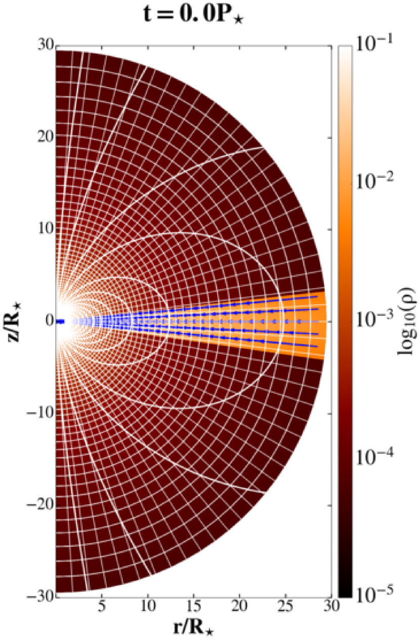
Figure 1: Initial density in the accretion disk and stellar corona in a hydrostatic equilibrium is shown in logarithmic color grading in code units, in the case with $\theta=[0,\pi]$. A sample of initial velocity vectors and stellar dipole magnetic field lines (solid lines) is shown, together with the computational grid represented with a 4x4 block of cells. In the $\theta=[0,\pi/2]$ case, initial setup is identical to the top quadrant shown here, with the addition of the symetric boundary conditions at the disk equatorial plane.

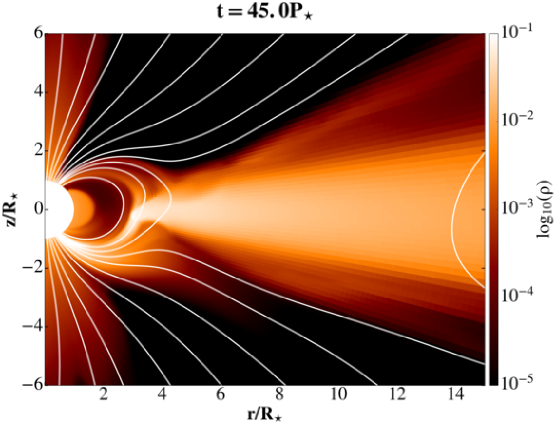
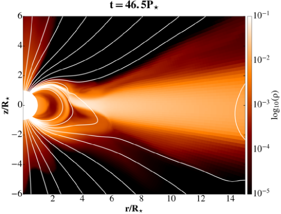
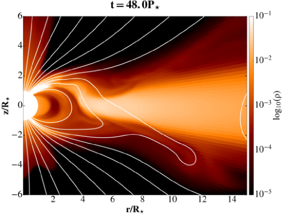
Figure 2: A sequence of snapshots from results in the case with $\theta=[0,\pi]$, in the interval when the switching of the accretion column from the southern to the northern hemisphere occurs, for which the intensities are shown in Fig. 4. Colors and lines have the same meaning as in Fig. 1.

Matter inflow onto the surface of a sufficiently magnetized star creates hot spots, as described in e.g. Ghosh & Lamb (1997), Camenzind (1990), Shu et al. (1994). Such hot spots are expected in various objects like classical T Tauri stars (Herbst et al., 1986; Johns & Basri, 1995; Alencar & Batalha, 2002), cataclysmic variables (Wickramasinghe et al., 1991; Warner, 2000), millisecond pulsars (Chakrabarty et al., 2003) and X-ray pulsars (Bildsten, 1997).

Hot spots were obtained in the pioneering series of publications on axisymmetric two-dimensional (2D) and full three-dimensional (3D) numerical simulations of star-disk interaction by M. Romanova and collaborators (Romanova et al., 2002; Long et al., 2005; Romanova et al., 2009, 2013), and in Zanni & Ferreira (2009, 2013). I confirmed the results of their 2D numerical simulations in Čemeljić et al. (2017); Čemeljić (2018).

The full 3D simulations as in Romanova et al. (2013) would still be impractical for a wide parameter study needed for a fitting of the observed light curves. Such simulations are challenging to set-up, and also demand large computational resources and time. To bridge a gap between the theoretical demands on a code, and increasingly detailed observations, I extended the axisymmetric 2D simulations from Čemeljić (2018) to a complete meridional half-plane. Using this setup, a 3D model of a star is constructed, with two identical accretion columns and hot spots positioned diametrically opposite on the stellar surface. I compute the integrated radiation flux from the surface of such a star, as observed from various angles.

The obtained intensity curve is closely related to the physical parameters in the underlying 2D axisymmetric simulation. The free parameters in the simulations are the stellar rotation rate, magnetic field strength, and the magnetic Prandtl number. Assuming the plausible dimensions of the stellar hot spots, one can find the physical parameters of the system best matching the observations. Other features, like occultation by the disk, or reprocessing of the emission in the accretion column, or use of the specific filters in the observation, could be superimposed to the presented solution.

In §2 I give a brief description of the numerical simulations set-up, followed by the results of simulations. The intensity curves in 2D are given in §3, and a 3D model constructed from them is discussed in §4. I present a case with the equatorially symmetric disk in §5 and summarize the results in §6.

2 Numerical setup and results of simulations

I performed simulations of a star-disk system magnetospheric interaction (SDMI) in a 2D-axisymmetry setup in spherical coordinates, with a logarithmically stretched grid in the radial direction, spanning 30 stellar radii, and a uniform grid in the latitudinal direction.

Set-up in the simulations which are used in the model are presented in detail in Čemeljić (2018), which closely follows Zanni & Ferreira (2009). Here is given only a brief overview of the solved equations and numerical setup. Viscous and resistive magneto-hydrodynamic equations are solved with a publicly available code pluto (v.4.1), described in Mignone et al. (2007, 2012). The solved equations are, in the cgs system of units:

$$\frac{\partial\rho}{\partial t}+\nabla\cdot(\rho{\mathbf{v}})=0$$ (1)

$$\frac{\partial\rho{\mathbf{v}}}{\partial t}+\nabla\cdot\left[\rho{\mathbf{v}}{\mathbf{v}}+\left(P+\frac{{\mathbf{B}}{\mathbf{B}}}{8\pi}\right){\mathbf{I}}-\frac{{\mathbf{B}}{\mathbf{B}}}{4\pi}-{\mathbf{\tau}}\right]=\rho{\mathbf{g}}$$ (2)

$$\frac{\partial E}{\partial t}+\nabla\cdot\left[\left(E+P+\frac{{\mathbf{B}}{\mathbf{B}}}{8\pi}\right){\mathbf{v}}-\frac{({\mathbf{v}}\cdot{\mathbf{B}}){\mathbf{B}}}{4\pi}\right]=\rho{\mathbf{g}}\cdot{\mathbf{v}}$$ (3)

$$\frac{\partial{\mathbf{B}}}{\partial t}+\nabla\times({\mathbf{B}}\times{\mathbf{v}}+\eta_{\mathrm{m}}{\mathbf{J}})=0,$$ (4)

where the symbols have have their usual meaning: $\rho$, ${\mathbf{v}}$ and P stand for the matter density, velocity and pressure. The resistivity and the viscous stress tensor are represented with $\eta_{\rm m}$ and ${\mathbf{\tau}}$, respectively. The gravity acceleration is ${\mathbf{g}}=-\nabla\Phi_{\mathbf{g}}$, with the gravitational potential of a star with mass $M_{\star}$ equal to $\Phi_{\mathbf{g}}=-GM_{\star}/R$. The electric current is given by the Ampere’s law ${\mathbf{J}}=\nabla\times{\mathbf{B}}/4\pi$ and E is the total energy density $E=P/(\gamma-1)+\rho({\mathbf{v}}\cdot{\mathbf{v}})/2+{\mathbf{B}}\cdot{\mathbf{B}}/8\pi$. The plasma polytropic index is $\gamma=5/3$.

The disk is set with the initial conditions from Kluźniak & Kita (2000), with an addition of the initially non-rotating hydrostatic corona and poloidal magnetic field, shown in Fig. 1. The first of two presented cases in the simulations is with the computational domain spanning a complete meridional half-plane $\theta=[0,\pi]$, with the resolution $R\times\theta=(217\times 200)$ grid cells. This simulation extends the previously obtained star-disk simulation results presented in Čemeljić (2018), removing the disk equatorial boundary condition-the disk mid-plane is now computed self-consistently in the computational domain. The solution with the disk equatorial plane given as a boundary condition is presented here as the second case, where the computational domain spans only a $\theta=[0,\pi/2]$ quadrant of the meridional half-plane, with the resolution $R\times\theta=(217\times 100)$ grid cells.

The viscosity and resistivity are parameterized by the Shakura & Sunyaev (1973) prescription as $\alpha_{\rm v}c^{2}/\Omega_{\rm K}$, where $\alpha_{\rm v}$ is a free parameter of viscosity, smaller than unity, and $\Omega_{\mathrm{K}}=\sqrt{GM_{\star}/r^{3}}$ is the Keplerian angular velocity at the cylindrical radius $r$. A split-field method is used, in which only changes from the initial stellar magnetic field are evolved in time (Tanaka, 1994; Powell et al., 1999). In the simulations is assumed that all the disk heating due to viscous and Ohmic dissipation is radiated away from the disk-this is why the heating and cooling terms are removed from the energy equation. Simulations are still solved in the resistive and viscous regime, because of the viscosity in the equation of motion and the resistivity in the induction equation.

After the relaxation from initial conditions, typically after a few tens of the underlying star rotations, the middle and outer part of the disk in simulations reach a quasi-stationary state, even if the accretion column still can change the point of connection to the stellar surface. The results are illustrated in Fig. 2: after t=45 stellar rotations the column is positioned at the southern hemisphere and its hot spot produces most of the emitted intensity. After one and a half rotation, at t=46.5 the column switches from the southern hemisphere to the northern. There, the new hot spot forms and its intensity is taking over as the largest contributor in the total intensity. Simultaneously, the southern hot spot intensity decreases.

Based on the 2D results, I create a 3D model to compute the intensity of radiation from hot spots, as measured by an observer at infinity, positioned at various angles with respect to the axis of rotation.

3 Intensity of radiation along the stellar rim

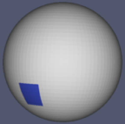
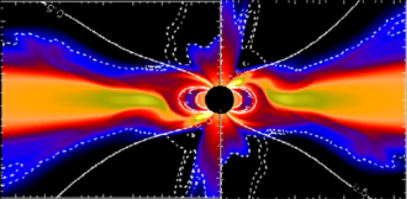
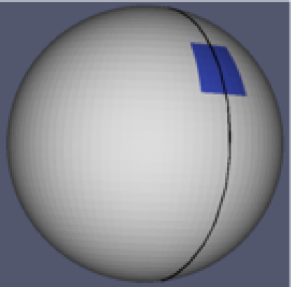
Figure 3: A composite of snapshots from the simulations in 2D, shown in the middle panel, is arranged to show the geometry of the 3D model. The color and lines meaning is the same as in Fig. 1. In the side panels are shown the corresponding hot spots atop the model sphere, rotated $\varphi=270^{\circ}$, to show the diametrically opposite hot spots atop the star.

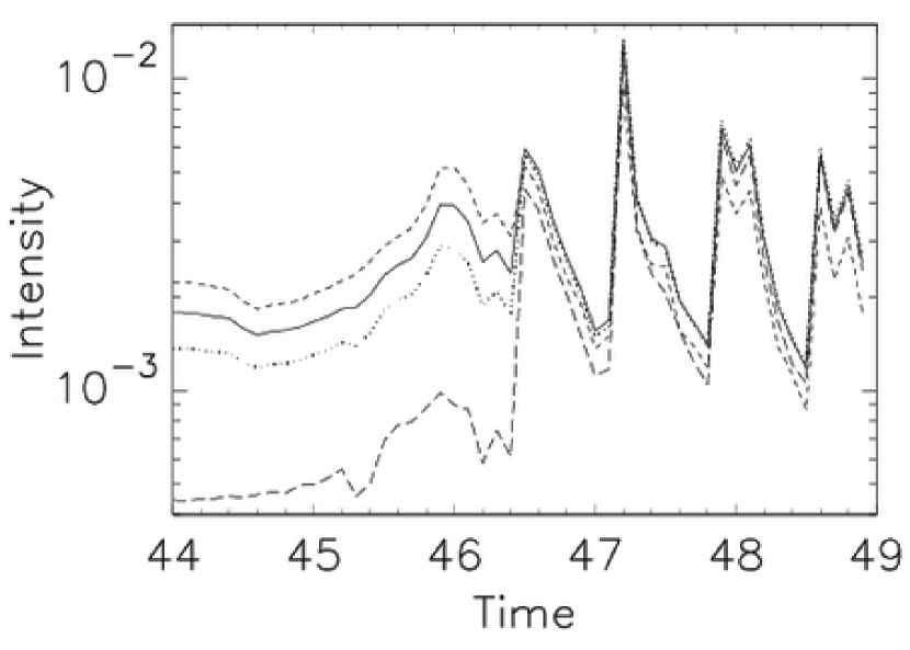
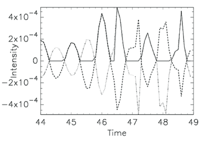
Figure 4: Intensity of emission in code units in the simulations in the $\theta=[0,\pi]$ case. Time is measured in the number of stellar rotations. Top panel: Intensity for an observer at infinity, integrated along the stellar rim, which is only one grid cell thick in the azimuthal direction. The solid, dotted, long-dashed and short-dashed lines represent the intensities for an observer positioned at a co-latitudinal angle $\alpha=$15, 30, 60 and 165 degrees, respectively. Bottom panel: Intensity in a 3D model computed from the result of the 2D simulations shown at the above panel. The dotted and dashed lines show the intensity of the modeled hot spots as seen under the angles of $15^{\circ}$ and $165^{\circ}$, respectively. The negative intensity means that the spot is not visible from a given position. The solid line shows the total intensity measured by an observer at the angle of $165^{\circ}$. A shift in phase of the observed light occurs in the time interval between 45 and 48 rotations of the star.

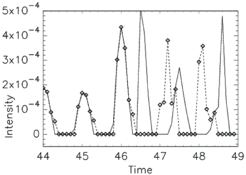
Figure 5: Intensity in the simulations in a $\theta=[0,\pi]$ case when the opposite hot spot is positioned at an angle of 180^∘ (solid line) in the antipodal case, and at 202.5^∘ (dashed line with diamond symbols) in the non-antipodal case. The intensity is computed for an observer positioned at an angle of $165^{\circ}$, measured from the north pole. The maximum of the intensity is shifted less in phase in the non-antipodal case.

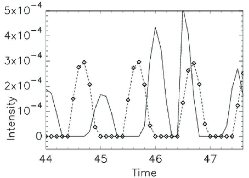
Figure 6: Illustration of the difference in the intensity curves in two simulations in a $\theta=[0,\pi]$ case with the different physical parameters. The opposite hot spot in the 3D model is positioned at an angle of 180^∘ in both cases, and the intensity is computed for an observer positioned at an angle $165^{\circ}$, measured from the north pole. The intensity from Fig. 4 in the case with $\Omega_{\star}$=$0.1\Omega_{\rm br}$, $\alpha_{\rm m}$=0.7 is repeated (solid line), along with the intensity in the case with the $\Omega_{\star}$=$0.15\Omega_{\rm br}$, $\alpha_{\rm m}$=1 (dashed line with diamond symbols). The profiles differ in both magnitude and phase.

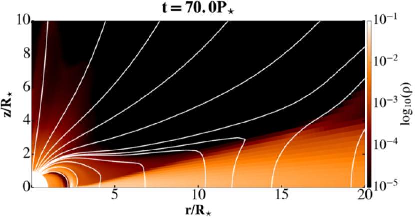
Figure 7: Zoom into a snapshot in the simulation in the $\theta=[0,\pi/2]$ case, after T=70 rotations of the central star, when the solution reached a quasi-stationary state. Lines and colors have the same meaning as in Fig. 1. The initial setup is identical to the first quadrant in the $\theta=[0,\pi]$ case, shown in Fig. 1.

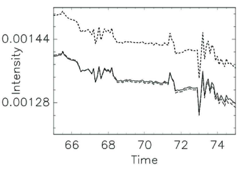
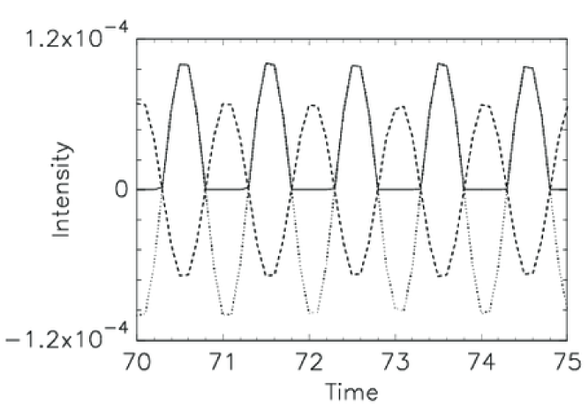
Figure 8: Intensity of emission in code units in the simulations in a $\theta=[0,\pi/2]$ case. Top Panel: Intensity for an observer at infinity, integrated along the stellar rim. The solid, short-dashed and long-dashed lines represent the intensities for an observer positioned at a co-latitudinal angle of $\alpha=$15, 30 and 60 degrees, respectively. Bottom panel: Intensity in a 3D model computed from the result shown in the above panel. The dotted and dashed lines show the intensity for the modeled hot spots as seen under the angles of $15^{\circ}$ and $165^{\circ}$, respectively. The solid line shows the total intensity measured by an observer under the angle of $165^{\circ}$. The negative intensity means that the spot is not observable from a given position.

In a 2D-axisymmetric simulation obtained is only the intensity of radiation along the line shown on the stellar surface, shown in the right panel in Fig. 3. With this information, I compute the intensity of emission from a modeled hot spot of the accretion column in the northern hemisphere. By copying the result into the opposite part of a meridional plane, I add the antipodal hot spot of the accretion column in the southern hemisphere, as shown in the left panel.

The intensity of radiation emitted along the stellar rim is

$$I_{R}=\frac{1}{\pi}\int_{\cos(\alpha-\theta)>0}F({\mathbf{R}})\cos\alpha~{}dS\ ,\mathrm{where}$$

$$F({\mathbf{R}})=\rho{\rm v}_{r}(\frac{1}{2}{\rm v}^{2}+\frac{\gamma}{\gamma-1}\frac{P}{\rho})$$

is the intensity of the radiation in the direction of the observer at infinity, positioned at the co-latitudinal angle $\alpha$ with respect to an element of the surface $dS$ - see e.g. Romanova et al. (2004). In this intensity, the stellar radiation or any obscuring effects from the disk or column is not accounted for, and the emission from the column above the stellar surface is not included.

To better illustrate the light curve modeling procedure, I choose a particular example of an uneven distribution of the intensity peaks in a 2D simulation. Such a distribution is caused by the switching of the accretion column from one stellar hemisphere to the other, shown in Fig. 2. This could help to model some of the unexplained dips, or "occultations" in the observed light curves, as in e.g. Siwak et al. (2014).

In Fig. 4, shown is a change in time in the intensity curve integrated along the stellar rim, obtained in the 2D simulation with a star rotating with 1/10 of the stellar breakup rate, viscosity and resistivity parameters equal to 1 and 0.7, respectively, and the stellar dipole magnetic field of 500 G. Time is measured in the number of stellar rotations. The observed light curve indicates that the column switched hemisphere. Before the switch, until t=46.5 the accretion column is steadily positioned in the southern hemisphere and the largest part of the emission is radiated into the portion of space with $\alpha>90^{\circ}$ (shown in the short-dashed line). After the switch of the column to the northern hemisphere, the weakening southern hot spot still contributes to the total intensity, but more of the intensity is emitted from the newly formed northern hemisphere hot spot into the $\alpha<90^{\circ}$ part of the computational domain (shown in the solid, dotted and long-dashed lines).

4 Intensity of radiation in 3D model

A hot spot in simulations is of a $\Delta\theta$ span in the latitudinal direction. To obtain a 3D model, an azimuthal extension of the hot spot is added, with the assumption that it is equal to the latitudinal one so that $\Delta\varphi=\Delta\theta$. The obtained hot spot is shaped as a part of the spherical surface shown in Fig. 3. To complete the 3D model with two antipodal accretion columns, such a hot spot is copied into a diametrically opposite hot spot on a sphere.

By rotating a model star with hot spots, the radiation intensities can be obtained for observers positioned at different angles with respect to the axis of rotation. The intensity radiated from the surface of a rotating star towards an observer positioned at the angle $\alpha$, measured from the north pole, and positioned in the plane with the zero azimuthal angle $\varphi=0$ is

$$I=\int_{\varphi}\cos\varphi d\varphi\int_{0}^{\pi}R^{2}F({\mathbf{R}})\sin\theta\cos(\alpha-\theta)d\theta\ .$$

The results of computation are shown in the bottom panel in Fig. 4. Switching of the accretion column between the stellar hemispheres is present in the modeled intensity curve as a shift of phase in the measured peaks. It follows the visibility of the hot spots because of the stellar rotation.

When analyzing the data from the observations, with a suitable set of parameters in the described model one could modify the constraints to match the observed light curve. The shape and position of the spots could be shifted in both latitude and azimuth. The azimuthal extension of each hot spot could be chosen individually.

An example of modification is a non-antipodal positioning of the opposite hot spot. In Fig. 5, with a dashed line and indicated also with the diamond symbols, is shown the intensity in a case when the opposite hot spot is positioned at an angle of 202.5^∘, instead of 180^∘. The shape of this light curve is also modified. For comparison, the intensity in the antipodal case is also shown. The maximum of the intensity is less shifted in phase after the column switches the hemisphere than in the antipodal case.

The obtained 3D model is dependent on physical parameters in the underlying 2D numerical simulation. In Fig. 6 is shown an illustration, where a shift in phase in light curve is shown between the two simulations with the different stellar rotation rates. The light curves are computed in the cases with the different resistivities in the disk, so that the obtained curves are also of the different shape and magnitude-with the solid line is repeated the intensity in the case from Fig. 4, and with the dashed line in the case with the stellar rotation rate 1/15 of the breakup rate, and the resistivity parameter $\alpha_{\rm m}$=1. The stellar magnetic field and viscosity in two simulations are the same, 500 G and $\alpha_{\rm v}$=1, respectively. In the simulation with a larger disk resistivity, there is no switch in the position of the accretion column, it remains at the northern stellar hemisphere throughout the simulation.

5 A case with equatorially symmetric disk

Simulations are often performed in only the $\theta=[0,\pi/2]$ part of the meridional plane, with an assumption of the equatorial symmetry in the disk. To create a 3D model in such cases, I repeated the simulation with the same parameters in a new domain, spanning only over the northern quadrant in the meridional plane. A snapshot in a quasi-stationary solution is shown in Fig. 7. The obtained intensity along the rim in a 2D simulation in this case is shown in the top panel in Fig. 8. It is of a similar order of magnitude as in the $\theta=[0,\pi]$ case. Since now only the intensity along a northern hemisphere part of the meridian line is obtained in the simulation, the hot spot can not switch the hemisphere. In the model, I assumed that there is no contribution to the intensity along the other, not simulated half of the latitudinal arc.

Creating a 3D model with the antipodal hot spot from this result, I obtain the intensity shown in the bottom panel in Fig. 8. Since there is no contribution from the switching of the position of the hot spot from one to the other hemisphere, there is no change in the position of the dip of the intensity curve. An observer would see the contribution to the intensity only from one hot spot at a time.

Such an intensity curve is also observed in the case when only one accretion column forms from the accretion disk onto the stellar surface. The intensity measured by an observer under the angle of $165^{\circ}$ is shown with the solid line in Fig. 8.

6 Summary

I compute the intensity of emission from a hot spot created by the accretion column infalling onto a stellar surface in the numerical simulations of star-disk magnetospheric interaction. From the results of 2D simulations, with minimal additional assumptions is computed a full 3D model.

In a descriptive example, I show how a shift in phase of the intensity peaks can be explained by switching of the accretion column from one stellar hemisphere to the other. The obtained intensity is closely related to the geometrical and physical parameters of the underlying star-disk numerical simulation.

One case of a difference in results with modification of the geometry in 3D model is illustrated in an example, in which the opposite hot spot on the stellar surface is not placed exactly in the antipodal position. The shape and phase of the intensity maximum change.

To further illustrate the versatility of the model, I compare the modeled intensity curves with a modification in the physical parameters in the underlying numerical simulation. Both the shape and phase of the resulting intensity curves in the full 3D model are modified with such a change. I also show the results in the cases when a hot spot does not switch the stellar hemisphere, or when there is only one accretion column hot spot at the stellar surface.

In the presented models, assumed are hot spots of the same shape and area. With the appropriate modifications, intensity from hot spots of different extensions can be computed. With an addition of the observational filter responses and occultation patterns with the disk and column, the model could account for the different geometries of the system and the effects of a medium through which the radiation passes on the way to an observer.

References

- Alencar & Batalha (2002) Alencar, S.H.P., & Batalha, C., 2002, ApJ, 571, 378
- Bildsten (1997) Bildsten, L., et al., 1997, ApJS, 113, 367
- Camenzind (1990) Camenzind, M., 1990, Rev. Mod. Astron., 3, 234
- Čemeljić et al. (2017) Čemeljić, M., Parthasarathy, V. & Kluźniak, W., 2017, JPhCS, 932, 012028
- Čemeljić (2018) Čemeljić, M., 2018, arXiv:1811.02808, submitted to A&A
- Chakrabarty et al. (2003) Chakrabarty, D., Morgan, E.H., Muno, M.P., Galloway, D.K., Wijnands, R., Van Der Klis, M., & Markwardt, G.B., 2003, Nature, 424, 42
- Ghosh & Lamb (1997) Ghosh, P., & Lamb, F.K., 1997, ApJ, 234, 296
- Herbst et al. (1986) Herbst, W., et al., 1986, ApJ, 310, L71
- Johns & Basri (1995) Johns, C.M., & Basri, G., 1995, ApJ, 449, 341
- Kluźniak & Kita (2000) Kluźniak, W., Kita, D., 2000, arXiv:astro-ph/0006266
- Mignone et al. (2007) Mignone, A., Bodo, G., Massaglia, S., Matsakos T., Tesileanu O., Zanni C., Ferrari A., 2007, ApJS, 170, 228
- Mignone et al. (2012) Mignone, A., Zanni, C., Tzeferacos, P., van Straalen, B., Colella, P., and Bodo, G., 2012, ApJS, 198, 7
- Powell et al. (1999) Powell, K. G., Roe, P. L., Linde, T. J., Gombosi, T. I., & De Zeeuw, D. L. 1999, J. Comput. Phys, 154, 284
- Romanova et al. (2002) Romanova, M.M., Ustyugova, G.V., Koldoba, A.V., Lovelace, R.V.E., 2002, ApJ, 578, 420
- Romanova et al. (2004) Romanova, M.M., Ustyugova, G.V., Koldoba, A.V., Lovelace, R.V.E., 2004, ApJ, 610, 920
- Long et al. (2005) Long, M., Romanova, M.M., & Lovelace, R.V.E., 2005, ApJ, 634, 1214
- Romanova et al. (2009) Romanova, M.M., Ustyugova, G.V., Koldoba, A.V., Lovelace, R.V.E., 2009, MNRAS, 399, 1802
- Romanova et al. (2013) Romanova, M.M., Ustyugova, G.V., Koldoba, A.V., Lovelace, R.V.E., 2013, MNRAS, 430, 699
- Shakura & Sunyaev (1973) Shakura, N.I., Sunyaev, R.A., 1973, A&A, 24, 337
- Shu et al. (1994) Shu, F.H., Najita, J., Ostriker, E.C., Wilkin, F., Ruden, S.P., & Lizano, S., 1994, ApJ, 429, 781
- Siwak et al. (2014) Siwak, M., Rucinski, S.M., Matthews, J.M., Guenther, D.B., Kuschnig, R., Moffat, A.F.J., Rowe, J.F., Sasselov, D., Weiss, W.W., 2014, MNRAS, 444, 327
- Tanaka (1994) Tanaka, T. 1994, J. Comput. Phys., 111, 381
- Warner (2000) Warner, B., 2000, PASP, 112, 1523
- Wickramasinghe et al. (1991) Wickramasinghe, D.T., Wu, K. & Ferrario, L., 1991, MNRAS, 249, 460
- Zanni & Ferreira (2009) Zanni, C., Ferreira, J., 2009, A&A, 512, 1117
- Zanni & Ferreira (2013) Zanni, C., Ferreira, J., 2013, A&A, 550, A99