Can the complex Langevin method see the deconfinement phase transition in QCD at finite density?

Abstract:

Exploring the phase diagram of QCD at finite density is a challenging problem since first-principle calculations based on standard Monte Carlo methods suffer from the sign problem. As a promising approach to this issue, the complex Langevin method (CLM) has been pursued intensively. In this work, we investigate the applicability of the CLM in the vicinity of the deconfinement phase transition using the four-flavor staggered fermions. In particular, we look for a signal of the expected first order phase transition within the validity region of the CLM.

1 Introduction

Exploring the phase diagram of QCD at finite density and temperature is important due to its relevance to the heavy-ion collision physics and the determination of the equation of state for neutron stars. However, lattice QCD simulations based on conventional Monte Carlo algorithms suffer from a severe sign problem in the finite density region.

To overcome this problem, the complex Langevin method (CLM) [1, 2] has been investigated intensively in recent years. Basically, it is an extension of the stochastic quantization to theories with a complex action. In this framework, the expectation value of holomorphic observables is computed by solving the complex Langevin equation, which describes the stochastic time-evolution of the complexified dynamical variables. This procedure does not rely on the probabilistic interpretation of the Boltzmann weight $e^{-S}$, and hence it is free from the sign problem. However, the equivalence to the familiar path integral quantization does not always hold [3, 4] unlike the case with a real action. Recently, a necessary and sufficient condition for the equivalence based on the probability distribution of the drift term has been proposed [5]; i.e., the CLM gives correct results if and only if the probability distribution of the drift term decays exponentially or faster. Because of this condition, the CLM works in some parameter region of finite density QCD, but not in the entire region. As we will see in the following, the distribution falls off with a power law in some region, which implies that the CLM is no longer valid there. Since one can easily monitor the distribution while generating configurations, it is useful and preferable to judge the validity of the CLM in this way in actual simulations for each set of parameters.

In this paper we discuss the applicability of the CLM in the vicinity of the deconfinement transition with $N_{\rm f}=4$ staggered fermions at finite temperature $T$ and finite chemical potential $\mu$. This transition is known to be of first order at $\mu=0$ [6], and it is expected to be so also at $\mu\neq 0$ based on the canonical ensemble method [7, 8]. Recently the CLM and the standard reweighting method have been applied to this theory for comparison [9]. While the deconfinement transition was accessible by the reweighting method unless $\mu$ or the lattice size is not too large, it turned out to be difficult to access by the CLM for the chosen setup because the simulation becomes unstable for small $\beta$. Motivated by this result, we perform simulations with larger lattice size in the temporal direction so that the phase transition occurs at larger $\beta$, and investigate whether the CLM has an ability to probe the deconfinement transition in different setups.

The rest of this article is organized as follows. In section 2 we give a brief overview on the application of the CLM to lattice QCD at finite density. In section 3 we present our results. Section 4 is devoted to a summary and discussions.

2 Complex Langevin method for finite density QCD

We apply the CLM to lattice QCD on a four-dimensional lattice with the temporal extent $N_{\rm t}$ and the spatial extent $N_{\rm s}$. Throughout this paper, we set the lattice spacing to unity. The partition function is given by

$$Z=\int\prod_{x\nu}dU_{x\nu}\,\mathrm{det}M(U;\mu)\,e^{-S_{\rm g}(U)}\ ,$$ (1)

where $U_{x\nu}\in\mathrm{SU}(3)$ ($\nu=1,2,3,4$) are the link variables with $x=(x_{1},x_{2},x_{3},x_{4})$ being the coordinates of each site. For the gauge action $S_{\rm g}(U)$, we use the Wilson plaquette action defined by

$$S_{\rm g}=-\frac{\beta}{6}\sum_{x}\sum_{\mu<\nu}\mathrm{tr}\Big{(}U_{x,\mu\nu}+U_{x,\mu\nu}^{-1}\Big{)}\ ,\quad\quad U_{x,\mu\nu}=U_{x\mu}U_{x+\hat{\mu},\nu}U_{x+\hat{\nu},\mu}^{-1}U_{x\nu}^{-1}\ ,$$ (2)

where $\hat{\mu}$ is the unit vector in the $\mu$ direction. For fermions, we use the $N_{\rm f}=4$ unimproved staggered fermion with the degenerate quark mass $m$, which corresponds to choosing the fermion matrix $M(U;\mu)$ in (1) as

$$M(U;\mu)_{xy}=m\delta_{xy}+\sum_{\nu=1}^{4}\frac{\eta_{\nu}(x)}{2}\left(e^{\mu\delta_{\nu 4}}U_{x\nu}\delta_{x+\hat{\nu},y}-e^{-\mu\delta_{\nu 4}}U_{x-\hat{\nu},\nu}^{-1}\delta_{x-\hat{\nu},y}\right)\ ,$$ (3)

where $\mu$ represents the quark chemical potential and $\eta_{\nu}(x)=(-1)^{x_{1}+\cdots+x_{\nu-1}}$ is a site-dependent sign factor. The sign problem is caused by the fermion determinant $\mathrm{det}M(U;\mu)$ appearing in (1). We impose anti-periodic boundary conditions for the fermionic field in the temporal direction. The temperature is then given by $T=1/N_{\rm t}$.

The CLM is one of the most promising approaches to overcome the sign problem. In this method, the link variables $U_{x\mu}$ defined as $\mathrm{SU}(3)$ matrices are complexified into $\mathrm{SL}(3,\mathbb{C})$ matrices, which we denote as $\mathcal{U}_{x\mu}$. Then we consider a fictitious time evolution of the complexified variables given by the complex Langevin equation with stepsize $\epsilon$

$$\mathcal{U}_{x\mu}(t+\epsilon)=\exp\left(i\sum_{a=1}^{8}\lambda_{a}\left[-\epsilon v_{ax\mu}(\mathcal{U}(t))+\sqrt{\epsilon}\eta_{ax\mu}(t)\right]\right)\ \mathcal{U}_{x\mu}(t)\ ,$$ (4)

where $\lambda_{a}\ (a=1,\cdots,8)$ are the SU(3) generators normalized by $\mathrm{tr}(\lambda_{a}\lambda_{b})=\delta_{ab}$. The noise term $\eta_{ax\mu}(t)$ is composed of real gaussian random numbers normalized as

$$\langle\eta_{ax\mu}(s)\eta_{by\nu}(t)\rangle=2\delta_{ab}\delta_{xy}\delta_{\mu\nu}\delta_{st}\ .$$ (5)

The drift term $v_{ax\mu}(\mathcal{U}(t))$ is defined by the holomorphic extension of

$$v_{ax\mu}(U)=\left.\frac{d}{d\alpha}S(e^{i\alpha\lambda_{a}}U_{x\mu})\right|_{\alpha=0}$$ (6)

defined for the SU(3) link variables with the total action $S[U]=S_{\rm g}[U]-\log\det M(U;\mu)$.

A subtle point of the CLM is that it is not guaranteed to yield correct results, and hence one has to check the reliability of the results after generating configurations. According to the criterion proposed in ref. [5], the CLM is equivalent to the usual path integral formulation if the probability distribution of the drift term shows an exponential fall-off. In the case of finite density QCD, we define the magnitude of the drift term by

$$v=\max_{x,\mu}\sqrt{\frac{1}{3}\sum_{a=1}^{8}|v_{ax\mu}(\mathcal{U})|^{2}}\ .$$ (7)

There are actually two cases in which the above criterion is violated. One is the singular drift problem [10, 11], which occurs because of the appearance of the inverse $M^{-1}$ in the drift term when the fermion matrix $M(\mathcal{U};\mu)$ has near-zero eigenvalues. In order to detect this problem, we probe the contributions to the drift term from the fermion determinant $\det M(\mathcal{U};\mu)$.

The other case which leads to the violation of the criterion is the excursion problem [3, 4], which occurs when the complexified link variables become too far from unitary matrices. In order to detect this problem, it is useful to probe the unitarity norm defined by

$${\cal N}=\frac{1}{12N_{\rm V}}\sum_{x\mu}\mathrm{tr}\left(\mathcal{U}_{x\mu}\mathcal{U}_{x\mu}^{\dagger}-{\bf 1}\right)\ ,$$ (8)

which measures the deviation of the complexified link variables from SU(3). Here we defined $N_{\rm V}=N_{\rm t}N_{\rm s}^{3}$, which represents the volume of the four-dimensional Euclidean space.

As important observables, we consider the Polyakov loop, which is defined by

$$P =\frac{1}{3N_{\rm s}^{3}}\sum_{\vec{x}}\mathrm{tr}\Big{(}U_{(\vec{x},1),4}U_{(\vec{x},2),4}\dots U_{(\vec{x},N_{t}),4}\Big{)}\ ,$$ (9)

where $\vec{x}=(x_{1},x_{2},x_{3})$, and the baryon number density defined by

$$n =\frac{1}{3N_{\rm V}}\frac{\partial}{\partial\mu}\log Z=\frac{1}{3N_{\rm V}}\left\langle\sum_{x}\frac{\eta_{4}(x)}{2}\mathrm{tr}\Big{(}e^{\mu}M^{-1}_{x+\hat{4},x}U_{x4}+e^{-\mu}M^{-1}_{x-\hat{4},x}U_{x-\hat{4},4}^{-1}\Big{)}\right\rangle\ .$$ (10)

3 Results

In the previous work [9], the validity range of the CLM was discussed with the maximum lattice size being $16^{3}\times 8$. There it was found for $\mu/T=0.96$ with the quark mass $m=0.01$, for instance, that the CLM breaks down at $\beta\sim 5.15$, which prevented the authors from reaching the transition point, which is slightly below $5.15$. Based on this result, we employ a lattice with larger temporal size $N_{\rm t}=12$, which is expected to shift the transition point to larger $\beta$, hoping that the CLM can see the phase transition within the region of validity. The quark chemical potential is chosen as $\mu=0.1$, which corresponds to $\mu/T=1.2$. We use an adaptive stepsize [12] with the initial value $\epsilon=5\times 10^{-5}$ and perform the gauge cooling [13] (See refs. [14, 5] for its justification) to minimize the unitarity norm ${\cal N}$ at each Langevin step.

3.1 $\beta$-dependence at $m=0.01$

Here we show our results obtained at $m=0.01$ for $5.2\leq\beta\leq 5.6$ on a $20^{3}\times 12$ lattice. First we check the reliability of the CLM. In Fig. 1 we plot the probability distribution of the fermionic drift term and the history of the unitarity norm. At $\beta=5.2$ and 5.3, we observe that the distribution of the drift term falls off with a power law and the unitarity norm grows rapidly with the Langevin time. Therefore, we conclude that the CLM is not reliable for these values of $\beta$.

In order to probe the deconfinement transition, we measure the Polyakov loop and the baryon number density. In Fig. 2 we plot the expectation values of these quantities as a function of $\beta$. Focusing on the reliable data at $\beta\geq 5.4$, we find that both of them decrease gradually as $\beta$ is lowered, but they remain significantly away from zero suggesting that the system is in the deconfined phase. The first order phase transition seems to be hidden in the unreliable region, which is similar to the situation in ref. [9]. Thus, we find that increasing the temporal size of the lattice does not enable us to see the deconfinement phase transition.

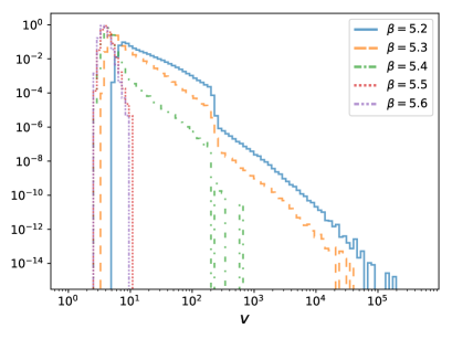
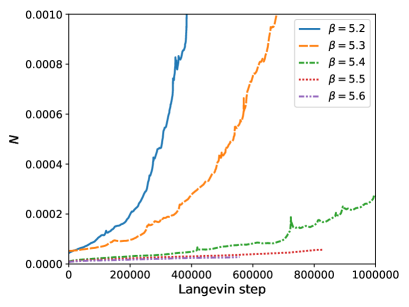
Figure 1: The histogram of the fermionic drift term (Left) and the history of the unitarity norm (Right) are plotted for various $5.2\leq\beta\leq 5.6$ with $m=0.01$ on a $20^{3}\times 12$ lattice.

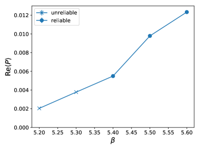
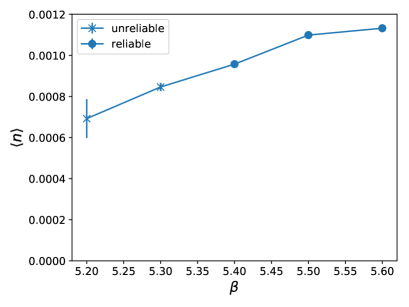
Figure 2: The real part of the Polyakov loop (Left) and the baryon number density (Right) are plotted against $\beta$ for $m=0.01$ on a $20^{3}\times 12$ lattice. Circles and crosses represent reliable data and unreliable data, respectively.

3.2 Increasing the quark mass

From Figs. 10 and 11 of ref. [9], we find that the critical $\beta$ can be shifted to larger values also by increasing the quark mass, which provides us with another possibility to observe the phase transition by the CLM. Below we show our results obtained at $0.01\leq m\leq 0.5$ with fixed $\beta=5.4$ on a $24^{3}\times 12$ lattice.

In Fig. 3 we show the probability distribution of the drift term and the history of the unitarity norm. At $m\geq 0.2$, we find that the distribution of the fermionic drift term falls off with a power law and the unitarity norm grows rapidly, which implies that the CLM is not reliable there.

In Fig. 4 we show the expectation value of the Polyakov loop and the baryon number density as a function of the quark mass. Focusing on the reliable data at $m\leq 0.1$, we find that both of them decrease with increasing $m$, but they remain significantly nonzero suggesting that the system is in the deconfined phase. However, the sharp drop of the baryon number density at $m\sim 0.1$ suggests that the system enters the confined phase slightly above that point. Thus we find that the first order phase transition is hidden in the unreliable region here as well.

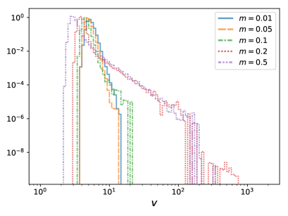
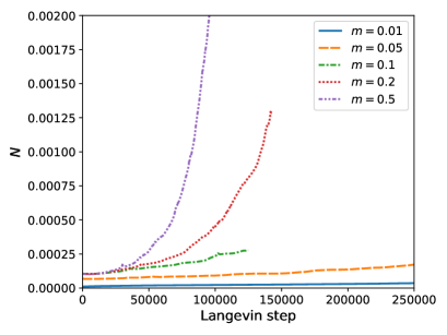
Figure 3: The histogram of the fermionic drift term (Left) and the history of the unitarity norm (Right) are plotted for various $0.01\leq m\leq 0.5$ with $\beta=5.4$ on a $24^{3}\times 12$ lattice.

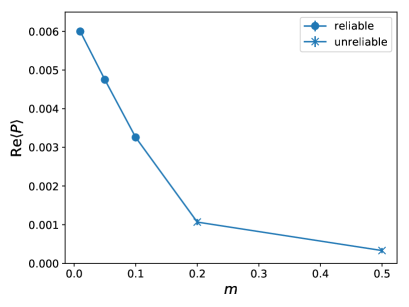
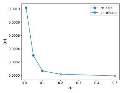
Figure 4: The real part of the Polyakov loop (Left) and the baryon number density (Right) are plotted against the quark mass $m$ for $\beta=5.4$ on a $24^{3}\times 12$ lattice. Circles and crosses represent reliable data and unreliable data, respectively.

4 Summary and outlook

In this paper we have investigated the validity region of the CLM for lattice QCD at finite chemical potential using the criterion based on the probability distribution of the drift term. In particular, we have discussed whether the CLM has an ability to probe the deconfinement transition. We have performed lattice QCD simulations with four-flavor staggered fermions on lattices with larger temporal size $N_{\rm t}=12$ than the previous study with $N_{\rm t}=4,6,8$ so that the critical $\beta$ is shifted to a larger value. The chemical potential is set to $\mu=0.1$, which corresponds to $\mu/T=1.2$. Our results obtained at $m=0.01$ on a $20^{3}\times 12$ lattice suggest that the singular drift problem occurs at sufficiently small $\beta$, which seems to hide the phase transition. As another possibility, we have also increased $m$ at fixed $\beta=5.4$ on a $24^{3}\times 12$ lattice, which showed that the singular drift problem occurs before the phase transition is observed. When the singular drift problem occurs, the unitarity norm shows a rapid growth at the same time. From these results, we speculate that the singular drift problem occurs in the confined phase quite generally unless the quark mass becomes very large. It would be interesting to see whether the CLM remains applicable in the deconfined phase even at larger $\mu$ and lower $T$. Simulations in this direction are underway.

References

- [1] G. Parisi, Phys. Lett. B131, 393 (1983).
- [2] J. R. Klauder, Phys. Rev. A29, 2036 (1984).
- [3] G. Aarts, E. Seiler, and I.-O. Stamatescu, Phys. Rev. D81, 054508 (2010), arXiv:0912.3360.
- [4] G. Aarts, F. A. James, E. Seiler, and I.-O. Stamatescu, Eur. Phys. J. C71, 1756 (2011), arXiv:1101.3270.
- [5] K. Nagata, J. Nishimura, and S. Shimasaki, Phys. Rev. D94, 114515 (2016), arXiv:1606.07627.
- [6] M. Fukugita, H. Mino, M. Okawa, and A. Ukawa, Phys. Rev. Lett. 65, 816 (1990).
- [7] P. de Forcrand and S. Kratochvila, Nucl. Phys. Proc. Suppl. 153, 62 (2006), arXiv:hep-lat/0602024.
- [8] A. Li, A. Alexandru, K.-F. Liu, and X. Meng, Phys. Rev. D82, 054502 (2010), arXiv:1005.4158.
- [9] Z. Fodor, S. D. Katz, D. Sexty, and C. Torok, Phys. Rev. D92, 094516 (2015), arXiv:1508.05260.
- [10] A. Mollgaard and K. Splittorff, Phys. Rev. D88, 116007 (2013), arXiv:1309.4335.
- [11] J. Nishimura and S. Shimasaki, Phys. Rev. D92, 011501 (2015), arXiv:1504.08359.
- [12] G. Aarts, F. A. James, E. Seiler, and I.-O. Stamatescu, Phys. Lett. B687, 154 (2010), arXiv:0912.0617.
- [13] E. Seiler, D. Sexty, and I.-O. Stamatescu, Phys. Lett. B723, 213 (2013), arXiv:1211.3709.
- [14] K. Nagata, J. Nishimura, and S. Shimasaki, PTEP 2016, 013B01 (2016), arXiv:1508.02377.
- [15] K. Nagata, J. Nishimura, and S. Shimasaki, (2018), arXiv:1805.03964.