On the physisorption of water on graphene: Sub-chemical accuracy from many-body electronic structure methods

Abstract

Molecular adsorption on surfaces plays a central role in catalysis, corrosion, desalination, and many other processes of relevance to industry and the natural world. Few adsorption systems are more ubiquitous or of more widespread importance than those involving water and carbon, and for a molecular level understanding of such interfaces water monomer adsorption on graphene is a fundamental and representative system. This system is particularly interesting as it calls for an accurate treatment of electron correlation effects, as well as posing a practical challenge to experiments. Here, we employ many-body electronic structure methodologies that can be rigorously converged and thus provide faithful references for the molecule-surface interaction. In particular, we use diffusion Monte-Carlo (DMC), coupled cluster (CCSD(T)), as well as the random phase approximation (RPA) to calculate the strength of the interaction between water and an extended graphene surface. We establish excellent, sub-chemical, agreement between the complementary high-level methodologies, and an adsorption energy estimate in the most stable configuration of approximately -100 meV is obtained. We also find that the adsorption energy is rather insensitive to the orientation of the water molecule on the surface, despite different binding motifs involving qualitatively different interfacial charge reorganisation. In producing the first demonstrably accurate adsorption energies for water on graphene this work also resolves discrepancies amongst previously reported values for this widely studied system. It also paves the way for more accurate and reliable studies of liquid water at carbon interfaces with cheaper computational methods, such as density functional theory and classical potentials.

Subject area: Chemical Physics

Keywords: graphene, water adsorption, quantum Monte-Carlo, coupled cluster theory, random phase approximation, density functional theory

I Introduction

The adsorption and diffusion of molecules on surfaces is central to countless industrial applications, including catalysis, gas storage, desalination, and more. Of all the many and varied molecular adsorption systems, few, if any, are of greater importance than those involving water and carbon. Such interfaces are, for example, at the very heart of water purification and desalination membranes. In addition, water-carbon interfaces are incredibly interesting scientifically in that they can exhibit unique and fascinating behavior Fumagalli et al. (2018); Abraham et al. (2017); Joshi et al. (2014); Nair et al. (2012); Algara-Siller et al. (2015); Secchi et al. (2016); Radha et al. (2016); Siria et al. (2017); Yoshida et al. (2018). For example, water can flow in an essentially frictionless manner across the surfaces of sp²-bonded carbon materials (both carbon nanotubes and graphene) Hummer et al. (2001); Strogatz et al. (2005); Holt (2006); Secchi et al. (2016). However, seemingly similar materials such as nanotubes made from hexagonal boron nitride do not exhibit such behaviour Secchi et al. (2016); Radha et al. (2016); Tocci et al. (2014); Michaelides (2016); Esfandiar et al. (2017).

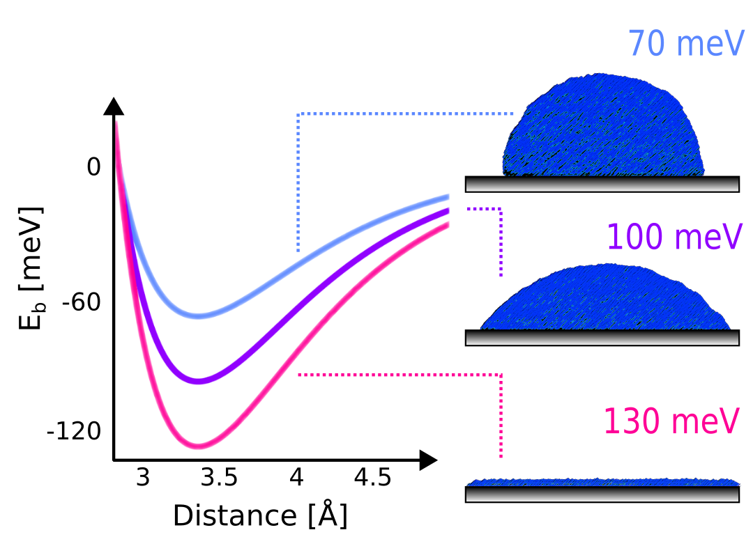
Figure 1: Water droplet modeled by a coarse-gained water model (mW) and Morse-type water-wall potential with varying adsorption strengths (see appendix A). This figure illustrates that modest changes in the adsorption energy lead to drastic changes in the wetting properties of the surface.

Apart from water purification, wetting of surfaces is of general interest and graphene can be seen as representative van der Waals (vdW) material. Many of these exciting experiments showing exceptional properties of water on graphitic surfaces and the outstanding applications lack a full molecular level understanding of the processes and the mechanisms involved. In order to gain further insight, it is necessary to complement experimental investigations with theoretical approaches. The most fundamental property of any adsorption system is the question of the adsorption bond itself, what the strength of the interaction is, the orientation of the molecule, and the physical nature of the interaction. For water-carbon interfaces at their simplest level, this comes down to understanding how a single water molecule bonds to a single sheet of graphene. Accurately establishing the strength of this interaction is important because it directly impacts upon the behavior of water at graphitic surfaces. For instance, as illustrated in Fig. 1, molecular dynamics simulations (see appendix A) reveal that altering the strength of the water-graphene interaction by as little as 60 meV transforms the graphene surface from hydrophobic to hydrophilic.

Experimentally, water molecules readily form clusters on surfaces and graphene is no exception Björneholm et al. (2016).This has so far prohibited single molecule adsorption measurements of water on graphene. On the other hand, the subtle balance of the contributing intermolecular interactions and the very high accuracy required makes the theoretical description by electronic structure methods challenging. Indeed, adsorption energy estimates have to be more accurate than so called “chemical accuracy”, which is defined as 1 kcal/mol or 43 meV, in order to be useful in this system. This is often beyond the accuracy delivered by density functional theory (DFT); the most widely used electronic structure method for understanding molecules at surfaces. Indeed, previous work has shown that DFT can provide any value for the water adsorption strength on graphene between 0 and -160 meV depending on the exchange-correlation functional and vdW-correction Ma et al. (2011); Hamada (2012); Silvestrelli and Ambrosetti (2014); Lorenz et al. .

Table 1: Equilibrium adsorption energies $E_{\text{ad}}$ in meV of a single water monomer (in the so-called “2-leg” configuration; see Fig. 2) on graphene as estimated from various electronic structure methods. A brief comment is also made about each adsorption energy estimate.

$E_{\text{ad}}$/meV	Method	Comment
-130	DFT/CC Rubeš et al. (2009)	Corrects DFT based on differences on small clusters
-130	DFT-SAPT Jenness et al. (2010)	Extrapolation from cluster
-70 $\pm$ 10	DMC Ma et al. (2011)	Periodic system, large stochastic error, finite-size effects
-135	i-CCSD(T) Voloshina et al. (2011)	Incremental expansion, correlation from cluster, small basis set
-87	p-CCSD(T)	Periodic system, finite-size corrected
-99 $\pm$ 6	DMC	Periodic system, finite-size corrected

The variation in adsorption energies obtained from DFT calls for many-body methodologies that can be rigorously converged. The application of such methods to extended (periodic) surfaces, however, does not come without significant challenges Michaelides et al. (2015). Table 1 summarizes attempts to provide benchmark quality binding energies for water on graphene with state-of-the-art electronic structure methods  Rubeš et al. (2009); Jenness et al. (2010); Ma et al. (2011); Voloshina et al. (2011); Feller and Jordan (2000). It can be seen that the previous estimates range from about 70 to about 130 meV. Whilst this is narrower than the range obtained from DFT, the deviations are clearly too high to make faithful predictions on the water-graphene interactions. Although these previous attempts have involved great care and considerable effort, they all have possible weaknesses and potential shortcomings. Here, in light of a new estimate of the adsorption energy of water on graphene, we will critically examine previous estimates and in so-doing resolve the discrepancies between previous reports. Our new study relies on impressive progress with state-of-the-art electronic structure methods and their implementation in scaleable software suits in the past few years. These developments together with an increased capacity of available computational resources makes the accurate determination of binding energies on extended surfaces feasible. It is thus timely to analyze the physisorption of water on graphene again and in so-doing we are able to demonstrate that different many-body electronic structure methods indeed agree within sub-chemical accuracy.

In the remainder of this manuscript we briefly discuss the water monomer binding motifs considered and summarize the main methodologies employed (Section II). In Section III, we summarize and discuss our best estimates for the adsorption energies (III.1) of water on a periodic free-standing graphene sheet and on small sp²-bonded molecular analogues of graphene (specifically benzene and coronene). Following this we discuss the discrepancies between previous literature values (III.2), the implications of our revised adsorption energies including an assessment of the performance of certain DFT functionals (III.3), and analyze the physical nature of the adsorption bond (IV). Conclusions and a future perspective are given in section V.

II Methods

Various computational approaches have been used in the current study. Here, mainly for orientation purposes, we briefly comment on the structures examined, the quantities computed, and the main methods used. Full details of all methods are provided in Appendix B.

Water monomer adsorption was considered in three different motifs, dubbed 0-leg, 1-leg, and 2-leg as defined in Fig. 2. These are the most widely discussed adsorption structures in previous studies Rubeš et al. (2009); Jenness et al. (2010); Ma et al. (2011); Voloshina et al. (2011); Feller and Jordan (2000). The adsorption energy $E_{\text{ad}}$ is the minimum, obtained at the equilibrium distance $d_{\text{ad}}$, of the binding curve:

$$E_{\text{b}}(d)=E_{\text{W+G}}(d)-E_{\text{W+G}}(d_{\text{far}})\,,$$ (1)

where $E_{\text{W+G}}(d)$ is the energy of the system with the water at a distance $d$ from the graphene sheet, and $E_{\text{W+G}}(d_{\text{far}})$ is the energy of the non-interaction system, with water far away at a distance $d_{\text{far}}$ from graphene . Note that what is computed here is the static electronic energy without inclusion of thermal or nuclear quantum effects.

One of the key techniques used in this study is diffusion Monte-Carlo (DMC) Foulkes et al. (2001). DMC can be readily applied to periodic systems and in the past few years the computational efficiency and accuracy of the technique has improved significantly. In particular, a recent algorithmic development has reduced computational effort by up to two orders of magnitude Zen et al. (2016a). Subsequently it was shown that the new DMC algorithm together with an effective estimation of finite-size errors yields chemically accurate lattice energies for a range of molecular crystals (including ice and delocalized $\pi$-systems) with modest computational cost Zen et al. (2018). In the current study we performed DMC studies with the CASINO code Needs et al. (2010) for water on benzene, coronene, and graphene in periodic unit cells. For adsorption on graphene a large 5$\times$5 unit cell was employed.

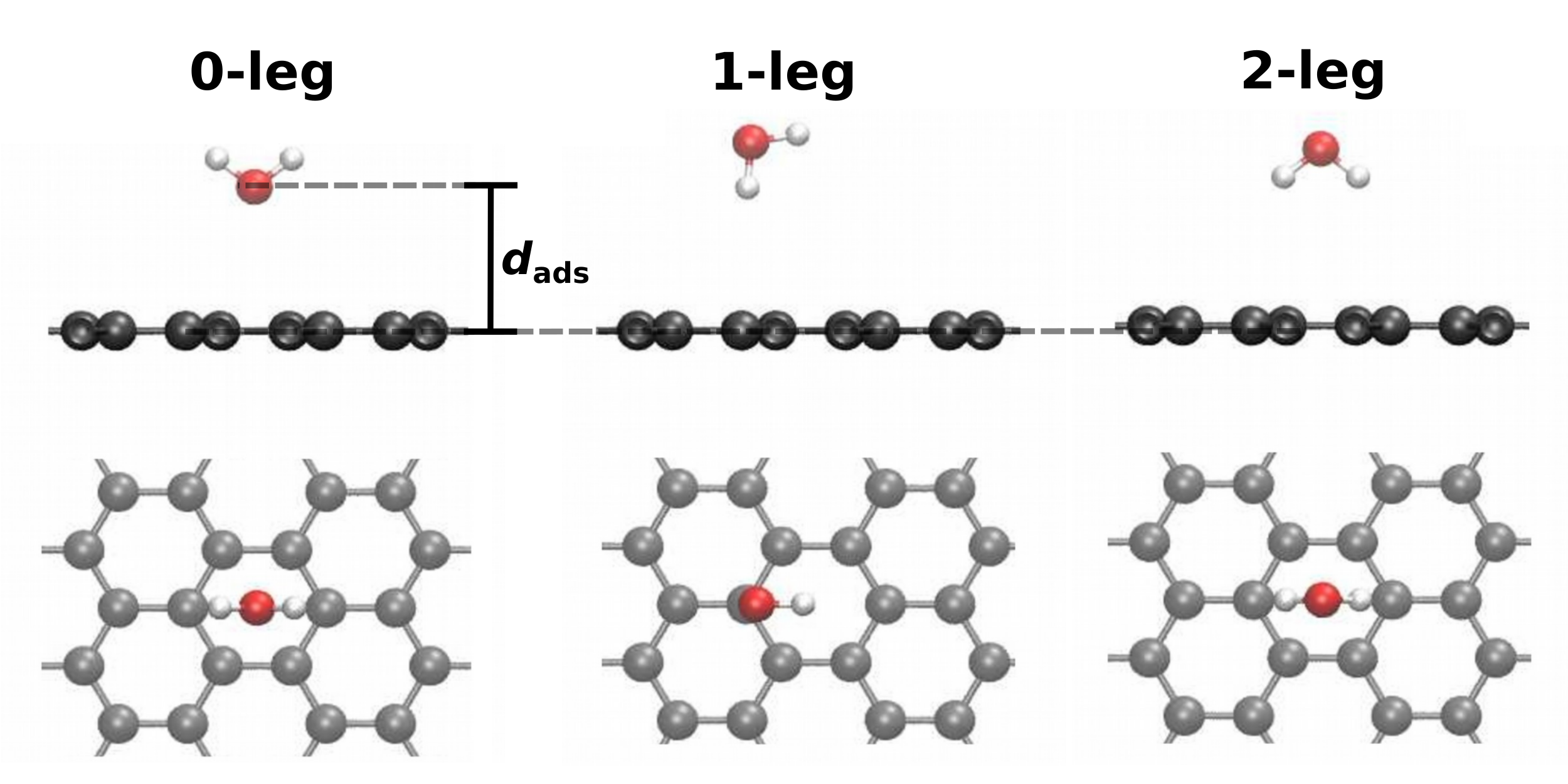
Figure 2: Water adsorption structures considered. We show the 0-leg, 1-leg, and 2-leg motif each from the side (top) and from above (bottom). The distance $d$ is defined by the distance of the oxygen atom from the graphene plane. A periodic 5$\times$5 graphene cell is used in most calculations, while for clarity only a small part of the simulation cell is shown. All equilibrium geometries are provided as supporting information.

The second many-body approach used in this study is coupled cluster, for both water adsorption on benzene and coronone and on periodic graphene. Specifically, we used linear scaling domain based pair natural orbital coupled cluster including singles, doubles, and perturbative triples [denoted here as the L-CCSD(T) method Riplinger et al. (2013)], as implemented in the ORCA program package Neese (2012) for the finite sized cluster models. Periodic coupled cluster including singles, doubles, and perturbative triples [denoted here as the p-CCSD(T)] was used for adsorption on graphene Booth et al. (2013). For these calculations a periodic 4$\times$4 unit cell was employed and the coupled cluster code CC4S interfaced to the VASP code Kresse and Furthmüller (1996a, b) was used Hummel et al. (2017); Gruber et al. (2018).

The third many-body approach employed is the random phase approximation (RPA) Nozières and Pines (1958); Harl and Kresse (2008, 2009); Eshuis et al. (2012); Wilhelm et al. (2016), which computes the correlation energy based on the electron density response function. RPA is computationally more affordable than CCSD(T) and has recently shown good results, in particular if singles corrections are introduced Schimka et al. (2010); Ren et al. (2011); Klimeš (2016); Zen et al. (2018). However, it includes fewer excitation types than CCSD(T) and thus one has to carefully test it’s accuracy. Here we used RPA based on PBE orbitals, i.e. the exact exchange energy EXX@PBE combined with the correlation RPA@PBE. In addition, the contribution from GW single excitations (GWSEs) was computed based on the work of Klimeš et al. Klimeš et al. (2015).

Note that the calculations with the various methods used the same adsorption structures (generated from DFT optimizations), and as reference the isolated fragments with fixed (unrelaxed) geometries are taken (see B.1). Additional details of the computational settings used with the various methods are provided in Appendix B.

III Results

III.1 High-level adsorption energies

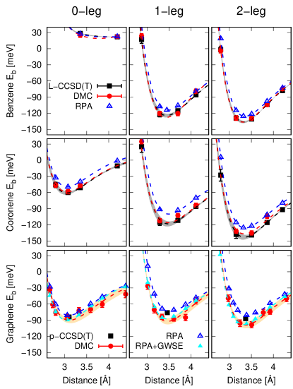
Figure 3: Binding energy curves of water on benzene (top), coronene (middle), and graphene (bottom) in the 0-leg, 1-leg, and 2-leg motifs computed with the many-body electronic structure methods L-CCSD(T), DMC, and RPA. Error bars in DMC correspond to the stochastic error (1 standard deviation), in L-CCSD(T) to the basis set uncertainty (see Appendix B). Dashed lines are fits via a Morse potential (see Appendix C).

Interaction energy curves of water adsorbed in three different configurations (0-leg, 1-leg, 2-leg, see Fig. 2) on benzene, coronene, and graphene have been computed with a range of many-body methods. Here, DMC as well as CCSD(T) are considered benchmark quality methods, while RPA is tested as a cheaper alternative. Due to the smaller unit cell used in p-CCSD(T), we expect that DMC provides the best reference interaction energies for water adsorbed on graphene. Combined interaction energy curves for the considered systems are shown in Fig 3, and interpolated minima are given in Table 2.

We begin by noting that the 0-leg configuration on benzene is purely repulsive (i.e. unbound), while it gets increasingly attractive on coronene and graphene. This behavior will be rationalized in terms of the charge density distribution in section IV. This trend is consistent with all methodologies and DMC and L-CCSD(T) agree within 2 meV for this binding motif. In contrast, both the 1-leg and 2-leg structures bind on benzene, with the 2-leg adsorption 5-11 meV stronger. This binding energy difference increases on coronene to 15-22 meV. This is due to a decreased binding energy of the 1-leg motif (from benzene to coronene), while the 2-leg binding is identical from DMC and RPA and even slightly stronger from L-CCSD(T). In stark contrast to the behavior observed on the small molecules, on periodic graphene the 0-leg, 1-leg, and 2-leg structures have very similar DMC binding energies of $-90\pm 6$, $-92\pm 6$, and $-99\pm 6$ meV, respectively. Interestingly, this includes the 0-leg configuration which on benzene was purely repulsive. The contrast between benzene and graphene for the 0-leg motif is quite remarkable and will be commented on in more detail in section IV.

The benchmark quality methods DMC and L-CCSD(T) agree with each other on the molecular clusters with a maximum error of 12 meV on the single point evaluations and 6 meV for the interpolated binding energies. Similarly, the DMC and CCSD(T) equilibrium binding energies on graphene have only small deviations between 6 and 16 meV. As the two electronic structure methods have quite distinct foundations, this gives us confidence in the high accuracy of the reported binding energies. RPA consistently underbinds all structures by about 9-18 meV, this underestimation is effectively reduced by the singles corrections. The GW based density corrections also change the relative binding of the three motifs, making the 2-leg 8 meV more stable than the 0-leg (in agreement with DMC and CCSD(T)). The observed trend of underestimated RPA binding energies and highly accurate RPA+GWSE energies is consistent with previous findings on molecular adsorption Al-Hamdani et al. (2017a) and molecular crystal lattice energies Klimeš (2016). From the interpolated potential energy curves, we additionally extract the equilibrium adsorption distance and energy (see Table 2). The distances from all many-body methods are in good agreement with each other with a maximum difference of 0.06 Å. Our best DMC estimate for the water adsorption energy on graphene in the lowest energy 2-leg configuration ($-99$ $\pm$6 meV) is in between previously reported binding energies. The p-CCSD(T) adsorption energy is in very good agreement, though the binding is at $-87$ meV slightly lower. This might be due to finite-size or coverage effects (originating from the smaller $4\times 4$ cell employed) and some remaining sensitivity to the basis set. We note that the remaining finite coverage effects have only been corrected for on the level of Hartree-Fock (HF) theory.

Table 2: Equilibrium binding distances $d_{\text{ad}}$ and energies $E_{\text{ad}}$ of single water monomer on benzene, coronene, and graphene from DMC, L-CCSD(T), p-CCSD(T), RPA, and RPA+GWSE. Distances are given in Å and energies in meV.

	DMC			L-CCSD(T)			RPA
	$d_{\text{ad}}$/Å	$E_{\text{ad}}$/meV		$d_{\text{ad}}$/Å	$E_{\text{ad}}$/meV		$d_{\text{ad}}$/Å	$E_{\text{ad}}$/meV
benzene
0-leg	not binding			not binding			not binding
1-leg	3.43(2)	-128(5)		3.45(2)	-124(3)		3.47(1)	-114(3)
2-leg	3.31(1)	-136(5)		3.32(1)	-136(2)		3.35(1)	-126(1)
coronene
0-leg	—	-59(5)		3.05(3)	-61(3)		3.06(1)	-49(2)
1-leg	—	-116(4)		3.48(3)	-118(5)		3.49(1)	-100(4)
2-leg	—	-137(4)		3.34(3)	-143(4)		3.36(1)	-126(2)
	DMC			p-CCSD(T)			RPA			RPA+GWSE
	$d_{\text{ad}}$/Å	$E_{\text{ad}}$/meV		$d_{\text{ad}}$/Å	$E_{\text{ad}}$/meV		$d_{\text{ad}}$/Å	$E_{\text{ad}}$/meV		$d_{\text{ad}}$/Å	$E_{\text{ad}}$/meV
graphene
0-leg	3.10(3)	-90(6)		—	-84		3.09(1)	-81(2)		3.05(1)	-90(2)
1-leg	3.46(3)	-92(6)		—	-76		3.52(1)	-74(1)		3.45(1)	-87(1)
2-leg	3.37(2)	-99(6)		—	-87		3.41(1)	-82(1)		3.33(1)	-98(1)

III.2 Comparison to literature values

As the revised binding energy differs from previously reported values (see Table 1), we carefully investigated the previously used numerical settings and assumptions. First, the difference with the earlier DMC value of $-70\pm 10$ meV Ma et al. (2011), can be explained by the larger statistical errors (smaller precision) and remaining finite-size effects of the older study. On both points, the present study has been improved substantially. Taking this into account, both studies agree within their 95% confidence interval.

The incremental CCSD(T) based adsorption energies are 30 to 35 meV more strongly bound than the DMC values reported here Voloshina et al. (2011). The higher uncertainty of the previous study compared to the DMC and p-CCSD(T) values of this work can be attributed to the basis set employed in the earlier study. Specifically, a mixed double-$\zeta$/triple-$\zeta$ basis set expansion was used and as shown in Appendix B.4 for the water-benzene interaction this does not yield fully converged adsorption energies. Although these basis set tests have been performed with benzene as the substrate and some basis set errors at the HF and correlation level partially cancel, the extent of error cancellation cannot be predicted and we expect a significantly increased accuracy from our p-CCSD(T) calculations.

The other studies listed in Table 1 use finite-sized clusters to approach the periodic system. Given the variation in adsorption energies and different nature of the adsorption bond (see section IV) upon going from benzene, to coronene, to graphene any estimate of the adsorption energy on graphene based on extrapolations from clusters must be done with extreme care.

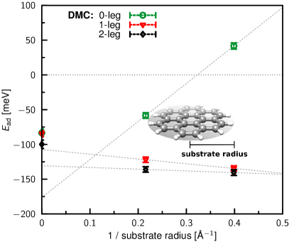
Figure 4: Water adsorption energies at fixed equilibrium distances on graphene, coronene, and benzene plotted as a function of (inverse) substrate size. Following the size definition used in Ref. sub benzene is  0.40 Å^-1 , coronene is 0.22 Å^-1 , and graphene is 0 Å^-1Ḋashed lines are fitted using benzene and coronene data.

Whilst slightly different from earlier studies Rubeš et al. (2009); Jenness et al. (2010), we illustrate the challenge in Fig. 4 where the adsorption energy of the three binding motifs is plotted as a function of cluster size sub . In particular, from Fig. 4 it can be seen that whilst there is a monotonic convergence towards the adsorption energy on graphene for all adsorption motifs, the extrapolation using benzene and coronene data gives a reasonable result only for the 1-leg structure. The extrapolation for both the 0-leg and 2-leg geometries substantially overestimates the adsorption energy and we see a remarkable sensitivity towards the water orientation. Although not reported in the figure this trend is even slightly stronger using the L-CCSD(T) data, where the 2-leg adsorption energy increases from benzene to coronene, i.e. a qualitatively different convergence trend towards graphene dmc . The pronounced contrast in the adsorption energies of the different motifs on small substrates compared to graphene is quite striking. Overall this suggests for such a delicate system as water on graphene adsorption energies obtained directly on periodic models are likely to be more reliable than those obtained with cluster models.

III.3 Implications of revised adsorption energies

Using our reliable benchmark interaction energies, we can now test the capability of standard density functional approximations (DFAs) and a few simplified electronic structure methods for water adsorption on graphene.

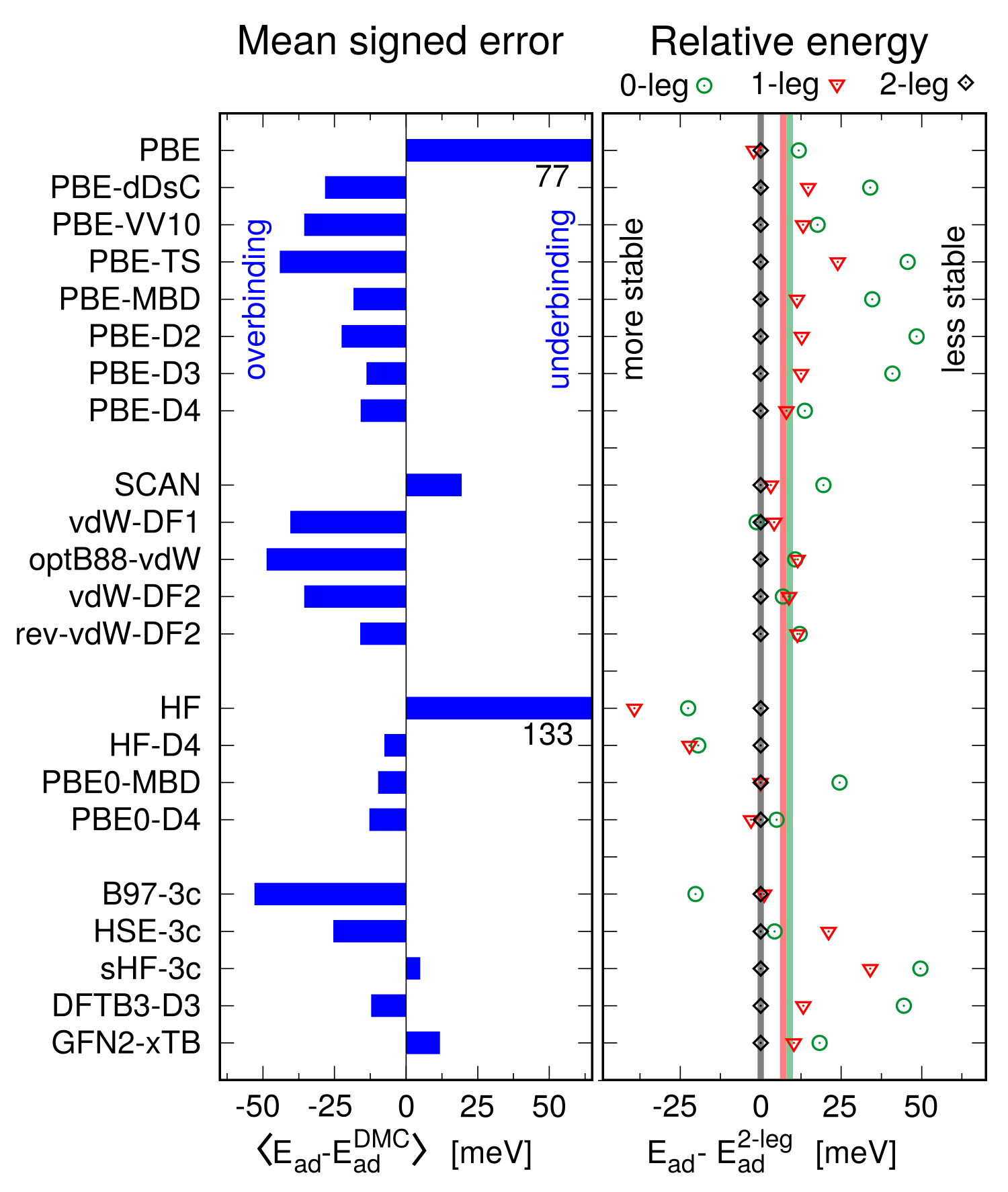
Figure 5: Mean signed errors of water adsorption energies on graphene computed by various DFAs compared to the DMC references are shown (left panel) as well as the relative stability of the three adsorption motifs (right panel, vertical bars correspond to the DMC references). All energies are computed at fixed DMC equilibrium adsorption distances, reported in Table 2. References to individual methods are given in Appendix B.

The performance of the various DFAs is summarized in Fig. 5. We compare to the DMC references and report the mean signed errors (MEs) as well as the relative adsorption energy of the different motifs. While relative energies can sometimes be easier to compute, the different contributions to the intermolecular interactions make this tougher than getting the average interaction correct. The plain PBE functional Perdew et al. (1996) leads to only a rather weak binding for all motifs, clearly long-range vdW interactions are missing. Adding a range of appropriate corrections Klimeš and Michaelides (2012); Grimme et al. (2016); Berland et al. (2015); Hoja et al. (2017) clearly improves the binding. However, the error spread is still significant and the older pairwise schemes (PBE-D2 Grimme (2006), PBE-TS Tkatchenko and Scheffler (2009), PBE-dDsC Steinmann and Corminboeuf (2010), and PBE-VV10 Vydrov and Van Voorhis (2010)) cannot be recommended. Recent developments with vdW corrections pay off and we can see a clear improvement of PBE-MBD Tkatchenko et al. (2012) and PBE-D4 dft over their predecessors. The many-body vdW contributions decrease the binding yielding a better agreement with the DMC references. Most of this effect is already covered at the Axilrod-Teller-Muto type three-body level Axilrod and Teller (1943); Muto (1944) as included in the D3 method Grimme et al. (2010). At the PBE-vdW level, only D4 and VV10 are able to reproduce the relative stability to good accuracy within the DMC stochastic error.

The SCAN functional Sun et al. (2015) is a modern metaGGA that can cover part of the medium-range correlation and has been shown to yield good structures and energies for diversely bonded systems Sun et al. (2016). However, it systematically underbinds all structures, which can partially be compensated by correction schemes Brandenburg et al. (2016a); Peng et al. (2016). Still, due to it’s intrinsic coverage of some vdW forces, it is non-trivial to combine SCAN with correction schemes Hermann and Tkatchenko (2018). Nonlocal vdW functionals of the first generation (vdW-DF1 Dion et al. (2004), optB88-vdW Klimeš et al. (2010)) systematically overbind all binding motifs, as seen before for water inside a carbon nanotube Al-Hamdani et al. (2017b). This is improved in the second generation and vdW-DF2 Lee et al. (2010) and rev-vdW-DF2 Hamada (2014) both give reasonably accurate results. We also note that the relative stabilities of the different binding motifs are much better described using the SCAN functional than for PBE. In order to improve the exchange interactions, fractions of one-determinantal (Fock) exchange are often included in DFAs. Indeed, PBE0 Adamo and Barone (1999) combined with the most successful vdW corrections (D4 and MBD) improve slightly over its GGA pendant. The simplified DFAs (sHF-3c Sure and Grimme (2013); Cutini et al. (2016), HSE-3c Brandenburg et al. (2016b), B97-3c Brandenburg et al. (2018)) give mixed results, overall their accuracy is similar to the average dispersion corrected DFA. As they have been designed for increased computational speed (speedup of up to 2 orders of magnitude) they might still be useful for screening applications Caldeweyher and Brandenburg (2018). The same holds for the tight-binding Hamiltonians (DFTB3-D3 Elstner et al. (1998); Aradi et al. (2007); Gaus et al. (2013); Brandenburg and Grimme (2014), GFN2-xTB Grimme et al. (2017); Bannwarth et al. (2018)), especially GFN2-xTB seems to profit a lot from error compensations. Clearly, many more exchange correlation functionals exist, but benchmarking all variants exceeds the aim of this study.

Large scale dynamics studies of water at graphitic interfaces have been performed in the past years using classical water force fields combined with Lennard-Jones parameters for the oxygen-carbon interaction Hummer et al. (2001); Holt (2006); Kim et al. (2014); McKenzie and Kang (2014); Ma et al. (2015); Radha et al. (2016); Li and Wang (2017). Parameters have been adjusted to reference data from quantum chemistry on graphene-like clusters Wu and Aluru (2013) or by reproducing experimental data like the contact angle of a water droplet on graphite Werder et al. (2003); Leroy et al. (2015). Our study has two major implications apart from an increased scepticism regarding the older theoretical reference data. First, we find that a Morse potential is much better suited to describe the water molecule-graphene interaction compared to Lennard-Jones potentials (Fig. 3 and Appendix A). Furthermore, a coarse-grained model describing the interaction only as a carbon-oxygen interaction cannot describe both the 0-leg and 2-leg adsorption motifs simultaneously, i.e. the hydrogen-carbon interactions are mandatory for a qualitatively correct description. Our new data will be valuable for further potential refinements, though for faithful predictions additional non-equilibrium geometries and high water coverages are needed.

IV Analyzing the nature of the water-graphene interaction

We now briefly discuss the nature of the interaction between water and graphene. As part of our analysis we examined how, at the DFT level, the electronic charge density rearranges upon creation of the adsorption bond. This is shown in Fig. 6 for the three binding motifs.

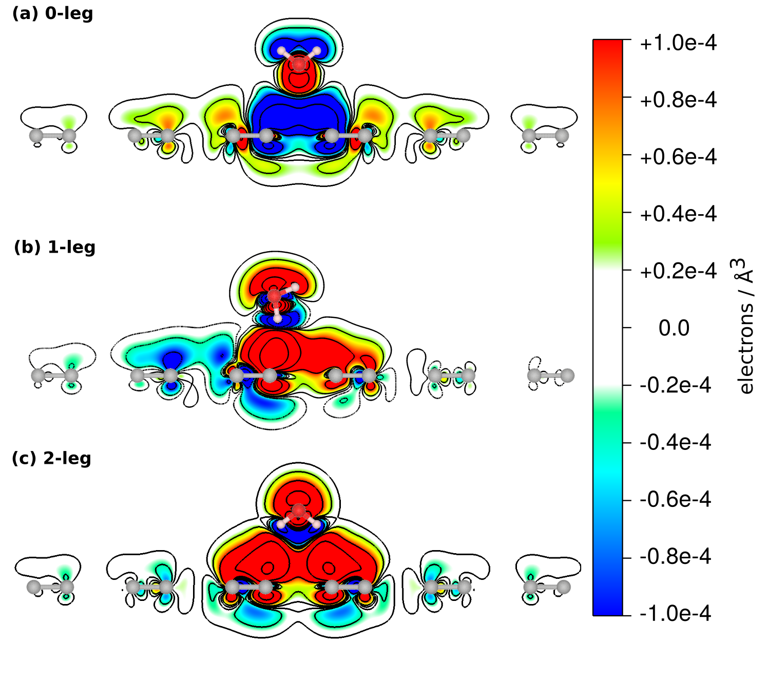
Figure 6: Electronic density change upon binding water on graphene in the equilibrium geometry for the (a) 0-leg, (b) 1-leg, and (c) 2-leg configurations. Planes perpendicular to the surface that bisect the water molecules are shown. Red regions indicate density increase upon binding; blue regions indicate depletion. Electronic density was calculated with DFT, using the PBE functional in a 5$\times$5 unit cell.

Charge density rearrangement plots such as this provide a pictorial representation of how the electron density rearranges upon adsorption. The key features revealed by Fig. 6 are that: (i) The most extensive areas of charge rearrangement are on the water molecule and in the immediate vicinity of each adsorption site; (ii) The extent of the charge density rearrangement is fairly long ranged; carbon atoms as far as 8 Å from the molecule exhibit some (albeit small) change in their charge density; and (iii) In all configurations the electronegative oxygen atom gains charge density, while the hydrogens lose charge density. The key difference between the 0-leg motif and the others is that in the 0-leg structure the negative oxygen ion points towards the graphene layer, and induces a charge loss in the local area surrounding it. Part of the charge is transferred to the water molecule, while the rest is redistributed within the graphene layer. This charge rearrangement in the substrate is slightly more extensive in the 0-leg structure than in the two other binding motifs, which explains in part the strong variation of the 0-leg adsorption energy upon going from benzene to graphene. Note that the qualitatively different nature of the adsorption bond for the 0-leg motif compared to the others has an impact on the surface dipole moment and thus the work function of the subtsrate. Indeed at the water coverage considered, the DFT PBE based work functions are 3.7, 4.5, and 4.8 meV for the 0-leg, 1-leg and 2-leg motifs, respectively. The differences are quite pronounced and could in principle be observable experimentally. In addition, as the molecule rotates on or diffuses across the surface the nature of the charge rearrangement is likely to vary rapidly and so too the work function.

A more quantitative analysis of the adsorption bond has been performed with symmetry adapted perturbation theory for the small substrate models (SAPT Hohenstein and Sherrill (2010); Heßelmann et al. (2005); Jansen (2014); Szalewicz (2012)). The results of this analysis are reported in the Supporting Information. The key conclusion from this analysis is that the electrostatic component to the interaction is attractive for the 1-leg and 2-leg motifs, while it is repulsive for the 0-leg motif on benzene. However, this repulsive interaction decreases significantly for larger substrate sizes and at the same time the attraction from vdW interactions increases. We can overall conclude from this analysis that the 1-leg and 2-leg motifs behave in a rather similar manner, while the 0-leg motif has a quite distinct electrostatic interaction along with a more pronounced charge reorganization in the substrate.

V Conclusions

To conclude, we have computed the adsorption of a water monomer on a periodic graphene sheet with DMC, CCSD(T), and RPA. By comparison to RPA and to L-CCSD(T) on smaller aromatic substrates, we have been able to resolve discrepancies between previously published adsorption energies. We have shown that different water orientations have quite distinct interactions with the graphene layer, but that ultimately they yield very similar binding energies. Cheaper computational methods such as DFT have shown that the potential energy surface for water on graphene is very smooth. However, here we show for the first time from accurate many-body electronic structure methods that there is almost no orientational dependence in the water monomer adsorption energy. Whilst more work is needed, this could have implications for and could partly explain the very low friction coefficient of liquid water on sp²-bonded carbon. Our study also shows that DFAs employing atom-pairwise vdW corrections do a poor job at describing the delicate nature of this adsorption system. However, modern functionals like PBE-D3, PBE-D4, PBE-MBD, and rev-vdW-DF2 perform reasonably well with deviations to the DMC references below chemical accuracy. Even slightly higher accuracy can be achieved with the hybrid functional PBE0-D4. We hope that the benchmark provided here will be of value in larger scale ab initio MD and classical MD studies of water on graphene and other sp²-bonded carbon materials. Together with previous studies using a range of many-body methods to study adsorption on hexagonal boron-nitride (hBN) Al-Hamdani et al. (2017a), carbon nanotubes Al-Hamdani et al. (2017c), clays Zen et al. (2016b), and lithium hydride Binnie et al. (2010); Tsatsoulis et al. (2017), our study demonstrates that adsorption energies on extended surfaces can now be computed with sub-chemical accuracy. These electronic structure approaches are becoming a robust and reliable tool and have the prospect of been applied routinely to surface adsorption problems.

Appendix A Contact angle from molecular dynamics simulations

The simulations to demonstrate the influence of the adsorption energy on the contact angle were done using the coarse-grained mW model Molinero and Moore (2009) of water and a Morse wall potential that acts as a function of the $z$ coordinate. The distance parameter was fitted to reproduce the DMC interaction curve for the 2-leg conformation. The resulting interaction curves, together with Lennard-Jones 9-3 and 12-6 wall variants, can be seen in figure 7a.

To obtain contact angles we performed computations with the LAMMPS Plimpton (1995) software, integrating the equations of motion with a timestep of 10 fs in the $NVT$ ensemble utilizing a 10-fold Nosé-Hoover chain Martyna et al. (1992) with a relaxation time of 1 ps to realize a temperature of 300 K for a total time of 20 ns (an additional initial 10 ns to relax the droplet shape were discarded). From the trajectories we obtained the radial density profile of the liquid and fitted this to a spherical cap shape which yields the contact angle (we did not find any significant deviations from spherical shape). We performed this calculation for droplet sizes ranging from $\sim$ 600 to $\sim$ 70,000 molecules, fitting the size-dependent contact angles to the line-tension modified Young’s equation Boruvka and Neumann (1977):

$$\cos\left(\theta_{R}\right)=\cos\left(\theta_{\mathrm{inf}}\right)-\frac{1}{\gamma_{\mathrm{lv}}}\frac{\tau}{R}$$

which results in the contact angle for an infinitely large water droplet. Here, $\theta_{R}$ is the measured contact angle for a given droplet, $\theta_{\mathrm{inf}}$ is the contact angle of the infinite droplet, $\gamma_{\mathrm{lv}}$ is the liquid vapor surface tension (which does not need to be known for a fit), $\tau$ is the line tension and $R$ is the average radius of the contact area between the droplet and the wall. The results can be seen in Fig. 7b and show a stark influence of the contact angle to the used interaction strength and potential type. The simulation cells were periodic in $x$ and $y$ dimensions and with roughly 40 nm $\times$ 40 nm large enough to avoid self-interaction of the water molecules even for the complete wetting geometry in all cases but for the largest droplets.

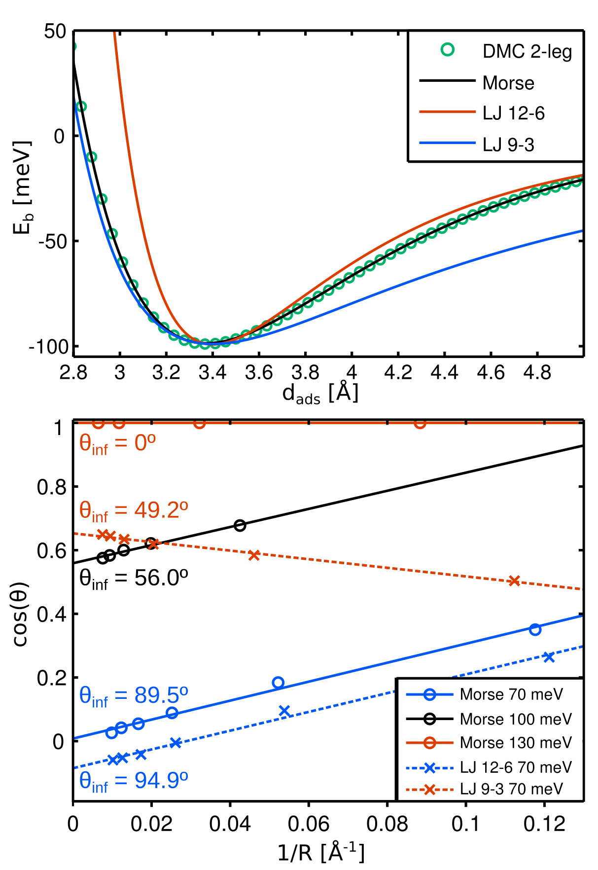
Figure 7: Water adsorption modeled by a coarse-gained water model (mW) and different wall potentials. The upper panel shows the water-wall interaction potentials for an interaction strength of 100 meV. The lower panel shows the results for contact angles of different sized droplets, from which we extract the contact angle $\theta_{\mathrm{inf}}$ for an infinitely large droplet.

Appendix B Computational Details

B.1 System

We consider water adsorption in three different motifs, dubbed 0-leg, 1-leg, and 2-leg as defined in Fig. 2. In order to be consistent with previous DMC calculations, the geometries are taken from PBE Perdew et al. (1996) optimizations, yielding the bond lengths $R(\text{C-C})=1.423$ Å within the graphene sheet, $R(\text{O-H})=0.972$ Å for the hydrogen atom pointing towards the surface in the 1-leg motif and $R(\text{O-H})=0.97$ Å otherwise. The hydrogen atoms of the water molecule have the usual bond angle of $\angle\text{HOH}=104.4^{\circ}$. The adsorption distance $d_{\text{ad}}$ is defined by the distance of oxygen to the graphene plane. Molecular clusters have been cut out of the periodic system and saturated with hydrogens. Here, we use fixed experimental bond lengths of $R(\text{C-C})=1.42$ Å, $R(\text{O-H})=0.957$ Å, and $R(\text{C-H})=1.089$ Å. Based on PBE-D3 calculations, we have tested that the different bond lengths give rise to a binding energy difference below 1.5 meV.

B.2 Density functional theory

DFT calculations have been performed with VASP 5.4.4 Kresse and Furthmüller (1996a, b), Turbomole 7.2 Furche et al. (2014), and Orca 4.0.1 Neese (2012). The numerical integration grids m4 and grid5 for Turbomole and Orca, respectively, have been used. When applicable, the RI-J approximation was used with appropriate auxiliary basis sets Baerends et al. (1973); Dunlap et al. (1979); Eichkorn et al. (1995). Turbomole and Orca employ Gaussian type orbitals and we have computed tightly converged interaction energies for the adsorption on benzene and coronene using PBE in a Dunning type aug-cc-pV5Z basis set expansion Dunning (1989); Kendall et al. (1992). We confirmed that the basis set of def2-QZVPPD quality Weigend et al. (2003); Thakkar et al. (1993) is indeed converged for DFT calculations with deviations from the larger basis set result below 2 meV.

For the periodic system, a 5$\times$5 supercell is constructed with 20 Å vacuum in $z$-direction, energies are evaluated at the $\Gamma$-point, and a dipole correction is used in the $z$-direction. VASP uses projector-augmented plane-waves (PAWs Blöchl (1994); Kresse and Joubert (1999)) with an energy cutoff of 500 eV. Neglecting the dipole correction leads to small deviations of about 2 meV. The convergence of the Brillouin zone sampling has been tested with a 2$\times$2$\times$1 $k$-grid and of the water coverage with a $\Gamma$-point calculation on a 10$\times$10 supercell (both corresponding to 100 points in the Brillouin zone of the primitive graphene cell). The difference between the converged supercell and the 5$\times$5 cell is with 5 meV highest for the 1-leg motif, which we mainly attribute to the remaining dipole interaction in the $x$-$y$-plane that is not present for the other adsorptions due to symmetry. Consistent with RPA and DMC calculations, we use for the water reference the 2-leg geometry and thus accept a bias of up to 5 meV. For the finite sized systems, the dipole correction in the adsorption direction and 20 Å vacuum in all non-periodic directions is used. This setting is compared to the PBE/aug-cc-pV5Z results for the molecular clusters and all interaction energies agree within 2 meV.

For correcting missing long-range van der Waals interactions, we used the D2 Grimme (2006), D3 Grimme et al. (2010), D4 Caldeweyher et al. (2017); dft , VV10 Vydrov and Van Voorhis (2010), dDsC Steinmann and Corminboeuf (2010), TS Tkatchenko and Scheffler (2009), and MBD Tkatchenko et al. (2012) schemes. If not noted otherwise, D3 is used in its rational (Becke-Johnson) damping variant Grimme et al. (2011); Becke and Johnson (2005) and includes the Axilrod-Teller-Muto type three-body term Axilrod and Teller (1943); Muto (1944). As alternative approaches, we use the non-local density based functionals of the vdW-DF1 Dion et al. (2004), vdW-DF2 Lee et al. (2010), rev-vdW-DF2Hamada (2014), and optB86b-vdW Klimeš et al. (2010) types.

B.3 Random phase approximation

We use RPA as implemented in Turbomole 7.2 Furche et al. (2014) for molecular complexes and a developer version of VASP 6 Kresse and Furthmüller (1996a, b) for graphene. The CP corrected complexation energy of $A$ and $B$ in basis sets $a$ and $b$ are computed via

$$E^{\text{int}}_{CP}=E^{\text{int}}+E_{CP}$$ (2)

$$E^{\text{int}}=E(AB_{ab})-E(A_{a})-E(B_{b})$$ (3)

$$E_{CP}=E(A_{a})-E(A_{ab})+E(B_{b})-E(B_{ab})$$ (4)

The Hartree and exact exchange energies (HXX@PBE) and the RPA correlation energy (RPA@PBE) are extrapolated to the basis set limit with optimized exponents Neese et al. (2009). The final interaction energy is given by the extrapolated CP corrected energies $E^{\text{int}}_{CP}$ with a basis set error estimated as $|E_{CP}|/2$. For the periodic system, PAWs with energy cutoff of 430 eV are used. The results were extrapolated to the basis set limit assuming that errors drop off like one over the basis set size Harl and Kresse (2008); Kaltak et al. (2014a). A quadrature with 8 grid points was used for the evaluation of the imaginary time and frequency integrations Kaltak et al. (2014b). The adsorption curves have been computed with 14 Å vacuum corrected with an increased vacuum of 20 Å at the equilibrium geometry. Convergence of the first Brillouin zone sampling has been tested with additional calculations using 2$\times$2$\times$1 $k$-points and a 4$\times$4$\times$1 supercell (the two settings correspond to 25 and 64 points in the Brillouin zone of a primitive graphene cell).

B.4 Coupled cluster theory

We use the linear scaling domain based pair natural orbital CCSD(T) [denoted here as the LCCSD(T)] method Riplinger et al. (2013) as implemented in the ORCA program package Neese (2012). The implementation has been optimized to use compact representations of all amplitudes and imposing block sparsity of tensors Riplinger et al. (2016). Non-augmented basis sets are used in the CCSD(T) calculations to ensure numerically stable convergence on larger substrates. Though convergence of correlation energies with the employed basis sets is well studied Halkier et al. (1998); Truhlar (1998); Jurečka et al. (2006), it is mandatory to carefully test convergence for our target system and numerical settings. In Fig. 8, we show the convergence of uncorrected and CP-corrected Hartree-Fock (HF) and correlation $E_{\text{corr}}$ binding energies.

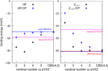
Figure 8: Binding energy separated into HF and correlation ($E^{\text{L-CCSD(T)}}_{\text{corr}}$) contributions for water adsorption on benzene in 2-leg geometry ($d_{\text{ad}}=3.51\,$Å) and increasingly large basis set expansion. Results from a mixed DZ/TZ basis set as in Ref. Voloshina et al. (2011) and extrapolation according to eq. 5 are shown.

As usual for self-consistent field solutions, the plain HF interaction energies overestimate the binding due to basis set superposition error (BSSE). The BSSE is quite effectively removed by the CP correction and for basis sets of about TZ quality can yield reasonably accurate results. Still, the HF calculation is not the bottleneck in our study and we thus use direct extrapolations with QZ and 5Z basis sets Neese et al. (2009) to minimize the associated errors. The basis set artefacts on the correlation energy are more complex. Again, BSSE would lead to an overestimated binding energy, while basis set incompleteness errors typically lead to an underestimated binding energy (missing correlation effects). This can lead to uncorrected correlation energies that are closer to the basis set limit compared to the CP-corrected ones. However, this trend is not clear and the convergence is much smoother using the CP-corrected energies (see Fig. 8), which makes the extrapolation more reliable. In our study, the CCSD(T) correlation energies are extrapolated using the largest basis set results from L-CCSD(T) and extrapolating it with RPA correlation energies in the multiplicative scheme

$$\footnotesize E_{\text{corr}}[\text{CC/CSB}]=E_{\text{corr}}(\text{CC/QZ})\times\frac{E_{\text{corr}}(\text{RPA/CBS})}{E_{\text{corr}}(\text{RPA/QZ})}\normalsize$$ (5)

The CP corrected energies are reported as final results; the non-CP corrected ones give an indication of the basis set completeness. The extrapolation scheme has been chosen to minimize this error estimate (compared to e.g. the additive scheme). For benzene adsorption, we compared this to direct cc-pV(QZ,5Z) extrapolations and deviations in binding energies are below 1 meV (see Fig. 8). In contrast, a previously used combination of DZ and TZ basis sets (setting identical to Ref. Voloshina et al. (2011)) have errors of about 30 meV for the correlation energy. This partially cancels with errors on the HF energy, however, due to the functionally different convergence of HF and $E_{\text{corr}}$ we shouldn’t expect this cancellation to be consistent for different system sizes. Errors in our L-CCSD(T) energies due to pair-thresholds and non-canonical triples (T0) are estimated for benzene adsorption by comparison to conventional CCSD(T) in cc-pVTZ basis to be below 5 meV, which is comparable to previous tests Al-Hamdani et al. (2017a); Guo et al. (2018). Overall, the errors introduced by the truncation, the non-canonical triples, and the basis set extrapolation seem to be under control and below 10 meV.

Periodic CCSD(T) calculations have been carried out following the strategy outlined in Ref. Gruber et al. (2018) employing a slightly smaller 4$\times$4 graphene cell. Periodic HF orbitals have been computed in a PAW basis with an kinetic energy cutoff for the plane wave basis of 500 eV, whereas virtual orbitals in the CCSD calculations are projected to a pseudized aug-cc-pVTZ basis set, in a PAW representation Booth et al. (2016). Perturbative triples (T) are evaluated using the smaller cc-pVDZ basis set to represent the virtual orbitals. The CP corrected interaction energy is defined as

$$E_{\text{int}}=E_{\text{H${}_{2}$O+Graphene}}-E_{\text{H${}_{2}$O}}-E_{\text{Graphene}}.$$ (6)

Finite-size corrections have been computed at the CCSD level Liao and Grüneis (2016) (-17, -16 and -19 meV for the 0-,1- and 2-leg structure, respectively). Finite coverage effects are corrected for at the HF level only using a $5\times 5$ graphene cell (-2, 1 and 2 meV for the 0-,1- and 2-leg structure, respectively). Corrections to the vacuum size are computed using a supercell with a 30 Å vacuum distance at the MP2 level (6, 8 and 7 meV for the 0-,1- and 2-leg structure, respectively). A basis set correction is also included and is defined as the difference between the full plane-wave basis set calculation and the aug-cc-pVTZ one at the MP2 level (-4, -5 and -5 meV for the 0-,1- and 2-leg structure, respectively).

B.5 Quantum Monte Carlo

DMC calculations were performed with the CASINO code Needs et al. (2010). The adsorption energy $E_{\text{ad}}$ is calculated as prescribed in Eq. 1, with $d_{\text{far}}\sim 10$ Å. This evaluation is more efficient than the use of the separate fragments in place of the far away configuration, as it reduces the time step bias Zen et al. (2016a). However, the system at $d_{\text{far}}\sim 10$ Å could have a little residual interaction energy, which was evaluated via L-CCSD(T) to be 2.2 meV for the water-benzene system and 5.5 meV for the water-coronene system. Thus, the DMC evaluations were corrected for this interaction energy, in order to facilitate the comparison with the binding energies obtained via L-CCSD(T) and RPA, which took as reference the energy of the isolated fragments. For the graphene adsorption this residual interaction diminishes well below 1 meV as estimated by DFT calculations (PBE-D3 and PBE-MBD). Similar to Refs. Ma et al. (2009, 2011), we used Dirac-Fock pseudopotentials Trail and Needs (2005a, b) with the locality approximation Mitas et al. (1991). Single particle wave functions were obtained using DFT with the LDA functional and a plane-wave cutoff of 600 Ry, re-expanded in terms of B-splines Alfè and Gillan (2004) with the natural grid spacing $a=\pi/G_{\rm max}$, where $G_{\rm max}$ is the magnitude of the largest plane wave in the expansion. The Jastrow factor used in the trial wavefunction of the system included a two-body electron-electron (e-e) term; two-body electron-nucleus (e-n) terms and three-body electron-electron-nucleus (e-e-n) terms specific for any atom type. The variational parameters of the Jastrow have been optimized in order to minimize the variational variance. The time step dependence has been investigated explicitly considering values of $\tau$ ranging from $10^{-1}$ au to $10^{-3}$ au for a subset of configurations, as reported in the Supporting Information. Production calculations for water-benzene and water-coronene systems used a time step of 0.01 au, and in water-graphene we used $\tau=0.025$ au. These values give a bias smaller than the stochastic error. DMC calculations were performed with a population of tens of thousands of walkers or more. We tested the population bias, which appears to be negligible with respect to the stochastic error in the production calculations (the population bias becomes of the order of a few meV only for a population of a few hundred walkers) as shown in the Supporting Information. In this work we are evaluating the interaction energy as the difference of two configurations both affected by FSE, thus we will benefit from a large FSE cancellation, as observed in other systems Zen et al. (2016b); Al-Hamdani et al. (2017a). Similar to Ref. Zen et al., 2016b, we have estimated the residual FSE correction using the approach of Kwee, Zhang and Krakauer Kwee et al. (2008) (KZK). In a subset of the configurations we checked the reliability of KZK against the more accurate (and computationally more expensive) model periodic Coulomb (MPC) approach Fraser et al. (1996); Williamson et al. (1997); Kent et al. (1999). The estimated FSE correction on DMC binding values are reported in fig. 9.

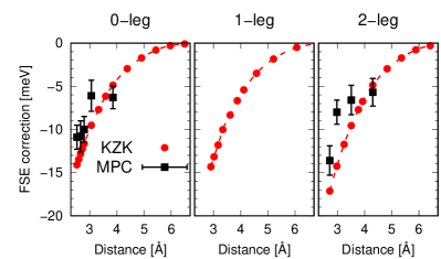
Figure 9: FSE correction in DMC for the interaction energy of water on graphene, as obtained using KZK Kwee et al. (2008) and MPC Fraser et al. (1996); Williamson et al. (1997); Kent et al. (1999) approaches, shown as a function of the distance between the oxygen of water and the graphene sheet.

Appendix C Fit with Morse potential

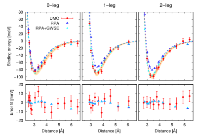
Figure 10: Adsorption energy (top) of water on graphene and difference (bottom) with respect to the fitted Morse potential (dashed lines).

Figure 11: Adsorption energy (top) of water on benzene and difference (bottom) with respect to the fitted Morse potential (dashed lines). A cubic spline is used for the non-binding 0-leg motif.

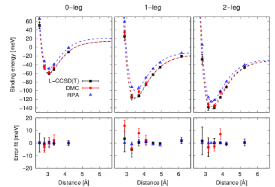
Figure 12: Adsorption energy (top) of water on coronene and difference (bottom) with respect to the fitted Morse potential (dashed lines).

The dissociation curve of water on graphene was fitted using a Morse potential

$$\footnotesize E_{\text{b}}(d)=D_{e}\left[\left(1-e^{-a(d-d_{\text{min}})}\right)^{2}-1\right]+D_{\text{o}}\,,\normalsize$$ (7)

where $d$ is the distance of the water oxygen from graphene (see Fig 2), and the parameters $D_{e}$, $a$, $d_{\text{min}}$ and $D_{o}$ are fitted independently for each of the three motifs. Lower panels of Fig. 10 show that in the range of distances considered in this work the agreement is optimal for $D_{\text{o}}=0$, as the RPA and RPA+GSWE values are within 2 meV from the fit for $d$ close to $d_{\text{min}}$. The values of $E_{\text{ad}}$ and $d_{\text{min}}$ reported in Table 2, and the associated errors, are obtained from the fit, and in particular from the parameters $-D_{e}+D_{o}$ and $d_{\text{min}}$. A Morse potential is used also for the binding curve of benzene, see Fig. 11, and coronene, see Fig. 12. However, in these two cases the Morse potential needs an offset $D_{o}$, as the binding curve converge to zero with a long tail. The lower panels in Figs. 11 and 12 show optimal agreement between the computed values and the Morse potential in the considered range of distances. The values of $E_{\text{ad}}$ reported in Table 2 is calculated as $E_{\text{ad}}=-D_{e}+D_{\text{o}}$, and the associated error is the square root of the sum of squares of the fitting errors. This is a conservative estimation of the error, as $D_{e}$ and $D_{\text{o}}$ are anti-correlated. All Morse parameters are reported in the supporting information, which we recommend for benchmarking approximate methods.

References

- Fumagalli et al. (2018) L. Fumagalli, A. Esfandiar, R. Fabregas, S. Hu, P. Ares, A. Janardanan, Q. Yang, B. Radha, T. Taniguchi, K. Watanabe, G. Gomila, K. S. Novoselov, and A. K. Geim, Science (New York, NY) 360, 1339 (2018).
- Abraham et al. (2017) J. Abraham, K. S. Vasu, C. D. Williams, K. Gopinadhan, Y. Su, C. T. Cherian, J. Dix, E. Prestat, S. J. Haigh, I. V. Grigorieva, P. Carbone, A. K. Geim, and R. R. Nair, Nature Nanotechnology 12, 546 (2017).
- Joshi et al. (2014) R. K. Joshi, P. Carbone, F. C. Wang, V. G. Kravets, Y. Su, I. V. Grigorieva, H. A. Wu, A. K. Geim, and R. R. Nair, Science 343, 752 (2014).
- Nair et al. (2012) R. R. Nair, H. A. Wu, P. N. Jayaram, I. V. Grigorieva, and A. K. Geim, Science 335, 442 (2012).
- Algara-Siller et al. (2015) G. Algara-Siller, O. Lehtinen, F. C. Wang, R. R. Nair, U. Kaiser, H. A. Wu, A. K. Geim, and I. V. Grigorieva, Nature 519, 443 (2015).
- Secchi et al. (2016) E. Secchi, S. Marbach, A. Niguès, D. Stein, A. Siria, and L. Bocquet, Nature 537, 210 (2016).
- Radha et al. (2016) B. Radha, A. Esfandiar, F. C. Wang, A. P. Rooney, K. Gopinadhan, A. Keerthi, A. Mishchenko, A. Janardanan, P. Blake, L. Fumagalli, M. Lozada-Hidalgo, S. Garaj, S. J. Haigh, I. V. Grigorieva, H. A. Wu, and A. K. Geim, Nature 538, 222 (2016).
- Siria et al. (2017) A. Siria, M.-L. Bocquet, and L. Bocquet, Nature Reviews Chemistry 1, 0091 (2017).
- Yoshida et al. (2018) H. Yoshida, V. Kaiser, B. Rotenberg, and L. Bocquet, Nature Communications 9, 1496 (2018).
- Hummer et al. (2001) G. Hummer, J. C. Rasaiah, and J. P. Noworyta, Nature 414, 188 (2001).
- Strogatz et al. (2005) S. H. Strogatz, D. M. Abrams, A. McRobie, B. Eckhardt, and E. Ott, Nature 438, 43 (2005).
- Holt (2006) J. K. Holt, Science (New York, NY) 312, 1034 (2006).
- Tocci et al. (2014) G. Tocci, L. Joly, and A. Michaelides, Nano Lett. 14, 6872 (2014).
- Michaelides (2016) A. Michaelides, Nature 537, 171 (2016).
- Esfandiar et al. (2017) A. Esfandiar, B. Radha, F. C. Wang, Q. Yang, S. Hu, S. Garaj, R. R. Nair, A. K. Geim, and K. Gopinadhan, Science (New York, NY) 358, 511 (2017).
- Björneholm et al. (2016) O. Björneholm, M. H. Hansen, A. Hodgson, L.-M. Liu, D. T. Limmer, A. Michaelides, P. Pedevilla, J. Rossmeisl, H. Shen, G. Tocci, E. Tyrode, M.-M. Walz, J. Werner, and H. Bluhm, Chem. Rev. 116, 7698 (2016).
- Ma et al. (2011) J. Ma, A. Michaelides, D. Alfè, L. Schimka, G. Kresse, and E. Wang, Phys. Rev. B 84, 033402 (2011).
- Hamada (2012) I. Hamada, Phys. Rev. B 86, 195436 (2012).
- Silvestrelli and Ambrosetti (2014) P. L. Silvestrelli and A. Ambrosetti, J. Chem. Phys. 140, 124107 (2014).
- (20) M. Lorenz, B. Civalleri, L. Maschio, M. Sgroi, and D. Pullini, J. Comput. Chem. 35, 1789.
- Rubeš et al. (2009) M. Rubeš, P. Nachtigall, J. Vondrášek, and O. Bludský, J. Phys. Chem. C 113, 8412 (2009).
- Jenness et al. (2010) G. R. Jenness, O. Karalti, and K. D. Jordan, Phys. Chem. Chem. Phys. 12, 6375 (2010).
- Voloshina et al. (2011) E. Voloshina, D. Usvyat, M. Schutz, Y. Dedkov, and B. Paulus, Phys. Chem. Chem. Phys. 13, 12041 (2011).
- Michaelides et al. (2015) A. Michaelides, T. J. Martinez, A. Alavi, G. Kresse, and F. R. Manby, J. Chem. Phys. 143, 102601 (2015).
- Feller and Jordan (2000) D. Feller and K. D. Jordan, J. Phys. Chem. A 104, 9971 (2000).
- Note (1) Ideally, the energy for non-interacting systems should be evaluated at a distance . Computationally, there are two alternative ways to calculate : i. consider a finite value of that makes the residual interaction energy negligible with respect to the needed accuracy; ii. evaluate as the summation of the energy of the water and graphene fragments. The two methods are in principle equivalent for size-consistent electronic structure approaches, however in periodic systems (so, in presence of finite size errors) the former method typically benefits from a better error cancellation and allows the use of smaller simulation cells. Details are discussed in Appendix B.
- Foulkes et al. (2001) W. M. C. Foulkes, L. Mitas, R. J. Needs, and G. Rajagopal, Rev. Mod. Phys. 73, 33 (2001).
- Zen et al. (2016a) A. Zen, S. Sorella, M. J. Gillan, A. Michaelides, and D. Alfè, Phys. Rev. B 93, 241118(R) (2016a).
- Zen et al. (2018) A. Zen, J. G. Brandenburg, J. Klimeš, A. Tkatchenko, D. Alfè, and A. Michaelides, Proc. Natl. Acad. Sci. U.S.A. 115, 1724 (2018).
- Needs et al. (2010) R. J. Needs, M. D. Towler, N. D. Drummond, and P. L. Rios, J. Phys.: Condens. Matter 22, 023201 (2010).
- Riplinger et al. (2013) C. Riplinger, B. Sandhoefer, A. Hansen, and F. Neese, J. Chem. Phys. 139, 134101 (2013).
- Neese (2012) F. Neese, WIREs Comput. Mol. Sci. 2, 73 (2012).
- Booth et al. (2013) G. H. Booth, A. Grüneis, G. Kresse, and A. Alavi, Nature 493, 365 (2013).
- Kresse and Furthmüller (1996a) G. Kresse and J. Furthmüller, J. Comp. Mat. Sci. 6, 15 (1996a).
- Kresse and Furthmüller (1996b) G. Kresse and J. Furthmüller, Phys. Rev. B 54, 11169 (1996b).
- Hummel et al. (2017) F. Hummel, T. Tsatsoulis, and A. Grüneis, J. Chem. Phys. 146, 124105 (2017).
- Gruber et al. (2018) T. Gruber, K. Liao, T. Tsatsoulis, F. Hummel, and A. Grüneis, Phys. Rev. X 8, 021043 (2018).
- Nozières and Pines (1958) P. Nozières and D. Pines, Phys. Rev. 111, 442 (1958).
- Harl and Kresse (2008) J. Harl and G. Kresse, Phys. Rev. B 77, 045136 (2008).
- Harl and Kresse (2009) J. Harl and G. Kresse, Phys. Rev. Lett. 103, 056401 (2009).
- Eshuis et al. (2012) H. Eshuis, J. E. Bates, and F. Furche, Theo. Chem. Acc. 131, 1084 (2012).
- Wilhelm et al. (2016) J. Wilhelm, P. Seewald, M. Del Ben, and J. Hutter, J. Chem. Theory Comput. 12, 5851 (2016).
- Schimka et al. (2010) L. Schimka, J. Harl, A. Stroppa, A. Grüneis, M. Marsman, F. Mittendorfer, and G. Kresse, Nat. Mater. 9, 741 (2010).
- Ren et al. (2011) X. Ren, A. Tkatchenko, P. Rinke, and M. Scheffler, Phys. Rev. Lett. 106, 153003 (2011).
- Klimeš (2016) J. Klimeš, J. Chem. Phys. 145, 094506 (2016).
- Klimeš et al. (2015) J. Klimeš, M. Kaltak, E. Maggio, and G. Kresse, J. Chem. Phys. 143, 102816 (2015).
- Al-Hamdani et al. (2017a) Y. S. Al-Hamdani, M. Rossi, D. Alfè, T. Tsatsoulis, B. Ramberger, J. G. Brandenburg, A. Zen, G. Kresse, A. Grüneis, A. Tkatchenko, and A. Michaelides, J. Chem. Phys. 147, 044710 (2017a).
- (48) We define the substrate size as the circle in the substrate plane with minimal radius, where all atom positions are within the circle (see inset of Fig. 4).
- (49) Note that this trend is still possible within the stochastic error of the DMC data.
- Perdew et al. (1996) J. P. Perdew, K. Burke, and M. Ernzerhof, Phys. Rev. Lett. 77, 3865 (1996), erratum Phys. Rev. Lett. 78, 1396 (1997).
- Klimeš and Michaelides (2012) J. Klimeš and A. Michaelides, J. Chem. Phys. 137, 120901 (2012).
- Grimme et al. (2016) S. Grimme, A. Hansen, J. G. Brandenburg, and C. Bannwarth, Chem. Rev. 116, 5105 (2016).
- Berland et al. (2015) K. Berland, V. R. Cooper, K. Lee, E. Schröder, T. Thonhauser, P. Hyldgaard, and B. I. Lundqvist, Rep. Prog. Phys. 78, 066501 (2015).
- Hoja et al. (2017) J. Hoja, A. M. Reilly, and A. Tkatchenko, WIREs Comput. Mol. Sci. 7, e1294 (2017).
- Grimme (2006) S. Grimme, J. Comput. Chem. 27, 1787 (2006).
- Tkatchenko and Scheffler (2009) A. Tkatchenko and M. Scheffler, Phys. Rev. Lett. 102, 073005 (2009).
- Steinmann and Corminboeuf (2010) S. N. Steinmann and C. A. Corminboeuf, J. Chem. Theory Comput. 6, 1990 (2010).
- Vydrov and Van Voorhis (2010) O. A. Vydrov and T. Van Voorhis, J. Chem. Phys. 133, 244103 (2010).
- Tkatchenko et al. (2012) A. Tkatchenko, R. A. DiStasio., R. Car, and M. Scheffler, Phys. Rev. Lett. 108, 236402 (2012).
- (60) DFT-D4 model will be published elsewhere. It is based on Ref. Caldeweyher et al. (2017) and includes all dipole many-body orders.
- Axilrod and Teller (1943) B. M. Axilrod and E. Teller, J. Chem. Phys. 11, 299 (1943).
- Muto (1944) Y. Muto, Proc. Phys. Math. Soc. Jpn. 17, 629 (1944).
- Grimme et al. (2010) S. Grimme, J. Antony, S. Ehrlich, and H. Krieg, J. Chem. Phys. 132, 154104 (2010).
- Sun et al. (2015) J. Sun, A. Ruzsinszky, and J. P. Perdew, Phys. Rev. Lett. 115, 036402 (2015).
- Sun et al. (2016) J. Sun, R. Remsing, Y. Zhang, Z. Sun, A. Ruzsinszky, H. Peng, Z. Yang, A. Paul, U. Waghmare, X. Wu, M. L. Klein, and J. P. Perdew, Nat. Chem. 8, 831 (2016).
- Brandenburg et al. (2016a) J. G. Brandenburg, J. E. Bates, J. Sun, and J. P. Perdew, Phys. Rev. B 94, 115144 (2016a).
- Peng et al. (2016) H. Peng, Z.-H. Yang, J. P. Perdew, and J. Sun, Phys. Rev. X 6, 041005 (2016).
- Hermann and Tkatchenko (2018) J. Hermann and A. Tkatchenko, J. Chem. Theory Comput. 14, 1361 (2018).
- Dion et al. (2004) M. Dion, H. Rydberg, E. Schröder, D. C. Langreth, and B. I. Lundqvist, Phys. Rev. Lett. 92, 246401 (2004).
- Klimeš et al. (2010) J. Klimeš, D. R. Bowler, and A. Michaelides, J. Phys.: Condens. Matter 22, 022201 (2010).
- Al-Hamdani et al. (2017b) Y. S. Al-Hamdani, D. Alfè, and A. Michaelides, J. Chem. Phys. 146, 094701 (2017b).
- Lee et al. (2010) K. Lee, E. D. Murray, L. Kong, B. I. Lundqvist, and D. C. Langreth, Phys. Rev. B 82, 081101 (2010).
- Hamada (2014) I. Hamada, Phys. Rev. B 89, 121103(R) (2014).
- Adamo and Barone (1999) C. Adamo and V. Barone, J. Chem. Phys. 110, 6158 (1999).
- Sure and Grimme (2013) R. Sure and S. Grimme, J. Comput. Chem. 34, 1672 (2013).
- Cutini et al. (2016) M. Cutini, B. Civalleri, M. Corno, R. Orlando, J. G. Brandenburg, L. Maschio, and P. Ugliengoa, J. Chem. Theory Comput. 12, 3340 (2016).
- Brandenburg et al. (2016b) J. G. Brandenburg, E. Caldeweyher, and S. Grimme, Phys. Chem. Chem. Phys. 18, 15519 (2016b).
- Brandenburg et al. (2018) J. G. Brandenburg, C. Bannwarth, A. Hansen, and S. Grimme, J. Chem. Phys. 148, 064104 (2018).
- Caldeweyher and Brandenburg (2018) E. Caldeweyher and J. G. Brandenburg, J. Phys.: Condens. Matter 30, 213001 (2018).
- Elstner et al. (1998) M. Elstner, D. Porezag, G. Jungnickel, J. Elsner, M. Haugk, T. Frauenheim, S. Suhai, and G. Seifert, Phys. Rev. B 58, 7260 (1998).
- Aradi et al. (2007) B. Aradi, B. Hourahine, and T. Frauenheim, J. Phys. Chem. A 111, 5678 (2007).
- Gaus et al. (2013) M. Gaus, A. Goez, and M. Elstner, J. Chem. Theory Comput. 9, 338 (2013).
- Brandenburg and Grimme (2014) J. G. Brandenburg and S. Grimme, J. Phys. Chem. Lett. 5, 1785 (2014).
- Grimme et al. (2017) S. Grimme, C. Bannwarth, and P. Shushkov, J. Chem. Theory Comput. 13, 1989 (2017).
- Bannwarth et al. (2018) C. Bannwarth, S. Ehlert, and S. Grimme, (2018), 10.26434/chemrxiv.7246238.v1.
- Kim et al. (2014) H.-Y. Kim, M. C. dos Santos, and M. W. Cole, J. Phys. Chem. A 118, 8237 (2014).
- McKenzie and Kang (2014) S. McKenzie and H. C. Kang, Phys. Chem. Chem. Phys. 16, 26004 (2014).
- Ma et al. (2015) M. Ma, G. Tocci, A. Michaelides, and G. Aeppli, Nature Materials 15, 66 (2015).
- Li and Wang (2017) J. Li and F. Wang, J. Chem. Phys. 146, 054702 (2017).
- Wu and Aluru (2013) Y. Wu and N. R. Aluru, J. Phys. Chem. B 117, 8802 (2013).
- Werder et al. (2003) T. Werder, J. H. Walther, R. L. Jaffe, T. Halicioglu, and P. Koumoutsakos, J. Phys. Chem. B 107, 1345 (2003).
- Leroy et al. (2015) F. Leroy, S. Liu, and J. Zhang, J. Phys. Chem. C 119, 28470 (2015).
- Hohenstein and Sherrill (2010) E. G. Hohenstein and C. D. Sherrill, J. Chem. Phys. 132, 184111 (2010).
- Heßelmann et al. (2005) A. Heßelmann, G. Jansen, and M. Schütz, J. Chem. Phys. 122, 014103 (2005).
- Jansen (2014) G. Jansen, WIREs Comput. Mol. Sci. 4, 127 (2014).
- Szalewicz (2012) K. Szalewicz, WIREs Comput. Mol. Sci. 2, 254 (2012).
- Al-Hamdani et al. (2017c) Y. S. Al-Hamdani, D. Alfè, and A. Michaelides, J. Chem. Phys. 146, 094701 (2017c).
- Zen et al. (2016b) A. Zen, L. M. Roch, S. J. Cox, X. L. Hu, S. Sorella, D. Alfè, and A. Michaelides, J. Phys. Chem. C 120, 26402 (2016b).
- Binnie et al. (2010) S. J. Binnie, S. J. Nolan, N. D. Drummond, D. Alfè, N. L. Allan, F. R. Manby, and M. J. Gillan, Phys. Rev. B 82, 165431 (2010).
- Tsatsoulis et al. (2017) T. Tsatsoulis, F. Hummel, D. Usvyat, M. Schütz, G. H. Booth, S. S. Binnie, M. J. Gillan, D. Alfè, A. Michaelides, and A. Grüneis, J. Chem. Phys. 146, 204108 (2017).
- Molinero and Moore (2009) V. Molinero and E. B. Moore, J. Phys. Chem. B 113, 4008 (2009).
- Plimpton (1995) S. Plimpton, J. Comput. Phys. 117, 1 (1995).
- Martyna et al. (1992) G. J. Martyna, M. L. Klein, and M. Tuckerman, J. Chem. Phys. 97, 2635 (1992).
- Boruvka and Neumann (1977) L. Boruvka and A. Neumann, J. Chem. Phys. 66, 5464 (1977).
- Furche et al. (2014) F. Furche, R. Ahlrichs, C. Hättig, W. Klopper, M. Sierka, and F. Weigend, WIREs Comput Mol Sci 4, 91 (2014).
- Baerends et al. (1973) E. J. Baerends, D. E. Ellis, and P. Ros, Chem. Phys. 2, 41 (1973).
- Dunlap et al. (1979) B. I. Dunlap, W. D. Connolly, and J. R. Sabin, J. Chem. Phys. 71, 3396 (1979).
- Eichkorn et al. (1995) K. Eichkorn, O. Treutler, H. Öhm, M. Häser, and R. Ahlrichs, Chem. Phys. Lett. 240, 283 (1995).
- Dunning (1989) T. H. Dunning, Jr., J. Chem. Phys. 90, 1007 (1989).
- Kendall et al. (1992) R. A. Kendall, T. H. Dunning, Jr., and R. J. Harrison, J. Chem. Phys. 96, 6796 (1992).
- Weigend et al. (2003) F. Weigend, F. Furche, and R. Ahlrichs, J. Chem. Phys. 119, 12753 (2003).
- Thakkar et al. (1993) A. J. Thakkar, T. Koga, M. Saito, and R. E. Hoffmeyer, Int. J. Quantum Chem. Symp. 48, 343 (1993).
- Blöchl (1994) P. E. Blöchl, Phys. Rev. B 50, 17953 (1994).
- Kresse and Joubert (1999) G. Kresse and J. Joubert, Phys. Rev. B 59, 1758 (1999).
- Caldeweyher et al. (2017) E. Caldeweyher, C. Bannwarth, and S. Grimme, J. Chem. Phys. 147, 034112 (2017).
- Grimme et al. (2011) S. Grimme, S. Ehrlich, and L. Goerigk, J. Comput. Chem. 32, 1456 (2011).
- Becke and Johnson (2005) A. D. Becke and E. R. Johnson, J. Chem. Phys. 123, 154101 (2005).
- Neese et al. (2009) F. Neese, A. Hansen, and D. G. Liakos, J. Chem. Phys. 131, 064103 (2009).
- Kaltak et al. (2014a) M. Kaltak, J. Klimeš, and G. Kresse, J. Chem. Theo. Comput. 10, 2498 (2014a).
- Kaltak et al. (2014b) M. Kaltak, J. Klimeš, and G. Kresse, Phys. Rev. B 90, 054115 (2014b).
- Riplinger et al. (2016) C. Riplinger, P. Pinski, U. Becker, E. F. Valeev, and F. Neese, J. Chem. Phys. 144, 024109 (2016).
- Halkier et al. (1998) A. Halkier, T. Helgaker, P. Jørgensen, W. Klopper, H. Koch, J. Olsen, and A. K. Wilson, Chem. Phys. Lett. 286, 243 (1998).
- Truhlar (1998) D. G. Truhlar, Chem. Phys. Lett. 294, 45 (1998).
- Jurečka et al. (2006) P. Jurečka, J. Šponer, J. Cerny, and P. Hobza, Phys. Chem. Chem. Phys. 8, 1985 (2006).
- Guo et al. (2018) Y. Guo, C. Riplinger, U. Becker, D. G. Liakos, Y. Minenkov, L. Cavallo, and F. Neese, J. Chem. Phys. 148, 011101 (2018).
- Booth et al. (2016) G. H. Booth, T. Tsatsoulis, G. K.-L. Chan, and A. Grüneis, The Journal of Chemical Physics 145, 084111 (2016).
- Liao and Grüneis (2016) K. Liao and A. Grüneis, J. Chem. Phys. 145, 141102 (2016).
- Ma et al. (2009) J. Ma, D. Alfè, A. Michaelides, and E. Wang, J. Chem. Phys. 130, 154303 (2009).
- Trail and Needs (2005a) J. R. Trail and R. J. Needs, J. Chem. Phys. 122, 014112 (2005a).
- Trail and Needs (2005b) J. R. Trail and R. J. Needs, J. Chem. Phys. 122, 174109 (2005b).
- Mitas et al. (1991) L. Mitas, E. L. Shirley, and D. M. Ceperley, J. Chem. Phys. 95, 3467 (1991).
- Alfè and Gillan (2004) D. Alfè and M. J. Gillan, Phys. Rev. B 70, 161101 (2004).
- Kwee et al. (2008) H. Kwee, S. Zhang, and H. Krakauer, Phys. Rev. Lett. 100, 126404 (2008).
- Fraser et al. (1996) L. M. Fraser, W. M. C. Foulkes, G. Rajagopal, R. J. Needs, S. D. Kenny, and A. J. Williamson, Phys. Rev. B 53, 1814 (1996).
- Williamson et al. (1997) A. J. Williamson, G. Rajagopal, R. J. Needs, L. M. Fraser, W. M. C. Foulkes, Y. Wang, and M.-Y. Chou, Phys. Rev. B 55, R4851 (1997).
- Kent et al. (1999) P. R. C. Kent, R. Q. Hood, A. J. Williamson, R. J. Needs, W. M. C. Foulkes, and G. Rajagopal, Phys. Rev. B 59, 1917 (1999).