Correction to the energy spectrum of ${}^{1}S_{0}$ heavy quarkonia due to two-gluon annihilation effect

Abstract

In this work, the non-relativistic asymptotic behavior of the transition $q\overline{q}\rightarrow 2g\rightarrow q\overline{q}$ in the ${}^{1}S_{0}$ channel is discussed. Different with the usual calculation which expands the physical amplitude around the quark anti-quark threshold, we take the quark anti-quark pairs as off shell and only expand the expression on the three-dimensional momenta of the quarks and anti-quarks. We calculate the results to order 6. The imagine part of the results after applying the on shell conditions can reproduce the non-relativistic QCD (NRQCD) results in leading order of $\alpha_{s}$. The real part of the results can be used to estimate the mass shift of the ${}^{1}S_{0}$ heavy quark anti-quark system due to the $2g$ annihilation effect. The results can also be used to estimate the energy shifts of the positronium system due to the two-photon annihilation.

I Introduction

The energy spectrum of quarkonia is a basic topic of the strong interaction. Many phenomenological methods have been applied to study this topic for a long time such as quark modelquark-model , QCD sum rulesQCD-sumrule , Dyson-Schwinger equation and Bethe-Salpeter equation BS-eq and unitary chiral modelchiral-unitary etc.. Due to the asymptotic freedom of the QCD and the large masses of the heavy quarks ($c$ quark and $b$ quark), the heavy quarkonia provides a special window to study the QCD since both the pertuabtive behavior and the non-perturbative behavior show their properties in such systems. For example, the spectrum of heavy quarkonia shows the non-perturbative confinement behavior, on another hand the decay and the production of the heavy quarkonia can be well described by the effective theory non-relativistic QCD (NRQCD)NRQCD .

Experimentally, since 2003 the BelleBelle , CDFCDF , D0D0 , BarBarBarbar , Cleo-CCleo-C , LHCbLHCb , BESBESIII and CMSCMS collaborations have reported many new charmonium-like states which can not be understood well even in the phenomenological level. It is found for the states below the threshold of $D$ or $D^{*}$ pair the experimental results and theoretical calculations are compatible, while above the threshold of $D$ or $D^{*}$ pair the situation is perplexing. This attracts a lot of interest from both theoretical and experimental physicists and numerous studies are tried to understand these states. The detail of these discussion can be found in the recent reviews recent-review . Physically, when the masses of the states lie above the threshold of $D$ or $D^{*}$ pair, the corresponding decay channels are opened. The interactions related with these decay channels not only result in the decay widths, but also shift the masses. A natural and important question is how large are these effects and how to estimate them. The effects to the energy spectrum of charnonium due to the decay channels (annihilation effects) have been discussed in the original quark model quark-model and subsequent work in a phenomenological way Barnes2008 . The contributions are expected to be about $20$ Mev in the former and are about $600$ Mev in the later. In this work, we plan to give a rigorous study on the similare effects due to the two-gluon annihilation which is much clear than the $D\overline{D},D\overline{D}^{*},D^{*}\overline{D}^{*}$ decay channels and can be well described in a pure perturbative frame.

In the quasi potential method, the effective potential of a non-relativistic system is usually extracted from the matching between the quantum mechanics and the full quantum field theory by expanding the physical amplitudes on the threshold order by order. The similar matching conditions are usually also applied between the effective theory and the full theory such as NRQCD and QCD which means the two theories are equivalent in the physical scattering region. To study the corrections to the energy shifts of bound states due to the two-gluon annihilation, in this work we do not match the on shell amplitudes but take the quark anti-quark pairs as off shell and then expand the interaction kernel order by order. The gauge invariance of such expansion is also check in a manifest way.

We organize the paper as following, in section II we give an introduction on the basic formula, in section III we describe the way of our calculation and present the analytic result for the coefficients to order 6 after the non-relativistic expansion, in section IV we discuss the relation between our results and those given in NRQCD in the leading order of $\alpha_{s}$ (LO-$\alpha_{s}$), in section V we estimate the effects to the mass shifts numerically and give our conclusion.

II Basic formula

In the perturbation theory, the Feynman diagrams for the transition of a heavy quark anti-quark pair to a heave quark anti-quark pair via two-gluon annihilation $q\overline{q}\rightarrow 2g\rightarrow q\overline{q}$ are showed as Fig. 1.

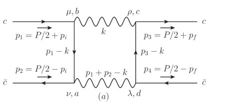
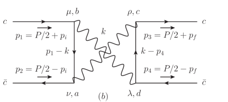
Figure 1: The Feynman diagrams for $q\overline{q}\rightarrow 2g\rightarrow q\overline{q}$.

When one take the quark anti-quark pairs as off shell, the corresponding Green function is a part of the interaction kernel of the Bethe-Salpeter equation which plays the role like the potential in the non-relativistic quantum mechanics. The direct calculation of the corresponding Green function is a little tedious and there is no analytic expression in the full complex plane of momenta. Two methods are usually used to simplify the calculation. The first one is to project the quark anti-quark pairs to a special ${}^{2s+1}L_{J}$ state which is described as Fig. 2 and the second one is to study the asymptotic behavior of this Green function which means to expand the expression on some small variables.

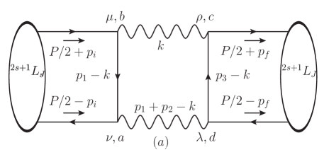
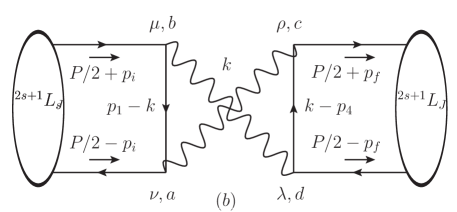
Figure 2: The Feynman diagrams for $q\overline{q}\rightarrow 2g\rightarrow q\overline{q}$ in ${}^{2s+1}L_{J}$ channel.

In the center mass frame, the momenta can be chosen as following.

$$p_{1} \triangleq \frac{1}{2}P+p_{i},~{}~{}~{}~{}p_{2}\triangleq\frac{1}{2}P-p_{i},$$

$$p_{3} \triangleq \frac{1}{2}P+p_{f},~{}~{}~{}~{}p_{4}\triangleq\frac{1}{2}P-p_{f},$$ (1)

with $P\triangleq(\sqrt{s},0,0,0)$. In the general case, there are six independent Lorentz invariant variables in the interaction kernel: $P^{2},~{}P\cdot p_{i},~{}P\cdot p_{f},~{}p_{i}^{2},~{}p_{f}^{2}$. For simplicity, we limit our discussion in the case with $P\cdot p_{i}=P\cdot p_{f}=0$. This region is corresponding to the instantaneous approximation for the Bethe-Salpeter equation which means the contributions from the relative energy of the quark anti-quark pair in the bound states is neglected. This property naturally appears when the initial and final quark anti-quark pairs are taken as on shell. Such choice of the momenta leaves the number of the independent Lorentz invariant variables to 4 and we can define $p_{i}\triangleq(0,\textbf{p}_{i}),p_{f}\triangleq(0,\textbf{p}_{f})$. This is different with the on shell case where there are only two independent Lorentz invariant variables $P^{2}=s\triangleq 4m^{2}+4p^{2}$ and $p_{i}\cdot p_{f}$ with $m$ the mass of quark. For the heavy quark anti-quark pair system, we can take $p_{i}^{2}/m^{2},~{}p_{f}^{2}/m^{2},~{}p_{i}\cdot p_{f}/m^{2}$ as small variables and leave $s$ as a free variable at first.

To project the quark anti-quark pairs to a special ${}^{1}S_{0}$ state, we use the same project matrix as the on shell case project-operator-1 ; project-operator-2 ; project-operator-3 where one has

$$\sum\overline{v}(p_{2},s_{2})Tu(p_{1},s_{1})<\frac{1}{2}s_{1};\frac{1}{2}s_{2}|00> \triangleq \textrm{Tr}[T.\Pi_{ini}],$$

$$\sum\overline{u}(p_{3},s_{3})Tv(p_{4},s_{4})<\frac{1}{2}s_{3};\frac{1}{2}s_{4}|00> \triangleq \textrm{Tr}[T.\Pi_{fin}],$$ (2)

where the Clebsch-Gordan coefficients are the standard ones as Ref. project-operator-2 and the Dirac spinors are normalized as $u^{+}u=v^{+}v=1$ whose expressions are written as

$$u(p_{1},s_{1}) \triangleq \frac{p_{\!}\!\!/_{1}+m}{\sqrt{E_{1}(E_{1}+m)}}\begin{pmatrix}\xi^{s_{1}}\\ 0\end{pmatrix},$$

$$v(p_{2},s_{2}) \triangleq \frac{-p_{\!}\!\!/_{2}+m}{\sqrt{E_{2}(E_{2}+m)}}\begin{pmatrix}0\\ \eta^{s_{2}}\end{pmatrix},$$ (3)

with $E_{1,2}\triangleq\sqrt{\textbf{p}_{1,2}^{2}+m^{2}}$, $\xi^{1/2}=(1,0)^{T}$, $\xi^{-1/2}=(0,1)^{T}$, $\eta^{1/2}=(0,1)^{T}$ and $\eta^{-1/2}=(-1,0)^{T}$. This results in the following expressions.

$$\Pi_{ini} = \frac{1}{8\sqrt{2}E_{i}^{2}(E_{i}+m)}(p\!\!\!/_{1}+m)(\sqrt{s}+P\!\!\!/)\gamma^{5}(-p\!\!\!/_{2}+m),$$

$$\Pi_{fin} = -\frac{1}{8\sqrt{2}E_{f}^{2}(E_{f}+m)}(-p\!\!\!/_{4}+m)\gamma^{5}(\sqrt{s}+P\!\!\!/)(p\!\!\!/_{3}+m),$$ (4)

where $E_{i,f}\triangleq\sqrt{\textbf{p}_{i,f}^{2}+m^{2}}$ and one should note that there is a minus in the expression of $\Pi_{fin}$.

We want to point out, the form of such project matrix is just for simplicity in our calculation. In principle the project matrix should be deduced from the Bethe-Salpeter equation and in the ultra non-relativistical limit the above expressions are expected to be true. In this work, we do not go to discuss the detail of this project matrix but just take the same form as the references.

Using the above project method, the interaction kernel in ${}^{1}S_{0}$ state can be expressed as the following.

$$G^{(a)}(^{1}S_{0}) = -ic_{f}^{(2g)}\int\frac{d^{D}k}{(2\pi)^{4}}\textrm{Tr}[T_{1}\cdot\Pi_{ini}]\textrm{Tr}[T_{2}\cdot\Pi_{fin}]D_{\mu\rho}(k)D_{\nu\lambda}(p_{1}+p_{2}-k),$$

$$G^{(b)}(^{1}S_{0}) = -ic_{f}^{(2g)}\int\frac{d^{D}k}{(2\pi)^{4}}\textrm{Tr}[T_{1}\cdot\Pi_{ini}]\textrm{Tr}[T_{3}\cdot\Pi_{fin}]D_{\mu\lambda}(k)D_{\nu\rho}(p_{1}+p_{2}-k),$$ (5)

where the color factor $c_{f}^{(2g)}$ is

$$c_{f}^{(2g)} = (\frac{\delta_{ij}}{\sqrt{N_{c}}}T_{a}^{jm}T_{b}^{mi})(\frac{\delta_{i^{\prime}j^{\prime}}}{\sqrt{N_{c}}}T_{c}^{j^{\prime}m^{\prime}}T_{d}^{m^{\prime}i^{\prime}})\delta_{ad}\delta_{bc}$$ (6)

$$= \frac{C_{A}C_{F}}{2N_{c}}=\frac{N_{c}^{2}-1}{4N_{c}}=\frac{2}{3},$$

and the hard kernel $T_{i}$ are

$$T_{1} = (-ig_{s}\gamma^{\nu})\cdot S_{F}(p_{1}-k)\cdot(-ig_{s}\gamma^{\mu}),$$

$$T_{2} = (-ig_{s}\gamma^{\rho})\cdot S_{F}(p_{3}-k)\cdot(-ig_{s}\gamma^{\lambda}),$$

$$T_{3} = (-ig_{s}\gamma^{\rho})\cdot S_{F}(k-p_{4})\cdot(-ig_{s}\gamma^{\lambda}),$$ (7)

with

$$S_{F}(q) = \frac{i(q\!\!\!/+m)}{q^{2}-{m}^{2}+i\epsilon},$$

$$D_{\mu\rho}(q) = \frac{-i}{q^{2}+i\epsilon}(g_{\mu\rho}-\xi\frac{q_{\mu}q_{\rho}}{q^{2}}).$$ (8)

For the on shell quark anti-quark pairs one has $(P/2\pm p_{i})^{2}=(P/2\pm p_{f})^{2}=m^{2}$ and these conditions lead to the denominators of the integrands in Eq. (5) include terms like $k^{2}-(P-2p_{i,f})\cdot k+i\epsilon$. This situation leads to the expansion on $p_{i,f}$ and the integration of the loop momentum un-commutative when one goes to estimate the asymptotic behavior of the expression. In this case, one can separate the loop integration into hard part and other parts using the region method region-methos . For the off shell quark anti-quark pairs, $(P^{2}/4-m^{2})$ is taken as a free finite quantity and one can commutate the expansion and the integration of the loop momentum safely.

III The analytic results for the asymptotic behavior

In our calculation, we at first use the package Feyncalc FeynCalc to do the trace of Dirac matrixes in $D$-dimension as Ref. JiaYu2011 , then expand the expression on the variables $p_{i}^{2},~{}p_{f}^{2},~{}p_{i}\cdot p_{f}$ to a special order. This expansion is equivalent to expand the expression on the four momenta $p_{i}$ and $p_{f}$ directly. After the expansion, we use the tensor decomposition to re-expressed the loop integrations as following.

$$\int_{k}\frac{(p_{i}\cdot k)^{6}}{k^{2}(P-k)^{2}((P/2-k)^{2}-m^{2})^{n}} = \int_{k}\frac{-15[k^{2}s-(k\cdot P)^{2}]^{3}|\textbf{p}_{i}|^{6}}{(D+3)(D^{2}-1)s^{3}k^{2}(P-k)^{2}((P/2-k)^{2}-m^{2})^{n}},$$

$$\int_{k}\frac{(p_{i}\cdot k)^{4}}{k^{2}(P-k)^{2}((P/2-k)^{2}-m^{2})^{n}} = \int_{k}\frac{3[(k\cdot P)^{2}-k^{2}s]^{2}|\textbf{p}_{i}|^{4}}{(D^{2}-1)s^{2}k^{2}(P-k)^{2}((P/2-k)^{2}-m^{2})^{n}},$$

$$\int_{k}\frac{(p_{i}\cdot k)^{2}}{k^{2}(P-k)^{2}((P/2-k)^{2}-m^{2})^{n}} = \int_{k}\frac{[sk^{2}-(k\cdot P)^{2}]|\textbf{p}_{i}|^{2}}{(1-D)sk^{2}(P-k)^{2}((P/2-k)^{2}-m^{2})^{n}},$$

$$\int_{k}\frac{(p_{i}\cdot k)^{4}\ (p_{f}\cdot k)^{2}}{k^{2}(P-k)^{2}((P/2-k)^{2}-m^{2})^{n}} = \int_{k}\frac{-3(4\beta^{2}+1)[k^{2}s-(k\cdot P)^{2}]^{3}|\textbf{p}_{i}|^{4}|\textbf{p}_{f}|^{2}}{(D+3)(D^{2}-1)s^{3}k^{2}(P-k)^{2}((P/2-k)^{2}-m^{2})^{n}}.$$

$$\int_{k}\frac{(p_{i}\cdot k)^{2}\ (p_{f}\cdot k)^{2}}{k^{2}(P-k)^{2}((P/2-k)^{2}-m^{2})^{n}} = \int_{k}\frac{(2\beta^{2}+1)[(k\cdot P)^{2}-k^{2}s]^{2}|\textbf{p}_{i}|^{2}|\textbf{p}_{f}|^{2}}{(D^{2}-1)s^{2}k^{2}(P-k)^{2}((P/2-k)^{2}-m^{2})^{n}},$$ (9)

with $\beta\triangleq\textbf{p}_{i}.\textbf{p}_{f}/|\textbf{p}_{i}||\textbf{p}_{f}|$ and $\int_{k}\triangleq\int d^{D}k$. After the expansion and the tensor decomposition, for simplicity we directly use the package FIESTA FIESTA to do the sector decomposition with $i\epsilon$ kept in the propagators and output the date base for integration, then use Mathematica to do the analytic integration.

In the practical calculation, we expand the expressions on $|\textbf{p}_{i,f}|$ to order 6. The gauge parameter $\xi$ is also kept in the practical calculation and we find the result is not dependent on $\xi$ which means the result is gauge independent although the momentum $P/2\pm p_{i,f}$ are not on shell. The direct numerical calculation is also used to check the analytic result.

After the loop integration, we apply the following property to reduce the variables since we only care for the matrix element of the interaction kernel between the ${}^{1}S_{0}$ states.

$$\int d\Omega_{\textbf{p}_{i}}d\Omega_{\textbf{p}_{f}}\textbf{p}_{i}\cdot\textbf{p}_{f} = 0,$$

$$\int d\Omega_{\textbf{p}_{i}}d\Omega_{\textbf{p}_{f}}(\textbf{p}_{i}\cdot\textbf{p}_{f})^{2} = \frac{1}{3}|\textbf{p}_{i}||\textbf{p}_{f}|\int d\Omega_{\textbf{p}_{i}}d\Omega_{\textbf{p}_{f}}.$$ (10)

The high terms like $(\textbf{p}_{i}\cdot\textbf{p}_{f})^{4}$ are not appeared in the expression and we need not care for them.

Eq.(10) means we can replace the terms $(\textbf{p}_{i}\cdot\textbf{p}_{f})^{2}$ and $(\textbf{p}_{i}\cdot\textbf{p}_{f})$ by $\frac{1}{3}|\textbf{p}_{i}||\textbf{p}_{f}|$ and $0$ in our discussion. After such replacement, the final result can be expressed as

$$\overline{G}^{(a+b)}(^{1}S_{0})\Big{|}_{|\textbf{p}_{i,f}|} = c_{f}^{(2g)}\alpha_{s}^{2}\Big{[}\frac{1}{m^{2}}c_{0}^{full}+\frac{1}{m^{4}}c_{2}^{full}+\frac{1}{m^{6}}c_{4}^{full}+\frac{1}{m^{8}}c_{6}^{full}+\textrm{higher order}\Big{]},$$ (11)

where $\overline{G}$ refers to the result of $G$ after the replacement, the subindexes $|\textbf{p}_{i,f}|$ mean to expand the expression on $|\textbf{p}_{i,f}|$ and $c^{full}_{i}$ are some functions on $p^{2}$ with corresponding orders of $|\textbf{p}_{i,f}|$. The manifest expressions of $c_{i}^{full}$ are a little complex and we list them in the Appendix. To compare the results with those given in NRQCD, we further expand the above results on $p^{2}$ and rearrange the results as

$$\overline{G}^{(a+b)}(^{1}S_{0})\Big{|}_{|\textbf{p}_{i}|,|\textbf{p}_{f}|,p^{2}} = c_{f}^{(2g)}\alpha_{s}^{2}\Big{[}\frac{1}{m^{2}}c_{0}+\frac{1}{m^{4}}c_{2}+\frac{1}{m^{6}}c_{4}+\frac{1}{m^{8}}c_{6}+\textrm{higher order}\Big{]},$$ (12)

where $c_{i}$ are the combinations of terms with corresponding orders of $\textbf{p}_{i,f}^{2}$ and $p^{2}$. For $p^{2}>0$ $c_{i}$ are expressed as

$$\textrm{Im}[c_{0}] = 2\pi,$$

$$\textrm{Im}[c_{2}] = -\frac{2\pi}{3}\Big{[}5(|\textbf{p}_{f}|^{2}+|\textbf{p}_{i}|^{2})-6p^{2}\Big{]},$$

$$\textrm{Im}[c_{4}] = \frac{\pi}{360}\Big{[}1059(|\textbf{p}_{i}|^{4}|+\textbf{p}_{f}|^{4})+1640|\textbf{p}_{i}|^{2}|\textbf{p}_{f}|^{2}-1110(|\textbf{p}_{i}|^{2}|+|\textbf{p}_{f}|^{2})p^{2}-450p^{4}\Big{]},$$

$$\textrm{Im}[c_{6}] = -\frac{\pi}{10080}\Big{[}39435(|\textbf{p}_{i}|^{6}+|\textbf{p}_{f}|^{6})+42700(|\textbf{p}_{f}|^{4}|\textbf{p}_{f}|^{2}|+\textbf{p}_{f}|^{2}|\textbf{p}_{f}|^{4})$$

$$~{}~{}~{}~{}~{}~{}~{}-55986(|\textbf{p}_{f}|^{4}+|\textbf{p}_{f}|^{4}|)p^{2}-21840|\textbf{p}_{i}|^{2}|\textbf{p}_{f}|^{2}p^{2}$$

$$~{}~{}~{}~{}~{}~{}~{}+4935(|\textbf{p}_{f}|^{2}+|\textbf{p}_{f}|^{2})p^{4}-7560p^{6})\Big{]},$$

and

$$\textrm{Re}[c_{0}] = 4(1-\log 2),$$

$$\textrm{Re}[c_{2}] = \frac{1}{3}\Big{[}(20\log 2-13)(|\textbf{p}_{i}|^{2}+|\textbf{p}_{f}|^{2})+6(1-4\log 2)p^{2}\Big{]},$$

$$\textrm{Re}[c_{4}] = \frac{1}{180}\Big{[}(180\log r_{p^{2}}+1131-1419\log 2)(|\textbf{p}_{i}|^{4}+|\textbf{p}_{f}|^{4})$$

$$~{}~{}~{}~{}~{}+\big{[}180\log r_{p^{2}}+1010-2000\log 2)|\textbf{p}_{i}|^{2}|\textbf{p}_{f}|^{2}$$

$$~{}~{}~{}~{}~{}+(-540\log r_{p^{2}}-510+2190\log 2)(|\textbf{p}_{i}|^{2}+|\textbf{p}_{f}|^{2})p^{2}$$

$$~{}~{}~{}~{}~{}+(540\log r_{p^{2}}-450-630\log 2)p^{4}$$

$$~{}~{}~{}~{}~{}-\frac{45(|\textbf{p}_{f}|^{6}+|\textbf{p}_{f}|^{4}|\textbf{p}_{i}|^{2}+|\textbf{p}_{f}|^{2}|\textbf{p}_{i}|^{4}+|\textbf{p}_{i}|^{6})}{p^{2}}\Big{]},$$

$$\textrm{Re}[c_{6}] = \frac{1}{5040}\Big{[}(1680\log r_{p^{2}}+25968-42795\log 2)(|\textbf{p}_{i}|^{6}+|\textbf{p}_{f}|^{6})$$ (14)

$$~{}~{}~{}~{}~{}+(11760\log r_{p^{2}}+40047-66220\log 2)(|\textbf{p}_{i}|^{4}|\textbf{p}_{f}|^{2}+|\textbf{p}_{i}|^{4}|\textbf{p}_{f}|^{2})$$

$$~{}~{}~{}~{}~{}+(-6720\log r_{p^{2}}-5040+69426\log 2)(|\textbf{p}_{i}|^{4}+|\textbf{p}_{f}|^{4})p^{2}$$

$$~{}~{}~{}~{}~{}+(-35280\log r_{p^{2}}-16380+92400\log 2)|\textbf{p}_{i}|^{2}|\textbf{p}_{f}|^{2}p^{2}$$

$$~{}~{}~{}~{}~{}+(8400\log r_{p^{2}}-21735-21735\log 2)(|\textbf{p}_{i}|^{2}+|\textbf{p}_{f}|^{2})p^{4}$$

$$~{}~{}~{}~{}~{}+(5040\log r_{p^{2}}+2100-1680\log 2)p^{6}\Big{]},$$

where $r_{p^{2}}\triangleq p^{2}/m^{2}$ and is assumed to be larger than 0 in the above expressions. For the $r_{p^{2}}<0$ case, the term $\log r_{p^{2}}$ should be taken as $\log(r_{p^{2}}+i\epsilon)$ with $\epsilon=0^{+}$ and it gives an additional contribution to the imagine part of the coefficients. This analytic continuation is also checked by the direct calculation with $r_{p^{2}}<0$. For convenient we also list the expressions with $p^{2}<0$ which can be used in the positronium system.

$$\textrm{Im}[c_{0}^{(p^{2}<0)}] = \textrm{Im}[c_{0}],$$

$$\textrm{Im}[c_{2}^{(p^{2}<0)}] = \textrm{Im}[c_{2}],$$

$$\textrm{Im}[c_{4}^{(p^{2}<0)}] = \frac{\pi}{360}\Big{[}1419(|\textbf{p}_{i}|^{4}|+\textbf{p}_{f}|^{4})+2000|\textbf{p}_{i}|^{2}|\textbf{p}_{f}|^{2}-2190(|\textbf{p}_{i}|^{2}|+|\textbf{p}_{f}|^{2})p^{2}+630p^{4}\Big{]},$$

$$\textrm{Im}[c_{6}^{(p^{2}<0)}] = -\frac{\pi}{10080}\Big{[}42795(|\textbf{p}_{i}|^{6}+|\textbf{p}_{f}|^{6})+66220(|\textbf{p}_{f}|^{4}|\textbf{p}_{f}|^{2}|+\textbf{p}_{f}|^{2}|\textbf{p}_{f}|^{4})$$ (15)

$$~{}~{}~{}~{}~{}~{}~{}-69426(|\textbf{p}_{f}|^{4}+|\textbf{p}_{f}|^{4}|)p^{2}-92400|\textbf{p}_{i}|^{2}|\textbf{p}_{f}|^{2}p^{2}$$

$$~{}~{}~{}~{}~{}~{}~{}+21735(|\textbf{p}_{f}|^{2}+|\textbf{p}_{f}|^{2})p^{4}+2520p^{6})\Big{]}.$$

The real parts of the expressions for $p^{2}<0$ are same with the expressions with $p^{2}>0$ by changing $r_{p}^{2}$ to $-r_{p}^{2}$.

Using the above expressions and the quasi potential method, one can directly get the corresponding non-relativistic potential in the LO-$\alpha_{s}$. In the momentums space it is expressed as

$$V_{eff}(^{1}S_{0}) = -G^{(a+b)}(^{1}S_{0}),$$ (16)

since we have normalized the Dirac spinors as $u^{+}u=v^{+}v=1$.

Taking this effective potential as a perturbative interaction comparing with the non-perturbative potential in the quark model. The corresponding energy shift in the leading order can be got directly as

$$\Delta E(s) = <V_{eff}^{{}^{1}S_{0}}>$$ (17)

$$= \int d^{3}\textbf{p}_{i}d^{3}\textbf{p}_{f}\Phi^{*}(\textbf{p}_{f})V_{eff}(^{1}S_{0},p_{i}^{2},p_{f}^{2},p_{i}\cdot p_{f},s)\Phi(\textbf{p}_{i}),$$

where $\Phi(\textbf{p}_{i,f})\triangleq\phi(|\textbf{p}_{i,f}|)Y_{00}$ are the wave functions of the ${}^{1}S_{0}$ states in the momentum space normalized as $\int d^{3}\textbf{p}\Phi^{*}(\textbf{p})\Phi(\textbf{p})=1$.

Corresponding, the result after the expansion and the integration is expressed as

$$\Delta E(s)\big{|}_{|\textbf{p}_{i}|,|\textbf{p}_{f}|} = -2\pi^{3}c_{f}^{(2g)}\alpha_{s}^{2}\Big{[}\frac{c_{01}^{full}}{m^{2}}\psi(0)^{2}-\frac{c_{21}^{full}}{m^{4}}2\psi^{(2)}(0)\psi(0)+\frac{c_{41}^{full}}{m^{6}}2\psi^{(4)}(0)\psi(0)$$ (18)

$$~{}~{}+\frac{c_{42}^{full}}{m^{6}}\psi^{(2)}(0)^{2}-\frac{c_{61}^{full}}{m^{8}}2\psi^{(6)}(0)\psi(0)-\frac{c_{62}^{full}}{m^{8}}2\psi^{(2)}(0)\psi^{(4)}(0)\Big{]},$$

where the coefficients can be found in the Appendix and $\psi^{(n)}(0)$ are defined as

$$\psi^{(n)}(0) \triangleq \frac{(-i)^{n}}{(2\pi)^{3/2}}\int|\textbf{p}|^{n}\Phi(\textbf{p})d^{3}\textbf{p},$$ (19)

with $n$ even. $\psi^{(n)}(0)$ are corresponding to the values of the $n$-th derivative of the wave functions in the coordinate space at $r=0$ since

$$\Phi(\textbf{p}) = \int\frac{1}{(2\pi)^{3/2}}e^{-i\textbf{p}\cdot\textbf{r}}\psi(\textbf{r})d^{3}\textbf{r}.$$ (20)

One should note that the angle part $Y_{00}$ is included in the wave function $\psi(\textbf{r})$.

Furthermore, one can expand the result on $p^{2}$ which gives

$$\Delta E(s)\big{|}_{|\textbf{p}_{i}|,|\textbf{p}_{f}|,p^{2}} = -2\pi^{3}c_{f}^{(2g)}\alpha_{s}^{2}\Big{[}\frac{c_{0}}{m^{2}}\psi(0)^{2}+\textrm{higher terms}\Big{]}.$$ (21)

Physically, the imagine part of $\Delta E(s)$ is corresponding to the decay width of a state as $\Gamma=-2\textrm{Im}[\Delta E(s)]$ with $\sqrt{s}=M_{{}^{1}S_{0}}$ and the real part of $\Delta E(s)$ is corresponding to the mass shift due to the two-gluon annihilation in the leading order.

Eq. (18) can also be directly used to estimate the decay widths of $\eta_{c,b}\rightarrow 2\gamma$, the mass shifts and decay widths of positronium in ${}^{1}S_{0}$ states due to the annihilation effect $e^{+}e^{-}\rightarrow 2\gamma$. For $\eta_{c,b}\rightarrow 2\gamma$, we should replace the factor $c_{f}^{(2g)}\alpha_{s}^{2}$ by $c_{f}^{(2\gamma)}Q_{c,b}^{4}\alpha_{QED}^{2}$ with $c_{f}^{(2\gamma)}=3$ and $Q_{b,c}$ the electric charges of $b,c$ quarks. For positronium, we should replace the factor $c_{f}^{(2g)}\alpha_{s}^{2}$ by $\alpha_{QED}^{2}$. Since in the positronium case one has $r_{p^{2}}<0$ or $r_{s}\triangleq\sqrt{s}/2m<1$, the corresponding $\textrm{Im}[c_{i}^{full}]$ and $\textrm{Re}[c_{i}^{full}]$ should be re-written by changing $\log(r_{s}^{2}-1)$ to $\log(r_{s}^{2}-1+i\epsilon)$ like Eq. (15).

IV comparison with the results of NRQCD in LO-$\alpha_{s}$

To compare the above results with the corresponding results in NRQCD in LO-$\alpha_{s}$, we can apply the on shell constrain conditions to the coefficients $c_{i}$. The on shell constrain conditions means $|\textbf{p}_{i}|^{2}=|\textbf{p}_{f}|^{2}=-p_{i}^{2}=-p_{f}^{2}=p^{2}$ which leads to the following results.

$$\textrm{Im}[c_{0}^{(on)}] = 2\pi,$$

$$\textrm{Im}[c_{2}^{(on)}] = -\frac{8\pi}{3}|\textbf{p}_{i}|^{2},$$

$$\textrm{Im}[c_{4}^{(on)}] = \frac{136\pi}{45}|\textbf{p}_{i}|^{4},$$

$$\textrm{Im}[c_{6}^{(on)}] = -\frac{1024\pi}{315}|\textbf{p}_{i}|^{6},$$ (22)

where the index $(on)$ refers to the results after applying the on shell conditions to $c_{i}$.

Comparing these results to the decay width of $\Gamma(\eta_{c}\rightarrow 2\gamma)$ in NRQCD project-operator-2 which expressed as

$$\Gamma(H(^{1}S_{0})\rightarrow\gamma\gamma)$$

$$= \frac{2\alpha_{QED}^{2}Q^{4}\pi}{m^{2}}\langle H(^{1}S_{0})|\mathcal{O}_{\textrm{em}}(^{1}S_{0})|H(^{1}S_{0})\rangle-\frac{8\alpha_{QED}^{2}Q^{4}\pi}{3m^{4}}\langle H(^{1}S_{0})|\mathcal{P}_{\textrm{em}}(^{1}S_{0})|H(^{1}S_{0})\rangle$$

$$+\frac{20\alpha_{QED}^{2}Q^{4}\pi}{9m^{6}}\langle H(^{1}S_{0})|\mathcal{Q}^{\prime}_{\textrm{em}}(^{1}S_{0})|H(^{1}S_{0})\rangle+\frac{4\alpha_{QED}^{2}Q^{4}\pi}{5m^{6}}\langle H(^{1}S_{0})|\mathcal{Q}^{\prime\prime}_{\textrm{em}}(^{1}S_{0})|H(^{1}S_{0})\rangle,$$

with

$$\mathcal{O}_{\textrm{em}}(^{1}S_{0}) = \psi^{{\dagger}}\chi|0\rangle\langle 0|\chi^{{\dagger}}\psi,$$

$$\mathcal{P}_{\textrm{em}}(^{1}S_{0}) = \frac{1}{2}\psi^{{\dagger}}(-\frac{i}{2}\overleftrightarrow{D})^{2}\chi|0\rangle\langle 0|\chi^{{\dagger}}\psi+\textrm{H.c.},$$

$$\mathcal{Q^{\prime}}_{\textrm{em}}(^{1}S_{0}) = \psi^{{\dagger}}(-\frac{i}{2}\overleftrightarrow{D})^{2}\chi|0\rangle\langle 0|\chi^{{\dagger}}(-\frac{i}{2}\overleftrightarrow{D})^{2}\psi,$$

$$\mathcal{Q^{\prime\prime}}_{\textrm{em}}(^{1}S_{0}) = \frac{1}{2}\psi^{{\dagger}}(-\frac{i}{2}\overleftrightarrow{D})^{4}\chi|0\rangle\langle 0|\chi^{{\dagger}}\psi+\textrm{H.c.}.$$ (24)

One can find the $\textbf{p}_{i,f}$ in Eq. (22) are correcponding to the operaor $-\frac{i}{2}\overleftrightarrow{D}$ in Eq. (24), $\textrm{Im}[c^{(on)}_{0,2}]$ are same with the coefficients of the 1st, 2nd terms and $\textrm{Im}[c^{(on)}_{4}]$ is same with the sum of the coefficients of 3rd and 4th terms of Eq.(LABEL:NQRCD) except a global factor $\alpha_{QED}^{2}Q^{4}$ and a normalized factor $1/m^{n}$. This is natural since we just take $s$ as a free variable at first and then apply the on shell conditions after the loop integration, the results should go back to NRQCD results which takes the on shell conditions directly. The coefficient $\textrm{Im}[c^{(on)}_{6}]$ is corresponding to the sum of coefficients in NRQCD in order $v^{6}$ JiaYu2011 . In our calculation we take the quantities $p^{2},|\textbf{p}_{i}|,|\textbf{p}_{f}|,\textbf{p}_{i}\cdot\textbf{p}_{f}$ as independent variables at first and then using the on shell conditions $p^{2}=|\textbf{p}_{i}|^{2}=|\textbf{p}_{f}|^{2}$, this means that we can not distinguish $|\textbf{p}_{i}|$ and $|\textbf{p}_{f}|$ when applying the on shell conditions and we can only give the sum of the corresponding NRQCD coefficients. The real part of $c_{i}^{(on)}$ can also be got easily from Eq.(14) as following.

$$\textrm{Re}[c_{0}^{(on)}] = 4(1-\log 2),$$

$$\textrm{Re}[c_{2}^{(on)}] = \frac{4}{3}|\textbf{p}_{i}|^{2}(4\log 2-5),$$

$$\textrm{Re}[c_{4}^{(on)}] = \frac{1}{90}|\textbf{p}_{i}|^{4}(811-544\log 2),$$

$$\textrm{Re}[c_{6}^{(on)}] = \frac{1}{630}|\textbf{p}_{i}|^{6}(4096\log 2-8025),$$ (25)

where the result $\textrm{Re}[c_{0}^{(on)}]$ is same with that given in the reference Real-part-refs . We want to point out that for positronium where $p^{2}<0,r_{s}<1$, we do not suggest use the Eq. (22,25) but suggest to use the corresponding expressions with $p^{2}<0$.

V The numerical result and conclusion

For the visualization, we list some numerical results in this section. In NRQCD, the contribution to the decay width in the LO-$v$ and LO-$\alpha_{s}$ is determined by the coefficient $c_{0}$ and the wave function at zero point $\psi(0)$. In our calculation, we expand the expression only on $|\textbf{p}_{i}|,|\textbf{p}_{f}|$ and $\textbf{p}_{i}\cdot\textbf{p}_{f}$ and do not take the on shell conditions to fix $s$. This results in the corresponding decay width is also dependent on $s$. The ratio $\textrm{Im}[c_{0}^{full}]/\textrm{Im}[c_{0}]$ reflects the corresponding correction to the decay width in NRQCD in leading order due to the off shell effect. Such correction is not dependent on the non-perturbative parameter $\psi(0)$ but only dependent on the ratio $r_{s}$. The corresponding numerical results are presented in the left panel of Fig. 3.

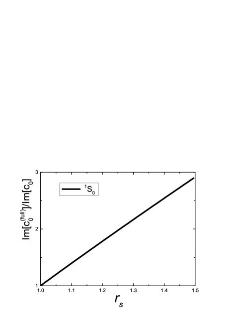
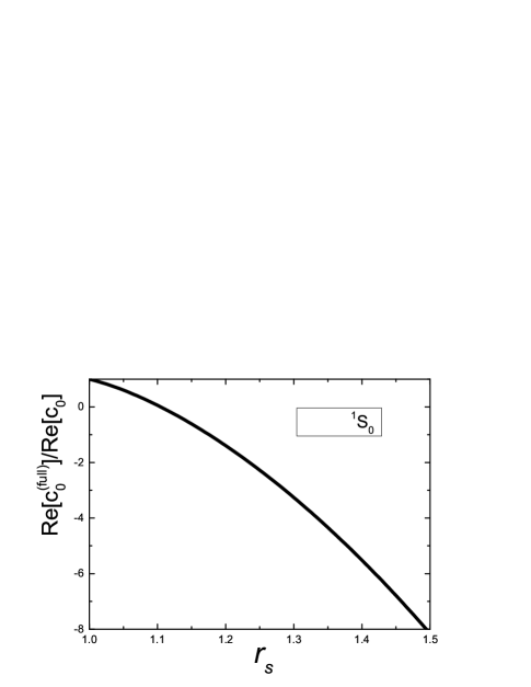
Figure 3: The numerical results for the corrections to the decay width and the mass shift for ${}^{1}S_{0}$ state in the leading order of $\alpha_{s}$ and $v$ where $r_{s}\triangleq\sqrt{s}/2m$.

In the right panel of Fig. 3, we also present the similar correction to the real part of the coefficient. The ratio $\textrm{Re}[c_{0}^{full}]/\textrm{Re}[c_{0}]$ reflects the correction to the mass shift due to the off shell effect. In the positronium case, the bound energies of the physical bound states are very small relative to the mass of electron which means the ratios $|r_{s}|=(2m-\Delta E)/2m$ are very close to 1 and the corrections are very small. In the charmonium case, the bound energies of the physical states are not so small comparing with the quark mass and the $r_{s}$ for the real physical states are also not small. For example, if we take the mass of $c$ quark as a constant, then the relative ratio $r_{s}(\eta_{c}(2S))/r_{s}(\eta_{c}(1S))=M_{\eta_{c}(2S)}/M_{\eta_{c}(1S)}=1.22$ which is not a small value. This means the correction is not small.

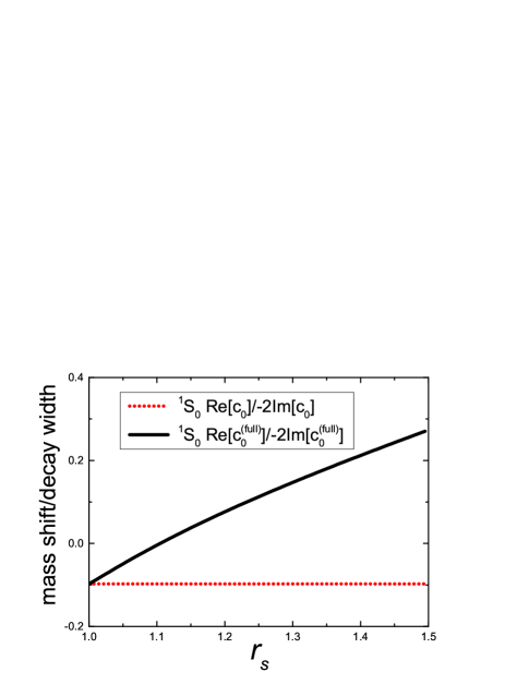
Figure 4: The numerical results for the ratio of the mass shift and the decay width for ${}^{1}S_{0}$ state in the leading order of $\alpha_{s}$ and $v$ .

In Fig. 4, the ratios $\textrm{Re}[c_{0}^{full}]/-2\textrm{Im}[c_{0}^{full}]$ and $\textrm{Re}[c^{(on)}_{0}]/-2\textrm{Im}[c^{(on)}_{0}]$ are presented. These ratios reflect the relation between the mass shifts and the decay widths. If one assumes the LO gives the most of the contribution, one can use the experimental decay width to estimate the mass shift. For the heavy quarknia, if we take the approximation $r_{s}(\eta_{c})\approx 1$ and $r_{s}(\eta_{b})\approx 1$ then the corrections to the mass shifts are about $-(1-\log 2)/\pi\Gamma(\eta_{c})\approx-3.1$ MeV for $\eta_{c}$, $0.09\Gamma(\eta_{c}(2S))=1.0$ MeV for $\eta_{c}(2S)$, $-(1-\log 2)/\pi\Gamma(\eta_{b})\approx-6.1$ MeV for $\eta_{b}$ and $-0.04\Gamma(\eta_{b}(2S))$ for $\eta_{b}(2S)$. The interesting property is that the mass shifts are strong dependent on the mass or the binding energy of ${}^{1}S_{0}$ states. This means the corrections to the different ${}^{1}S_{0}$ states are very different and can not be subtracted or hidden in a unified way.

In summary, the non-relativistic asymptotic behavior of the transition $q\overline{q}\rightarrow 2g\rightarrow q\overline{q}$ in the ${}^{1}S_{0}$ channel is discussed. In our discussion, the momenta of the quarks and anti-quarks are not limited on mass shell after projecting the quark anti-quark pairs to ${}^{1}S_{0}$ state. We calculate the results by expanding the expression on the three-dimensional momenta of quarks and anti-quarks to order 6. The imagine part of the first 3 terms of our results after applying the on shell conditions can reproduce the non-relativistic QCD (NRQCD) results in leading order of $\alpha_{s}$. The real part of our results can be used to estimate the mass shift of ${}^{1}S_{0}$ heavy quark anti-quark system due to the $2g$ annihilation effect. The results can also be used to estimate the energy shifts of ${}^{1}S_{0}$ states of positronium.

VI Acknowledgments

The author Hai-Qing Zhou would like to thank Wen-Long Sang, Zhi-Yong Zhou and Dian-Yong Chen for their kind and helpful discussions. This work is supported by the National Natural Science Foundations of China under Grant No. 11375044.

VII Appendix

In this Appendix, the expressions for $c_{i}^{full}$ are listed.

$$c_{0}^{full} = c_{01}^{full},$$

$$c_{2}^{full} = (|\textbf{p}_{i}|^{2}+|\textbf{p}_{f}|^{2})c_{21}^{full},$$

$$c_{4}^{full} = (|\textbf{p}_{i}|^{4}+|\textbf{p}_{f}|^{4})c_{41}^{full}+|\textbf{p}_{i}|^{2}|\textbf{p}_{f}|^{2}c_{42}^{full},$$

$$c_{6}^{full} = (|\textbf{p}_{i}|^{6}+|\textbf{p}_{f}|^{6})c_{61}^{full}+(|\textbf{p}_{i}|^{4}|\textbf{p}_{f}|^{2}+|\textbf{p}_{i}|^{2}|\textbf{p}_{f}|^{4})c_{62}^{full},$$ (26)

with

$$\textrm{Im}[c_{01}^{full}] = \frac{\pi\alpha^{2}(\text{rs}+1)^{4}(3r_{s}^{4}-1)}{4\text{mc}^{2}r_{s}^{2}(r_{s}^{2}+1)^{2}},$$ (27)

$$\textrm{Im}[c_{21}^{full}] = -\frac{\pi(r_{s}+1)^{2}}{48m^{4}r_{s}^{4}(r_{s}^{2}+1)^{4}}\Big{(}35r_{s}^{12}+94r_{s}^{11}+145r_{s}^{10}+100r_{s}^{9}+172r_{s}^{8}$$ (28)

$$~{}~{}+52r_{s}^{7}+36r_{s}^{6}-12r_{s}^{5}-31r_{s}^{4}+22r_{s}^{3}+3r_{s}^{2}+16r_{s}+8\Big{)},$$

$$\textrm{Im}[c_{41}^{full}] = \frac{\pi(r_{s}+1)^{2}}{240m^{6}r_{s}^{6}(r_{s}^{2}+1)^{6}}\Big{(}185r_{s}^{18}+520r_{s}^{17}+1139r_{s}^{16}+1518r_{s}^{15}+2566r_{s}^{14}$$ (29)

$$~{}~{}+2404r_{s}^{13}+2756r_{s}^{12}+888r_{s}^{11}+1329r_{s}^{10}+20r_{s}^{9}+15r_{s}^{8}-510r_{s}^{7}$$

$$~{}~{}-284r_{s}^{6}-504r_{s}^{5}-210r_{s}^{4}-296r_{s}^{3}-132r_{s}^{2}-72r_{s}-36\Big{)},$$

$$\textrm{Im}[c_{42}^{full}] = \frac{\pi}{576m^{6}r_{s}^{6}(r_{s}^{2}+1)^{6}}\Big{(}375r_{s}^{20}+2220r_{s}^{19}+6102r_{s}^{18}+11084r_{s}^{17}+16964r_{s}^{16}$$ (30)

$$~{}~{}+20820r_{s}^{15}+24114r_{s}^{14}+19988r_{s}^{13}+18494r_{s}^{12}+11892r_{s}^{11}+10810r_{s}^{10}$$

$$~{}~{}+7060r_{s}^{9}+5484r_{s}^{8}+5772r_{s}^{7}+3230r_{s}^{6}+2892r_{s}^{5}+843r_{s}^{4}+128r_{s}^{3}$$

$$~{}~{}-96r_{s}^{2}-192r_{s}-48\Big{)},$$

$$\textrm{Im}[c_{61}^{full}] = -\frac{\pi(r_{s}+1)^{2}}{26880m^{8}r_{s}^{8}(r_{s}^{2}+1)^{8}}\Big{(}21595r_{s}^{24}+61670r_{s}^{23}+176925r_{s}^{22}+300580r_{s}^{21}$$ (31)

$$~{}~{}+590734r_{s}^{20}+710200r_{s}^{19}+1068266r_{s}^{18}+768220r_{s}^{17}+1099948r_{s}^{16}$$

$$~{}~{}+608700r_{s}^{15}+596964r_{s}^{14}+50540r_{s}^{13}+95578r_{s}^{12}+1960r_{s}^{11}-54698r_{s}^{10}$$

$$~{}~{}+106820r_{s}^{9}+10409r_{s}^{8}+177310r_{s}^{7}+69135r_{s}^{6}+128720r_{s}^{5}+57576r_{s}^{4}$$

$$~{}~{}+48480r_{s}^{3}+23088r_{s}^{2}+7680r_{s}+3840\Big{)},$$

$$\textrm{Im}[c_{62}^{full}] = -\frac{\pi}{2880m^{8}r_{s}^{8}\left(r_{s}^{2}+1\right)^{8}}\Big{(}1950r_{s}^{26}+12030r_{s}^{25}+36570r_{s}^{24}+82940r_{s}^{23}$$ (32)

$$~{}~{}+154123r_{s}^{22}+244280r_{s}^{21}+346088r_{s}^{20}+404804r_{s}^{19}+451148r_{s}^{18}$$

$$~{}~{}+403236r_{s}^{17}+389788r_{s}^{16}+252548r_{s}^{15}+208854r_{s}^{14}+107264r_{s}^{13}$$

$$~{}~{}+76392r_{s}^{12}+18460r_{s}^{11}-1386r_{s}^{10}-22594r_{s}^{9}-16038r_{s}^{8}-20096r_{s}^{7}$$

$$~{}~{}-6889r_{s}^{6}-4504r_{s}^{5}+416r_{s}^{4}+1824r_{s}^{3}+1032r_{s}^{2}+768r_{s}+192\Big{)}$$

$$\textrm{Re}[c_{01}^{full}] = -\frac{(r_{s}+1)^{4}}{4m^{2}r_{s}^{2}(r_{s}^{2}+1)^{2}}\Big{[}4r_{s}^{6}\log r_{s}+r_{s}^{6}(4\log 2-1)-2r_{s}^{4}-r_{s}^{2}$$ (33)

$$~{}~{}+(-2r_{s}^{6}+3r_{s}^{4}-1)\log(r_{s}^{2}-1)\Big{]},$$

$$\textrm{Re}[c_{21}^{full}] = \frac{(r_{s}+1)^{2}}{48m^{4}r_{s}^{4}(r_{s}^{2}+1)^{4}}\Big{\{}4(15r_{s}^{6}+30r_{s}^{5}+61r_{s}^{4}+52r_{s}^{3}+77r_{s}^{2}+54r_{s}+31)r_{s}^{8}\log r_{s}$$ (34)

$$~{}~{}-(r_{s}+1)^{2}(30r_{s}^{12}+57r_{s}^{10}-104r_{s}^{9}+160r_{s}^{8}-208r_{s}^{7}+146r_{s}^{6}-136r_{s}^{5}$$

$$~{}~{}+90r_{s}^{4}-32r_{s}^{3}+5r_{s}^{2}-8)\log(r_{s}^{2}-1)+r_{s}^{2}\Big{[}15r_{s}^{12}(4\log 2-1)$$

$$~{}~{}+30r_{s}^{11}(4\log 2-1)+r_{s}^{10}(244\log 2-85)+4r_{s}^{9}(52\log 2-31)$$

$$~{}~{}+14r_{s}^{8}(22\log 2-13)+8r_{s}^{7}(27\log 2-20)+2r_{s}^{6}(62\log 2-89)$$

$$~{}~{}-52r_{s}^{5}-67r_{s}^{4}+30r_{s}^{3}+7r_{s}^{2}+16r_{s}+8\Big{]}\Big{\}},$$

$$\textrm{Re}[c_{41}^{full}] = -\frac{(r_{s}+1)^{2}}{480m^{6}r_{s}^{6}(r_{s}^{2}+1)^{6}}\Big{\{}4(165r_{s}^{10}+330r_{s}^{9}+1025r_{s}^{8}+1220r_{s}^{7}+2482r_{s}^{6}$$ (35)

$$~{}~{}+2128r_{s}^{5}+3074r_{s}^{4}+1340r_{s}^{3}+1977r_{s}^{2}+870r_{s}+525)r_{s}^{10}\log r_{s}$$

$$~{}~{}+r_{s}^{2}\Big{[}165r_{s}^{18}(4\log 2-1)+330r_{s}^{17}(4\log 2-1)$$

$$~{}~{}+2r_{s}^{16}(2050\log 2-647)+r_{s}^{15}(4880\log 2-2018)$$

$$~{}~{}+r_{s}^{14}(9928\log 2-4215)+28r_{s}^{13}(304\log 2-165)$$

$$~{}~{}+4r_{s}^{12}(3074\log 2-1829)+20r_{s}^{11}(268\log 2-283)$$

$$~{}~{}+r_{s}^{10}(7908\log 2-7231)+6r_{s}^{9}(580\log 2-723)+6r_{s}^{8}(350\log 2-681)$$

$$~{}~{}-2442r_{s}^{7}-1433r_{s}^{6}-1352r_{s}^{5}-576r_{s}^{4}-664r_{s}^{3}-300r_{s}^{2}-144r_{s}-72\Big{]}$$

$$~{}~{}-2(165r_{s}^{20}+330r_{s}^{19}+840r_{s}^{18}+700r_{s}^{17}+1343r_{s}^{16}+610r_{s}^{15}+508r_{s}^{14}$$

$$~{}~{}-1064r_{s}^{13}-779r_{s}^{12}-18r_{s}^{11}-804r_{s}^{10}-20r_{s}^{9}-15r_{s}^{8}+510r_{s}^{7}+284r_{s}^{6}$$

$$~{}~{}+504r_{s}^{5}+210r_{s}^{4}+296r_{s}^{3}+132r_{s}^{2}+72r_{s}+36)\log(r_{s}^{2}-1)\Big{\}}$$

$$\textrm{Re}[c_{42}^{full}] = -\frac{1}{576m^{6}r_{s}^{6}(r_{s}^{2}+1)^{6}}\Big{\{}4(15r_{s}^{6}+30r_{s}^{5}+61r_{s}^{4}+52r_{s}^{3}+77r_{s}^{2}+54r_{s}+31)^{2}r_{s}^{10}\log r_{s}$$ (36)

$$~{}~{}+r_{s}^{2}\Big{[}225r_{s}^{20}(4\log 2-1)+900r_{s}^{19}(4\log 2-1)+8r_{s}^{18}(1365\log 2-382)$$

$$~{}~{}+4r_{s}^{17}(5220\log 2-1771)+4r_{s}^{16}(9151\log 2-3580)+4r_{s}^{15}(12584\log 2-5645)$$

$$~{}~{}+16r_{s}^{14}(4067\log 2-1987)+4r_{s}^{13}(16456\log 2-9159)+r_{s}^{12}(61308\log 2-37202)$$

$$~{}~{}+4r_{s}^{11}(11540\log 2-7531)+8r_{s}^{10}(3845\log 2-2697)+36r_{s}^{9}(372\log 2-233)$$

$$~{}~{}+4r_{s}^{8}(961\log 2-750)+4164r_{s}^{7}+2528r_{s}^{6}+2892r_{s}^{5}+779r_{s}^{4}+32r_{s}^{3}$$

$$~{}~{}-120r_{s}^{2}-192r_{s}-48\Big{]}-(r_{s}+1)^{2}(450r_{s}^{20}+900r_{s}^{19}+2835r_{s}^{18}$$

$$~{}~{}+1650r_{s}^{17}+6065r_{s}^{16}+304r_{s}^{15}+8899r_{s}^{14}-6010r_{s}^{13}+9661r_{s}^{12}$$

$$~{}~{}-10220r_{s}^{11}+7665r_{s}^{10}-10306r_{s}^{9}+4059r_{s}^{8}-4872r_{s}^{7}+201r_{s}^{6}$$

$$~{}~{}-1302r_{s}^{5}-827r_{s}^{4}+64r_{s}^{3}-144r_{s}^{2}+96r_{s}+48)\log(r_{s}^{2}-1)\Big{\}}$$

$$\textrm{Re}[c_{61}^{full}] = \frac{(r_{s}+1)^{2}}{26880m^{8}(r_{s}-1)r_{s}^{8}\left(r_{s}^{2}+1\right)^{8}}\Big{\{}4(9765r_{s}^{15}+9765r_{s}^{14}+61145r_{s}^{13}$$ (37)

$$+30345r_{s}^{12}+170205r_{s}^{11}+8925r_{s}^{10}+256329r_{s}^{9}-147719r_{s}^{8}$$

$$+243559r_{s}^{7}-269849r_{s}^{6}+95091r_{s}^{5}-349821r_{s}^{4}+85911r_{s}^{3}$$

$$-135401r_{s}^{2}-26005r_{s}-42245)r_{s}^{12}\log r_{s}+r_{s}^{2}\Big{[}9765r_{s}^{25}(4\log 2-1)$$

$$+9765r_{s}^{24}(4\log 2-1)+r_{s}^{23}(244580\log 2-77107)$$

$$+r_{s}^{22}(121380\log 2-61763)+20r_{s}^{21}(34041\log 2-12923)$$

$$+100r_{s}^{20}(357\log 2-1123)+36r_{s}^{19}(28481\log 2-13805)$$

$$+r_{s}^{18}(21980-590876\log 2)+r_{s}^{17}(974236\log 2-589950)$$

$$+r_{s}^{16}(455250-1079396\log 2)+r_{s}^{15}(380364\log 2-493106)$$

$$+r_{s}^{14}(856606-1399284\log 2)+12r_{s}^{13}(28637\log 2-28349)$$

$$+r_{s}^{12}(818068-541604\log 2)-4r_{s}^{11}(53649+26005\log 2)$$

$$+r_{s}^{10}(506316-168980\log 2)-174949r_{s}^{9}+225419r_{s}^{8}-153171r_{s}^{7}$$

$$+48941r_{s}^{6}-85120r_{s}^{5}-18080r_{s}^{4}-27312r_{s}^{3}-17328r_{s}^{2}-3840r_{s}-3840\Big{]}$$

$$-(19530r_{s}^{27}+19530r_{s}^{26}+100695r_{s}^{25}+20615r_{s}^{24}+225155r_{s}^{23}-105805r_{s}^{22}$$

$$+222504r_{s}^{21}-414904r_{s}^{20}+129052r_{s}^{19}-239652r_{s}^{18}-141546r_{s}^{17}-208394r_{s}^{16}$$

$$+183558r_{s}^{15}+275622r_{s}^{14}-97048r_{s}^{13}+9128r_{s}^{12}+56658r_{s}^{11}-161518r_{s}^{10}$$

$$+96411r_{s}^{9}-166901r_{s}^{8}+108175r_{s}^{7}-59585r_{s}^{6}+71144r_{s}^{5}+9096r_{s}^{4}+25392r_{s}^{3}$$

$$+15408r_{s}^{2}+3840r_{s}+3840)\log(r_{s}^{2}-1)\Big{\}}$$

$$\textrm{Re}[c_{62}^{full}] = \frac{\alpha^{2}}{5760m^{8}(r_{s}-1)r_{s}^{8}(r_{s}^{2}+1)^{8}}\Big{\{}4(2475r_{s}^{17}+7425r_{s}^{16}+25440r_{s}^{15}$$ (38)

$$+42420r_{s}^{14}+88460r_{s}^{13}+102200r_{s}^{12}+158232r_{s}^{11}+104060r_{s}^{10}$$

$$+126082r_{s}^{9}-7142r_{s}^{8}+3152r_{s}^{7}-146036r_{s}^{6}-109620r_{s}^{5}$$

$$-154560r_{s}^{4}-93896r_{s}^{3}-93372r_{s}^{2}-39045r_{s}-16275)r_{s}^{12}\log r_{s}$$

$$+r_{s}^{2}\Big{[}2475r_{s}^{27}(4\log 2-1)+7425r_{s}^{26}(4\log 2-1)$$

$$+r_{s}^{25}(101760\log 2-29293)+r_{s}^{24}(169680\log 2-59503)$$

$$+2r_{s}^{23}(176920\log 2-67389)+2r_{s}^{22}(204400\log 2-93319)$$

$$+8r_{s}^{21}(79116\log 2-37589)+8r_{s}^{20}(52030\log 2-35251)$$

$$+r_{s}^{19}(504328\log 2-335142)-2r_{s}^{18}(73537+14284\log 2)$$

$$+2r_{s}^{17}(6304\log 2-54273)+r_{s}^{16}(164954-584144\log 2)$$

$$+r_{s}^{15}(160444-438480\log 2)-644r_{s}^{14}(960\log 2-521)$$

$$-8r_{s}^{13}(46948\log 2-26001)-8r_{s}^{12}(46686\log 2-30185)$$

$$-3r_{s}^{11}(52060\log 2-38211)+r_{s}^{10}(77227-65100\log 2)$$

$$+54071r_{s}^{9}+9837r_{s}^{8}+30518r_{s}^{7}+5906r_{s}^{6}+8664r_{s}^{5}+2424r_{s}^{4}$$

$$-2160r_{s}^{3}-720r_{s}^{2}-1152r_{s}-384\Big{]}-2\big{(}2475r_{s}^{29}+7425r_{s}^{28}$$

$$+23490r_{s}^{27}+32340r_{s}^{26}+63920r_{s}^{25}+55830r_{s}^{24}+87049r_{s}^{23}$$

$$+13903r_{s}^{22}+24274r_{s}^{21}-65858r_{s}^{20}-43192r_{s}^{19}-98124r_{s}^{18}$$

$$-96172r_{s}^{17}-17320r_{s}^{16}-50202r_{s}^{15}+8218r_{s}^{14}-8173r_{s}^{13}+41657r_{s}^{12}$$

$$+19846r_{s}^{11}+21208r_{s}^{10}-6556r_{s}^{9}+4058r_{s}^{8}-13207r_{s}^{7}-2385r_{s}^{6}$$

$$-4920r_{s}^{5}-1408r_{s}^{4}+792r_{s}^{3}+264r_{s}^{2}+576r_{s}+192\big{)}\log(r_{s}^{2}-1)\Big{\}},$$

where $r_{s}\triangleq\sqrt{s}/2m>1$ is assumed, for $r_{s}<1$ we can change $\log(r_{s}^{2}-1)$ by $\log(r_{s}^{2}-1+i\epsilon)$ and the real parts give some additional contributions to the imagine parts.

References

(1)
D. P. Stanley and D. Robson, Phys. Rev. D 21, 3180 (1980);
S. Ono and F. Schoberl, Phys. Lett. B 118, 419 (1982);
S. Godfrey and N. Isgur, Phys. Rev. D 32, 189 (1985).
(2)
M. A. Shifman, A. I. Vainshtein and V. I. Zakharov, Nucl. Phys. B 147, 385 (1979), Nucl. Phys. B 147, 448 (1979);
Edward V. Shuryak, Phys.Rept. 115,151 (1984);
L. J. Reinders, H. Rubinstein and S. Yazaki, Phys. Rept. 127, 1 (1985);
M. Nielsen, F. S. Navarra and S. H. Lee, Phys. Rept. 497, 41 (2010).
(3)
P. Jain and H. J. Munczek, Phys. Rev. D 44, 1873 (1991);
H. J. Munczek and P. Jain, Phys. Rev. D 46, 438 (1992);
P. Jain and H. J. Munczek, Phys. Rev. D 48, 5403 (1993);
Yuan-Ben Dai, Chao-Shang Huang and Hong-Ying Jin, Z. Phys. C 60, 527 (1993);
K. Kusaka and A. G. Williams, Phys. Rev. D 51, 7026 (1995);
K.I. Aoki, T. Kugo and M. G. Mitchard, Phys. Lett. B 266, 467 (1991);
C. R. Munz, J. Resag, B. C. Metsch and H. R. Petry, Nucl. Phys. A 578, 418 (1994);
P. Maris and C. D. Roberts, Phys. Rev. C 56, 3369 (1997);
P. Maris and P. C. Tandy, Phys. Rev. C 60, 055214 (1999);
R. Alkofer, P. Watson and H. Weigel, Phys. Rev. D 65, 094026 (2002);
A. Krassnigg, Phys. Rev. D 80, 114010 (2009);
T. Hilger, M. G mez-Rocha and A. Krassnigg, Phys. Rev.D 91, 114004 (2015);
C. S. Fischer, S. Stanislav and R. Williams, Eur. Phys. J. A 51, 10 (2015);
C. Popovici, T. Hilger, M. G mez-Rocha and A. Krassnigg, Few-Body Syst. 56, 481 (2015).
(4)
J. A. Oller and E. Oset, Nucl. Phys. A 620, 438 (1997), [Erratum: Nucl. Phys.A 652, 407 (1999)];
N. Kaiser, Eur. Phys. J. A 3, 307 (1998);
Juan Nieves and Enrique Ruiz Arriola, Nucl.Phys. A679, 57 (2000);
Feng-Kun Guo, Peng-Nian Shen, Huan-Ching Chiang, Rong-Gang Ping and Bing-Song Zou, Phys.Lett. B 641, 278 (2006);
D. Gamermann and E. Oset, Eur. Phys. J. A 33, 119 (2007);
D. Gamermann and E. Oset, Eur. Phys. J. A 36, 189 (2008);
D. Gamermann, J. Nieves, E. Oset and E. Ruiz Arriola, Phys. Rev. D 81, 014029 (2010).
(5)
W. E. Caswell and G. P. Lepage, Phys. Lett. B 167, 437 (1986);
G. T. Bodwin, E. Braaten and G. P. Lepage, Phys. Rev. D 51, 1125 (1995), Phys. Rev. D55, 5853(E) (1997).
(6)
S. K. Choi, et al., [Belle Collaboration], Phys. Rev.Lett. 91, 262001 (2003);
K. Abe, et al., [Belle Collaboration], Phys.Rev. Lett. 94, 18200 (2005);
S. K. Choi, et al., [Belle Collaboration], Phys. Rev. Lett. 100, 142001 (2008);
R. Mizuk, et al., [Belle Collaboration], Phys. Rev. D 78, 072004 (2008);
K. Chilikin, et al., [Belle Collaboration], Phys. Rev. D 90, 112009 (2014);
V. Bhardwaj, et al., [Belle Collaboration], Phys. Rev. Lett. 111, 032001 (2013);
X. L.Wang,et al., [Belle Collaboration], Phys. Rev. Lett. 99, 142002 (2007).
(7)
D. Acosta, et al., [CDF Collaboration], Phys. Rev.Lett. 93, 072001 (2004);
T. Aaltonen, et al., [CDF Collaboration], Phys. Rev. Lett. 102, 242002 (2009).
(8)
V. M. Abazov, et al., [D0 Collaboration], Phys. Rev. Lett. 93, 162002 (2004).
(9)
B. Aubert, et al., [BaBar Collaboration], Phys. Rev.Lett. 95, 142001 (2005);
B. Aubert, et al., [BaBar Collaboration], Phys. Rev. Lett. 98 , 212001(2007).
(10)
Q. He, et al., [CLEO Collaboration], Phys. Rev. D 74, 091104 (2006).
(11)
R. Aaij, et al., [LHCb Collaboration], Phys. Rev. Lett. 110, 222001 (2013).
(12)
M. Ablikim,et al., [BESIII Collaboration], Phys. Rev. Lett. 110, 252001 (2013).
(13)
S. Chatrchyan, et al., [CMS Collaboration], JHEP 04, 154 (2013);
S. Chatrchyan, et al., [CMS Collaboration], Phys. Lett. B 734, 261 (2014).
(14)
Feng-Kun Guo, Christoph Hanhart, Ulf-G. Meisner, Qian Wang, Qiang Zhao and Bing-Song Zou, Rev. Mod. Phys. 90, 015004 (2018);
Hua-Xing Chen, Wei Chen, Xiang Liu, Yan-Rui Liu and Shi-Lin Zhu, Rept. Prog. Phys. 80, 076201 (2017);
Hua-Xing Chen, Wei Chen, Xiang Liu and Shi-Lin Zhu, Phys. Rept. 639, 1 (2016).
(15)
T. Barnes and E. S. Swanson, Phys. Rev. C 77, 055206 (2008).
(16)
J. H. Kuhn, J. Kaplan and E. G. O. Safiani, Nunl.Phys.B 157, 125 (1979).
(17)
Geoffrey T. Bodwin and Andrea Petrelli, Phys. Rev. D 66, 094011 (2002), Erratum: Phys.Rev. D 87, 039902 (2013).
(18)
N. Brambilla, E. Mereghetti and A. Vairo, JHEP 0608, 039 (2006), Erratum: JHEP1104, 058 (2011);
(19)
M. Beneke and V. A. Smirnov, Nucl. Phys. B 522, 321 (1998);
V. A. Smirnov, Applied asymptotic expansions in momenta and masses, Springer, Springer Tracts in Modern Physics 177 (2002).
(20)
Vladyslav Shtabovenko, Rolf Mertig and Frederik Orellana, Comput. Phys. Commun. 207, 432 (2016);
R. Mertig, M. Bohm and Ansgar Denner, Comput. Phys. Commun. 64, 345 (1991).
(21)
Yu Jia, Xiu-Ting Yang, Wen-Long Sang and Jia Xu, JHEP 1106, 097 (2011).
(22)
Alexander V. Smirnov, Comput. Phys. Commun. 204,189 (2016); Alexander V. Smirnov, Comput. Phys. Commun. 185, 2090 (2014).
(23)
P. Labelle, S.M. Zebarjad and C.P. Burgess, Phys. Rev. D 56, 8053 (1997);
A. Pineda and J. Soto, Phys. Rev. D 58, 114011 (1998).